Analytical solutions for the advective–diffusive ice column in the presence of strain heating

A thorough understanding of ice thermodynamics is essential for an accurate description of glaciers, ice sheets and ice shelves. Yet there exists a significant gap in our theoretical knowledge of the time-dependent behaviour of ice temperatures due to the inevitable compromise between mathematical tractability and the accurate description of physical phenomena. In order to bridge this shortfall, we have analytically solved the 1D time-dependent advective–diffusive heat problem including additional terms due to strain heating and depth-integrated horizontal advection. Newton's law of cooling is applied as a Robin-type top boundary condition to consider potential non-equilibrium temperature states across the ice–air interface. The solution is expressed in terms of confluent hypergeometric functions following a separation of variables approach. Non-dimensionalization reduces the parameter space to four numbers that fully determine the shape of the solution at equilibrium: surface insulation, effective geothermal heat flow, the Péclet number and the Brinkman number. The initial temperature distribution exponentially converges to the stationary solution. Transient decay timescales are only dependent on the Péclet number and the surface insulation, so higher advection rates and lower insulating values imply shorter equilibration timescales, respectively. In contrast, equilibrium temperature profiles are mostly independent of the surface insulation parameter. We have extended our study to a broader range of vertical velocities by using a general power-law dependence on depth, unlike prior studies limited to linear and quadratic velocity profiles. Lastly, we present a suite of benchmark experiments to test numerical solvers. Four experiments of gradually increasing complexity capture the main physical processes for heat propagation. Analytical solutions are then compared to their numerical counterparts upon discretization over unevenly spaced coordinate systems. We find that a symmetric scheme for the advective term and a three-point asymmetric scheme for the basal boundary condition best match our analytical solutions. A further convergence study shows that n≥15 vertical points are sufficient to accurately reproduce the temperature profile. The solutions presented herein are general and fully applicable to any problem with an equivalent set of boundary conditions and any given initial temperature distribution.

1 Introduction

The study of ice thermodynamics is of crucial importance for understanding the behaviour of glaciers, ice sheets and ice shelves. Ice temperatures control both the rate at which ice deforms (LeB. Hooke, 1981) and the occurrence of sliding when the base reaches melting (Iken and Bindschadler, 1986). Precisely, ice softens by 1 order of magnitude as temperature increases from −10 °C to the melting point (e.g. Greve and Blatter, 2009; Cuffey and Paterson, 2010), and velocities can increase by 2–3 orders of magnitude over a temperate base that yields rapid sliding. However, accurate ice temperature estimations are challenging, since heat transfer balance is the result of a complex interplay between advection, diffusion and various heat sources. Only an accurate representation of these processes will allow for a robust assessment of ice flow, mass balance and overall stability. In this context, the development of analytical solutions for ice thermodynamics can provide deeper comprehension of the fundamental physics of ice, as they are intuitively interpretable, reveal hidden symmetries, and further serve as a verification tool or benchmark for numerical models.

Robin (1955) and Lliboutry (1963) first laid the groundwork for understanding ice-column thermodynamics in the presence of vertical advection and diffusion by providing analytical solutions for stationary scenarios. These seminal works offered valuable insights into the steady-state behaviour of ice columns subject to advective–diffusive processes. Nevertheless, they did not consider the time-dependent evolution of ice temperatures. Hence, their applicability was limited to situations involving steady-state ice flow and fixed environmental conditions.

Steady-state ice temperature distribution studies also provide analytical solutions in bounded spatial domains but fall short if the transient nature of the solution is to be captured. This is the case of the studies on the shear heating margins of West Antarctic ice streams (e.g. Perol and Rice, 2011, 2015), for which a more refined 1D thermal model was produced, first introduced by Zotikov (1986). Meyer and Minchew (2018) later solved a similar advective–diffusive problem under stationary conditions accounting for a constant strain heating rate and further neglecting lateral (horizontal) advection after a scaling analysis.

More recently, Rezvanbehbahani et al. (2019) proposed an improved temperature solution that considers a power-law vertical velocity profile derived from the shallow ice approximation. The authors showed the importance of the strain heating term and demonstrated that including it as an additional basal heat source yields good results for the interior regions of an ice sheet. Nevertheless, horizontal advection is absent in their analytical solutions and a further comparison with numerical solutions reveals that their analytical results are only applicable to slowly moving regions (mostly below 20 m yr⁻¹). As with prior studies, steady-state conditions are also assumed, and thus no information about the time evolution of ice temperatures can be obtained.

Despite these simplifications, heat transfer is well-known to be a 3D process with a higher level of complexity that encompasses several mechanisms such as horizontal and vertical advection, the potential presence of liquid water within the ice, a varying ice thickness, internal heat deformation, and frictional heat production (e.g. Greve and Blatter, 2009; Cuffey and Paterson, 2010). Full numerical models are therefore also essential if a simultaneous consideration of such mechanisms needs to be achieved (Winkelmann et al., 2011; Pattyn, 2017).

However, numerical models require caution as their accuracy and consistency must be previously assessed. Intercomparison projects are thus fundamental since they can provide consensus in benchmark experiments that further serve as a reference solution for validation. In this context, analytical descriptions are extremely useful as they provide a control irrespective of the resolution or discretization schemes. For instance, Huybrechts and Payne (1996) already noted the lack of analytical temperature solutions for more realistic vertical velocity profiles. Previously obtained solutions relied on strong assumptions regarding the particular vertical velocity profile (linear profile: Robin, 1955; quadratic: Raymond, 1983), and therefore an independent analytical description of the temperatures was not available.

Traditional approaches from both numerical and analytical perspectives assume the simplest heat-flux boundary condition at the ice surface: the imposition of the air temperature at the uppermost ice layer. Knowing that glacial ice forms through snow densification, this imposition appears to be an oversimplification, given that thermal conductivity increases with density (e.g. Sturm et al., 2002; Calonne et al., 2011, 2019). Therefore, in view of the surface fraction of the Greenland and Antarctic ice sheets covered by a firn layer (90 % and ∼100 %, respectively; Medley et al., 2022; Noël et al., 2022), a more sophisticated description of the energy balance between the ice and the atmosphere may be beneficial. Already noted by Carslaw and Jaeger (1988), prescribing a fixed temperature is in fact a limit case of a broader set of boundary conditions known as “linear heat transfer” or “Newton's law of cooling” that accounts for a more realistic heat flux across the interface given by the temperature difference between the two media.

The 1D advective–diffusive equation has been thoroughly studied in a wide range of fields, particularly in dispersion problems. In early studies, the basic approach was to reduce the advection–diffusion equation to a purely diffusive problem by eliminating the advective terms. This was achieved via a moving coordinate system (e.g. Ogata and Banks, 1961; Harleman and Rumer, 1963; Bear, 1975; Guvanasen and Volker, 1983; Aral and Liao, 1996; Marshall et al., 1996) or through the introduction of another dependent variable (e.g. Banks and Ali, 1964; Ogata, 1970; Lai and Jurinak, 1971; Marino, 1974; Al-Niami and Rushton, 1977). To solve the equations, quite diverse mathematical methods are employed, such as the Laplace transformation (McLachlan, 2014), the Hankel transform (Debnath and Bhatta, 2014), the Aris moment method (Merks et al., 2002), Green's function (Evans, 2010) or superposition approaches (Lie and Scheffers, 1893). More recent studies (e.g. Selvadurai, 2004) provide time-dependent analytical solutions for which Darcy flow is applicable, yet they lack an appropriate set of boundary conditions given the infinite length of the domain.

Ice temperatures are critical not only to understand the dynamics and an ice body's evolution in time but also to set the ice-sheet initialization of numerical models. Poorly known parameter fields such as the ice temperature are estimated, minimizing the mismatch between observations and model output variables. Traditional approaches compute a steady-state temperature field, incorrectly assuming that the ice is at thermal equilibrium (e.g. Morlighem et al., 2010, 2011; Pralong and Gudmundsson, 2011; Perego et al., 2014). This issue can be mitigated via transient optimization approaches that incorporate available data that account for the transient nature of observations and the model dynamics (e.g. Goldberg et al., 2015), though this method is significantly more expensive. Nonetheless, time integration with transient optimization that includes all relevant model processes is not feasible for high-resolution, large-scale ice sheet models. As a result, a time-dependent description of ice temperatures would strongly reduce the computational demands in modelling exercises.

It is thus clear that a time-dependent analytical description would be valuable in spite of the inevitable compromise of designing a model that is both mathematically solvable and accurate. It is thus of utmost importance to carefully navigate this trade-off, deciding the appropriate level of analytical tractability and physical realism based on the specific goals of any given study. Attaining the right balance allows for meaningful insights while avoiding excessive computational demands or oversimplification that may hinder the accurate representation and understanding of the real-world system. Despite all the effort in previous works, there is still a clear gap in the understanding of the analytical nature of time-dependent ice temperatures. As a result, there are no available benchmark experiments to test numerical solvers extensively employed in ice-sheet models.

The current study presents an analytical formulation of the transient ice temperature equation and provides useful insight in two ways: first by allowing for a simplified way of studying the physics of heat transfer in ice (as demonstrated by an equilibrium timescale analysis) and second by providing a way of benchmarking numerical solvers for heat transfer. Our approach accounts for the temporal evolution of the temperature profile rather than assuming an equilibrated state, thus taking a step towards a more accurate representation of the ice thermal behaviour. The formulation of the problem is given in Sect. 2, the approach followed in this work is presented in Sect. 3, analytical solutions are shown in Sect. 4, results are presented in Sect. 5, benchmark experiments are detailed in Sect. 6, results are discussed in Sect. 7, and concluding remarks are given in Sect. 8.

2 Advective–diffusive ice column

We consider a 1D ice column with diffusive heat transport, vertical advection, strain heat and depth-integrated horizontal advection. Our domain is defined as the interval $z\in [\mathrm{0},L]\equiv \mathcal{L}$, and we further impose a Robin-type boundary condition at the top of the column, z=L (Fig. 1). The aim of this section is to provide a rigorous mathematical formulation of the physical mechanisms involved in the heat problem necessary to obtain an exact solution of the ice temperature θ(z,t).

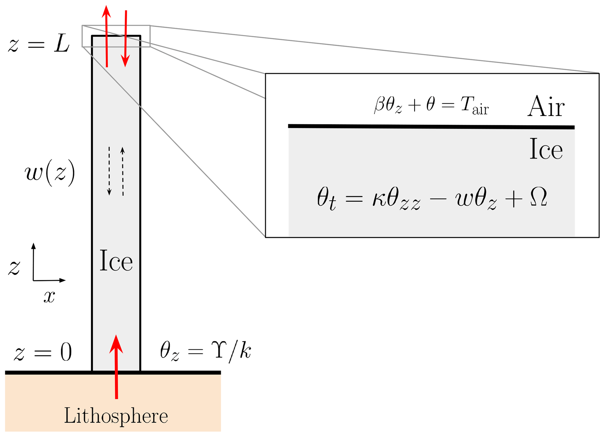
Figure 1 Schematic view of the 1D ice column with vertical advection w(z) and inhomogeneous term Ω (here, we independently consider both strain heating and depth-integrated horizontal advection). Temperature evolution is dictated by the heat equation and an appropriate set of initial and boundary conditions. Subscripts denote partial differentiation. At the top, both the ice temperature and the vertical gradient can vary in time, thus allowing for non-equilibrium thermal states across the ice–air interface. At the base, the vertical gradient is fixed at the value given by the combined contribution of geothermal heat flow and potential basal frictional heat, ${\mathit{\theta }}_z=-\mathrm{{\rm Y}}/k$. Note that our formulation is 1D, so the x axis is solely introduced for visualization.

In the simplest physical scenario, the ice surface temperature is set to the air temperature value $\mathit{\theta }(L,t)=T_{\mathrm{air}}$. However, surface temperatures are in fact the result of the energy balance between the ice and the atmosphere. To address this limitation, we refine the surface boundary condition by allowing for a potential deviation from the air temperature, accounting for the thermal insulating effect in the uppermost region of the ice column. This insulation effect is a direct consequence of the reduction in ice density towards the surface (e.g. Stevens et al., 2020) and, as a result, the reduced ice thermal conductivity (Sturm et al., 2002; Calonne et al., 2011, 2019). This surface energy balance falls within the so-called linear heat transfer boundary conditions or Newton's law of cooling (Carslaw and Jaeger, 1988, Chap. 1.9). Briefly, Newton's law of cooling states that the heat flux across the interface is proportional to the temperature difference between the surface and the surrounding medium. It is applicable to a large variety of conditions such as a body cooling by forced convection (i.e. a fluid forced rapidly past the surface of a solid) or a thin surface layer of a poor conductor (such as a low-density firn or snow layer above the glacial ice). Moreover, Newton's law of cooling captures the two simpler boundary conditions as limit cases: (1) prescribed surface temperature and (2) no heat flux across an interface.

This refinement enables a more accurate representation of the surface heat transfer dynamics and contributes to a comprehensive understanding of the energy balance within the ice column. In this description, both the surface ice temperature θ(L,t) and its vertical gradient θ_z(L,t) can vary in time:

$$\begin{array}{}\text{(1)}& \mathit{\beta }{\mathit{\theta }}_z+\mathit{\theta }=T_{\mathrm{air}},z=L,t>\mathrm{0},\end{array}$$

where italic subscripts denote partial differentiation and β is a parameter with length dimensions that modulates the permissible deviation between ice and air temperatures, often referred to as the surface thermal resistance (per unit area). We physically interpret β as the thermal insulation of the ice–air interface. In other words, β is a length scale over which the ice column feels the air temperature. A zero value corresponds to an ideal conductor $\mathit{\theta }(L,t)=T_{\mathrm{air}}$, whereas β→∞ represents a perfect thermal insulator characterized by a null heat exchange across the interface. In the limit case β=0, the ice–air interface is always at thermal equilibrium (i.e. θ=T_air). For β≠0, we allow for a heat exchange across the ice surface driven by the temperature difference between the two media. The thermal equilibrium is only reached if the ice surface and the atmosphere temperatures are identical. In such conditions, the heat flux across the interface is null and the vertical gradient at the top the ice column vanishes regardless of the value of β.

Considering diffusive heat transport, vertical advection and a potential heat source, the ice temperature θ(z,t) satisfies an initial value problem given by the heat equation:

$$\begin{array}{}\text{(2)}& \left\{\begin{array}{ll}{\mathit{\theta }}_t=\mathit{\kappa }{\mathit{\theta }}_{zz}-w{\mathit{\theta }}_z+\mathrm{\Omega },& z\in \mathcal{L},t>\mathrm{0},\\ \mathit{\theta }={\mathit{\theta }}_{\mathrm{0}}\left(z\right),& z\in \mathcal{L},t=\mathrm{0},\\ {\mathit{\theta }}_z=-\mathrm{{\rm Y}}/k,& z=\mathrm{0},t>\mathrm{0},\\ \mathit{\beta }{\mathit{\theta }}_z+\mathit{\theta }=T_{\mathrm{air}},& z=L,t>\mathrm{0},\end{array}\right.\end{array}$$

where the heat source Ω is an inhomogeneous term that captures strain heat and horizontal advection and $\mathrm{{\rm Y}}=G+Q$ is the combined contribution of geothermal heat flow G and potential basal frictional heat Q; k is the ice conductivity and κ is the ice diffusivity, both assumed to be constant. We further consider a z-dependent vertical velocity component given by w(z).

In order to solve this problem, we must first provide the particular form of the vertical velocity term. As in Clarke et al. (1977) and Zotikov (1986), we first assume a linear variation in w(z) with depth:

$$\begin{array}{}\text{(3)}& w\left(z\right)=w_{\mathrm{0}}{\displaystyle \frac{z}{L}},\end{array}$$

where w₀ is the vertical velocity at the ice surface z=L.

Standard values for w₀ usually read from −0.1 to −0.3 m yr⁻¹ (Glovinetto and Zwally, 2000; Spikes et al., 2004). Positive values of w₀ imply an upward movement of ice and are physically plausible, though quite rare. Dahl-Jensen (1989) calculated steady temperature distributions (their Fig. 5) and found that profiles near the terminus position resemble those predicted for an ablation zone (w₀>0). Solutions herein presented are applicable to both positive and negative values of w₀, though we will focus on the downward movement of ice (i.e. w₀<0). The linear dependency is widely used in the literature (e.g. Joughin et al., 2002, 2004; Suckale et al., 2014). Nonetheless, we will also explore a more general power-law relationship that better describes vertical velocities modelled by Glen's flow law (see Appendix C).

The inhomogeneous term Ω can encompass a number of heat sources and sinks. Here we focus on strain heating 𝒮 and horizontal advection ℋ, so $\mathrm{\Omega }=\mathcal{S}+\mathcal{H}$. In general, the strain heating term can be expressed as $\mathcal{S}={\mathit{\sigma }}_{ij}{\dot{\mathit{ϵ}}}_{ij}$, where σ_ij is the Cauchy stress tensor and ${\dot{\mathit{ϵ}}}_{ij}$ is the strain rate tensor (expressed in index notation). Upon application of Glen's law, the rate of strain heating is solely a function of the second invariant of the strain rate tensor:

$$\begin{array}{}\text{(4)}& \mathcal{S}={\mathit{\sigma }}_{ij}{\dot{\mathit{ϵ}}}_{ij}=\mathrm{2}{A}^{-\mathrm{1}/n}{\dot{{\mathit{ϵ}}_e}}^{(n+\mathrm{1})/n},\end{array}$$

where $\dot{{\mathit{ϵ}}_e}={\left({\dot{\mathit{ϵ}}}_{ij}{\dot{\mathit{ϵ}}}_{ij}/\mathrm{2}\right)}^{\mathrm{1}/\mathrm{2}}$ is the second invariant of the strain rate tensor and summation is implied over repeated indexes (Einstein notation). This formulation does not impose any conditions on the strain rate regime (i.e.  the dominant components) and only assumes $\dot{\mathit{ϵ}}$ to be constant in depth. This requirement ensures the analytical tractability of the solution while including a potential strain contribution throughout the ice column.

The horizontal advection term ℋ can imply a heat source or a sink, depending on the sign of the horizontal temperature gradient along a particular direction. We herein consider such a contribution by defining a depth-averaged lateral advection term (Meyer and Minchew, 2018):

$$\begin{array}{}\text{(5)}& \mathcal{H}={\displaystyle \frac{\mathrm{1}}{L}}\underset{\mathrm{0}}{\overset{L}{\int }}\left(\mathit{u}\cdot \widehat{\mathit{n}}\right){\mathit{\theta }}_{\widehat{\mathit{n}}}\mathrm{d}z,\end{array}$$

where u is the horizontal velocity vector, $\widehat{\mathit{n}}$ is the normal vector along an arbitrary direction contained in the horizontal plane, and ${\mathit{\theta }}_{\widehat{\mathit{n}}}=\partial \mathit{\theta }/\partial \widehat{\mathit{n}}$ denotes the directional derivative along $\widehat{\mathit{n}}$.

These assumptions allow us to include a potential strain heating source 𝒮 and a horizontal advection of heat term ℋ while keeping the analytical tractability of Eq. (2). The limitations of these simplifications are discussed in Sect. 7.

3 Analytical solution

We next outline our analytical approach. We first non-dimensionalize our problem and exploit the linearity of the differential operator by further decomposing the solution as a sum of stationary and transient components to deal with the inhomogeneity. Lastly, we apply a separation of variables to obtain a solution of the time-dependent problem and impose the corresponding initial and boundary conditions. Derivation details are elaborated in Appendix A.

It is natural to non-dimensionalize our problem by defining the following variables,

$$\begin{array}{}\text{(6)}& \begin{array}{rl}& \mathit{\xi }={\displaystyle \frac{z}{L}},\mathit{\tau }={\displaystyle \frac{\mathit{\kappa }}{L^{\mathrm{2}}}}t,\mathit{\theta }={\displaystyle \frac{T}{T_{\mathrm{air}}}},\stackrel{\mathrm{̃}}{w}={\displaystyle \frac{L}{\mathit{\kappa }}}w,\\ & \stackrel{\mathrm{̃}}{\mathit{\beta }}={\displaystyle \frac{\mathit{\beta }}{L}},\stackrel{\mathrm{̃}}{\mathrm{\Omega }}={\displaystyle \frac{L^{\mathrm{2}}}{\mathit{\kappa }{T}_{\mathrm{air}}}}\mathrm{\Omega },\end{array}\end{array}$$

over the domain $\stackrel{\mathrm{̃}}{\mathcal{L}}=[\mathrm{0},\mathrm{1}]$. Tildes are hereinafter dropped to lighten the notation.

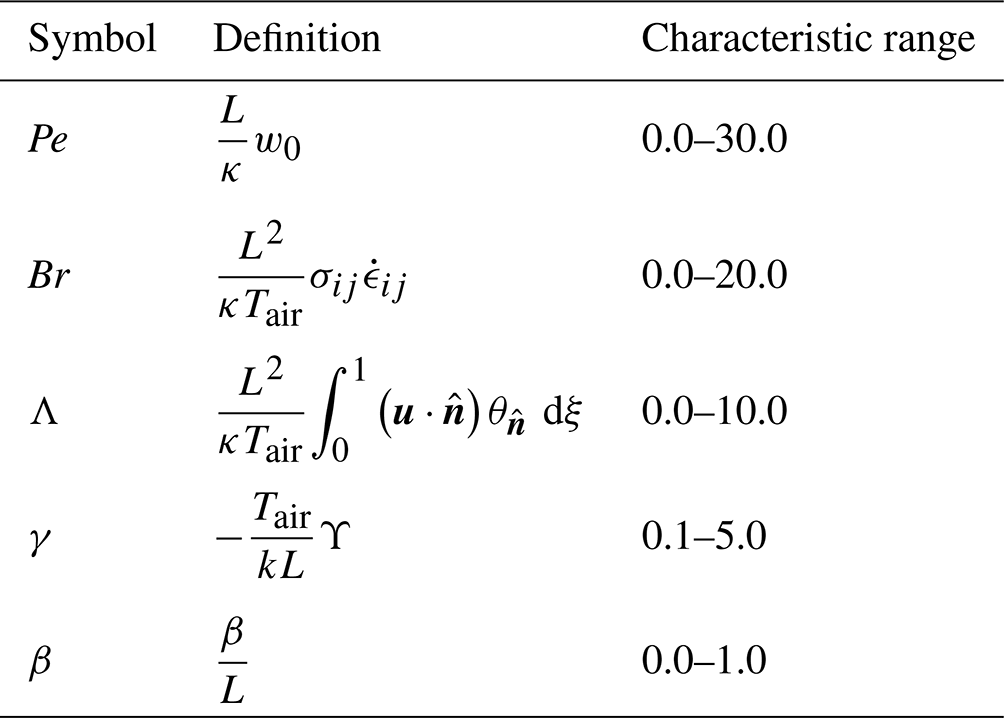
Table 1 Non-dimensional definitions and characteristic ranges. Summation is implied over repeated indices. Pe and Br are the Péclet and Brinkman numbers, respectively. Λ is the normalized horizontal advection, β is the surface insulation parameter, and γ is the dimensionless combined contribution of geothermal heat flow and basal frictional heat. Physical magnitudes employed to obtain these ranges are given in Table 2.

Hence, we can express our Eq. (2) as

$$\begin{array}{}\text{(7)}& \left\{\begin{array}{ll}{\mathit{\theta }}_{\mathit{\tau }}={\mathit{\theta }}_{\mathit{\xi }\mathit{\xi }}-\mathit{Pe}\mathit{\xi }{\mathit{\theta }}_{\mathit{\xi }}+\mathrm{\Omega },& \mathit{\xi }\in \mathcal{L},\mathit{\tau }>\mathrm{0},\\ \mathit{\theta }={\mathit{\theta }}_{\mathrm{0}}\left(\mathit{\xi }\right),& \mathit{\xi }\in \mathcal{L},\mathit{\tau }=\mathrm{0},\\ {\mathit{\theta }}_{\mathit{\xi }}=\mathit{\gamma },& \mathit{\xi }=\mathrm{0},\mathit{\tau }>\mathrm{0},\\ \mathit{\beta }{\mathit{\theta }}_{\mathit{\xi }}+\mathit{\theta }=\mathrm{1},& \mathit{\xi }=\mathrm{1},\mathit{\tau }>\mathrm{0},\end{array}\right.\end{array}$$

where $\mathit{\gamma }=-T_{\mathrm{air}}\mathrm{{\rm Y}}/\left(kL\right)$, w=Pe ξ and θ₀(ξ) are the non-dimensional geothermal heat flow, vertical velocity and initial profile, respectively. The vertical velocity is thereby conveniently expressed in terms of the Péclet number $\mathit{Pe}=w_{\mathrm{0}}L/\mathit{\kappa }$ (i.e. the ratio of advective to diffusive heat transport). The non-dimensional strain heating source term 𝒮 can be identified with the Brinkman number Br, which represents the ratio of deformation heating to thermal conduction (see Table 1). The non-dimensional number γ is the combined contribution of geothermal heat flow and potential basal frictional heat, normalized by the vertical temperature gradient that would exist for a column thickness L and temperature T_air. It provides the relative strength of the basal inflow of heat compared to the ice-column extent and the air temperature.

The dimensionless problem clearly shows that five numbers completely determine the shape of the stationary solution: γ, β, Pe, Λ and Br. Their particular impact on the temperature distributions is discussed below.

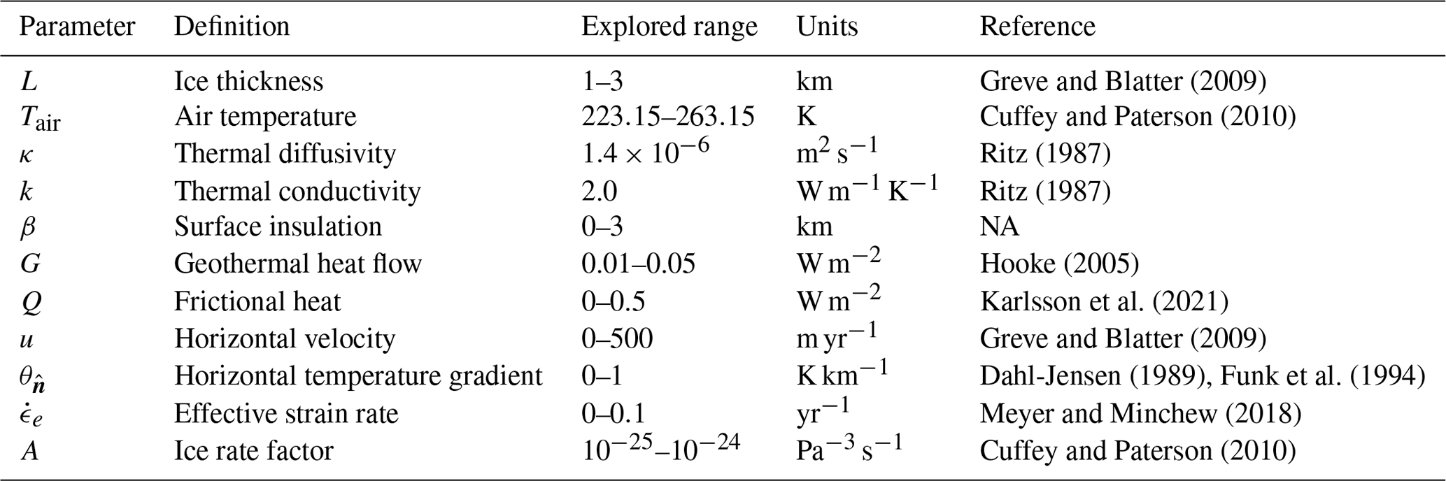
Greve and Blatter (2009)Cuffey and Paterson (2010)Ritz (1987)Ritz (1987)Hooke (2005)Karlsson et al. (2021)Greve and Blatter (2009)Dahl-Jensen (1989)Funk et al. (1994)Meyer and Minchew (2018)Cuffey and Paterson (2010)

Table 2 Physical parameter values employed to determine the non-dimensional range shown in Table 1.

NA: not available.

Given that Eq. (7) is inhomogeneous, we will decompose the solution as a sum of a transient μ(ξ,τ) and a stationary ϑ(ξ) components, so $\mathit{\theta }(\mathit{\xi },\mathit{\tau })=\mathit{\mu }(\mathit{\xi },\mathit{\tau })+\mathit{\vartheta }\left(\mathit{\xi }\right)$. As a result, the transient and stationary problems are subject to homogeneous and inhomogeneous boundary conditions, respectively:

$$\begin{array}{}\text{(8)}& \left\{\begin{array}{ll}{\mathit{\mu }}_{\mathit{\tau }}={\mathit{\mu }}_{\mathit{\xi }\mathit{\xi }}-w{\mathit{\mu }}_{\mathit{\xi }},& \mathit{\xi }\in \mathcal{L},\mathit{\tau }>\mathrm{0},\\ \mathit{\mu }={\mathit{\mu }}_{\mathrm{0}},& \mathit{\xi }\in \mathcal{L},\mathit{\tau }=\mathrm{0},\\ {\mathit{\mu }}_{\mathit{\xi }}=\mathrm{0},& \mathit{\xi }=\mathrm{0},\mathit{\tau }>\mathrm{0},\\ \mathit{\beta }{\mathit{\mu }}_{\mathit{\xi }}+\mathit{\mu }=\mathrm{0},& \mathit{\xi }=\mathrm{1},\mathit{\tau }>\mathrm{0},\end{array}\right.\end{array}$$

and

$$\begin{array}{}\text{(9)}& \left\{\begin{array}{ll}\mathrm{\Omega }={\mathit{\vartheta }}_{\mathit{\xi }\mathit{\xi }}-w{\mathit{\vartheta }}_{\mathit{\xi }},& \mathit{\xi }\in \mathcal{L},\\ {\mathit{\vartheta }}_{\mathit{\xi }}=\mathit{\gamma },& \mathit{\xi }=\mathrm{0},\\ \mathit{\beta }{\mathit{\vartheta }}_{\mathit{\xi }}+\mathit{\vartheta }=\mathrm{1},& \mathit{\xi }=\mathrm{1},\end{array}\right.\end{array}$$

where ${\mathit{\mu }}_{\mathrm{0}}={\mathit{\theta }}_{\mathrm{0}}\left(\mathit{\xi }\right)-\mathit{\vartheta }\left(\mathit{\xi }\right)$ is the initial profile of the transitory solution.

The solution to the stationary component (Eq. 9) already differs from previous analytical works like Robin (1955) and Lliboutry (1963). First, they considered a homogeneous version of the problem (i.e. Ω=0) so that potential strain heating or horizontal advective contributions are neglected. Moreover, they simplified the top boundary condition since they imposed a prescribed constant temperature value at ξ=1 (see also Clarke et al., 1977). However, our refinements still allow for analytical tractability, and thus the stationary solution is (see Appendix B for derivation details)

$$\begin{array}{}\text{(10)}& \mathit{\vartheta }\left(\mathit{\xi }\right)=\mathrm{\Omega }{\displaystyle \frac{{\mathit{\xi }}^{\mathrm{2}}}{\mathrm{2}}}{}_{\mathrm{2}}{F}_{\mathrm{2}}\left(\mathrm{1},\mathrm{1};{\displaystyle \frac{\mathrm{3}}{\mathrm{2}}},\mathrm{2};-\mathit{\zeta }\right)+A\mathrm{erf}\left[a\mathit{\xi }\right]+B,\end{array}$$

where ${}_{\mathrm{2}}{F}_{\mathrm{2}}(a_{\mathrm{1}},a_{\mathrm{2}};b_{\mathrm{1}},b_{\mathrm{2}},x)$ is the generalized hypergeometric function, ζ=(aξ)², $a={\left(w_{\mathrm{0}}/\mathrm{2}\right)}^{\mathrm{1}/\mathrm{2}}$, $A=-\mathit{\gamma }{\left(\mathit{\pi }/\left(\mathrm{4}a\right)\right)}^{\mathrm{1}/\mathrm{2}}$ and $B=\mathrm{1}-A\left(\mathrm{2}a{\mathit{\pi }}^{-\mathrm{1}}\mathit{\beta }{e}^{-a^{\mathrm{2}}}+\mathrm{erf}\left[a\right]\right)$. Note that if the inhomogeneous term is zero (i.e. Ω=0), the stationary temperature profile reduces to the well-known error function previously obtained by Robin (1955) and Lliboutry (1963). Even so, the temperature distribution would still differ as the boundary condition considered herein reflects a potential surface thermal insulation unlike prior studies.

We now take a step further and allow for time evolution by solving Eq. (8) and building our solution as the sum of both contributions. Namely, the general solution of the transient problem μ(ξ,τ) is (see Appendix A for derivation details)

$$\begin{array}{}\text{(11)}& \mathit{\mu }(\mathit{\xi },\mathit{\tau })=\sum _{n=\mathrm{0}}^{\mathrm{\infty }}\left[A_n\mathrm{\Phi }\left({\mathit{\alpha }}_n;\mathit{\delta };\mathit{\zeta }\right)+B_n\mathrm{\Psi }({\mathit{\alpha }}_n;\mathit{\delta };\mathit{\zeta })\right]e^{-{\mathit{\lambda }}_n\mathit{\tau }},\end{array}$$

where $\mathrm{\Phi }\left(\mathit{\alpha };\mathit{\delta };\mathit{\zeta }\right)$ and $\mathrm{\Psi }\left(\mathit{\alpha };\mathit{\delta };\mathit{\zeta }\right)$ are the Kummer (Kummer, 1836) and Tricomi confluent hypergeometric functions, respectively (also known as confluent hypergeometric functions of the first and second kind). ${\mathit{\alpha }}_n=-{\mathit{\lambda }}_n/\left(\mathrm{2}{w}_{\mathrm{0}}\right)$ and $\mathit{\delta }=\mathrm{1}/\mathrm{2}$. As the solution must be bounded at the origin, we set B_n=0.

The full solution $\mathit{\theta }(\mathit{\xi },\mathit{\tau })=\mathit{\vartheta }\left(\mathit{\xi }\right)+\mathit{\mu }(\mathit{\xi },\mathit{\tau })$ thus reads

$$\begin{array}{}\text{(12)}& \begin{array}{rl}\mathit{\theta }(\mathit{\xi },\mathit{\tau })& =\mathrm{\Omega }{\displaystyle \frac{{\mathit{\xi }}^{\mathrm{2}}}{\mathrm{2}}}{}_{\mathrm{2}}{F}_{\mathrm{2}}\left(\mathrm{1},\mathrm{1};{\displaystyle \frac{\mathrm{3}}{\mathrm{2}}},\mathrm{2};-\mathit{\zeta }\right)\\ & +A\mathrm{erf}\left[a\mathit{\xi }\right]+B+\sum _{n=\mathrm{0}}^{\mathrm{\infty }}{A}_n\mathrm{\Phi }\left({\mathit{\alpha }}_n;\mathit{\delta };\mathit{\zeta }\right)e^{-{\mathit{\lambda }}_n\mathit{\tau }},\end{array}\end{array}$$

where the coefficients A_n are obtained from the initial temperature profile (Eq. A13 in Appendix A).

4 Stationary solutions

Before displaying the results of the full time-dependent problem, it is worth describing the temperature solutions at equilibrium.

Figure 2 shows our steady-state solutions as vertical profiles for a subset of the permutations of the non-dimensional numbers Pe, Br, γ, Λ and β. It is illustrative to compare the shape of our temperature solutions with Clarke et al. (1977) (their Fig. 1). We must stress that a one-to-one comparison is not readily possible since they imposed a simpler top boundary condition in which the ice surface temperature is fixed at a given value, though the exact same solutions can be simply obtained by setting β=0 in our case (see Eq. 1).

The non-dimensionalization of our analytical model provides simplicity and further reduces the parameter dimensionality of the solutions to solely five numbers, each corresponding to one column in Fig. 2. The Péclet number produces significant changes in the equilibrium solutions, as colder ice is advected from the uppermost part of the column, consequently cooling down the profile with increasing Pe values (Fig. 2a), in contrast to the well-known linear profile resulting for the purely diffusive case (i.e. Pe→0). The combined contribution of geothermal heat flow and friction heat dissipation γ also yields large temperature amplitudes within the explored range. Nevertheless, the impact is clearly limited to the lower half of the column, thus leaving the upper regions nearly unperturbed, as shown in Fig. 2c. Likewise, for the surface insulation parameter β in the presence of downwards advection (Pe=7), the entire temperature profile is left unchanged despite varying values of β (Fig. 2b). This can be understood as the heat exchange at the ice–air interface not being relevant for the strong downward transport of colder ice, which is a far more effective heat transport compared to dissipation. Unlike γ, the strain heat dissipation Br influences the upper region of the ice temperature as its contribution is distributed throughout the column (Fig. 2d) rather than being a basal heat source. Even so, the impact is most notable near the base given that the temperature therein can freely evolve so long as the geothermal heat flow condition is met (Eq. 2). Similarly, the vertically averaged lateral heat advection Λ also affects upper regions of the column (Fig. 2e). Here we have chosen positive Λ values, implying advection of colder ice. As a result, for sufficiently large values of Λ, the temperature within the column can be lower than at the surface, reaching a local minimum therein and gradually increasing as the base is approached. For negative values of Λ, we would find temperature profiles like those obtained in Fig. 2d.

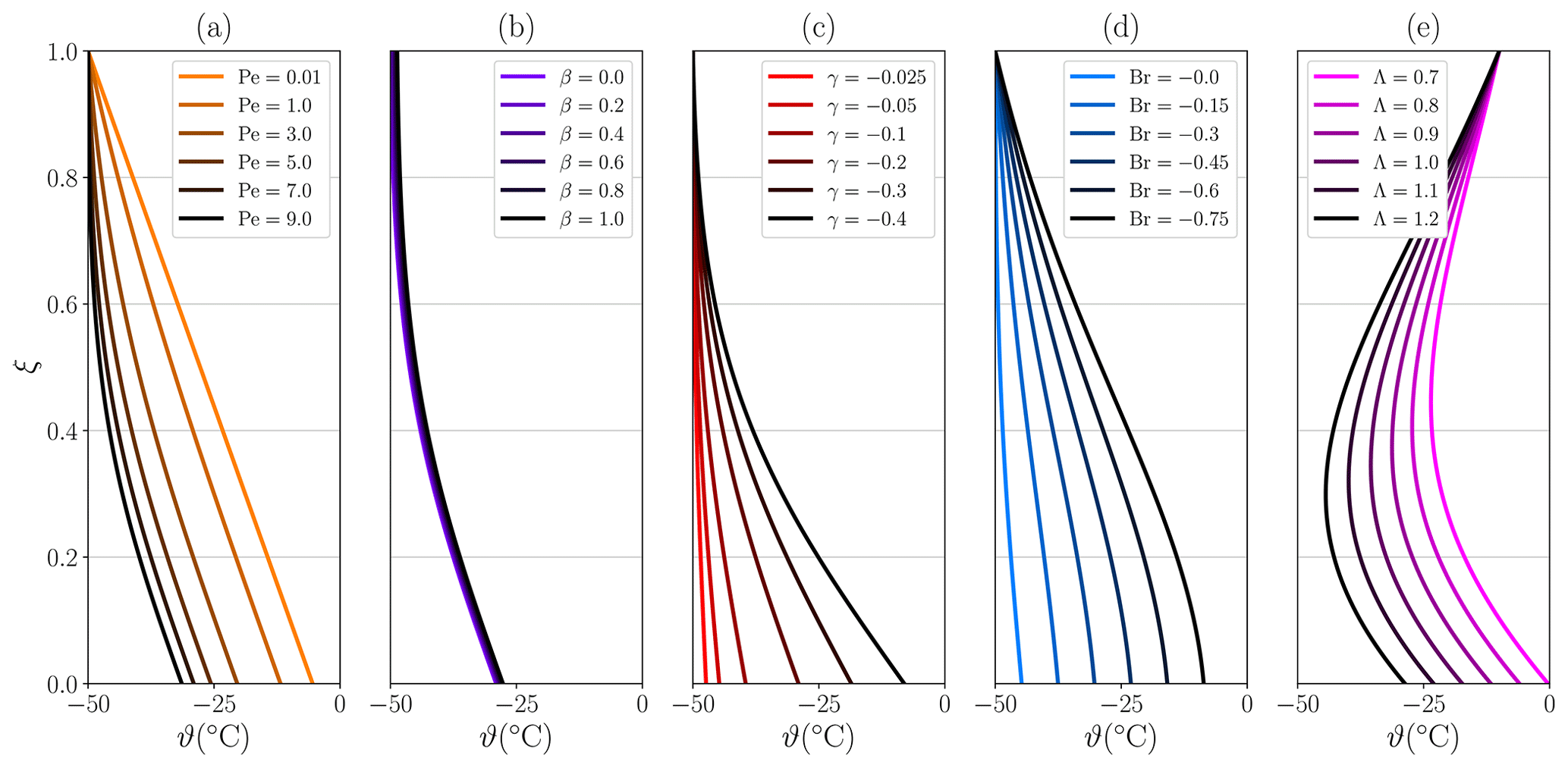
Figure 2 Stationary temperature profiles ϑ(ξ). (a–e) Solutions are fully determined by five non-dimensional numbers: Pe, β, γ, Br and Λ, corresponding to each panel, respectively. Default values are Pe=5, β=0, $\mathit{\gamma }=-\mathrm{0.2}$, Br=0 and Λ=0, except for panel (e), where $\mathit{\gamma }=-\mathrm{0.4}$.

5 Full solutions

We now present the results of the full problem presented in Eq. (2) by including the time-dependent solution. This transient nature depends on the initial state of the system, although it exponentially converges to the steady state as the transient component vanishes under the assumption of constant boundary conditions. We further overcome the arbitrariness of the initial temperature profile by directly calculating the eigenvalues of the problem and their corresponding decay times as an estimation of the timescale of our system in different physical scenarios.

To illustrate the full solutions, we show the explicit time evolution from an initial profile as it approaches the corresponding stationary solution (Fig. 3). In this instance, we employ constant initial temperature profiles for simplicity, θ₀(ξ)=0.5 and θ₀(ξ)=2.5 in Fig. 3a and b, respectively. With these particular choices, we ensure that the initial temperature profile is below and above the stationary solution for two strong advective scenarios: vertical and lateral. Figure 3a shows how temperature both at the ice surface and most notably at the base starts to increase for τ>0, while at the central region of the column it remains constant until heat propagates along the column. It is worth noting how the surface temperature gradually relaxes to the equilibrium profile, since instead of imposing the air temperature, a more realistic heat exchange at the ice–air interface is considered via β=0.5. In contrast, Fig. 3b shows an instantaneous change at the surface by an oversimplified top boundary condition if β=0 (i.e. a perfectly conductive ice–air interface). As a result, the cold air temperature rapidly propagates into the uppermost region of the ice column rapidly, whereas the geothermal heat flow contribution requires a longer time to propagate from the base. In contrast, the lower part of the domain increases its temperature notwithstanding the sudden decrease in the upper region. As the column evolves in time, the rate of change gradually diminishes, and it approaches zero as the transient solution asymptotically reaches the temperature profile given by the stationary temperature profile $\mathit{\vartheta }\left(\mathit{\xi }\right)={lim}_{\mathit{\tau }\to \mathrm{\infty }}\mathit{\theta }(\mathit{\xi },\mathit{\tau })$.

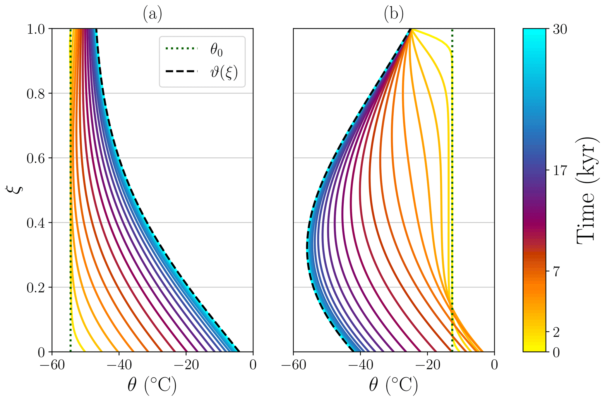
Figure 3 Time-dependent solution θ(ξ,t) given an initial temperature profile θ₀(ξ) (vertical dotted line). Dimensionless values: (a) β=0.5, Λ=0 and (b) β=0.0, Λ=1.0. Default values: Pe=5.0, $\mathit{\gamma }=-\mathrm{0.35}$, Br=0. Dashed black lines represent the stationary solution ϑ(ξ). To ease visualization, the time variable is quadratically spaced as indicated in the colour bar.

To examine the transient nature of the solutions closely, we present the temperature evolution of a given initial profile for a certain range of the non-dimensional parameters (Fig. 4). This gives us information about the time-dependent effects of each parameter, unlike Fig. 2, which is restricted to equilibrium states. Additionally, the continuous representation (i.e. colour bar in Fig. 4), as opposed to the discrete number of vertical profiles in Fig. 3, facilitates comparison among particular parameter choices.

The particular parameter values were selected so that we could obtain four physically distinct scenarios: (a) high geothermal heat flow under a large advection regime, (b) high strain heat dissipation in a low-vertical-advection regime, (c) strong lateral advection of colder ice under surface insulating conditions and (d) weak geothermal heat flow under a low-vertical-advection regime. This setup allows us to separately determine the role played by each mechanism during the transient regime of the solution.

Figure 4a shows that the thermal equilibration begins by an increase in the basal temperature that gradually propagates upwards until it is balanced by the downward advection of ice from the colder surface. A similar transient behaviour is found if strain heat dissipation is additionally considered (Fig. 4b). Even though the geothermal heat flow is significantly smaller in this scenario, the heat travels further upwards as a result of a low-vertical-advection regime (Pe=2) combined with a source of strain heat throughout the column (Br=6). If we instead consider a scenario where heat is removed by lateral advection of colder ice Λ=6 (Fig. 4c), we note two different timescales: the geothermal heat flow first warms the ice base, and then the lateral removal of heat takes over with a consequent reduction in temperature in the entire column. Lastly, a low basal inflow of heat combined with a weak vertical advective regime (Fig. 4d) yields the smallest temperature gradients within the column.

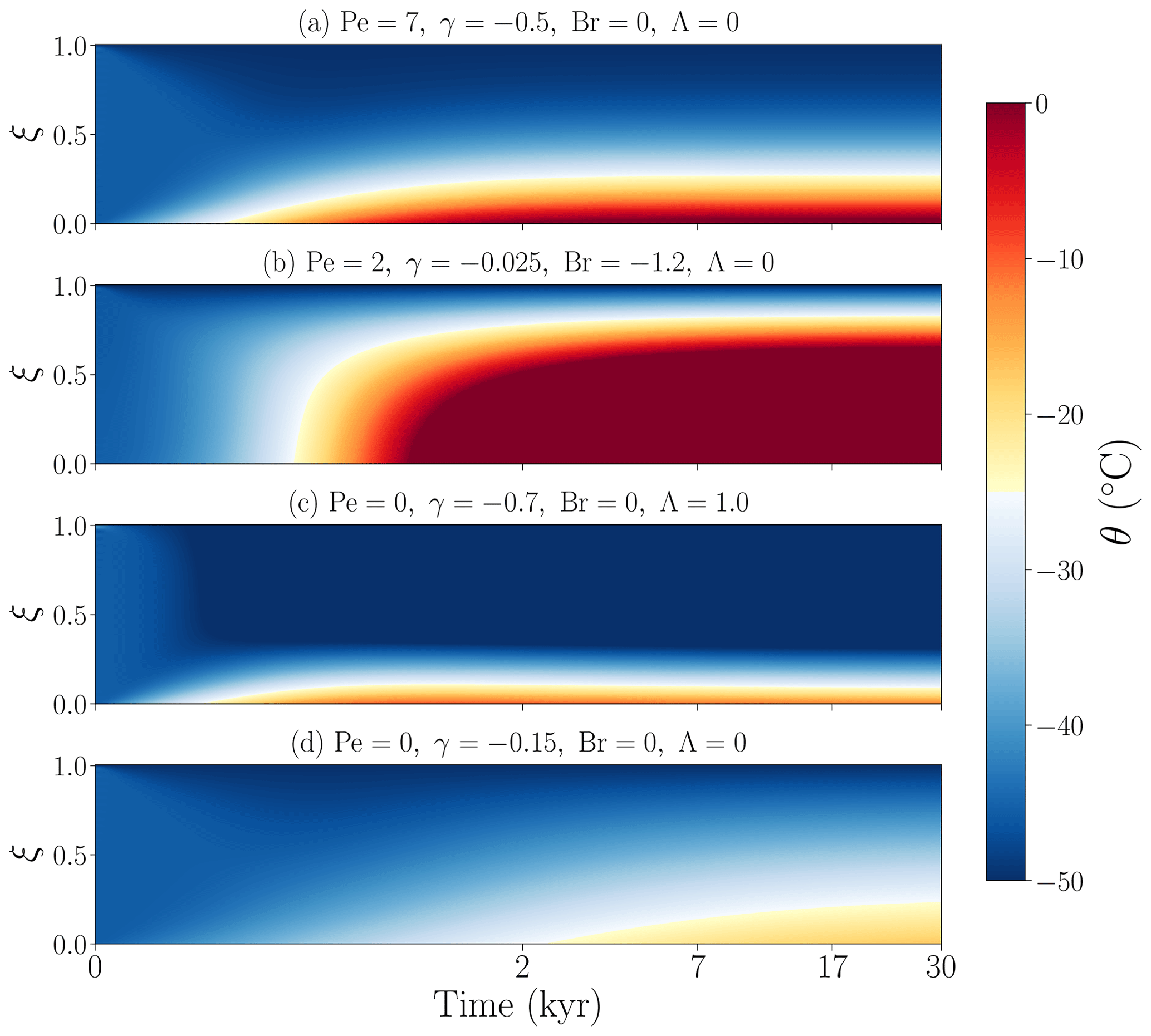
Figure 4 Time-dependent solution θ(ξ,τ) given an initial temperature profile. For simplicity, here the initial temperature profile is ${\mathit{\theta }}_{\mathrm{0}}\left(\mathit{\xi }\right)=-\mathrm{40}$ °C at all depths and in all cases.

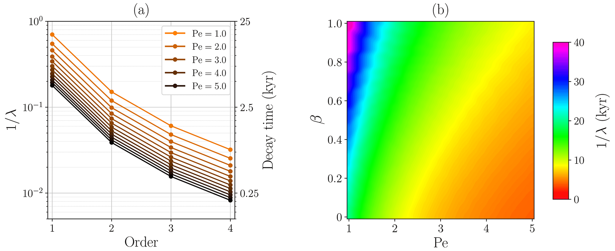
We can also predict the behaviour of the transitory component directly from the eigenvalues of the problem. By calculating the inverse of the eigenvalues ${\mathit{\lambda }}_n^{-\mathrm{1}}$, we obtain a magnitude that can be expressed with time dimensions and represents the decay time of each Fourier mode (Fig. 5a). Physically, this is the time required for the transient component to be reduced a factor e⁻¹ at any point, and it further allows us to estimate the equilibration time from an arbitrary initial state. As we would expect, higher-order modes have a shorter lifetime. Notably, the eigenvalue equation solely depends on Pe and the surface insulation parameter β (Eq. A8, Appendix A). This implies that the time to reach equilibrium exclusively depends on these two numbers. The remaining dimensionless parameter values yield the exact same equilibration time despite playing a role in the particular form of the solution. In other words, the five dimensionless numbers shape the temperature profile, but only the vertical advection and the surface insulation parameter influence the exponential decay of the transitory component and, therefore, the timescale to reach equilibrium from an arbitrary initial state (Fig. 5b). Particularly, scenarios with a high-advective regime yield shorter equilibration times (∼2–10 kyr; Fig. 5b), unlike highly insulating scenarios at the surface, characterized by long decay times (∼25–40 kyr).

Figure 5 Decay time and corresponding eigenvalues. (a) First four eigenvalues for the set of β values shown in Fig. 2b. (b) Decay time (kyr) of the first eigenvalue as a function of Pe and β.

6 Benchmarks for numerical solvers

The analytical solutions obtained herein are valuable tools for testing numerical solvers. We thus propose a suite of benchmark experiments with gradually increasing complexity to test the representation of each physical process involved in ice temperature evolution (see Table 3).

Table 3 Benchmark experiments for numerical solvers and main physical processes considered for heat propagation. The experiments are named in increasing complexity order.

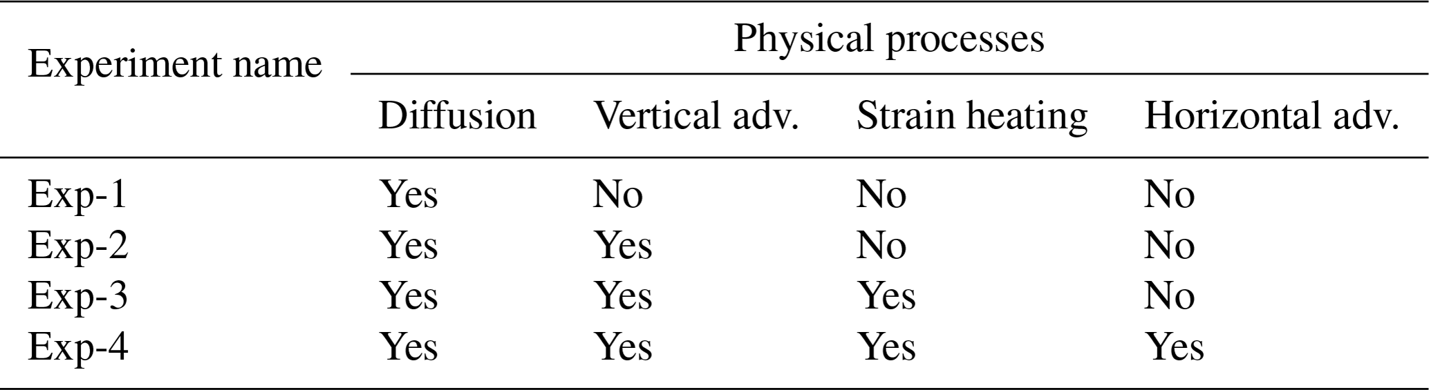
First, we simply consider the well-known purely diffusive case (Exp-1). Then, vertical advection is additionally included (Exp-2). Lastly, strain heating (Exp-3) and the vertically averaged horizontal advection (Exp-4) are considered. Given the analytical nature of our solutions, spatial and temporal resolutions can be set arbitrarily high as there are neither convergence nor stability constraints. This allows for a comparison against spatial and temporal resolutions found in numerical solvers. We must stress that the initial temperature profile and all other parameters can be set by the user to test the solution for any desired scenario. We also note that these are simply proposed benchmarks, but the solutions developed here can be used for any type of benchmark test that is desired and fits the limitations of the equations.

We develop a numerical model for testing by performing a finite-difference discretization of Eq. (7) and the basal boundary condition over a sigma coordinate system, where grid points are unevenly spaced. This nonuniform grid can follow either a quadratic or an exponential relation, set by the user. This yields higher resolutions near the base for a fixed number of points, thus minimizing the computational costs. Several discretization schemes are employed with varying orders of convergence, summarized in Table 4. Numerical solutions are then compared at equilibrium with their analytical counterpart (Fig. 6).

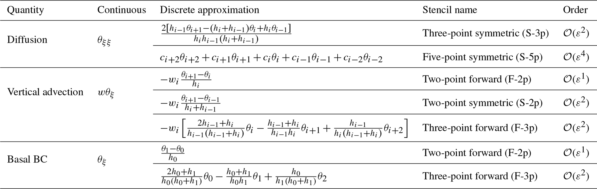
Table 4 Finite-difference approximations employed in the numerical study (Fig. 6) for unevenly spaced grids ζ_i, as detailed in Appendix D. Distance between two adjacent points is defined as $h_i={\mathit{\zeta }}_{i+\mathrm{1}}-{\mathit{\zeta }}_i$. Note that vertical velocities are negative (downwards movement of ice) and the advection stencils are consequently adjusted. Discretization coefficients for the S-5p scheme are given in Appendix D. BC signifies the boundary condition.

As could be expected, Fig. 6 illustrates that spatial discretization becomes a fundamental piece to obtain an accurate temperature solution, particularly at the base of the ice. The purely diffusive scenario (Exp-1; Fig. 6a) shows the smallest (negligible) errors for all discretization schemes given its mathematical simplicity. If vertical advection is further introduced (Exp-2; Fig. 6), the particular choice by which the temperature first derivative θ_ξ is discretized becomes important, as temperature gradients can be transported via non-zero vertical velocities. Forward stencils slightly overestimate (F-2p) and underestimate (F-3p) the solution as shown in Fig. 6b. In contrast, symmetric stencil S-2p provides a numerical solution significantly closer to the analytical profile, particularly near the base. The next benchmark experiment (Exp-3; Fig. 6c), where the inhomogeneous term captures a source of heat throughout the column due to strain deformation, presents a similar behaviour, where the F-3p stencil underestimates the solution. Again, the symmetric scheme outperforms the asymmetric ones. Lastly, the inhomogeneous term is introduced, physically capturing a vertically averaged source or sink of heat as a consequence of the advected ice in the horizontal dimension. We thus considered a negative contribution that physically describes a downstream advection of colder ice (Exp-4; Fig. 6d). Numerical solutions overestimate the analytical solution for the asymmetric discretization schemes (i.e. F-2p and F-3p), unlike the two-point symmetric scheme (S-2p). It is worth noting that the closest result to the analytical solution is obtained using S-2p for the advective term and F-3p for boundary condition discretization. In the remaining experiments, the particular scheme employed in the basal boundary condition does not modify the solution.

For all experiments tested, results are identical irrespective of the particular discretization of the diffusion term (Table 4), so both the three-point and the five-point symmetric stencils yield the same stationary temperature profiles. Overall, all finite-difference stencils herein presented successfully converge (Fig. 6e) for all benchmark experiments, yielding the smallest residual error for the purely diffusive scenario (Exp-1).

Additionally, we perform a resolution convergence test for the best discretization choice (Table 4): F-3p for the diffusive term, S-2p for vertical advection and F-3p for basal boundary condition. In order to quantify the residual error as a function of the spatial resolution for each benchmark experiment (Fig. 7), we compute the ℓ² norm of the difference between the numerical and the analytical solutions $\mathit{\epsilon }=\left|\right|{\mathit{\vartheta }}_{\mathrm{num}}-\mathit{\vartheta }|{|}_{{\mathrm{\ell }}^{\mathrm{2}}}$, defined as $\left|\right|\mathit{x}|{|}_{{\mathrm{\ell }}^{\mathrm{2}}}={\left({\sum }_i{x}_i^{\mathrm{2}}\right)}^{\mathrm{1}/\mathrm{2}}$. The larger deviations from the analytical solutions are found for the lower half of the ice column and are strongly dependent on the vertical resolution. Results show that a coarse resolution tends to overestimate the equilibrium temperature for all benchmark experiments. The residual error between the analytical and numerical solution exponentially decays, reaching values of $\mathit{\epsilon }<{\mathrm{10}}^{-\mathrm{2}}$ for n>15.

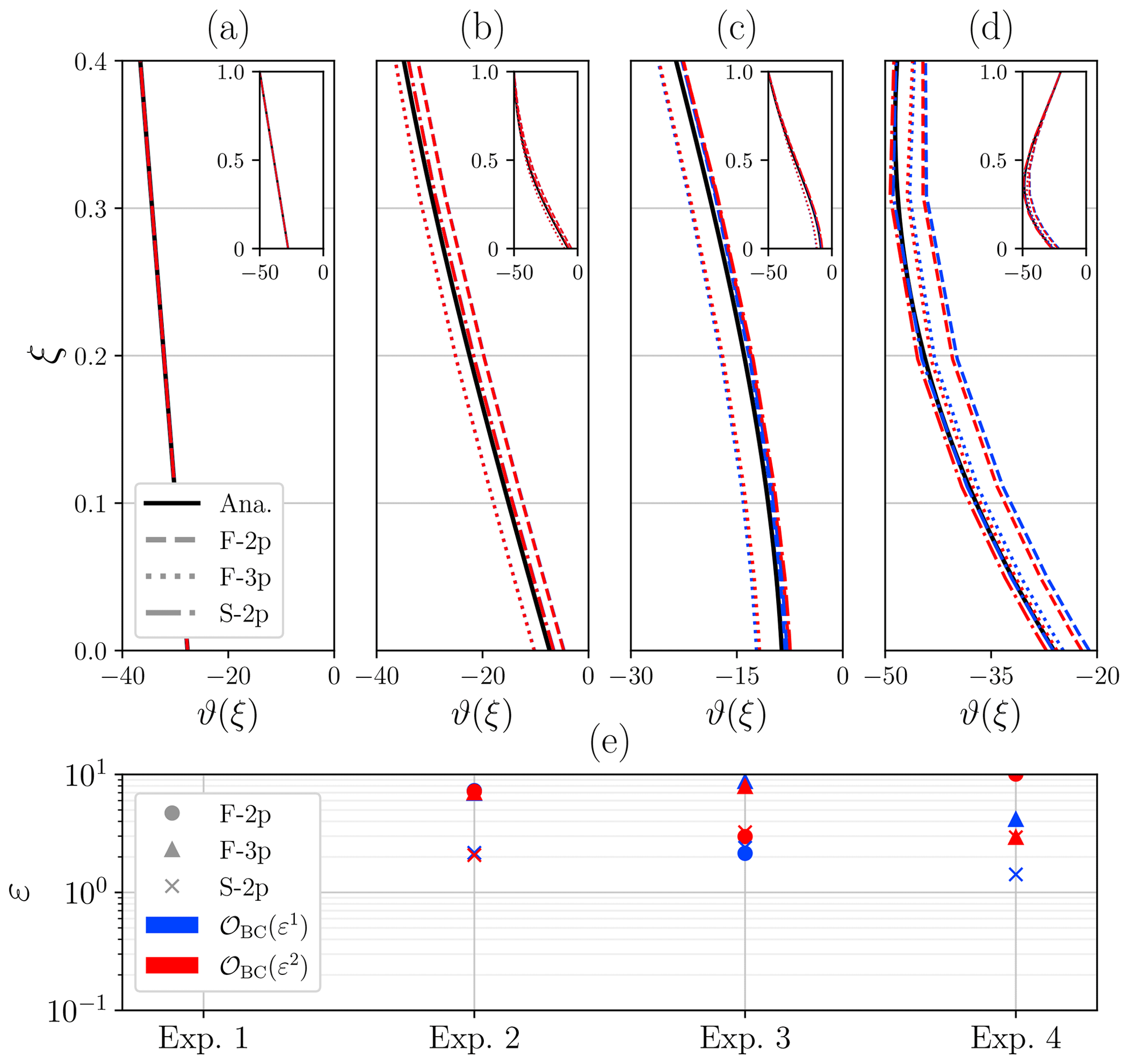
Figure 6 (a–d) Numerical steady-state solutions (red, blue) for all discretizations shown in Table 4 compared with the analytical solution (solid black). (e) Residual error defined as the difference between the numerical and the analytical solutions $\mathit{\epsilon }=\left|\right|{\mathit{\vartheta }}_{\mathrm{num}}-\mathit{\vartheta }|{|}_{{\mathrm{\ell }}^{\mathrm{2}}}$. Colour code represents the two asymmetric discretization schemes for the basal boundary condition: F-2p (blue) and F-3p (red). Marker and line styles denote the discretization stencil of the vertical advective term. The number of vertical points n=10 is fixed for all cases. Numerical solutions are identical upon spatial discretization of the diffusive term at orders 𝒪(ε²) and 𝒪(ε⁴) (see Table 4). The purely diffusive case (Exp. 1) yields negligible errors $\mathit{\epsilon }<{\mathrm{10}}^{-\mathrm{5}}$.

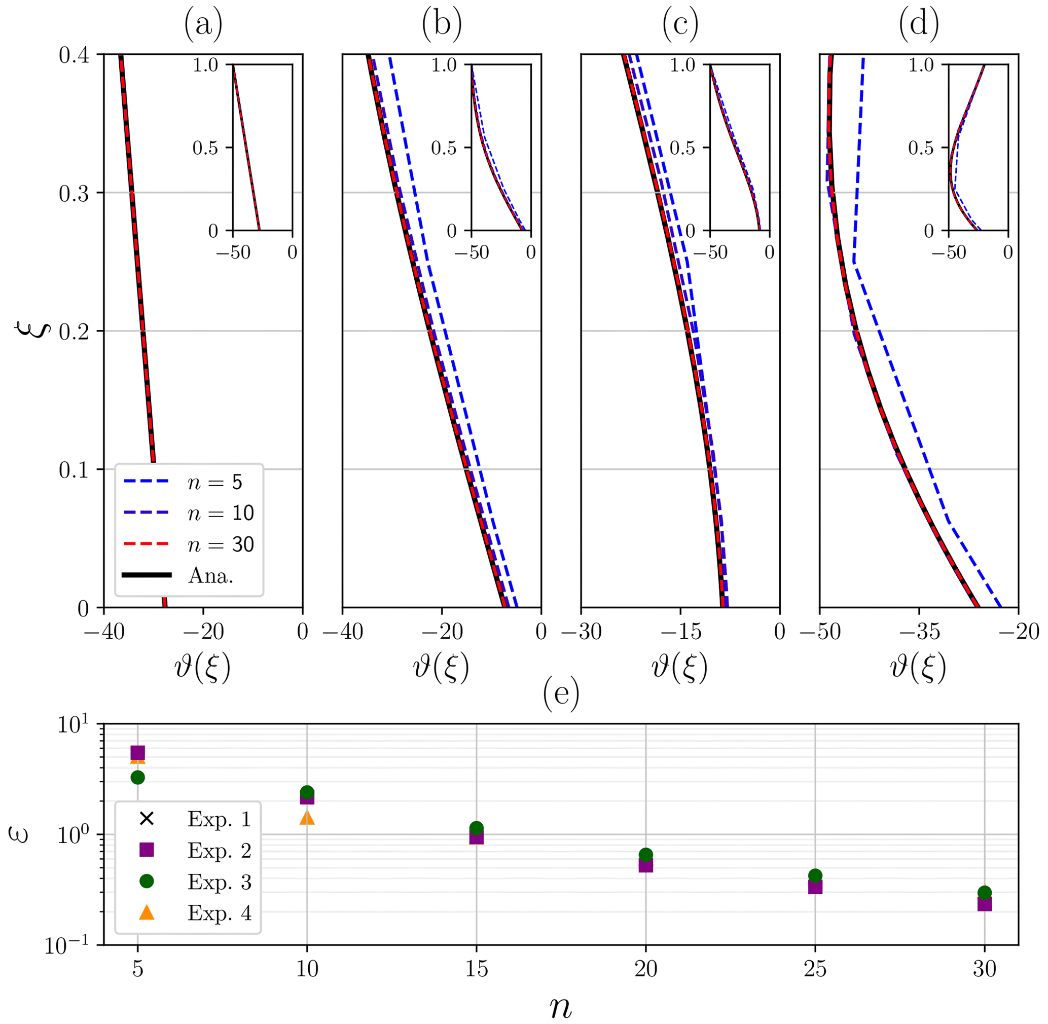
Figure 7 Convergence study of benchmark experiments. Steady-state analytical solutions shown with the solid black line. (a) Exp-1, (b) Exp-2, (c) Exp-3 and (d) Exp-4. (e) Residual error defined as the difference between the numerical and the analytical solutions $\mathit{\epsilon }=\left|\right|{\mathit{\vartheta }}_{\mathrm{num}}-\mathit{\vartheta }|{|}_{{\mathrm{\ell }}^{\mathrm{2}}}$. For all experiments, γ=2 and β=0.

7 Discussion

The adoption of dimensionless variables results in enhanced generality and mathematical convenience, albeit at the expense of veiling the practical significance to real glaciers and ice sheets. We have consequently tabulated data for characteristic values to ease interpretation (Table 1), thus showing that the explored range encompasses realistic values found in ice caps (Table 2).

We first start by comparing our results with a previously obtained solution for a simpler case (e.g. Clarke et al., 1977). We obtain identical results by setting the ice surface temperature to a fixed value given by the air temperature, i.e. imposing β=0 in Eq. (2) (Fig. 2c and f). Prominently, note that a non-zero β value is fundamental in the transitory regime (Fig. 11), though it leads to negligible changes at equilibrium (Fig. 2).

The transient behaviour of the solution is intricate given the freedom to choose an arbitrary initial state. This issue can be overcome by direct inspection of the eigenvalues of the problem. An estimation of the decay time of the analytical solution shows that the advection and the surface insulation are the only parameters that determine the timescale to reach thermal equilibrium. This approach has some limitations, some of which we now discuss. The decay time dependency is subjected to the mathematical form of our problem (Eq. 2). If an analytical solution could be obtained with an additional explicit horizontal advection term (rather than a vertically averaged contribution), then the eigenvalues, and consequently the decay times, would also depend on Λ. A second limitation concerns the boundary conditions. This solution required time-independent conditions, and therefore the decay time estimations do not hold if, for instance, the surface temperature changes over time. Even so, the approach developed here provides estimates of relaxation times under different physical conditions and gives an explicit expression for the time-dependent temperature profile from any arbitrary initial state.

The tractability of the analytical solution does not allow for further complexity, and hence additional numerical methods would be necessary if such a physical description is desired. Nonetheless, a constant horizontal advection term Λ was also introduced as part of the inhomogeneous term Ω, for which the sign of the horizontal temperature gradients must be chosen a priori. Even though horizontal variability in temperature distributions can vary greatly, we account for this effect by assuming a constant term (throughout the ice column) entering the heat equation, thus not reflecting much of the non-local features of the thermal structure of the ice sheets.

It must be stressed that our analytical solutions are not limited to regions with negligible horizontal velocities, since the true constraining quantity is the vertical gradient of the horizontal velocity u_z. Hence, rapidly sliding regions with a small vertical gradient of the horizontal velocity are also suitably described by our solutions, for which u_z≃0 implies that the temperature profile is merely transported along the flow direction while compressing the temperature gradient as the ice stream thins (Robel et al., 2013). One can argue that the additional source of heat due to frictional dissipation should be also considered therein. Nonetheless, in terms of the temperature distribution, this effect is equivalent to an increased geothermal heat flow, as it is purely restricted to the column base and therefore already encompassed in Eq. (7).

The strain rate regime poses further limitations on the applicability of the solution. Particularly for regions where vertical shear dominates and the strain heat dissipation is concentrated near the base, a vertically averaged contribution appears to be inaccurate. Nevertheless, as already noted by Rezvanbehbahani et al. (2019), this effect is instead well-captured by an increase in the inflow of heat from the base (i.e. equivalent to a larger geothermal or frictional heat term) under conditions where most of the vertical shear is concentrated in the basal layers (Fowler, 1992).

It is worth noting that phase changes are not considered herein, so temperature evolution is strictly confined to values below the pressure melting point. Unlike a numerical solver, where temperature is manually limited, these solutions must be taken with caution as we are describing a frozen ice column. Results are still compatible with a potential heat contribution due to basal frictional heat (Eq. 2), even though fast-sliding regions are often related to temperate basal conditions. Nevertheless, an additional heat contribution would imply an increased vertical temperature gradient even if the column base eventually reached the pressure-melting point.

Knowing that ice forms by snow densification through time (Stevens et al., 2020), we find layers of progressively increasing ice density descending from the surface. Likewise, snow thermal conductivity increases with density (e.g. Sturm et al., 1997, 2002; Calonne et al., 2011, 2019), resulting in a poorer heat conductor as the snow–air interface is approached. As already noted by Carslaw and Jaeger (1988), if the flux across a surface is proportional to the temperature difference between the surface and the surrounding medium, the appropriate boundary condition takes the form of Eq. (1) rather than the oversimplified version $\mathit{\theta }(L,t)=T_{\mathrm{air}}$. Here we explicitly describe the ice column with a constant thermal conductivity to keep analytical tractability, but we aim at describing the fact that the thermal conductivity of glacial ice k(ρ) is reduced towards the surface. Following Carslaw and Jaeger (1988), we apply a general Newton's law that also captures the traditional approach (i.e. imposing a particular ice surface temperature given by the air temperature) as a limit case if β→0.

Our suite of benchmark experiments allows us to test numerical solvers and assess reliability for different discretization schemes and resolutions. The basal boundary condition is sensitive to the particular discretization scheme, as the geothermal flux is the main source of heat in the ice column and is considered via a Neumann boundary condition. The simplest two-point stencil does not correctly represent the equilibrium temperatures, yielding larger deviations at the base (Fig. 6). Higher-order discretizations are necessary to obtain a more reliable temperature distribution. In our benchmark experiments, we find significant improvement between the 𝒪(ε¹) and 𝒪(ε²) schemes for the basal boundary condition (Fig. 6), particularly for scenarios with large strain heating values or strong horizontal heat advection. Results for the different vertical advection schemes show that forward stencils (both F-2p and F-3p) deviate further from the analytical solution when compared to a symmetric scheme. Despite the fact that symmetric advective schemes might show some instabilities, we have not found any numerical issues in the present study. In contrast, such schemes appear to outperform the asymmetric counterparts for all benchmark experiments.

Resolution plays a fundamental role in obtaining a reliable temperature profile. A sigma coordinate system with quadratic spacing accurately ($\mathit{\epsilon }<{\mathrm{10}}^{-\mathrm{2}}$) reproduces the analytical solution for n≥15 grid points and provided our best numerical scheme choice. Additional calculations performed for an exponential grid spacing (not shown) reveal consistent results with the quadratic dependency (Figs. 6 and 7). This shows the robustness of our numerical schemes, in which the symmetric advective stencil (S-2p) and the three-point basal boundary conditions (F-3p) again outperform the remaining choices.

8 Conclusions

We have determined the analytical solution to the 1D time-dependent advective–diffusive heat problem including additional terms due to strain rate deformation and depth-integrated horizontal advection. A Robin-type top boundary condition further considers potential non-equilibrium temperature states across the ice–air interface. The solution was expressed in terms of confluent hypergeometric functions following a separation of variables approach. Non-dimensionalization reduced the parameter space to five numbers that fully determine the shape of the solution at equilibrium. We further overcome the arbitrariness of the initial temperature profile by directly calculating the eigenvalues of the problem and their corresponding decay times as an estimation of the timescale of our system in different physical scenarios. The transient component exponentially converges to the stationary solution with a decay time that solely depends on vertical advection and surface insulation.

The sign of vertical advection is of utmost importance as it determines the direction along which temperature gradients are transported. We have focused in the present study on the downward advective scenario, given the implausibility of an upward advection of ice. At equilibrium, basal temperatures are particularly sensitive to four physical quantities: vertical advection, geothermal heat flow, strain heat and lateral advection. In contrast, the surface insulation yields negligible changes in the stationary solution. This is true even for highly insulating conditions at the ice surface, so long as colder ice is transported more efficiently than heat travels upwards due to diffusion.

The transient regime shows a strongly distinct behaviour. The arbitrariness of the initial state is overcome by a direct inspection of the eigenvalues of the problem. We then obtain a magnitude that represents the decay time of each Fourier mode that provides information about the equilibration time of the system. We find that the decay time of the transient component solely depends on two magnitudes: advection (Pe) and surface insulation (β). The remaining dimensionless parameters shape the temperature solution, though they have no influence on the timescale to reach thermal equilibrium. Strong advective regimes (Pe∼5) yield ∼2–10 kyr decay times under null and strong surface insulation conditions, β=0 and β=1, respectively. In contrast, weak advective regimes are characterized by longer timescales of ∼20–40 kyr, also depending on the particular insulating scenario.

Our suite of benchmark experiments are convenient for assessing the accuracy and reliability of numerical schemes. We have employed unevenly spaced grid discretizations to obtain higher resolution near the base whilst minimizing the total number of grid points, thus reducing computational costs. A symmetric discretization of the advective term combined with a three-point basal boundary condition yields the best agreement compared to analytical solutions. In terms of convergence and grid resolution, we find that n≥15 is the lower limit to obtain accurate temperature profiles. These results are robust both for a quadratic and an exponential grid spacing.

Lastly, we note that our analytical solutions are general and can be applied to any initial boundary value problem that fulfils the conditions herein described. They can provide temperature distributions for any 1D problem at arbitrarily high spatial and temporal resolutions that consider the combined effects of diffusion, advection and strain heating without any additional numerical implementation. Furthermore, they present a reliable benchmark test for any numerical thermomechanical solver to quantify accuracy losses and necessary spatial and temporal resolutions.

Appendix A: Separation of variables and full solution

Let us briefly outline the separation of variables technique before elaborating on the solutions of our general problem. Consider the following initial-boundary value problem (IBVP) on an interval ℒ⊂ℝ:

$$\begin{array}{}\text{(A1)}& \left\{\begin{array}{ll}{\mathit{\mu }}_{\mathit{\tau }}={\mathit{\mu }}_{\mathit{\xi }\mathit{\xi }}-w{\mathit{\mu }}_{\mathit{\xi }},& \mathit{\xi }\in \stackrel{\mathrm{̃}}{\mathcal{L}},\mathit{\tau }>\mathrm{0},\\ \mathit{\mu }={\mathit{\mu }}_{\mathrm{0}},& \mathit{\xi }\in \stackrel{\mathrm{̃}}{\mathcal{L}},\mathit{\tau }=\mathrm{0},\\ {\mathit{\mu }}_{\mathit{\xi }}=\mathrm{0},& \mathit{\xi }=\mathrm{0},\mathit{\tau }>\mathrm{0},\\ \mathit{\beta }{\mathit{\mu }}_{\mathit{\xi }}+\mathit{\mu }=\mathrm{0},& \mathit{\xi }=\mathrm{1},\mathit{\tau }>\mathrm{0}.\end{array}\right.\end{array}$$

This technique looks for a solution of the form

$$\begin{array}{}\text{(A2)}& \mathit{\mu }(\mathit{\xi },\mathit{\tau })=X\left(\mathit{\xi }\right)T\left(\mathit{\tau }\right),\end{array}$$

where the functions X and T are to be determined. Assuming that there exists a solution of Eq. (A5) and plugging the function μ=XT into the heat equation, it follows that

$$\begin{array}{}\text{(A3)}& {\displaystyle \frac{T_{\mathit{\tau }}}{T}}={\displaystyle \frac{X_{\mathit{\xi }\mathit{\xi }}}{X}}-w{\displaystyle \frac{X_{\mathit{\xi }}}{X}}=-\mathit{\lambda }\end{array}$$

for some constant λ. Thus, the solution $\mathit{\mu }(\mathit{\xi },\mathit{\tau })=X\left(\mathit{\xi }\right)T\left(\mathit{\tau }\right)$ of the heat equation must satisfy these equations. In order for a function of the form $\mathit{\mu }(\mathit{\xi },\mathit{\tau })=X\left(\mathit{\xi }\right)T\left(\mathit{\tau }\right)$ to be a solution of the heat equation on the interval ℐ⊂ℝ, T(τ) must be a solution of the ordinary differential equation $T_{\mathit{\tau }}=-\mathit{\kappa }\mathit{\lambda }T$. Direct integration leads to

$$\begin{array}{}\text{(A4)}& T\left(\mathit{\tau }\right)=A{e}^{-\mathit{\kappa }\mathit{\lambda }\mathit{\tau }}\end{array}$$

for an arbitrary constant A.

Additionally, in order for μ(ξ,τ) to satisfy the boundary conditions, we arrive at a second-order linear ordinary differential equation:

$$\begin{array}{}\text{(A5)}& \left\{\begin{array}{ll}{X}_{\mathit{\xi }\mathit{\xi }}\left(\mathit{\xi }\right)-w\left(\mathit{\xi }\right)X_{\mathit{\xi }}\left(\mathit{\xi }\right)+\mathit{\lambda }X\left(\mathit{\xi }\right)=\mathrm{0},& \mathit{\xi }\in \mathcal{L},\\ X_{\mathit{\xi }}=\mathrm{0},& \mathit{\xi }=\mathrm{0},\\ \mathit{\beta }{X}_{\mathit{\xi }}+X=\mathrm{0},& \mathit{\xi }=\mathrm{1}.\end{array}\right.\end{array}$$

It is necessary to provide the particular shape of the function w(ξ). First, we will employ the linear profile w(ξ)=w₀ξ so that the differential equation now reads $X_{\mathit{\xi }\mathit{\xi }}\left(\mathit{\xi }\right)-w_{\mathrm{0}}\mathit{\xi }{X}_{\mathit{\xi }}\left(\mathit{\xi }\right)+\mathit{\lambda }X\left(\mathit{\xi }\right)=\mathrm{0}$. This equation can be easily identified with the well-known confluent hypergeometric differential equation (e.g. Abramowitz and Stegun, 1965; Evans, 2010), defined as

$$\begin{array}{}\text{(A6)}& \mathit{\xi }{X}_{\mathit{\xi }\mathit{\xi }}+(\mathit{\delta }-\mathit{\xi })X_{\mathit{\xi }}-\mathit{\alpha }X=\mathrm{0}.\end{array}$$

Simply by defining $\mathit{\alpha }=-\mathit{\lambda }/\left(\mathrm{2}{w}_{\mathrm{0}}\right)$, $\mathit{\delta }=\mathrm{1}/\mathrm{2}$ and $\mathit{\zeta }=w_{\mathrm{0}}{\mathit{\xi }}^{\mathrm{2}}/\mathrm{2}$, we can write our solution in terms of the two independent Kummer and Tricomi functions:

$$\begin{array}{}\text{(A7)}& X\left(\mathit{\xi }\right)=C_{\mathrm{1}}\mathrm{\Phi }\left(\mathit{\alpha },\mathit{\delta },\mathit{\zeta }\right)+C_{\mathrm{2}}\mathrm{\Psi }\left(\mathit{\alpha },\mathit{\delta },\mathit{\zeta }\right),\end{array}$$

where C₁ and C₂ are constants to be determined from the boundary conditions. At the base, the solution must be finite, so we set C₂=0 given that the Tricomi function $\mathrm{\Psi }\left(\mathit{\alpha },\mathit{\delta },\mathit{\zeta }\right)$ diverges at the origin. The second boundary condition (i.e. at ξ=1) allows us to determine the eigenvalues λ_n of the problem as we look for all values of α_n that satisfy

$$\begin{array}{}\text{(A8)}& \mathit{\beta }{\mathrm{\Phi }}_{\mathit{\xi }}\left({\mathit{\alpha }}_n,\mathit{\delta },\mathit{\zeta }\right)+\mathrm{\Phi }\left({\mathit{\alpha }}_n,\mathit{\delta },\mathit{\zeta }\right)=\mathrm{0},\mathrm{at}\mathit{\xi }=\mathrm{1},\end{array}$$

and then we compute the eigenvalues ${\mathit{\lambda }}_n=-\mathrm{2}{w}_{\mathrm{0}}{\mathit{\alpha }}_n$. This is in fact a transcendental equation with no algebraic representation, and therefore, the values of α_n are numerically determined.

Thus, for each eigenfunction X_n with corresponding eigenvalue λ_n, we have a solution T_n such that

$$\begin{array}{}\text{(A9)}& {\mathit{\mu }}_n(\mathit{\xi },\mathit{\tau })=X_n\left(\mathit{\xi }\right)T_n\left(\mathit{\tau }\right)\end{array}$$

is a solution of the heat equation on our interval ℐ which satisfies the boundary condition (BC). Moreover, given that the problem (A5) is linear, any finite linear combination of a sequence of solutions {μ_n} is also a solution. In fact, it can be shown that an infinite series of the form

$$\begin{array}{}\text{(A10)}& \mathit{\mu }(\mathit{\xi },\mathit{\tau })\equiv \sum _{n=\mathrm{0}}^{\mathrm{\infty }}{\mathit{\mu }}_n(\mathit{\xi },\mathit{\tau })\end{array}$$

will also be a solution of the heat equation on the interval ℐ that satisfies our BC under proper convergence assumptions of this series. The discussion of this issue is beyond the scope of this work.

We can then express the transitory solution as

$$\begin{array}{}\text{(A11)}& \mathit{\theta }(\mathit{\xi },\mathit{\tau })=\sum _{n=\mathrm{0}}^{\mathrm{\infty }}{A}_n\mathrm{\Phi }\left({\mathit{\alpha }}_n;\mathit{\delta };\mathit{\zeta }\right)e^{-{\mathit{\lambda }}_n\mathit{\tau }},\end{array}$$

where the coefficients A_n are given by the initial condition.

Since the confluent hypergeometric functions are orthogonal, the normalized eigenfunctions form an orthonormal basis under the ϱ(ξ)-weighted inner product in the Hilbert space L², thus allowing us to write the coefficients A_n as

$$\begin{array}{}\text{(A12)}& A_n={\displaystyle \frac{\mathrm{1}}{\left|\right|{\mathrm{\Phi }}_n|{|}^{\mathrm{2}}}}\underset{\mathrm{0}}{\overset{\mathrm{1}}{\int }}\left(\mathit{\theta }(\mathit{\xi },\mathrm{0})-\mathit{\vartheta }\left(\mathit{\xi }\right)\right)\mathit{\varrho }\left(\mathit{\xi }\right)\mathrm{\Phi }\left({\mathit{\alpha }}_n;\mathit{\delta };\mathit{\zeta }\right)\mathrm{d}\mathit{\xi },\end{array}$$

where θ(ξ,0) is the initial temperature distribution, $\mathit{\varrho }\left(\mathit{\xi }\right)=e^{-w_{\mathrm{0}}{\mathit{\xi }}^{\mathrm{2}}/\mathrm{2}}$, and $\left|\right|{\mathrm{\Phi }}_n|{|}^{\mathrm{2}}$ is defined by the inner product:

$$\begin{array}{}\text{(A13)}& \left|\right|{\mathrm{\Phi }}_n|{|}^{\mathrm{2}}=〈{\mathrm{\Phi }}_n,{\mathrm{\Phi }}_n〉=\underset{\mathrm{0}}{\overset{\mathrm{1}}{\int }}\mathrm{\Phi }\left({\mathit{\alpha }}_n;\mathit{\delta };\mathit{\zeta }\right)\mathit{\varrho }(\mathit{\xi })\mathrm{\Phi }\left({\mathit{\alpha }}_n;\mathit{\delta };\mathit{\zeta }\right)\mathrm{d}\mathit{\xi }.\end{array}$$

Appendix B: Stationary solution

For the stationary regime, we do not need to apply separation of variables because the problem reduces to a second-order ordinary differential equation in only one independent variable ξ:

$$\begin{array}{}\text{(B1)}& \left\{\begin{array}{ll}\mathrm{\Omega }={\mathit{\vartheta }}_{\mathit{\xi }\mathit{\xi }}-w{\mathit{\vartheta }}_{\mathit{\xi }},& \mathit{\xi }\in \mathcal{L},\\ {\mathit{\vartheta }}_{\mathit{\xi }}=\mathit{\gamma },& \mathit{\xi }=\mathrm{0},\\ \mathit{\beta }{\mathit{\vartheta }}_{\mathit{\xi }}+\mathit{\vartheta }=\mathrm{1},& \mathit{\xi }=\mathrm{1}.\end{array}\right.\end{array}$$

Even though we have increased the complexity of the problem with a refined top boundary condition and non-homogeneous term Ω, the solution can still be found analytically:

$$\begin{array}{}\text{(B2)}& \mathit{\vartheta }\left(\mathit{\xi }\right)=\mathrm{\Omega }{\displaystyle \frac{{\mathit{\xi }}^{\mathrm{2}}}{\mathrm{2}}}{}_{\mathrm{2}}{F}_{\mathrm{2}}\left(\mathrm{1},\mathrm{1};{\displaystyle \frac{\mathrm{3}}{\mathrm{2}}},\mathrm{2};-\mathit{\zeta }\right)+A\mathrm{erf}\left[a\mathit{\xi }\right]+B,\end{array}$$

where ${}_{\mathrm{2}}{F}_{\mathrm{2}}(a_{\mathrm{1}},a_{\mathrm{2}};b_{\mathrm{1}},b_{\mathrm{2}},x)$ is the generalized hypergeometric function, ζ=(aξ)², $a={\left(w_{\mathrm{0}}/\mathrm{2}\right)}^{\mathrm{1}/\mathrm{2}}$, $A=-\mathit{\gamma }{\left(\mathit{\pi }/\left(\mathrm{4}a\right)\right)}^{\mathrm{1}/\mathrm{2}}$, and $B=\mathrm{1}-A\left(\mathrm{2}a{\mathit{\pi }}^{-\mathrm{1}}\mathit{\beta }{e}^{-a^{\mathrm{2}}}+\mathrm{erf}\left[a\right]\right)-\mathrm{\Omega }\left((\mathit{\beta }+\mathrm{1}/\mathrm{2}){}_{\mathrm{2}}{F}_{\mathrm{2}}(\mathrm{1},\mathrm{1};\mathrm{3}/\mathrm{2},\mathrm{2},a^{\mathrm{2}})+\mathit{\beta }{a}_{\mathrm{2}}^{\mathrm{2}}{F}_{\mathrm{2}}(\mathrm{2},\mathrm{2};\mathrm{5}/\mathrm{2},\mathrm{3},a^{\mathrm{2}})/\mathrm{3}\right)$ is a constant given by the top boundary condition. Note that hypergeometric function can be easily differentiated following, for example, Eq. (15.2.1) in Abramowitz and Stegun (1965).

Appendix C: General power-law velocity profiles

In this section, we also assume thermal equilibrium, thus reducing the problem again to a second-order ordinary differential equation in only one independent variable ξ:

$$\begin{array}{}\text{(C1)}& \left\{\begin{array}{ll}\mathrm{0}={\mathit{\vartheta }}_{\mathit{\xi }\mathit{\xi }}-w{\mathit{\vartheta }}_{\mathit{\xi }},& \mathit{\xi }\in \mathcal{L},\\ {\mathit{\vartheta }}_{\mathit{\xi }}=\mathit{\gamma },& \mathit{\xi }=\mathrm{0},\\ \mathit{\beta }{\mathit{\vartheta }}_{\mathit{\xi }}+\mathit{\vartheta }=\mathrm{1},& \mathit{\xi }=\mathrm{1},\end{array}\right.\end{array}$$

where we have set Ω=0 to ensure analytical tractability for general power-law velocity profiles. This solution is consequently limited to regions where Pe, γ ≫Λ, Br.

Unlike the general stationary solution shown in Eq. (B2), we allow for a general power-law vertical velocity profile of the form w(ξ)=w₀ξ^m. The solution can then be expressed as

$$\begin{array}{}\text{(C2)}& \mathit{\vartheta }\left(\mathit{\xi }\right)={\displaystyle \frac{p\mathit{\gamma }}{{\left(p{w}_{\mathrm{0}}\right)}^p}}\mathrm{\Gamma }\left(p,p{w}_{\mathrm{0}}{\mathit{\xi }}^{m+\mathrm{1}}\right)+C,\end{array}$$

where $C=\mathrm{1}-\left[\mathrm{2}\mathit{\beta }{\left(p{w}_{\mathrm{0}}\right)}^p{e}^{-p{w}_{\mathrm{0}}}+\mathrm{\Gamma }(p,w_{\mathrm{0}}p)\right]p\mathit{\gamma }/{\left(p{w}_{\mathrm{0}}\right)}^p$, $p=(m+\mathrm{1}{)}^{-\mathrm{1}}$, is a constant given by the top boundary condition, and $\mathrm{\Gamma }(\cdot ,\cdot )$ is the upper incomplete gamma function defined as

$$\begin{array}{}\text{(C3)}& \mathrm{\Gamma }\left(a,x\right)=\underset{x}{\overset{\mathrm{\infty }}{\int }}{e}^{-t}{t}^{a-\mathrm{1}}\mathrm{d}t.\end{array}$$

Additionally, the solution can also be expressed in terms of the Kummer confluent hypergeometric function Φ given the relation (Abramowitz and Stegun, 1965, Eqs. 6.5.3 and 6.5.12)

$$\begin{array}{}\text{(C4)}& \mathrm{\Gamma }\left(a,x\right)=\mathrm{\Gamma }\left(a\right)-a^{-\mathrm{1}}{x}^a{e}^{-x}\mathrm{\Phi }(\mathrm{1},\mathrm{1}+a;x).\end{array}$$

Hence, the stationary solution is equivalent to $\sim \mathrm{\Phi }\left(\mathrm{1},p+\mathrm{1};p{w}_{\mathrm{0}}{\mathit{\xi }}^{m+\mathrm{1}}\right)$.

Appendix D: Discretization schemes

Our finite-difference discretization considers unevenly spaced grids, commonly used in the glaciological community where higher resolutions are desired near the base whilst minimizing the required number of points to reduce computational costs. We thus build a new coordinate system ζ considering two types of nonuniform grid spacing: polynomial and exponential. Given that our original variable $\mathit{\xi }\in [\mathrm{0},\mathrm{1}]$, these relations can be expressed as

$$\begin{array}{}\text{(D1)}& \mathit{\zeta }={\mathit{\xi }}^n,\end{array}$$

where n is the spacing order, and

$$\begin{array}{}\text{(D2)}& \mathit{\zeta }={\displaystyle \frac{e^{s\mathit{\xi }}-\mathrm{1}}{e^s-\mathrm{1}}},\end{array}$$

where s is the spacing factor for the exponential grid. In this study, we have employed n=2 and s=2.

We now present the numerical schemes necessary to account for non-homogeneous grids ζ. The distance between two adjacent points is defined as $h_i={\mathit{\zeta }}_{i+\mathrm{1}}-{\mathit{\zeta }}_i$. The five-point symmetric second-order derivative then reads

$$\begin{array}{}\text{(D3)}& \begin{array}{rl}{\mathit{\theta }}_{\mathit{\xi }\mathit{\xi }}\left({\mathit{\xi }}_i\right)\simeq & {\displaystyle \frac{-\mathrm{2}{h}_i(\mathrm{2}{h}_{i+\mathrm{1}}+h_{i+\mathrm{2}})+\mathrm{2}{h}_{i+\mathrm{1}}(\mathrm{2}{h}_{i+\mathrm{1}}+h_{i+\mathrm{2}})}{h_{i-\mathrm{1}}(h_{i-\mathrm{1}}+h_i)(h_{i-\mathrm{1}}+h_i+h_{i+\mathrm{1}})H_i}}{\mathit{\theta }}_{i-\mathrm{2}}\\ & +{\displaystyle \frac{\mathrm{2}(\mathrm{2}{h}_{i-\mathrm{1}}+h_i)(\mathrm{2}{h}_{i+\mathrm{1}}+h_{i+\mathrm{2}})-\mathrm{2}{h}_{i+\mathrm{1}}(h_{i+\mathrm{1}}+h_{i+\mathrm{2}})}{h_{i-\mathrm{1}}{h}_i(h_{i-\mathrm{1}}+h_{i+\mathrm{1}})(h_i+h_{i+\mathrm{1}}+h_{i+\mathrm{2}})}}{\mathit{\theta }}_{i-\mathrm{1}}\\ +& {\displaystyle \frac{\mathrm{2}{h}_i(h_{i-\mathrm{1}}+h_i)-\mathrm{2}(h_{i-\mathrm{1}}+\mathrm{2}{h}_i)(\mathrm{2}{h}_{i+\mathrm{1}}+h_{i+\mathrm{2}})+\mathrm{2}{h}_{i+\mathrm{1}}(h_{i+\mathrm{1}}+h_{i+\mathrm{2}})}{(h_{i-\mathrm{1}}+h_{i+\mathrm{1}})h_i{h}_{i+\mathrm{1}}(h_{i+\mathrm{1}}+h_{i+\mathrm{2}})}}{\mathit{\theta }}_i\\ +& {\displaystyle \frac{\mathrm{2}(\mathrm{2}{h}_{i-\mathrm{1}}+\mathrm{2}{h}_i)(h_{i+\mathrm{1}}+h_{i+\mathrm{2}})-\mathrm{2}{h}_i(h_{i-\mathrm{1}}+h_i)}{(h_{i-\mathrm{1}}+h_i+h_{i+\mathrm{1}})(h_i+h_{i+\mathrm{1}})h_{i+\mathrm{1}}{h}_{i+\mathrm{2}}}}{\mathit{\theta }}_{i+\mathrm{1}}\\ & +{\displaystyle \frac{\mathrm{2}(h_{i-\mathrm{1}}+h_i)h_i-\mathrm{2}(\mathrm{2}{h}_{i-\mathrm{1}}+h_i)h_{i+\mathrm{1}}}{H_i(h_i+h_{i+\mathrm{1}}+h_{i+\mathrm{2}})(h_{i+\mathrm{1}}+h_{i+\mathrm{2}})h_{i+\mathrm{2}}}}{\mathit{\theta }}_{i+\mathrm{2}},\end{array}\end{array}$$

where $H_i=h_{i-\mathrm{2}}+h_{i-\mathrm{1}}+h_i+h_{i+\mathrm{1}}+h_{i+\mathrm{2}}$. This result is consistent with Singh and Bhadauria (2009).