Measurements of frazil ice flocs in rivers

Frazil floc sizes and concentrations have been investigated in a small number of laboratory studies, but no detailed field measurements have been reported previously. In this study, a submersible camera system was deployed a total of 11 times during the principal and residual supercooling phases in the North Saskatchewan, Peace, and Kananaskis rivers to capture time-series images of frazil ice particles and flocs. Images were processed to accurately identify flocs and to calculate their sizes and concentrations. Key hydraulic and meteorological measurements were collected, and air–water heat fluxes were estimated to investigate their influence on floc properties. A lognormal distribution was found to be a good fit for the floc size distribution. The mean floc size ranged from 1.19 to 5.64 mm and the overall mean floc size was 3.80 mm. The mean floc size decreased linearly as the local Reynolds number increased. The average floc number concentration ranged from $\mathrm{1.80}\times {\mathrm{10}}^{-\mathrm{4}}$ to $\mathrm{1.15}\times {\mathrm{10}}^{-\mathrm{1}}$ cm⁻³. The average floc volumetric concentration ranged from $\mathrm{2.05}\times {\mathrm{10}}^{-\mathrm{7}}$ to $\mathrm{4.56}\times {\mathrm{10}}^{-\mathrm{3}}$ and was found to correlate strongly with the fractional height above the river bed. No significant correlations were found between the air–water heat flux and floc properties. Time series analysis showed that during the principal supercooling phase, floc number concentration and mean size increased significantly just prior to peak supercooling and reached a maximum near the end of principal supercooling. During the residual supercooling phase, the mean floc size did not typically vary significantly even 2.5 h after the residual phase had ended and the water temperature had increased above 0 °C.

1 Introduction

In northern rivers, individual frazil ice particles form when the water is turbulent and supercooled below its freezing point due to heat loss to the atmosphere. These suspended particles are ice crystals that are inherently adhesive in the supercooled water. As they are transported by the turbulent flow, they may collide with each other due to spatially varying particle velocities resulting from differential rising or due to spatially varying flow velocities created by turbulent eddies and boundary shear (Mercier, 1985). Colliding particles may freeze together, forming clusters of particles known as frazil flocs in a process called flocculation (Clark and Doering, 2009). Frazil flocs increase in size by the thermal growth of the crystals and/or by the further aggregation of individual frazil ice particles or flocs. Once frazil flocs gain sufficient buoyancy, they rise to the water surface, forming surface ice pans, or they are deposited under existing surface ice, contributing to their increase in mass (Hicks, 2016). In addition, turbulent flow may transport flocs to the river bed, where they may adhere to the bed, forming anchor ice (Kempema et al., 1993). Once the surface ice pan concentration is high enough, congestion of incoming ice pans will occur at certain locations where there is a flow constriction, and a solid ice cover will form and propagate upstream (Beltaos, 2013). The formation of a continuous solid ice cover insulates the flowing water from further heat loss to the atmosphere, thus preventing the occurrence of supercooling and the production of frazil ice until the ice cover thaws or breaks up (Beltaos, 2013). Frazil flocs may cause serious problems at hydroelectric facilities and water treatment plants by adhering to the water intake and trash racks and partially or fully blocking the flow (Ettema and Zabilansky, 2004; Barrette, 2021; Ghobrial et al., 2024). Therefore, it is important to obtain a better understanding of the properties of frazil flocs as well as their evolution to better model and predict their behaviour.

The construction units of frazil flocs, individual frazil ice particles, have been investigated in both laboratory settings and the field. These particles exhibit various forms, including dendritic, needle-shaped, and irregular forms, but are predominately disc shaped, with diameters ranging from 0.022 to 6 mm (McFarlane et al., 2017) and diameter-to-thickness ratios of 11 to 71 (McFarlane et al., 2014). A lognormal distribution can be used to describe the particle size distribution (Daly and Colbeck, 1986; Clark and Doering, 2006; McFarlane et al., 2015). During the principal supercooling phase when the water temperature varies transiently, i.e., the time from the start of supercooling to when a steady residual supercooling water temperature is reached, the mean diameter of particles was found to first increase before reaching an approximately constant value (Clark and Doering, 2006; McFarlane et al., 2015). At the same time, the number concentration of suspended particles increased slowly at first and then more rapidly, peaking just after peak supercooling occurred (i.e., the minimum water temperature) (McFarlane et al., 2015; Ye, 2002; Clark and Doering, 2006). The rapid increase in particle concentration was attributed to secondary nucleation, which refers to the formation of new crystals due to the presence of stable parent crystals (Evans et al., 1974). After peaking, the particle concentration decreased as particles were removed via flocculation.

There have been a small number of laboratory studies that investigated the properties of frazil flocs as well as the flocculation process. Park and Gerard (1984) used artificial flocs fabricated from plastic discs to investigate the hydraulic characteristics of frazil flocs. They found that the sharp-edged floc surface resulted in a significantly higher drag coefficient compared to a solid smooth sphere of the same size and density. Kempema et al. (1993) conducted racetrack flume experiments to investigate interactions of frazil and anchor ice with sediments. They observed that in freshwater, frazil easily agglomerated into roughly spherical flocs up to 8 cm in diameter. Flocs that struck the bed tended to entrain sediments into their voids, become heavy, and settle to the bottom in the shelter of ripples, forming anchor ice. Reimnitz et al. (1993) observed the characteristics and behaviour of rising frazil in seawater using a stirred vertical tube or tank. They found that individual frazil crystals combine rapidly into flocs with diameters as large as 5 cm. The rise velocities of flocs ranged from 1 to 5 cm s⁻¹, and rapidly rising large flocs induced small-scale turbulence. The porosities of the resulting surface slush accumulations ranged from 0.68 to 0.85, with an average of 0.77. Clark and Doering (2009) investigated frazil flocculation under different turbulence intensities using a counter-rotating flume. Results showed that higher levels of turbulence increased the rate of secondary nucleation, inhibited the formation of large flocs, and produced more dense flocs.

Schneck et al. (2019) measured the size and number concentration of frazil ice particles and flocs in water of varying salinity using a stirred frazil ice tank. Results showed that the mean floc size was 2.57 mm in freshwater and 1.47 mm in saline water, and a lognormal distribution fitted the floc size distributions closely. The floc porosity was estimated to vary from 0.75 to 0.86. Time series measurements of floc properties indicated that, in freshwater, the floc number concentration and mean size started to increase significantly just prior to peak supercooling, reaching a maximum shortly afterwards. After that, the floc number concentration decreased slowly while the mean floc size continually increased very slowly during the principal supercooling phase.

The above studies were all conducted in laboratory facilities that do not replicate the complex natural environment. Measurements of frazil flocs in supercooled rivers are needed to verify the laboratory results and improve numerical river ice process models. However, no detailed quantitative field measurements of the properties or evolution of frazil flocs have been reported in the literature. The objective of this study was to determine the statistical characteristics and temporal evolution of floc sizes and concentrations, as well as to investigate the key factors affecting the properties of frazil flocs in rivers. A submersible high-resolution camera system was used to capture time-series images of frazil flocs. Images were analyzed to accurately determine floc sizes and concentrations. Key hydraulic and meteorological measurements were collected and air–water heat fluxes were estimated to investigate their influence on floc properties. Time series of floc size, number concentration, and volumetric concentrations as well as size distributions measured in rivers during the principal and residual supercooling phases are presented for the first time.

Table 1 Summary of the study reach characteristics.

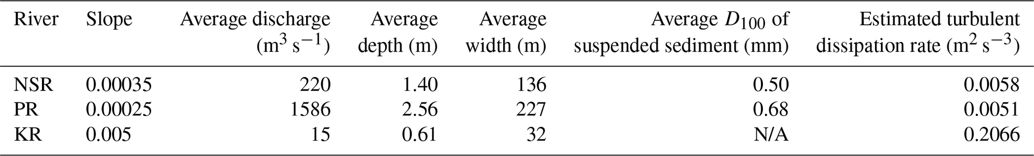
Note: slope, average discharge, average depth, and average width were obtained from Kellerhals et al. (1972); average D₁₀₀ values of suspended sediments were computed from Water Survey of Canada historic size distribution data measured at North Saskatchewan River at Edmonton (05DF001) and Peace River at Dunvegan Bridge (07FD003) (Water Survey of Canada, 2023).

Figure 1 Maps showing (a) the locations of the deployment sites in Alberta as well as enlarged views of the locations on (b) the North Saskatchewan, (c) Kananaskis, and (d) Peace rivers. These maps were produced with QGIS software (https://qgis.org/en/site/, last access: 2 January 2024) using the data provided by © OpenStreetMap contributors (https://www.openstreetmap.org/copyright, last access: 2 January 2024) and MapTiler (http://openmaptiles.org/, last access: 2 January 2024).

2 Study reaches

Measurements were conducted in three regulated Alberta rivers: the North Saskatchewan River (NSR) at Edmonton, the Peace River (PR) near Fairview, and the Kananaskis River (KR). Figure 1 shows the geographical locations of the study reaches, deployment sites, and weather stations. The characteristics of the study reaches are summarized in Table 1. The turbulent dissipation rate in Table 1 was estimated using the listed slope as well as the average depth and width following Clark and Doering (2008). The three rivers are significantly different in terms of their sizes and hydraulic characteristics. The flow of the NSR is regulated by the Brazeau and Bighorn dams, which are ∼233 and ∼423 km upstream of the Laurier Park site, respectively. A daily water level fluctuation of 0.3 to 0.4 m occurred in the study reach due to hydropeaking (McFarlane et al., 2017). The estimated turbulent dissipation rate is 0.0058 m² s⁻³. Freeze-up typically starts in early November and ends in early to late December with the formation of a static ice cover. However, the 2022 winter freeze-up progressed in a surprisingly rapid manner, starting on 5 November 2022, and ending just 3 d later on 8 November 2022.

The PR has the largest average discharge, depth, and width of the three rivers (Table 1). The estimated turbulent dissipation rate is 0.0051 m² s⁻³, which is slightly smaller than that of the NSR. The flow of the PR is regulated by the WAC Bennett Dam and the Peace Canyon Dam, which are ∼309 and ∼288 km upstream of the Fairview water intake deployment site, respectively. These outflows at the dams are relatively warm water (∼6 °C) during the winter, affecting the river's thermal regime for up to 550 km downstream of the dams (Jasek and Pryse-Phillips, 2015), which is ∼250 km downstream of the deployment site. Therefore, supercooling and frazil ice generation only occurs at the deployment site when the zero-degree isotherm is located upstream and ceases when it retreats downstream. This unique condition allows freeze-up to persist until the ice front reaches the Fairview intake site, typically in mid-January.

The KR is the smallest of the three rivers in terms of average discharge, depth, and width (Table 1). It has the largest turbulent dissipation rate, with a value of 0.2066 m² s⁻³, which is not unexpected since the KR is a small, steep river in the mountains. The flow is regulated by the Pocaterra Dam, which is 12 and 31 km upstream of the Fortress and Evan Thomas deployment sites, respectively. In winter, a dramatic discharge fluctuation from ∼1 to 21 m³ s⁻¹ occurred daily in the study reach due to hydropeaking (Government of Alberta, 2023). Low flows promote border ice formation, reducing the channel width, while high flows cause overtopping of existing ice and/or banks and prevent the formation of complete ice cover. Without ice cover to insulate the water, supercooling events and frazil generation occur when the air temperature is sufficiently cold.

Figure 2 An image showing the configuration of the FrazilCam system.

3 Instrumentation, methodology, and deployments

A submersible camera system initially designed for imaging suspended frazil ice particles and named the “FrazilCam” (McFarlane et al., 2017) was modified in this study to image frazil flocs in the water column. Figure 2 shows the modified configuration of the FrazilCam system. A 36 MP Nikon D800 DSLR camera equipped with a Micro-Nikkor 60 mm f/2.8D lens was used to image underwater frazil ice particles and flocs. The camera was enclosed in an Ikelite waterproof housing. Two 16 cm × 16 cm Cavision linear glass cross-polarizing filters were mounted 3.6 cm apart, which is 1.6 times larger than the original configuration. A PVC enclosure with a brass fitting on the top was installed in between the camera lens and polarizing filters to prevent ice or debris from flowing through this region, blocking the camera field of view (FOV). The brass fitting was used for hot-water injection to melt any ice that was initially trapped inside the enclosure. A Nikon SB-910 Speedlight flash in a Subal SN-910 waterproof housing was used as the light source, and a 5 mm thick white acrylic board was placed in between the polarizers and flash to diffuse the light. The camera settings were determined by submerging the system in a laboratory tank filled with tap water and capturing images of a transparent plastic ruler placed inside the camera FOV. This yielded an ISO of 6400, an aperture of f/25, and a shutter speed of $\mathrm{1}/\mathrm{320}$. The configuration resulted in an image scale of 25.6 µm per pixel and an average FOV of 11.6 cm by 15.6 cm, which is 6 times larger than the original configuration. The reason for enlarging the FOV and increasing the gap between the polarizers was to enable larger flocs to pass through and fit within the FOV.

Figure 3 An image showing the ice accumulation on the FrazilCam system.

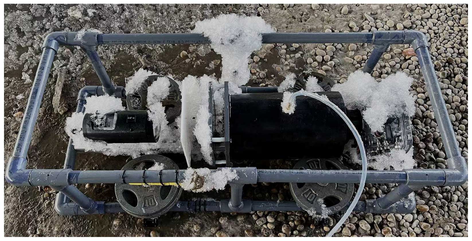
At the start of each deployment, the camera was programmed to acquire five images at 1 Hz every 9, 15, or 18 s, depending on the field conditions, until the battery was depleted. A longer sampling interval (e.g. 18 s) was chosen for some deployments to prolong the deployment duration, with the goal of capturing a complete supercooling event. Just prior to the deployment of the FrazilCam in the river, the polarizers were rinsed with hot saline water to prevent ice crystals from forming on them once submerged. The system was then quickly deployed in the river and the PVC enclosure was filled with hot fresh water from an elevated container. During deployments, anchor ice often formed on system components, as shown in Fig. 3, and ice that formed on the polarizers could obstruct the FOV of the camera. To prevent or mitigate this problem, the polarizers were inspected every 30 to 60 min and hot saline water was injected onto the polarizers to melt any ice crystals.

During each deployment, an RBR Solo T (accuracy ±0.002 °C) temperature logger sampling every second was attached to the top of the frame to measure water temperature, and a Van Essen Diver (accuracy ±1 cm H₂O) water level logger sampling every 10 min was attached to the bottom of the frame to measure the water depth (Fig. 2). The water depth during the PR deployments was measured using a wading rod since the Diver had stopped working. For all deployments, the depth-averaged water velocity was estimated using velocities measured adjacent to the FrazilCam at 60 % of the water depth. During the 2021 winter, the water velocity was measured using a 2 MHz Nortek AquaDopp high-resolution acoustic Doppler current profiler sampling every second with a blanking distance of 0.1 m and averaging every 2 min. For the rest of the deployments, the water velocity was measured using a SonTek flow tracker handheld acoustic Doppler velocimeter (ADV) sampling every second for a total duration of 50 s.

Meteorological conditions for the NSR reach were measured by a weather station installed at the EL Smith water treatment plant, which is located ∼90 m from the river bank and ∼6 km upstream of the Laurier Park site (Fig. 1b). The weather station measures the air temperature, solar radiation, relative humidity, atmospheric pressure, and wind speed and direction every minute and logs data every 10 min. An Apogee SN-500-SS net radiometer was deployed on the river bank at this location, where it measured incoming and outgoing shortwave and longwave radiation every minute and logged data every 10 min. For the PR, meteorological data were obtained at 1 h intervals from the Environmental and Climate Change Canada (ECCC) station Fairview AGDM (ID: 3072525) and cloud coverage data were obtained at 3 h intervals from the closest ECCC station, Peace River A (ID: 3075041), as shown in Fig. 1d. For the KR, the Kananaskis Boundary Auto weather station operated by Alberta Forestry, Parks and Tourism (ACIS, 2023) was used to obtain 1 h interval air temperature, humidity, wind speed, and wind direction data. In addition, 1 h solar radiation data were obtained from the University of Calgary Barrier Lake Field Station weather station (University of Calgary, 2023), and 3 h cloud coverage data were obtained from the closest ECCC station, Calgary Intl A (ID: 3031092), as shown in Fig. 1c. ECCC weather station datasets are available online (Environmental and Climate Change Canada, 2023). Table 2 summarizes the distances between weather stations and deployment sites. All weather stations are located within 30 km of their nearby deployment sites, except for those providing cloud coverage data for the PR and KR.

Table 2 The distances between weather stations and deployment sites.

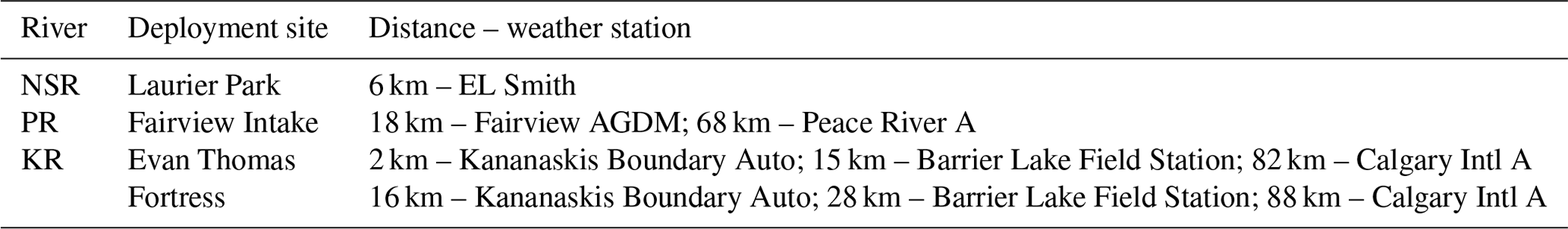
Table 3 Summary of the FrazilCam deployments and site conditions, including the number (#) of images captured, mean air temperature $\stackrel{\mathrm{‾}}{T_{\mathrm{a}}}$, mean water depth $\stackrel{\mathrm{‾}}{d}$, depth-averaged water velocity $\stackrel{\mathrm{‾}}{U}$, and local Reynolds number Re.

Figure 4 Images of the FrazilCam deployed during (a) NSR-L6 and (b) KR-E1. The arrow indicates the flow direction.

The FrazilCam system was deployed a total of 11 times during the 2021 and 2022 freeze-up periods. Images of the FrazilCam during two of the deployments are shown in Fig. 4. The image sampling protocols were five images at 1 Hz every 9 s for all NSR and KR-E1 deployments, five images at 1 Hz every 15 s for KR-F1 and KR-F2, and five images at 1 Hz every 18 s for all PR deployments. Table 3 lists the detailed location, date, time, number of images processed, and deployment number for each deployment. The mean air temperature $\stackrel{\mathrm{‾}}{T_{\mathrm{a}}}$, mean water depth $\stackrel{\mathrm{‾}}{d}$, depth-averaged flow velocity $\stackrel{\mathrm{‾}}{U}$, and the local Reynolds number Re computed from $\stackrel{\mathrm{‾}}{d}$ and $\stackrel{\mathrm{‾}}{U}$ are also presented in Table 3. Eight of the 11 deployments started in the afternoon around 14:00–19:00, when the effect of solar radiation had reduced, decreasing the heat gain of the water body. Note that all times referenced are in mountain standard time (MST). The time durations of the deployments ranged from 1 h 48 min to 3 h 21 min. As can be seen from Table 3, during these deployments, $\stackrel{\mathrm{‾}}{T_{\mathrm{a}}}$ ranged from −3.5 to −20.6 °C, $\stackrel{\mathrm{‾}}{d}$ ranged from 0.41 to 1.24 m, $\stackrel{\mathrm{‾}}{U}$ ranged from 0.12 to 0.36 m s⁻¹, and Re ranged from 44 866 to 160 714, indicating that frazil floc properties and concentrations were measured and analyzed over a wide range of meteorological and hydraulic conditions. The 11 deployments captured various phases of supercooling, but NSR-L4 was the only deployment that captured a complete principal supercooling phase (i.e., from when the water temperature first dropped below zero to when an approximately stable residual temperature was reached).

Figure 5 (a) An example of a raw FrazilCam image captured on 3 December 2021, and (b) the corresponding processed binary image.

4 Data processing

4.1 Image processing

Figure 5a shows an example of a raw FrazilCam image with individual frazil ice particles, flocs, and ice crystals frozen on the polarizer. Frazil ice particles are predominantly disc-shaped (McFarlane et al., 2017) and therefore, depending on their orientation, appear in the images as shapes that vary from a line to a circle, with the majority being ellipses. Flocs form through the aggregation of frazil ice particles, resulting in varying shapes, depending on the number, shape, and size of the attached particles. Ice crystals sometimes attached and froze to the surface of the polarizers despite the periodic hot saline-water rinsing. These crystals may appear anywhere in the image, blocking certain regions of the FOV.

Figure 6 A flow chart showing the image processing procedure.

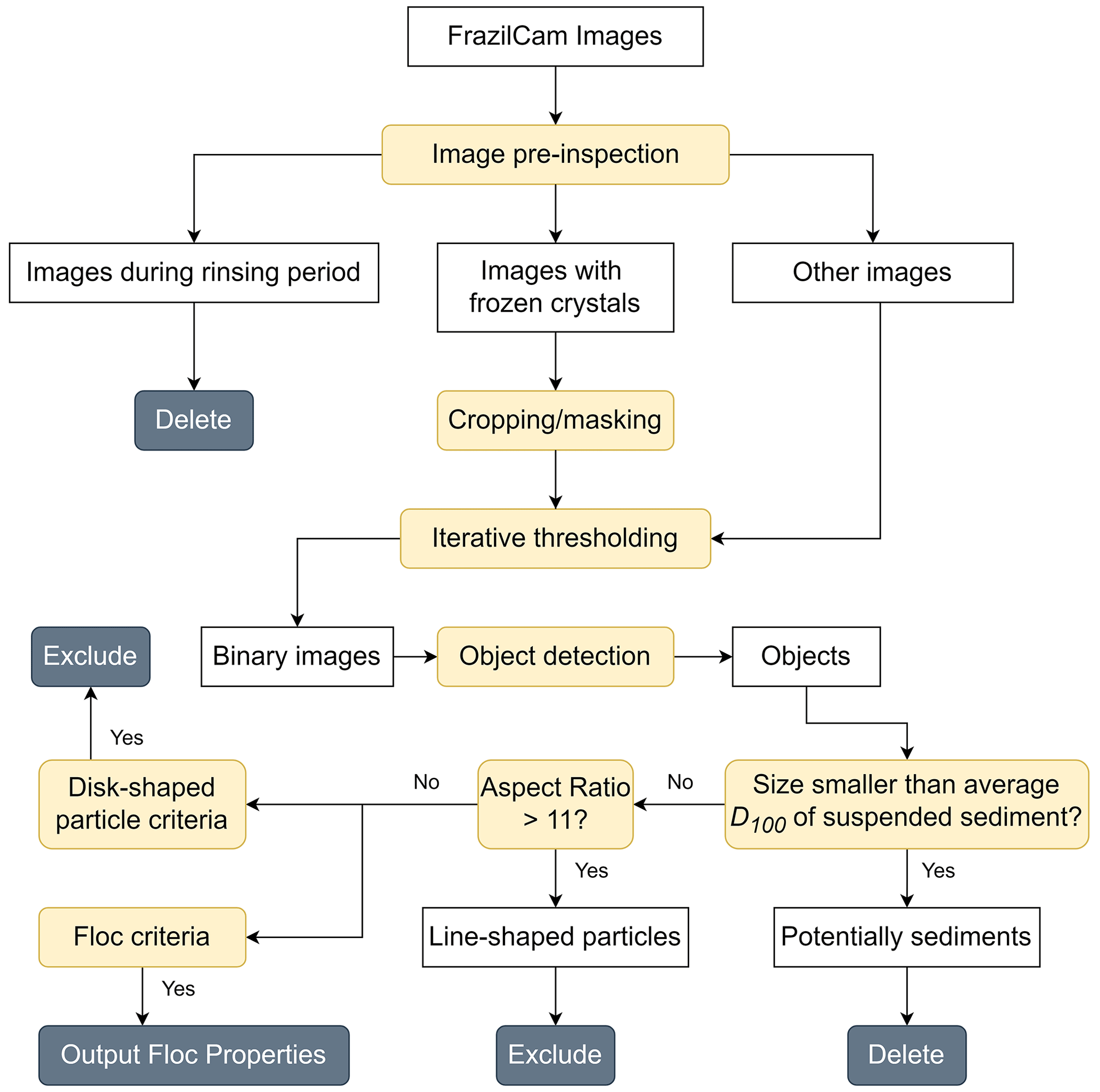
Figure 6 shows a flow chart of the image processing procedure used for extracting frazil floc properties. For each deployment, images were first manually inspected to exclude those taken when the polarizers were being rinsed, which constituted 2 %–14 % of the total number of images captured. Each image was then processed using an iterative thresholding algorithm developed by McFarlane et al. (2014) to determine the location and extent of each object. Objects intersecting with the image boundary were eliminated, which also removed the ice crystals that were frozen near polarizer edges. For frozen ice crystals that did not intersect with the image boundary, the affected image area was removed by either cropping, masking, or a combination of both (Fig. 6). The corresponding processed binary image is shown in Fig. 5b.

The processed binary images were analyzed to compute each object's basic geometric characteristics, such as its area, perimeter, and centroid as well as the major- and minor-axis lengths of its fitted ellipse. The size S of a frazil particle or floc was defined as the major-axis length of its fitted ellipse (Clark and Doering, 2009). The objects in the processed images may have included small suspended sediments that were thin enough to refract light, which may significantly distort the size distribution of frazil ice particles and flocs (McFarlane et al., 2017; Pei et al., 2022). McFarlane et al. (2019a) used a support vector machine (SVM) to distinguish between ice particles and sediments and compute accurate particle size distributions. However, this method requires ice-free sediment images at each site for site-specific SVM training, which is not possible for this study due to the lack of ice-free images at the PR and KR sites. Since this study focuses on flocs, which are considerably larger than particles, a simple cut-off criterion was used to minimize the effect of sediment particles in the images. Objects smaller than the average D₁₀₀ of suspended sediment (see Table 1) in a given study reach were removed from the dataset (Fig. 6). For the KR, since no suspended sediment size distribution measurements were available in the literature, the cut-off size was determined to be 0.27 mm, which is twice the average of seven mean sediment size measurements estimated from FrazilCam images by McFarlane et al. (2019b).

For each object, the following geometric parameters were used to classify the objects into either flocs or particles: the ratio of the object area to that of the fitted ellipse $a/a_{\mathrm{e}}$, the absolute percentage difference between the object perimeter and its fitted ellipse perimeter P_diff%, and the ratio of an object's fitted ellipse area to its ellipse perimeter divided by the ratio of the object's actual area to its perimeter $\left(\frac{a_{\mathrm{e}}}{P_{\mathrm{e}}}\right)/\left(\frac{a}{P}\right)$ (McFarlane et al., 2014; Schneck, 2018). Preliminary experiments found that flocs formed by a very small particle attaching to a significantly larger particle remain approximately elliptical since the boundary does not change significantly. As a result, comparing changes in overall area or perimeter with the fitted ellipse did not help with classification. Therefore, the form index was introduced to assess minor changes in object shape (Masad et al., 2001; Al-Rousan et al., 2007). The form index is calculated using the following equation:

$$\begin{array}{}\text{(1)}& \text{FI}=\sum _{\mathit{\theta }=\mathrm{0}}^{\mathit{\theta }=\mathrm{360}-\mathrm{\Delta }\mathit{\theta }}{\displaystyle \frac{\left|R_{\mathit{\theta }+\mathrm{\Delta }\mathit{\theta }}-R_{\mathit{\theta }}\right|}{R_{\mathit{\theta }}}},\end{array}$$

where θ is the directional angle and R is the radial length between the centroid of the particle and the boundary of the particle. The incremental change in angle Δθ is set to 2.81°, dividing the particle boundary into 128 segments to factor in minor boundary changes. A perfectly circular object has an FI of 0, and FI will increase as the object's boundary becomes more irregular.

A total of 568 objects were manually labelled as either flocs (109) or disc-shaped frazil particles (459) to construct a test dataset to determine the optimal classification criteria of the aforementioned parameters. Results showed that $\mathit{\{}a/a_{\mathrm{e}}\ge \mathrm{0.9}$ and P_diff%≤0.1 and S≤6} provided the optimum classification accuracy of 97.0 % for disc-shaped particles, and $\mathit{\left\{}\right(a/a_{\mathrm{e}}<\mathrm{0.9}$ or P_diff%>0.15) and $\left(\frac{a_{\mathrm{e}}}{P_{\mathrm{e}}}\right)/\left(\frac{a}{P}\right)>\mathrm{1.1}$ and FI≥6} provided the optimum classification accuracy of 92.7 % for flocs. In NSR-L4, the camera lens was slightly out of focus due to an accidental jarring of the camera during deployment. However, because this was the only deployment that captured a complete principal supercooling event, additional processing was performed on these images to allow for their inclusion in the dataset. Visual examination and analysis of these images indicated that the blurriness predominantly affected the boundary clarity of dim objects with a mean pixel intensity of less than 24 and did not significantly affect brighter objects. Therefore, an additional criterion was introduced for NSR-L4: flocs with a mean pixel intensity of less than 24 were eliminated. The rate of floc detection in the blurry images from deployment NSR-L4 was 4.1 flocs per minute, and it was 4.4 flocs per minute in NSR-L5, which occurred immediately afterwards. Therefore, the additional criterion applied to the blurry images only slightly reduced the number of flocs detected.

In order to prevent line-shaped frazil ice particles from being misidentified as flocs, frazil particles in the shape of a line were first identified as those for which the aspect ratio of the object (i.e., the ratio between the major- and minor-axis lengths) was greater than 11, based on minimum frazil ice particle aspect ratio measurements made by McFarlane et al. (2014), as shown in Fig. 6. Then the classification criteria mentioned above were applied to the remaining objects to identify disc-shaped particles and flocs (Fig. 6). After classification, the number of flocs N_T, mean floc size $\stackrel{\mathrm{‾}}{{\mathit{\mu }}_{\mathrm{f}}}$, standard deviation σ_f, 95th percentile of floc size S_f95, maximum floc size S_fmax, average floc number concentration $\stackrel{\mathrm{‾}}{C_{\mathrm{fn}}}$, and average volumetric concentration $\stackrel{\mathrm{‾}}{C_{\mathrm{fv}}}$ for each deployment were computed. It is worth noting that the properties of frazil ice particles were not included in this study since the cut-off size likely eliminated up to 50 % of the particle population, which would have significantly skewed the data. In addition, the mean floc size μ_f, floc number concentration C_fn, and floc volumetric concentration C_fv were computed for each image throughout a deployment, and a moving average over a period of 35 images was applied to the resulting time series to smooth the data. Note that the 35-image moving average was computed only if two or more non-zero values occurred in the window; if there were less than two non-zero values, no average value was recorded. This created gaps in the moving average time series, and the rationale for this is that two or more samples are required to compute a valid average value. The measuring volume used for the concentration calculations was the image FOV times the gap distance between the two polarizers. The volume of a frazil floc was assumed to be the volume of an ellipsoid with semi-axis lengths of a, b, and c, where a and b were equal to the semi-major- and semi-minor-axis lengths of the floc's fitted ellipse, and c was equal to the average of a and b but no larger than the gap between the two polarizing filters. The volume of ice in a frazil floc V_f was estimated as

$$\begin{array}{}\text{(2)}& V_{\mathrm{f}}={\displaystyle \frac{\mathrm{4}}{\mathrm{3}}}\mathit{\pi }abc(\mathrm{1}-\mathit{\eta }),\end{array}$$

where η is the porosity of floc, taken to be 0.8 (Schneck et al., 2019).

4.2 Heat flux analysis at the water surface

The net heat flux Q_n at the river surface is given by

$$\begin{array}{}\text{(3)}& Q_{\mathrm{n}}=Q_{\mathrm{sw}}+Q_{\mathrm{lw}}+Q_E+Q_H,\end{array}$$

where Q_sw is the net shortwave radiation, Q_lw is the net longwave radiation, Q_E is the latent heat flux, and Q_H is the sensible heat flux. A positive sign denotes heat loss from the surface. Q_sw was calculated as

$$\begin{array}{}\text{(4)}& Q_{\mathrm{sw}}=-(\mathrm{1}-{\mathit{\alpha }}_{\mathrm{ws}})Q_{\mathrm{s}},\end{array}$$

where Q_s is the measured incoming solar radiation and α_ws is the albedo of the water surface to solar radiation, taken to be 0.15 for this study, following Howley (2021). The net longwave radiation Q_lw was calculated as

$$\begin{array}{}\text{(5)}& {\displaystyle }{Q}_{\mathrm{lw}}=Q_{\mathrm{lw}}^{\mathrm{out}}-(\mathrm{1}-{\mathit{\alpha }}_{\mathrm{wl}})Q_{\mathrm{lw}}^{\mathrm{in}},\text{(6)}& {\displaystyle }{Q}_{\mathrm{lw}}^{\mathrm{out}}={\mathit{\epsilon }}_{\mathrm{w}}{\mathit{\sigma }}_{\mathrm{sb}}{T}_{\mathrm{wk}}^{\mathrm{4}},\end{array}$$

where $Q_{\mathrm{lw}}^{\mathrm{out}}$ is the outgoing longwave radiation emitted from the water; α_wl is the albedo of the water surface to longwave radiation, taken as 0.03 (Raphael, 1962); ε_w is the emissivity of water, taken as 0.97 (Ashton, 2013); σ_sb is the Stefan–Boltzmann constant ($\mathrm{5.67}\times {\mathrm{10}}^{-\mathrm{8}}$ W m⁻² K⁻⁴); and T_wk is the water surface temperature in K. Note that it was assumed that the water column was completely mixed, and therefore the water temperatures that were measured at the top of the FrazilCam frame (i.e., not at the water surface) were used in Eq. (6). $Q_{\mathrm{lw}}^{\mathrm{in}}$ is the incoming longwave radiation, which was measured by a net radiometer for the NSR. For the KR and PR, $Q_{\mathrm{lw}}^{\mathrm{in}}$ was estimated using the following equations:

$$\begin{array}{}\text{(7)}& {\displaystyle }{Q}_{\mathrm{lw}\mathrm{\_}\mathrm{c}}^{\mathrm{in}}={\mathit{\epsilon }}_{\mathrm{ac}}{\mathit{\sigma }}_{\mathrm{sb}}{T}_{\mathrm{ak}}^{\mathrm{4}},\text{(8)}& {\displaystyle }{\mathit{\epsilon }}_{\mathrm{ac}}=\mathrm{1.08}\left[\mathrm{1}-\exp (-e_{\mathrm{a}}^{T_{\mathrm{ak}}/\mathrm{2016}})\right],\text{(9)}& {\displaystyle }{e}_{\mathrm{s}}=\mathrm{6.11}\exp \left({\displaystyle \frac{\mathrm{17.62}{T}_{\mathrm{a}}}{\mathrm{243.12}+T_{\mathrm{a}}}}\right),\text{(10)}& {\displaystyle }{e}_{\mathrm{a}}=\text{RH}\times e_{\mathrm{s}},\text{(11)}& {\displaystyle }{Q}_{\mathrm{lw}}^{\mathrm{in}}=Q_{\mathrm{lw}\mathrm{\_}\mathrm{c}}^{\mathrm{in}}\left(\mathrm{1}-N^{\mathrm{4}}\right)+\mathrm{0.952}{N}^{\mathrm{4}}{\mathit{\sigma }}_{\mathrm{sb}}{T}_{\mathrm{ak}}^{\mathrm{4}},\end{array}$$

where $Q_{\mathrm{lw}\mathrm{\_}\mathrm{c}}^{\mathrm{in}}$ is the incoming longwave radiation under a clear sky; ε_ac is the clear-sky atmospheric emissivity calculated using Eq. (8) by Satterlund (1979); T_ak is the air temperature in K; e_s and e_a are the saturated and actual vapour pressure of water, respectively; RH is the relative humidity; T_a is the air temperature in degrees Celsius; and N is the fractional cloud cover. Note that Eq. (11) was developed by Konzelmann et al. (1994).

Q_E was calculated using the equation suggested by Ryan et al. (1974) following Yang et al. (2023):

$$\begin{array}{}\text{(12)}& \begin{array}{rl}{Q}_E& =\left[\mathrm{2.70}{\left({\displaystyle \frac{T_{\mathrm{wk}}}{\mathrm{1}-\mathrm{0.378}(e_{\mathrm{s}}/P)}}-{\displaystyle \frac{T_{\mathrm{ak}}}{\mathrm{1}-\mathrm{0.378}(e_{\mathrm{a}}/P)}}\right)}^{\frac{\mathrm{1}}{\mathrm{3}}}\right.\\ & \left.+\mathrm{3.2}V\right](e_{\mathrm{s}}-e_{\mathrm{a}}),\end{array}\end{array}$$

where P is the atmospheric pressure and V is the wind speed. Q_H was calculated from Q_E using Bowen's ratio B as follows:

$$\begin{array}{}\text{(13)}& {\displaystyle }B={\displaystyle \frac{C_{\mathrm{a}}P}{\mathrm{0.622}{l}_{\mathrm{v}}}}\times {\displaystyle \frac{T_{\mathrm{s}}-T_{\mathrm{a}}}{e_{\mathrm{s}}-e_{\mathrm{a}}}},\text{(14)}& {\displaystyle }{Q}_H=B{Q}_E,\end{array}$$

where C_a is the specific heat of air, l_v is the latent heat of vaporization, and T_s is the surface water temperature. In a previous study, Yang et al. (2023) investigated various formulas used to calculate the incoming longwave radiation and the latent and sensible heat fluxes during freeze-up on the North Saskatchewan River in Alberta, and the combination of formulas (Eqs. 7–14) used in this study were the ones that provided the most accurate results in Yang et al. (2023). It is also worth noting that only hourly meteorological data were available for the KR and PR regions, as described in Sect. 3. As a result, the heat fluxes were calculated at 1 h time intervals for the KR and PR deployments, and for all the NSR deployments, the heat fluxes were calculated at 10 min time intervals.

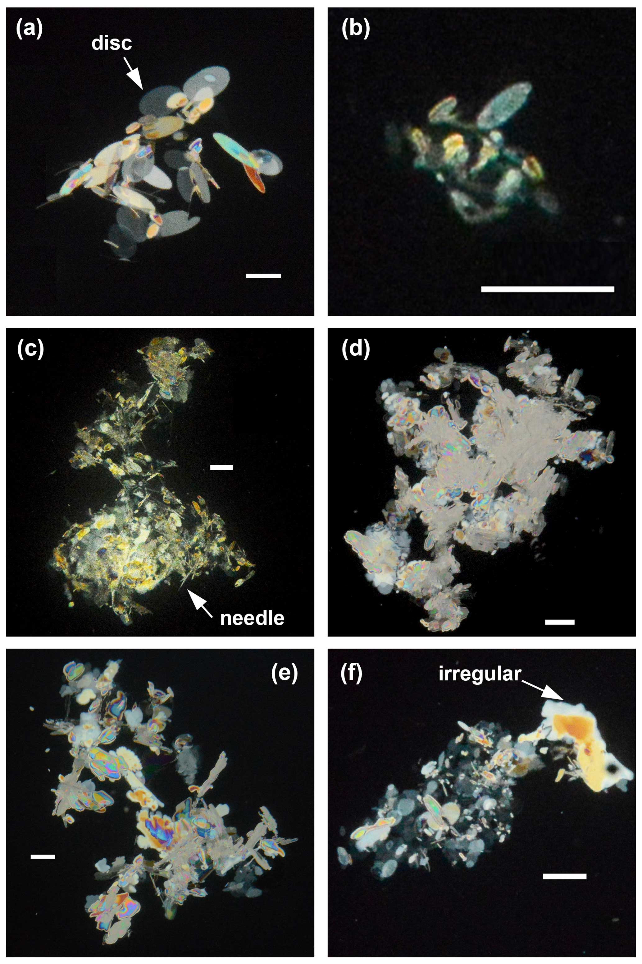
Figure 7 Images of frazil flocs of different sizes and shapes from the following deployments: (a) NSR-L1, (b) NSR-L6, (c) PR-F1, (d) KR-E1, (e) KR-F1, and (f) KR-F2. The white scale bar in each image represents a length of 3 mm. Note that in some images, the surrounding ice particles were masked out to highlight the floc at the centre of the image.

5 Results

5.1 Floc shape, size, and concentration

In Fig. 7, images of typical shapes of frazil flocs observed during the different field deployments are presented. Flocs from NSR deployments (Fig. 7a and b) were composed predominantly of disc-shaped frazil ice particles of varying sizes frozen together. The floc shown in Fig. 7b is representative of flocs observed during deployments NSR-L3 and NSR-L6. As can be seen, it was composed of much smaller individual particles than the flocs observed during the rest of the NSR deployments (Fig. 7a). Flocs from deployment PR-F1 (Fig. 7c) were composed of disc-shaped particles, irregular particles, and some needle-shaped particles. Flocs from deployment KR-E1 (Fig. 7d) were formed primarily by densely aggregated irregular particles and some small disc-shaped particles. Flocs from deployments PR-F2, KR-F1 (Fig. 7e), and KR-F2 (Fig. 7f) were mostly composed of disc-shaped and irregular particles. Images of flocs from PR-F2 are not shown since they are similar to those shown in Fig. 7e–f.

Table 4 Supercooling phase, minimum water temperature T_p, mean net surface heat flux $\stackrel{\mathrm{‾}}{Q_{\mathrm{n}}}$, number of flocs N_T, mean floc size $\stackrel{\mathrm{‾}}{{\mathit{\mu }}_{\mathrm{f}}}$, standard deviation σ_f, 95th percentile of floc size S_f95, maximum floc size S_fmax, average floc number concentration $\stackrel{\mathrm{‾}}{C_{\mathrm{fn}}}$, and average volumetric concentration $\stackrel{\mathrm{‾}}{C_{\mathrm{fv}}}$ for each deployment.

Table 4 presents the number of flocs N_T; mean size $\stackrel{\mathrm{‾}}{{\mathit{\mu }}_{\mathrm{f}}}$; standard deviation σ_f; 95th percentile and maximum of the floc size S_f95 and S_fmax, respectively; average floc number concentration $\stackrel{\mathrm{‾}}{C_{\mathrm{fn}}}$; and average volumetric concentration $\stackrel{\mathrm{‾}}{C_{\mathrm{fv}}}$ for each deployment. The supercooling phase, the minimum water temperature T_p, and average net surface heat flux $\stackrel{\mathrm{‾}}{Q_{\mathrm{n}}}$ are also presented. Deployments NSR-L1, NSR-L3, and NSR-L4 captured the principal supercooling phase (“Principal deployments”), while the rest captured only the residual supercooling phase (“Residual deployments”). T_p ranged from −0.021 to −0.031 °C for Principal deployments and from −0.007 to −0.017 °C for Residual deployments. In all deployments, $\stackrel{\mathrm{‾}}{Q_{\mathrm{n}}}$ was positive, indicating an overall heat loss. N_T varied significantly, ranging from 442 to 187 288, with the largest N_T of 187,288 occurring during deployment KR-E1. The mean floc size $\stackrel{\mathrm{‾}}{{\mathit{\mu }}_{\mathrm{f}}}$ ranged from 1.19 to 5.64 mm, with an overall average of 3.8 mm, and σ_f ranged from 0.88 to 5.03 mm. S_f95 was greater than ∼8 mm except for deployments NSR-L3 and NSR-L6, with values of 4.44 and 2.47 mm, respectively. The largest value of S_fmax, 99.69 mm, was observed during KR-E1, which also had the largest number of flocs. The average floc number concentration $\stackrel{\mathrm{‾}}{C_{\mathrm{fn}}}$ varied by 3 orders of magnitude from $\mathrm{1.80}\times {\mathrm{10}}^{-\mathrm{4}}$ to $\mathrm{1.15}\times {\mathrm{10}}^{-\mathrm{1}}$ cm⁻³, and the average floc volumetric concentration $\stackrel{\mathrm{‾}}{C_{\mathrm{fv}}}$ varied by over 4 orders of magnitude from $\mathrm{2.05}\times {\mathrm{10}}^{-\mathrm{7}}$ to $\mathrm{4.56}\times {\mathrm{10}}^{-\mathrm{3}}$.

Figure 8 Distributions of floc size S_f for deployments (a) NSR-L1, (b) NSR-L6, (c) KR-F1, and (d) PR-F1. The red line denotes a fitted lognormal distribution, N is the number of flocs in each bin, and N_T is the total number of flocs.

5.2 Floc size distribution

In Fig. 8, plots of the frazil floc size distribution as well as fitted lognormal-distribution curves for four deployments are presented. All of the size distributions obtained from NSR deployments closely resemble deployment NSR-L1 shown in Fig. 8a, except for deployment NSR-L6 shown in Fig. 8b. Size distributions from the KR and PR are well represented by deployments KR-F1 and PR-F1, which are shown in Fig. 8c and d, respectively. It can be seen from Fig. 8 that a theoretical lognormal distribution is a reasonable fit to all of the size distributions but a particularly good fit for deployment KR-F1. This may be attributed to the order-of-magnitude larger sample size for KR-F1 (23 670) compared to NSR-L1 (2428) and PR-F1 (2250). The size distribution for NSR-L6 shown in Fig. 8b has the most flocs of the four deployments plotted, with a sample size of 143 097, but it does not fit a lognormal distribution as closely as the others. This is because the distribution was cut off at 0.5 mm to eliminate sediment particles. A similar condition can also be observed for PR-F1 (shown in Fig. 8d), where the cut-off was 0.68 mm. Note that the cut-offs were applied to all size distributions but only impacted the distribution significantly if a significant number of smaller flocs were detected.

Figure 9 Time series of (a) water temperature T_w and air temperatureT_a, (b) heat flux Q, (c) mean floc size μ_f, (d) floc number concentration C_fn, and (e) floc volumetric concentration C_fv for deployment NSR-L4 on 12 December 2021. The vertical dashed grey line indicates the time when the peak supercooling temperature was achieved.

Figure 10 Time series of (a) water temperature T_w and air temperature T_a, (b) heat flux Q, (c) mean floc size μ_f, (d) floc number concentration C_fn, and (e) floc volumetric concentration C_fv for deployment KR-F1 on 30 January 2023.

Figure 11 Time series of (a) water temperature T_w and air temperature T_a, (b) heat flux Q, (c) mean floc size μ_f, (d) floc number concentration C_fn, and (e) floc volumetric concentration C_fv for deployment PR-F2 on 13 December 2022.

5.3 Time series

Time series plots of water temperature T_w and air temperature T_a, heat flux Q, mean floc size μ_f, floc number concentration C_fn, and floc volumetric concentration C_fv for deployments NSR-L4, KR-F1, and PR-F2 are presented in Figs. 9, 10, and 11, respectively (note that similar time series plots for the other eight deployments are presented in Figs. S1–S8 in the Supplement). Deployment NSR-L4 occurred during the principal supercooling phase and is the only deployment that captured the entire principal supercooling phase, while KR-F1 and PR-F2 captured the middle and end of the residual supercooling phase, respectively.

During NSR-L4 (Fig. 9a), supercooling started at 15:25. After that, T_w decreased almost linearly at a cooling rate of −0.0009 °C min⁻¹, reached a T_p of −0.031 °C (i.e., peak supercooling) at 16:02, and then started to increase, reaching a stable residual temperature of −0.010 °C at 16:37. T_a decreased from −1.7 to −7.2 °C, with an average of −4.6 °C. Figure 9b shows that the net heat flux Q_n increased from 26 to 150 W m⁻², primarily due to the decrease in the magnitude of shortwave radiation Q_sw. The rest of the heat flux components remained positive (heat loss) and relatively stable throughout the deployment, with Q_lw being the dominant component. In Fig. 9c, μ_f begins to increase significantly ∼7 min before the peak supercooling temperature is reached, reaching a maximum of 7.8 mm ∼37 min after peak supercooling; it then decreases to ∼6 mm and remains approximately constant afterwards. Figure 9d shows that significant numbers of frazil particles were detected ∼15 min before peak supercooling, with C_fn values below $\mathrm{2}\times {\mathrm{10}}^{-\mathrm{4}}$ cm⁻³. At ∼2 min before peak supercooling, C_fn increased rapidly, peaking ∼30 min after peak supercooling at a value of $\mathrm{9.3}\times {\mathrm{10}}^{-\mathrm{4}}$ cm⁻³, and then decreased to $\mathrm{2}\times {\mathrm{10}}^{-\mathrm{4}}$ cm⁻³ at the end of the deployment. Figure 9e shows that C_fv only increased notably after peak supercooling and reached a value of $\mathrm{8.8}\times {\mathrm{10}}^{-\mathrm{6}}$ ∼30 min after the peak supercooling. After that, it decreased before spiking to $\mathrm{1.6}\times {\mathrm{10}}^{-\mathrm{5}}$ ∼38 min after the peak supercooling and then decreased to $\mathrm{1.7}\times {\mathrm{10}}^{-\mathrm{6}}$ at the end. An examination of the images showed that the spike was caused by several large flocs up to 18.5 mm in size.

During KR-F1, T_w fluctuated continuously around −0.008 °C, except for one anomalous spike that occurred at 17:03 (Fig. 10a), which was caused by ice contacting the sensor when the polarizers were being rinsed. Additionally, periodic upward spikes with a period of 1 min and magnitude of ∼0.001 °C were visible on the plot. While the cause of these spikes remains uncertain, it is worth noting that their magnitude falls within the range of accuracy of the sensor. The air temperature was relatively stable, with T_a varying between −10 to −12 °C. In Fig. 10b, Q_n rose during the deployment from −2 to 261 W m⁻², largely due to the decrease in the magnitude of Q_sw. Note that the heat flux components were computed here at a 1 h time interval. In Fig. 10c–e, there are gaps in the data during the time periods 15:33–15:38, 16:17–16:23, 16:58–17:04, and 17:34–17:39 that are visible as short time-series segments with zero slope. These were created when the images collected during the time periods when the polarizers were being rinsed were removed from the dataset. In Fig. 10c, μ_f fluctuates around ∼4 mm before significantly increasing at 17:40, eventually reaching 5.9 mm by the end of the deployment. Similar trends are evident in Fig. 10d–e for C_fn and C_fv, respectively. At 17:41, C_fn started to increase significantly and reached a peak value of $\mathrm{4.5}\times {\mathrm{10}}^{-\mathrm{2}}$ cm⁻³ at 17:53, while C_fv started to increase significantly at 17:50 and eventually peaked at a value of $\mathrm{2.8}\times {\mathrm{10}}^{-\mathrm{3}}$. A hydropeaking wave arrived at the Fortress site at 17:25, increasing the depth by 19 % by the end of the deployment and causing rapid increases in floc size and concentration.

During deployment PR-F2, T_w was initially at −0.006 °C but increased above zero at 10:21 and eventually reached 0.033 °C at the end of the deployment (Fig. 11a). T_a followed a similar trend to T_w, rising from −7.6 to −4.1 °C. The net heat loss Q_n steadily decreased from 165 to 12 W m⁻² (Fig. 11b) due to an increase in the magnitude of Q_sw. In Fig. 11c, μ_f fluctuated between 1 and 10 mm during the deployment, with an average of 4 mm. In Fig. 11d–e, the time series of number concentration and volume concentration do not exhibit significant trends. C_fn ranged from $\mathrm{4.1}\times {\mathrm{10}}^{-\mathrm{5}}$ to $\mathrm{2.4}\times {\mathrm{10}}^{-\mathrm{3}}$ cm⁻³, with an average of $\mathrm{5.6}\times {\mathrm{10}}^{-\mathrm{4}}$ cm⁻³, while C_fv was negligible most of the time, with occasional spikes up to $\mathrm{4.2}\times {\mathrm{10}}^{-\mathrm{4}}$. One spike that occurred at 10:39 caused both C_fn and C_fv to reach their peak values. Visual examination of the images shows that at this time, the number of flocs increased significantly for three consecutive images, and this was possibly caused by a large floc colliding with the camera frame and fracturing.

6 Discussion

Images of typical frazil flocs shown in Fig. 7 illustrate the complexity of their morphology, which encompasses various ice crystal shapes, including disc-shaped, needle-shaped, and irregular particles. Disc-shaped ice particles were observed in flocs from all three rivers but were most pronounced in the NSR, where the flocs were almost all formed by disc-shaped particles of different sizes (Fig. 7a, b). The growth of frazil ice in supercooled water is limited by the diffusive removal of the latent heat of solidification from the ice–water interface and by the slow attachment kinetics in the perpendicular direction, which leads to the formation of disc-shaped particles (Mullins and Serkerka, 1964; Rees Jones and Wells, 2015). Flocs containing needle-shaped crystals as shown in Fig. 7c were observed during deployment PR-F1, which had a very low mean air temperature of −20.64 °C. These types of crystals have been found to form primarily at the surface of supercooled water (Hallett, 1960; Clark and Doering, 2002). The cold air temperature during deployment PR-F1 may have promoted the growth of these needle-shaped particles at the water surface before they were entrained in the water column and subsequently attached to flocs. Irregular particles were observed in flocs from both the KR and PR (most pronouncedly in deployment KR-E1, as shown in Fig. 7d). Irregularly shaped particles are formed by unstable disc growth, which is known to be caused by the formation of temperature gradients in the water surrounding the particles (Kallungal and Barduhn, 1977). This suggests that during the KR and PR deployments, frazil ice particles probably spent some time in relatively quiescent water, where the turbulence intensity was so low that temperature gradients could form in the water surrounding the particles. Another possibility is that the particles were temporarily transported to the river surface, exposing them to cold air, which may also lead to unstable disc growth. In addition, broken fragments of skim ice or border ice that were entrained into the water column are another possible source of irregular particles in flocs. Clark and Doering (2009) observed in the laboratory that flocs could become denser over time when the turbulence intensity was higher. During deployment KR-E1, although the locally measured depth-averaged velocity near the FrazilCam was relatively low at 0.22 m s⁻¹, the water velocity ∼70 m upstream of the deployment site was visually observed to be very turbulent due to the presence of four groins and a narrow channel width. This may have contributed to the denser flocs that were observed during this deployment.

The data presented in Table 4 and Fig. 8 are the first quantitative measurements of frazil floc sizes and concentrations in rivers. The mean floc size averaged over all deployments was 3.80 mm, which was close to the mean values observed for most of the individual deployments except for deployments NSR-L3, NSR-L6, and KR-E1, which had mean floc sizes of 1.87, 1.19, and 5.64 mm, respectively. As noted in Sect. 5.1, flocs observed during deployments NSR-L3 and NSR-L6 were composed of much smaller disc-shaped individual particles (Fig. 7b) than the rest of the deployments (Fig. 7a). Deployment NSR-L3 took place during a principal supercooling event in which the observed small frazil ice particles were likely newly formed and still growing, which could be the reason why the flocs were smaller and composed of significantly smaller particles. In addition, deployment NSR-L3 took place as the crest of a hydropeaking wave was passing the site, resulting in a mean water depth of 1.24 m, which is 37 % to 55 % larger than the depths during the other NSR deployments (Table 3). The significantly higher water depth reduced the fractional height at which the images were collected, which could also result in smaller floc sizes. This would be consistent with measurements by Reimnitz et al. (1993) that showed that larger flocs have higher rise velocities. Deployment NSR-L6 occurred during the 2022 freeze-up season, which was the shortest freeze-up in ∼10 years, lasting only 3 d. Significantly smaller flocs were observed during this deployment (see Fig. 7b), and this may be because relatively young smaller flocs were generated during this rapid freeze-up process. The largest mean floc size, maximum floc size, and concentration (see Table 4) were observed during deployment KR-E1 (Fig. 7d). As discussed previously, the particles that formed flocs during KR-E1 included irregularly shaped particles, and this could have resulted in larger flocs compared to flocs formed entirely by disc-shaped particles.

The mean floc size and standard deviation ranged from 1.19 to 5.64 mm and from 0.88 to 5.03 mm, respectively, as shown in Table 4. The 95th percentile of floc size ranged from 2.47 to 14.28 mm, and the largest floc found was 99.69 mm in size. Schneck et al. (2019) conducted laboratory experiments in a frazil ice tank with an average turbulent dissipation rate of 0.034 m² s⁻³, which falls within the range of the values estimated in the three rivers in this study (0.005–0.207 m² s⁻³). They found that in freshwater, the size distribution of flocs followed a lognormal distribution, and the mean size, 95th percentile of floc size, and maximum size were 2.57, 6.91, and 95.1 mm, respectively. The mean and 95th percentile sizes fall within the range of values observed in this study. However, the overall mean floc size observed in the field was 3.80 mm, which is 48 % larger than the mean measured in the laboratory. The maximum floc sizes observed in the laboratory and field are comparable. It is worth noting that the largest floc size of 99.69 mm was just slightly smaller than the FOV dimensions and considerably larger than the 3.6 cm gap, indicating that the floc size measurements may have been physically limited by the FOV and the gap between the polarizers. Therefore, further increases in both the FOV and the gap between the polarizers may be needed in future studies to allow even larger flocs to be imaged and measured.

The size distributions obtained from different rivers are all a reasonable visual fit to a lognormal distribution, as shown in Fig. 8, which is consistent with the laboratory measurements (Schneck et al., 2019). However, when the chi-square test for goodness of fit was applied, none of the size distributions were quantitatively confirmed to fit a lognormal distribution at the 5 % significance level. This could be primarily due to the use of the cut-off size to eliminate sediment particles which produced a sharp cut-off in the distributions. In addition, the small number of samples in some deployments resulted in noisy size distributions, making it unlikely that they would be a good quantitative fit to a smooth lognormal distribution. Nonetheless, the qualitatively good correspondence of the floc size distributions measured in the field with theoretical lognormal distributions in Fig. 8 does suggest that if the sample size was larger and sediment particles could be filtered out, floc size distributions in rivers would also closely follow a lognormal distribution.

The average floc number concentration $\stackrel{\mathrm{‾}}{C_{\mathrm{fn}}}$ ranged from $\mathrm{1.80}\times {\mathrm{10}}^{-\mathrm{4}}$ to $\mathrm{1.15}\times {\mathrm{10}}^{-\mathrm{1}}$ cm⁻³ (Table 4). Schneck et al. (2019) measured a peak floc number concentration of $\mathrm{2.5}\times {\mathrm{10}}^{-\mathrm{1}}$ cm⁻³ in freshwater laboratory experiments, which is similar in magnitude to the upper limit of values measured in the field. The average floc volumetric concentration $\stackrel{\mathrm{‾}}{C_{\mathrm{fv}}}$ ranged from $\mathrm{2.05}\times {\mathrm{10}}^{-\mathrm{7}}$ to $\mathrm{4.56}\times {\mathrm{10}}^{-\mathrm{3}}$ (Table 4). Previous studies reported suspended-ice volumetric concentrations ranging from $\mathrm{2}\times {\mathrm{10}}^{-\mathrm{6}}$ to $\mathrm{6}\times {\mathrm{10}}^{-\mathrm{3}}$ (Tsang, 1984; Marko and Jasek, 2010; Richard et al., 2011). These measurements were made using comparative-resistance probes and acoustic devices, which in theory detect all of the ice suspended in the water. The upper range of previous concentration measurements is comparable to that reported in this study. However, the lower range is 1 order of magnitude larger than this study, which may be due to the fact that the previous studies reported the total volume of frazil flocs and particles.

The time series of frazil floc properties in Fig. 9 indicate that during the principal supercooling phase, floc number, and mean size started to increase significantly just prior to peak supercooling and reached a maximum near the end of principal supercooling, whereas the floc volumetric concentration only started to increase significantly after peak supercooling occurred. Deployment NSR-L3, which captured almost the entire principal supercooling phase, also showed a similar trend (see Fig. S3). The increasing trends in the mean floc size and the floc number concentration generally agree with previous laboratory measurements (Schneck et al., 2019; Pei et al., 2023). However, the laboratory-measured mean floc size and floc number concentration stopped increasing significantly shortly after peak supercooling, while they stopped increasing later in the field – near the end of the principal supercooling phase. For example, Schneck et al. (2019) observed that the mean floc size and the floc number concentration in freshwater stopped increasing significantly at dimensionless times of $t/t_{\mathrm{c}}=\mathrm{1.13}$ and 1.27, respectively, compared to $t/t_{\mathrm{c}}=\mathrm{2.00}$ and 1.81 for NSR-L4 (t_c is the time interval between the start of supercooling and peak supercooling, and t is the time). The peak floc number concentration measured during the three principal deployments in this study ranged from $\mathrm{9.3}\times {\mathrm{10}}^{-\mathrm{4}}$ to $\mathrm{3.1}\times {\mathrm{10}}^{-\mathrm{3}}$ cm⁻³, more than 2 orders of magnitude lower than the $\mathrm{2.5}\times {\mathrm{10}}^{-\mathrm{1}}$ cm⁻³ measured in the laboratory tank by Schneck et al. (2019). These significantly lower floc concentrations suggest that particle concentrations in the field were also much lower compared to laboratory measurements. At lower suspended-frazil concentrations, the collision frequency of frazil particles would be reduced, increasing the time needed for flocs to gain mass via collision-induced particle–floc aggregation, which might explain the longer time period over which the mean floc size and the floc number concentration were observed to increase in the field.

Figure 10 shows that during KR-F1, the mean floc size was approximately constant prior to the arrival of the hydropeaking wave during the residual supercooling phase. Similarly, there were no observed trends in floc size in five other residual deployments: NSR-L2, NSR-L5, KR-E1, PR-F1 (see Figs. S2, S4, S7, and S6), and PR-F2 (Fig. 11). McFarlane et al. (2019b) found that in rivers, the mean particle size remained approximately constant during the residual supercooling phase if the environmental conditions were relatively stable. Therefore, it follows that flocs observed during the residual supercooling phase would also have a stable mean size unless hydraulic and/or meteorological conditions changed significantly. The mean floc size was most stable during deployment KR-E1 (Fig. S7), with a fluctuation range of only 1.5 mm, which could be in part due to the significantly larger sample size of 187 288. The only two residual deployments that did not have a stable mean floc size were NSR-L6 and KR-F2 (Figs. S5 and S8), and in both cases the size decreased, and this coincided with minor increases in T_w (∼0.005 °C). These results indicate that during the residual phase, the mean floc size does not typically vary significantly – even at the end of the supercooling event, when T_w rises above zero, as was the case in PR-F1 and PR-F2. During the two PR deployments, the floc properties did not change significantly during the 1.3 and 2.5 h time periods between the end of supercooling and the end of measurements. This is likely because the zero-degree isotherm had moved upstream of the deployment site but the frazil being generated upstream of it was still advecting past the FrazilCam (i.e., the zero-degree isotherm was not so far upstream that the advecting frazil had time to melt.)

As shown in Fig. 10, during KR-F1, the residual supercooling water temperature remained mostly approximately constant at approximately −0.01 °C. An approximately constant residual supercooling temperature was also observed in NSR-L2, KR-E1, and NSR-L5 (see Figs. S2, S7, and S4). This means that during the residual supercooling phase ice was still growing and releasing latent heat that balanced the heat loss from the water surface in order to maintain the approximately constant water temperature. In this study, although the mean floc size did not vary significantly during most of the measured residual supercooling deployments, fluctuations and trends in the floc number and volume concentration time series were observed. These indicate that these frazil ice particles may have still been forming and growing, releasing latent heat to help balance the surface heat loss. In addition, during the residual phase, anchor ice, border ice, and surface ice pans were likely also growing and releasing latent heat, helping to maintain the stable residual supercooling temperature.

The time series of water temperature T_w and net heat flux Q_n provided an opportunity to theoretically estimate the total ice growth in the water column, which could be compared to the measured floc volumetric concentration C_fv to estimate the fraction of ice sampled by the FrazilCam. Assuming there were no significant water temperature gradients in any direction (i.e., the river had a uniform temperature) and that the water depth was constant, the thermal balance of the water–ice mixture is given by

$$\begin{array}{}\text{(15)}& \mathit{\rho }{C}_p{\displaystyle \frac{\mathrm{d}{T}_{\mathrm{w}}}{\mathrm{d}t}}=-{\displaystyle \frac{Q_{\mathrm{n}}}{\stackrel{\mathrm{‾}}{d}}}+{\mathit{\rho }}_{\mathrm{i}}{L}_{\mathrm{i}}{\displaystyle \frac{\mathrm{d}{C}_{\mathrm{i}}}{\mathrm{d}t}},\end{array}$$

where ρ is the water density, C_p is the specific heat of water, ρ_i is the ice density, L_i is the latent heat of fusion of ice, and C_i is the total ice concentration due to thermal growth (Souillé et al., 2023). Equation (15) was then used to estimate C_i for deployment NSR-L4, which captured the entire principal supercooling phase. The result showed that the FrazilCam was only sampling at most 2 % of the total ice that was forming in the water. It should be noted that the Q_n used in the calculation does not account for the effect of surface ice due to a lack of accurate surface ice data. In addition, the mean water depth $\stackrel{\mathrm{‾}}{d}$ was used, while in reality the water depth varied spatially and temporally. These approximations create considerable uncertainty in the calculations of the total heat loss from the surface and the volume of the water being cooled. Given all the simplifying assumptions that were made, the uncertainty in the calculated C_i is potentially quite large but is likely not greater than a factor of 2 or 3. Therefore, despite this potential large uncertainty, the calculations suggest that the FrazilCam was only sampling less than ∼5 % of the total ice being formed in the river. Similar calculations were also performed using data collected in a laboratory frazil ice tank experiment using the laboratory version of the FrazilCam. In the laboratory environment, the water depth is a constant, the tank has been shown to be well mixed, and the surface heat loss can be quantified from the water cooling rate with reasonable accuracy. These results showed that C_i calculated using Eq. (15) was comparable to the volumetric concentration of suspended ice calculated from the FrazilCam images prior to when flocs began rising to the surface. This demonstrates that the FrazilCam does provide accurate measurements of the suspended-ice concentrations. However, the only time the FrazilCam would be sampling a significant fraction of the total ice being formed in a river would be when suspended frazil is the only ice that is actively growing.

The effect of the surface heat flux on floc properties was investigated. A positive mean net heat flux $\stackrel{\mathrm{‾}}{Q_{\mathrm{n}}}$ was observed for all deployments, indicating a net heat loss from the surface. The magnitude of $\stackrel{\mathrm{‾}}{Q_{\mathrm{n}}}$ ranged from 95.4 to 318.8 W m⁻², as shown in Table 4. The dominant positive heat flux was Q_lw and Q_H for six and five deployments, respectively, while the dominant negative heat flux in all deployments was Q_sw, which is consistent with previous studies (McFarlane and Clark, 2021; Boyd et al., 2023). Efforts were made to correlate the mean net heat flux $\stackrel{\mathrm{‾}}{Q_{\mathrm{n}}}$ with the measured floc properties listed in Table 4 (i.e., columns 5–11). No significant correlations were found when using data from all deployments or when only the data from the six NSR deployments that have 10 min heat flux data were used. It is worth noting that the heat flux analysis in this study did not account for varying surface ice concentrations and neglected several heat fluxes (e.g. sediment–water). Clearly, more comprehensive and frequent measurements of heat fluxes and surface ice properties are needed in future studies to more fully understand the impact of varying heat fluxes on frazil floc properties.

Figure 12 Relationship between the local Reynolds number Re and mean floc size $\stackrel{\mathrm{‾}}{{\mathit{\mu }}_{\mathrm{f}}}$ in mm.

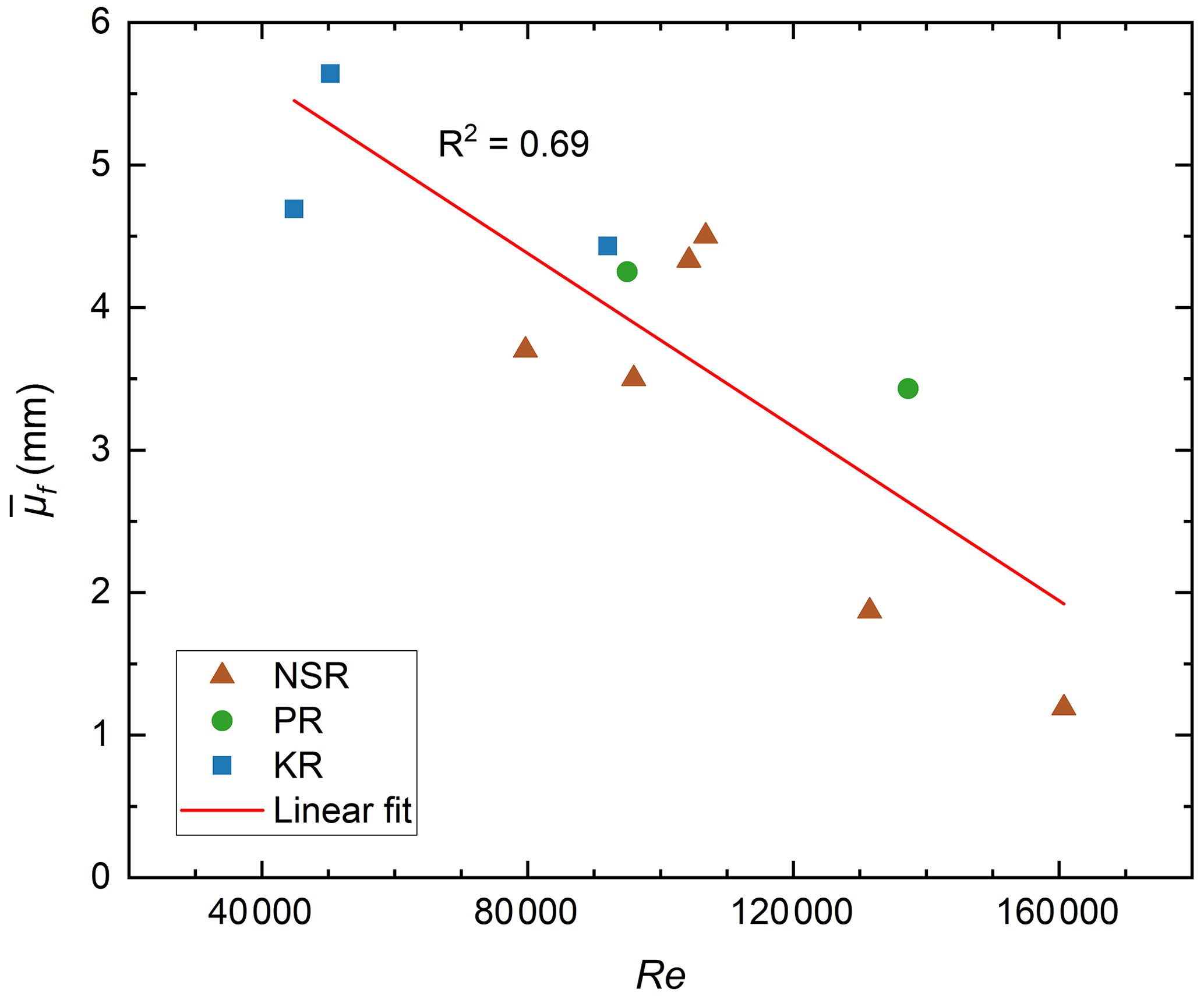
To investigate the effect of hydraulic conditions on the mean floc size μ_f, the local Reynolds number Re is plotted versus $\stackrel{\mathrm{‾}}{{\mathit{\mu }}_{\mathrm{f}}}$ in Fig. 12 along with the following linear-regression equation:

$$\begin{array}{}\text{(16)}& \stackrel{\mathrm{‾}}{{\mathit{\mu }}_{\mathrm{f}}}=\mathrm{6.82}-\mathrm{3.05}\times {\mathrm{10}}^{-\mathrm{5}}\mathit{Re}.\end{array}$$

As Re increases from ∼40 000 to ∼160 000, $\stackrel{\mathrm{‾}}{{\mathit{\mu }}_{\mathrm{f}}}$ decreases from approximately 5.5 to 2 mm and the coefficient of determination (R²) is 0.69, indicating that the two are moderately correlated. Clark and Doering (2009) found that a higher turbulence intensity inhibited the formation of large flocs. This finding is consistent with the correlation presented in Fig. 12 if it is assumed that turbulence intensity increased with Re in the three study rivers. However, this is not necessarily the case. An alternate explanation for the observed correlation is that as Re increased, the flocs experienced higher shear strain rates (i.e., larger velocity gradients) and more violent floc–floc collisions, which would tend to rupture larger flocs and reduce their mean size.

Figure 13 Relationship between the fractional height $d_{\mathrm{m}}/\stackrel{\mathrm{‾}}{d}$ and the average floc volumetric concentration $\stackrel{\mathrm{‾}}{C_{\mathrm{fv}}}$.

The effect of water depth on the floc volumetric concentration was investigated by correlating the average volumetric concentration with the fractional height $d_{\mathrm{m}}/\stackrel{\mathrm{‾}}{d}$, where d_m=0.198 m is the height above the bed at the centre of the FrazilCam FOV and $\stackrel{\mathrm{‾}}{d}$ is the mean water depth. Figure 13 presents a scatter plot of the fractional height $d_{\mathrm{m}}/\stackrel{\mathrm{‾}}{d}$ versus the average floc volumetric concentration $\stackrel{\mathrm{‾}}{C_{\mathrm{fv}}}$. Results show that there is a strong nonlinear correlation given by the following power law equation:

$$\begin{array}{}\text{(17)}& \stackrel{\mathrm{‾}}{C_{\mathrm{fv}}}=\mathrm{4.80}{\left({\displaystyle \frac{d_{\mathrm{m}}}{\stackrel{\mathrm{‾}}{d}}}\right)}^{\mathrm{9.69}},\end{array}$$

where the R² value equals 0.99. Ye (2002) and Morse and Richard (2009) reported measurements of vertical frazil concentration profiles and found that the Rouse equation (Rouse, 1937), previously used to characterize suspended-sediment concentration profiles, could be used to describe the frazil ice concentration profile. Equation (17) is similar in format to the Rouse equation, indicating that the vertical concentrations of both frazil particles and flocs may be accurately described by power law equations.

7 Conclusions

A submersible high-resolution camera system was deployed during supercooling in three rivers from 2021–2023. Images from the 11 deployments were analyzed to investigate frazil floc properties and their evolution. Images showed that frazil flocs observed in the North Saskatchewan River were predominately formed by disc-shaped particles, while flocs in the Peace River and Kananaskis River were composed of various ice crystal shapes, including disc-shaped, needle-shaped, and irregular particles. A lognormal distribution is a reasonable description of the floc size distributions in rivers. The mean floc size ranged from 1.19 to 5.64 mm and the overall mean floc size was 3.80 mm. The mean floc size in rivers was found to be 48 % larger than was previously observed in the laboratory by Schneck et al. (2019), while the maximum floc sizes in the laboratory and field were comparable. The average floc number concentration ranged from $\mathrm{1.80}\times {\mathrm{10}}^{-\mathrm{4}}$ to $\mathrm{1.15}\times {\mathrm{10}}^{-\mathrm{1}}$ cm⁻³, and previous laboratory measurements fall within the range of the values observed in this study. The estimated average floc volumetric concentration ranged from $\mathrm{2.05}\times {\mathrm{10}}^{-\mathrm{7}}$ to $\mathrm{4.56}\times {\mathrm{10}}^{-\mathrm{3}}$, with the upper bound being comparable to previous total ice volume concentration measurements while the lower bound is an order of magnitude smaller.

Time series analysis indicated that during the principal supercooling phase, floc number concentration and mean size increased significantly just before peak supercooling and reached a maximum near the end of principal supercooling. This increasing trend was also observed in previous laboratory measurements (Schneck et al., 2019; Pei et al., 2023), but the duration of the increasing trend was longer in the field. During the residual supercooling phase, the mean floc size did not typically vary significantly, even 2.5 h after the water temperature rose above 0 °C. The effect of the air–water heat flux on floc properties was investigated by conducting a linear-regression analysis. However, no significant correlations were found, and this may be due to the limited dataset or the complexity of the field environment, where heat fluxes can vary temporally and spatially. Future field measurements of floc properties, especially those made during the principal supercooling phase and made continuously along multiple sites along a study reach, are needed to more fully understand the factors that govern their size and concentration.

Analysis of the influence of local hydraulic conditions on frazil floc properties showed that as the local Reynolds number increases, the mean floc size decreases linearly. The resulting equation can be used to estimate mean floc sizes in rivers using estimates of the mean velocity and depth. It was also shown that the averaged floc volumetric concentration can be related to the fractional height above the bed through a power law equation. This relationship may be useful for describing the vertical concentration profiles of frazil flocs.

The detailed measurements of frazil floc properties and their evolution in rivers presented in this study could be used in several ways to enhance the numerical modelling of river ice processes in order to improve predictions of river freeze-up. At the present time, the frazil rise velocity is treated as a calibration parameter in comprehensive river ice process models (e.g. Shen, 2010; Blackburn and She, 2019). However, it could now be directly estimated by first using Eq. (16) to predict the mean floc size using the local Reynolds number, and then the rise velocity could be predicted using the measurements in Reimnitz et al. (1993). In addition, the reported lognormal size distributions of flocs as well as the time series evolutions of the mean floc size and the concentrations, measured in rivers for the first time, could provide opportunities to incorporate floc dynamics into numerical models with the goal of improving how realistically they simulate frazil ice evolution and surface ice progression.

In the future, it would be of interest to deploy the FrazilCam in lakes and oceans, where the flow regime and salinity may be considerably different, to investigate frazil particle and floc properties in these different environments. The FrazilCam system can, in principle, be deployed in any sufficiently transparent waters; however, the system would need to be modified to automate the polarizer rinsing process. This would be challenging but might be possible using a mechanical wiper, which would allow deployments on the bottom of deeper water bodies. In addition, the system could be attached to an uncrewed or autonomous underwater vehicle to allow observations to be made at various depths in the water column in lakes and oceans.