Assessing sea ice microwave emissivity up to submillimeter waves from airborne and satellite observations

Upcoming submillimeter wave satellite missions require an improved understanding of sea ice emissivity to separate atmospheric and surface microwave signals under dry polar conditions. This work investigates hectometer-scale observations of airborne sea ice emissivity between 89 and 340 GHz, combined with high-resolution visual imagery from two Arctic airborne field campaigns that took place in summer 2017 and spring 2019 northwest of Svalbard, Norway. Using k-means clustering, we identify four distinct sea ice emissivity spectra that occur predominantly across multiyear ice, first-year ice, young ice, and nilas. Nilas features the highest emissivity, and multiyear ice features the lowest emissivity among the clusters. Each cluster exhibits similar nadir emissivity distributions from 183 to 340 GHz. To relate hectometer-scale airborne measurements to kilometer-scale satellite footprints, we quantify the reduction in the variability of airborne emissivity as footprint size increases. At 340 GHz, the emissivity interquartile range decreases by almost half when moving from the hectometer scale to a footprint of 16 km, typical of satellite instruments. Furthermore, we collocate the airborne observations with polar-orbiting satellite observations. After resampling, the absolute relative bias between airborne and satellite emissivities at similar channels lies below 3 %. Additionally, spectral variations in emissivity at nadir on the satellite scale are low, with slightly decreasing emissivity from 183 to 243 GHz, which occurs for all hectometer-scale clusters except those predominantly composed of multiyear ice. Our results will enable the development of microwave retrievals and assimilation over sea ice in current and future satellite missions, such as the Ice Cloud Imager (ICI) and EUMETSAT Polar System – Sterna (EPS–Sterna).

1 Introduction

Passive microwave observations from polar-orbiting satellites have continuously monitored polar regions with high spatial coverage for over 5 decades (Comiso and Hall, 2014). These observations are essential for atmosphere (e.g., Triana-Gómez et al., 2020; Perro et al., 2020), sea ice (e.g., Spreen et al., 2008; Kilic et al., 2020; Soriot et al., 2023), and joint atmosphere–sea-ice retrievals (e.g., Scarlat et al., 2020; Rückert et al., 2023; Kang et al., 2023). Such satellite-based retrievals help us to understand the accelerated Arctic near-surface warming compared to the global mean (Rantanen et al., 2022; Wendisch et al., 2023). However, the highly variable sea ice emissions cause uncertainties in satellite retrievals and severely limit the use of surface-sensitive microwave channels in operational numerical-weather-prediction data assimilation compared to the open ocean (Lawrence et al., 2019). Therefore, current research aims to improve the assimilation of microwave observations over sea ice; for example, Bormann (2022) showed improved performance occurs when Lambertian rather than specular reflection is assumed in forward simulations.

Further spaceborne capabilities will become available through the novel Ice Cloud Imager (ICI; Buehler et al., 2007) and EUMETSAT Polar System – Sterna (EPS–Sterna; Albers et al., 2023) instruments, which will feature operational channels above 200 GHz for the first time. These channels provide higher sensitivity to small cloud ice particles than current passive microwave sensors (Buehler et al., 2012; Wang et al., 2017a; Eriksson et al., 2020). However, variable emissions from polar surfaces also significantly contribute to the atmospheric signal received at the 243 (ICI only) and 325 GHz channels due to the dry atmosphere (Wang et al., 2017b).

While there is considerable interest in expanding sea ice emissivity estimates to account for submillimeter waves, few field observations cover this frequency range. The first brightness temperature (TB) observations of sea ice at 220 GHz were obtained using an airborne cross-track scanning radiometer (Hollinger et al., 1984). However, sea ice emissivity was derived only at lower frequencies, up to 140 GHz, due to high TB noise and low atmospheric transmissivity at 220 GHz during the field study. The observations revealed similar nadir emissivities at 90 and 140 GHz, with higher emissivity over young ice (0.96) and lower emissivity over multiyear ice (0.68). Airborne observations with along-track scanning radiometers from Hewison and English (1999) provide detailed emissivity spectra for typical sea ice types and snow from 24 to 157 GHz and demonstrate the importance of volume scattering within snow at 157 GHz. Hewison et al. (2002) calculated the nadir emissivities of sea ice from 24 to 183 GHz at different development stages, from new ice to multiyear ice, using similar instrumentation to that used in Hewison and English (1999). New-ice emissivities were highest at 89 GHz, measuring 0.95, and slightly decreased to 0.9 at 183 GHz. First-year ice emissivities decreased from 24 to 157 GHz and slightly increased from 157 to 183 GHz. This emissivity increase at higher frequencies was also found for multiyear ice. Haggerty and Curry (2001) observed first-time emissivities of up to 243 GHz at nadir at a resolution of ∼1 km². However, leads, which are typically smaller, could not be resolved. The 340 GHz channel aboard the same aircraft was insensitive to surface emission due to low atmospheric transmissivity. Airborne observations by Wang et al. (2017b) measured sea ice emissivities of up to 325 GHz, revealing high spatial variability, but the driving sea ice properties at this frequency could not be estimated.

While field studies demonstrate the high sensitivity of microwaves to sea ice and snow properties in limited regions, only global sea ice emission information allows for atmospheric retrievals from satellites. As modeling sea ice emissions is computationally expensive and requires detailed knowledge of sea ice and snow properties (Royer et al., 2017; Picard et al., 2018; Rückert et al., 2023), which is missing on global scales, spaceborne emissivity climatologies have been developed (Wang et al., 2017b; Munchak et al., 2020). The Tool to Estimate Land Surface Emissivity from Microwave to Submillimeter Waves (TELSEM2; Wang et al., 2017b) climatology for sea ice and land surfaces extrapolates emissivities up to 700 GHz to provide first-guess emissivities for upcoming satellite missions, such as ICI. To simultaneously retrieve atmospheric, sea ice, and snow properties, radiative-transfer models of sea ice and atmosphere have been combined (Rückert et al., 2023; Kang et al., 2023). Kang et al. (2023) additionally simulated sea ice growth to increase the temporal consistency of the retrieved sea ice and snow properties. However, sea ice radiative-transfer models might only be valid below 100 GHz. Recently, observed snow emissivities (up to 243 GHz) were successfully simulated based on realistic snow properties (Wivell et al., 2023). This result highlights the need for similar sea ice emissivity field observations that account for submillimeter waves to improve future modeling studies of sea ice. These field observations must also be related to satellite observations, which resolve the surface at a much coarser resolution.

The limitation of sea ice emissivity observations at the scale of submillimeter waves and their relevance for future satellite missions motivate our study, which is structured around two objectives. First, we aim to identify critical physical sea ice and snow properties affecting emissivity up to submillimeter wavelengths, as observed during two airborne field campaigns. We calculate the sea ice emissivity from TBs at 89 (25° incidence angle; horizontal polarization), 183, 243, and 340 GHz (nadir) using the airborne Microwave Radar/radiometer for Arctic Clouds (MiRAC; Mech et al., 2019). Then, we characterize typical emissivity spectra with airborne visual imagery and surface temperature observations. Second, we aim to relate the observed hectometer-scale emissivity observations to the satellite scale. This includes an assessment of emissivity variability as a function of footprint size. Furthermore, we collocate MiRAC with observations from polar-orbiting satellites and analyze spectral variations in emissivity observed at satellite resolutions from 89 to 340 GHz, relevant for upcoming satellite missions (such as ICI and EPS–Sterna).

The paper is outlined as follows. Section 2 describes the airborne field data, microwave instruments, and auxiliary data. Section 3 details the emissivity calculation. Section 4 identifies relevant sea ice and snow properties that affect emissivity pertaining to airborne observations. Section 5 compares emissivity levels between airborne and satellite observations, and the study is summarized and concluded in Sect. 6.

2 Data

2.1 Field data

We use airborne observations from two campaigns: Arctic CLoud Observations Using airborne measurements during polar Day (ACLOUD), from 23 May to 26 June 2017 (Wendisch et al., 2019; Ehrlich et al., 2019b), and Airborne measurements of radiative and turbulent FLUXes of energy and momentum in the Arctic boundary layer (AFLUX), from 19 March to 11 April 2019 (Mech et al., 2022a). Both campaigns were conducted as part of the “Arctic Amplification: Climate Relevant Atmospheric and Surface Processes and Feedback Mechanisms” ((AC)³) research project (Wendisch et al., 2023). The research flights (RFs) with the Polar 5 aircraft (Wesche et al., 2016) from the Alfred Wegener Institute, Helmholtz Centre for Polar and Marine Research (AWI), covered the Fram Strait, located northwest of Svalbard, Norway (Fig. 1). Polar 5 carried MiRAC (a microwave package), the KT-19 (a thermal infrared sensor), and a visual camera, as well as other instruments. Various sea ice characteristics were observed with Polar 5 during the ACLOUD campaign (i.e., during RF23 on 25 June and RF25 on 26 June 2017) and the AFLUX campaign (i.e., during RF08 on 31 March, RF14 on 8 April, and RF15 on 11 April 2019) under clear-sky conditions and over sea ice suitable for emissivity estimation. During the two ACLOUD flights, melt ponds formed on the sea ice, and there was open water between individual ice floes. During the three AFLUX flights, snow-covered sea ice, mostly composed of multiyear ice (Fig. A1), prevailed, with nilas found in refrozen leads between individual ice floes. Higher fractions of open water during the AFLUX campaign were only observed in the marginal sea ice zone of RF08. The infrared-based mean surface temperatures were near the freezing point, ranging from 0.8 to 1 °C during both ACLOUD flights, and well below the freezing point, ranging from −22 to −17 °C during the three AFLUX flights. The integrated water vapor, derived from in situ observations (see Sect. 2.4), was about 10 to 10.3 kg m⁻² during the two ACLOUD flights and 1.3 to 2 kg m⁻² during the three AFLUX flights, which indicates reduced water vapor emissions and high atmospheric transmissivity during the AFLUX campaign.

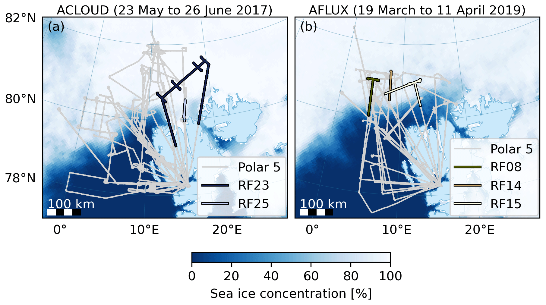
Figure 1 All Polar 5 flights, clear-sky segments over sea ice, and mean sea ice concentrations (Spreen et al., 2008) during (a) the ACLOUD campaign, from 23 May to 26 June 2017, and (b) the AFLUX campaign, from 19 March to 11 April 2019.

2.2 Airborne microwave instruments

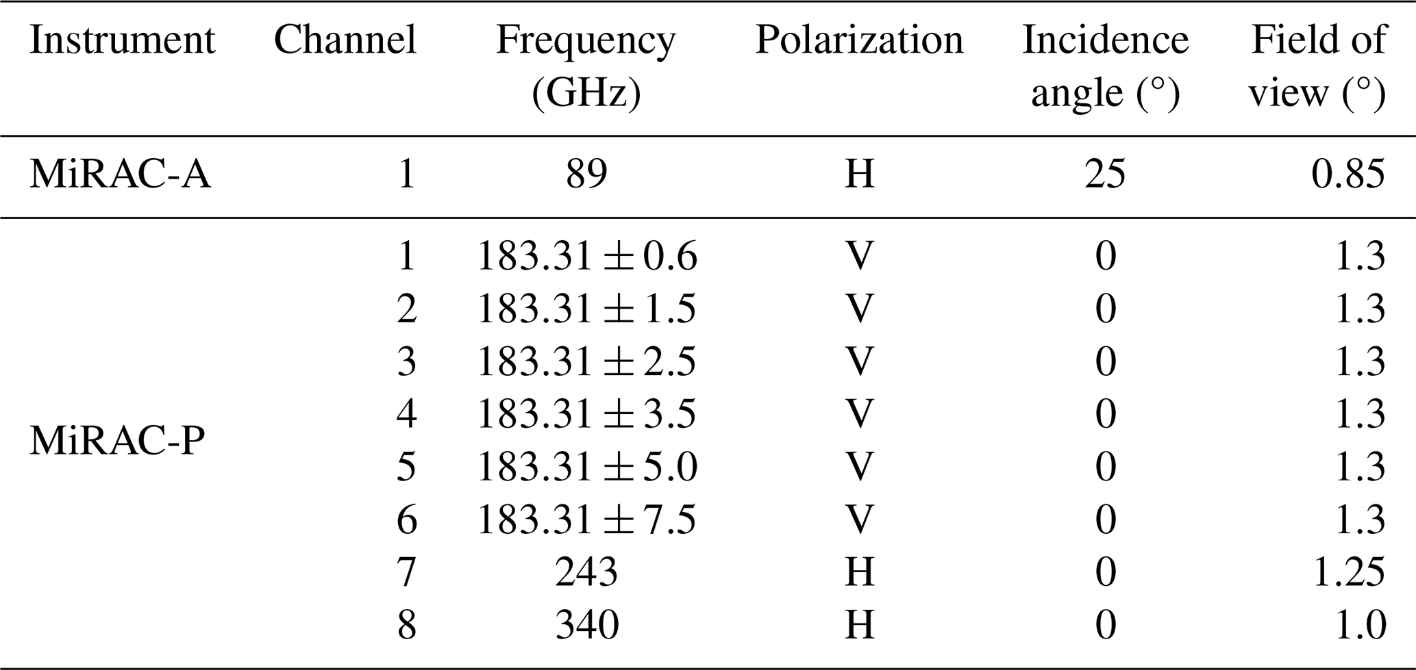
Polar 5 carried the MiRAC package, which includes the combined active–passive component (MiRAC-A), mounted inside a belly pod beneath the aircraft's fuselage, and the solely passive component (MiRAC-P), deployed inside the aircraft cabin (Mech et al., 2019). MiRAC-A consists of a 94 GHz cloud radar and a passive 89 GHz channel with horizontal polarization, measuring backward with a 25° incidence angle. MiRAC-P measures at six double-sideband water vapor channels (183.31±0.6, ±1.5, ±2.5, ±3.5, ±5.0, and ±7.5 GHz) and two window channels (243 and 340 GHz) at nadir (see Table 1). Both MiRAC components measure at a temporal resolution of 1 s. We exclude MiRAC-A observations collected during low flights, i.e., when the slant path between the instrument and the surface is less than 500 m, due to contamination resulting from back-scattered broadband noise from the cloud radar. This threshold means MiRAC-A is entirely excluded during ACLOUD RF25, where the flight altitude during clear-sky transects over sea ice ranges from 60 to 350 m. For the other four flights, the typical flight altitudes range from 60 m to 3 km, with about 80 % (15 %) of the time spent below 500 m (above 2.5 km). Furthermore, we exclude observations with aircraft roll or pitch angles above 10°. The flight distance over which MiRAC provides emissivities depends on the channel, ranging from 400 km at 89 GHz to 1,700 km at 243 GHz. For about 200 km of this distance, all MiRAC-A and MiRAC-P channels provide emissivities nearly instantaneously – i.e., the spatially matched footprint centers of MiRAC-P and the inclined MiRAC-A are less than 200 m apart.

The instrument receivers were calibrated with a two-point calibration using liquid nitrogen and an internal target at the beginning of each campaign. In addition, MiRAC-A performed gain calibrations every 15 min (and MiRAC-P performed them every 20 min) during flights using an internal target (Mech et al., 2019). After the campaign, we applied a bias correction to the 89 GHz TBs, following Konow et al. (2019); this was based on Passive and Active Microwave radiative TRAnsfer (PAMTRA; Mech et al., 2020) forward simulations and used dropsonde profiles under clear-sky conditions over the open ocean, extended by ERA5 reanalysis (Hersbach et al., 2020) to the top of the atmosphere, and a sea surface temperature analysis (UK Met Office, 2012) as inputs. The added 89 GHz TB offset for the ACLOUD (AFLUX) flights in this study is 11 (32) K and decreases linearly toward higher TBs. This high calibration offset occurred due to difficult weather conditions during the liquid-nitrogen calibration. We estimate the accuracy of the offset correction to be 2 K. For MiRAC-P, no such calibration issues occurred due to its location inside the aircraft cabin (Mech et al., 2019). The TB noise is about 0.5 K for MiRAC-A (Küchler et al., 2017) and MiRAC-P (Mech et al., 2019), indicating an upper bound of the observed TB noise of 0.2 to 0.3 K, based on a homogeneous time series during ACLOUD RF10. This random noise cancels out when averaging, but we do not consider this here as systematic effects dominate the overall emissivity uncertainty (see Sect. 3.2). Hence, we assume the overall TB uncertainty from bias correction and noise to be 2.5 K at 89 GHz and 0.5 K at all other frequencies. The footprint size at a 60 m s⁻¹ flight velocity with a 1 s integration time is about 70×130 m² at 3 km flight altitude and 1×60 m² at 60 m flight altitude at 183 GHz, i.e., at nadir with an opening angle of 1.3° (see Table 1). We shift the MiRAC measurement time by 1 to 2 s (2 to 5 s) during the ACLOUD (AFLUX) campaign relative to the infrared radiometer KT-19 as determined from lagged correlations between 243 GHz TBs and KT-19 infrared TBs during the clear-sky sea ice emissivity flight segments. Note that the 243 GHz channel showed the highest correlation with the infrared TB of all MiRAC-P channels during both campaigns due to its high atmospheric transmission compared to the other MiRAC-P channels.

Table 1 Specifications of the passive MiRAC-A and MiRAC-P channels. H: horizontal. V: vertical.

2.3 Satellite microwave instruments

We focus on commonly used cross-track and conical polar-orbiting scanning microwave radiometers. These include the Microwave Humidity Sounder (MHS; EUMETSAT, 2010), the Advanced Technology Microwave Sounder (ATMS; Kim et al., 2014), the Special Sensor Microwave Imager/Sounder (SSMIS; Kunkee et al., 2008), and the Advanced Microwave Scanning Radiometer 2 (AMSR2; JAXA, 2016); their platforms and specifications are summarized in Table 2. To ensure consistency among the sensors, we use intercalibrated Level 1C TB data (NASA Goddard Space Flight Center and GPM Intercalibration Working Group, 2022). This intercalibration corrects offsets between the constellation satellites using the well-calibrated Global Precipitation Measurement (GMP) Microwave Imager (GMI) (Hou et al., 2014), which covers up to 65° N, as a reference (Berg et al., 2016).

MHS and ATMS conduct cross-track scanning at incidence angles of up to 59 and 64°, respectively, and the SSMIS and AMSR2 scan conically at incidence angles of 53 and 55°, respectively. MHS and ATMS measure TBs with nominal vertical (QV) or nominal horizontal (QH) polarization at nadir, rotating with view angle α. These TBs are expressed as

$$\begin{array}{}\text{(1)}& T_{\mathrm{b},\mathrm{QV}}=T_{\mathrm{b},\mathrm{V}}{\cos }^{\mathrm{2}}\left(\mathit{\alpha }\right)+T_{\mathrm{b},\mathrm{H}}{\sin }^{\mathrm{2}}\left(\mathit{\alpha }\right)\end{array}$$

and

$$\begin{array}{}\text{(2)}& T_{\mathrm{b},\mathrm{QH}}=T_{\mathrm{b},\mathrm{H}}{\cos }^{\mathrm{2}}\left(\mathit{\alpha }\right)+T_{\mathrm{b},\mathrm{V}}{\sin }^{\mathrm{2}}\left(\mathit{\alpha }\right),\end{array}$$

respectively. We only use MHS and ATMS data with incidence angles from 0 to 30° because these angles provide observation conditions similar to those of MiRAC. Moreover, fewer footprints with higher incidence angles collocate with MiRAC, and their increased footprint sizes make comparisons more uncertain. Using this incidence angle filter for MHS and ATMS, the footprint sizes are mostly around 16×16 km², with the highest resolution of 3×5 km² provided by AMSR2. MHS aboard the NOAA-18 spacecraft only operated during the ACLOUD campaign, and the Metop-C and NOAA-20 spacecraft only operated during the AFLUX campaign. The 150 GHz channel of the SSMIS aboard the DMSP-F18 satellite was unavailable due to its failure (Berg et al., 2016).

MiRAC overlaps spectrally with MHS, ATMS, and SSMIS at 89 and 183 GHz and overlaps spectrally with AMSR2 at 89 GHz. However, MiRAC's 89 GHz channel, which measures under horizontal polarization at 25°, is not directly comparable with the satellite channels because MHS and ATMS mostly measure vertically polarized TBs near this incidence angle, and SSMIS and AMSR2 measure at higher incidence angles. Only MiRAC's 183 GHz near-nadir channel is directly comparable with near-nadir observations from MHS and ATMS.

Table 2 Specifications of the MHS, ATMS, SSMIS, and AMSR2 channels used in this study. The instantaneous field of view (IFOV) from MHS and ATMS is given for nadir observations. The polarizations for MHS and ATMS are either nominal vertical (QV) at nadir, rotating with the view angle, or nominal horizontal (QH) at nadir, rotating with the view angle. The polarizations for SSMIS and AMSR2 are either horizontal (H) or vertical (V). Only 0–30° incidence angles from MHS and ATMS are used here.

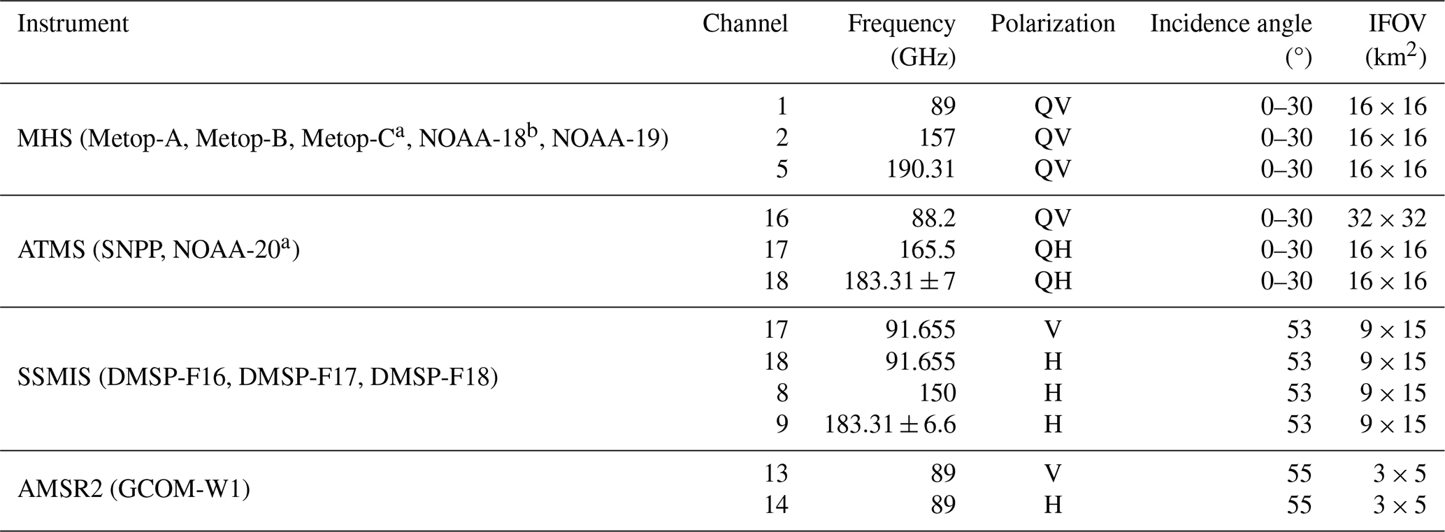
^a Satellite only operated during the AFLUX campaign. ^b MHS aboard NOAA-18 only operated during the ACLOUD campaign

2.4 Ancillary observations

The emissivity retrieval requires ancillary information on the atmospheric thermodynamic profile and surface temperature. We construct the thermodynamic profile below 3 km altitude from measurements of the aircraft's nose boom and dropsondes, and we construct the thermodynamic profile above 3 km altitude from radiosondes (Maturilli, 2020) launched at the AWIPEV station, operated jointly by the AWI and the Polar Institute Paul-Emile Victor (IPEV) in Ny-Ålesund, Svalbard, Norway (Neuber, 2003). If no dropsonde information is available over sea ice, we assume constant temperature and humidity from the lowest flight altitude of about 100 m down to the surface. The air temperature measured at these heights differs by less than 5 K from the mean surface temperature, which indicates that the profiles capture typical Arctic surface temperature inversions (e.g., Tjernström and Graversen, 2009). The uncertainties in temperature and relative humidity are ±0.2 K and ±2 % for dropsondes (Vaisala, 2010), ±0.2–0.4 K and ±3–4 % for radiosondes (Maturilli, 2020), and ±0.3 K and ±0.4 % for the nose boom (Ehrlich et al., 2019b).

The KT-19 aboard Polar 5 provides infrared TBs integrated over the atmospheric window from 9.6 to 11.5 µm, with a 1 s resolution and an opening angle of 2° at nadir. Hence, its opening angle is slightly larger than MiRAC's opening angles. The accuracy of the KT-19 is about ±0.5 K. The infrared TBs are converted to surface skin temperatures with an infrared emissivity of 0.995, similar to Høyer et al. (2017) and Thielke et al. (2022), which approximates the infrared emissivity of typical sea ice types and oceans with an accuracy of 0.01 to 0.02 (Hori et al., 2006). We use the KT-19 data as input for the sea ice emissivity calculation for MiRAC. We also require an accurate description of the surface temperature at the satellite footprint scale, which has higher spatial coverage than the KT-19. Therefore, we use the daily “Arctic Ocean – Sea and Ice Surface Temperature” reanalysis (Level 4) with a resolution of 0.05×0.05° (Nielsen-Englyst et al., 2023), which matches the AMSR2 satellite footprint size (hereafter referred to as NE23). The product derives daily gap-free sea and ice surface temperatures from clear-sky thermal infrared satellite observations sensitive to the upper few millimeters of snow or ice (Warren, 1982) and passive microwave-based sea ice concentrations. A comparison between the airborne surface temperatures based on the KT-19 and the NE23 temperatures reveals biases of 4 to 6 K during the ACLOUD campaign and biases of -1 to 1 K during the AFLUX campaign (KT-19 minus NE23). During the ACLOUD campaign, the KT-19 temperatures are close to the melting point, which agrees with observed melting conditions and a snow liquid water fraction of around 15 % (Rosenburg et al., 2023). We use the nearest NE23 ice surface temperature pixel to the satellite footprint as input for the sea ice emissivity calculation for satellites. Furthermore, a downward-looking camera equipped with a fish-eye lens operating in the visible spectrum (red, green, and blue) aboard Polar 5 provides information on sea ice characteristics every 4 to 6 s. Finally, three data products contribute surface information: daily sea ice concentration maps from the University of Bremen with a 6.25×6.25 km² resolution, based on AMSR2 (Spreen et al., 2008); daily wintertime multiyear ice concentration maps from the University of Bremen with a 12.5×12.5 km² resolution, based on AMSR2 and the Advanced Scatterometer (ASCAT; Melsheimer and Spreen, 2022); and Sentinel-2B Level 2A (L2A) visual images with a 20×20 m² resolution (European Space Agency, 2021). Although the multiyear ice concentration product incorporates microwave observations from AMSR2 and ASCAT that may correspond to observations collected at MiRAC frequencies, the implemented temperature and drift corrections increase independence between multiyear ice concentration and MiRAC TB.

We utilize topographic data from the Norwegian Polar Institute to exclude observations over land and near the coastline (Norwegian Polar Institute, 2014). Specifically, we exclude data within 150 m of the shoreline for MiRAC and within about one footprint radius of 2.5 km (8 km) for AMSR2 (MHS, ATMS, and SSMIS).

2.5 Collocation of MiRAC with satellites

To compare MiRAC with satellites, we require nearly simultaneous and spatially aligned observations. We achieve simultaneous observations by filtering collocations within a ±2 h window, which maximizes the number of satellite overpasses and minimizes the effects of sea ice drift. The sea ice drift during the flights is less than 1 km h⁻¹, based on data from the National Snow and Ice Data Center (NSIDC; Tschudi et al., 2020), and spatial variability exceeds temporal variability (not shown). Furthermore, we spatially align MiRAC with the nearest satellite footprints for each satellite overpass by imposing specific criteria: a footprint center distance threshold of about one footprint radius, corresponding to 2.5 km (8 km) for AMSR2 (MHS, ATMS, and SSMIS), and a minimum of 17 (50) MiRAC footprints within the AMSR2 (MHS, ATMS, or SSMIS) footprint. The latter criterion translates to a straight flight distance exceeding approximately 20 % of the satellite footprint diameter (10 % for ATMS at 89 GHz).

The number of satellite overflights during the ACLOUD (AFLUX) campaign with collocated footprints from MHS, ATMS, SSMIS, and AMSR2 is 15 (23), 0 (8), 11 (26), and 2 (9), respectively. We matched channels near 89 GHz with MiRAC-A, and channels above 100 GHz were matched with MiRAC-P. The number of satellite footprints collocated with MiRAC at 89 GHz during the ACLOUD (AFLUX) campaign is 87 (86), 0 (34), 107 (175), and 23 (159) for MHS, ATMS, SSMIS, and AMSR2, respectively. The number of satellite footprints collocated with MiRAC above 100 GHz during the ACLOUD (AFLUX) campaign is 222 (138), 0 (46), and 277 (261) for MHS, ATMS, and SSMIS, respectively. Around 70 MiRAC footprints fall within each of the satellite footprints at 89 GHz, and about 200 fall within each satellite footprint at frequencies above 100 GHz. The difference is mainly related to the higher resolution of AMSR2 at 89 GHz.

3 Methodology

3.1 Effective sea ice emissivity calculation

We directly derive effective sea ice emissivity from observed clear-sky TBs and infrared-based skin temperatures, following Prigent et al. (1997). Typically, the skin temperature differs from the temperature of the emitting sea ice or snow layer (Tonboe, 2010). The depth of the emitting layer, or penetration depth, depends on sea ice and snow properties and decreases with increasing frequency (Tonboe et al., 2006). Emissivity based on skin temperature is commonly referred to as effective emissivity, but hereafter, we use the term “emissivity” for better readability.

Harlow (2011) compared methods for estimating emitting-layer temperature from 183 GHz observations. However, their applicability to our data is limited by the absence of simultaneous downwelling 183 GHz TB measurements and uncertainties in the atmospheric profile impacting surface temperature estimates. Other studies employ precalculated penetration depths and observed sea ice temperature profiles for specific ice types (Mathew et al., 2008, 2009), which do not apply to the diverse sea ice conditions presented here.

The emissivity calculation is based on nonscattering radiative transfer (RT), which is valid under clear-sky conditions. The TB observed at aircraft or satellite height, denoted as T_b, is given by

$$\begin{array}{}\text{(3)}& T_{\mathrm{b}}=T_{\mathrm{s}}\cdot e\cdot t+T_{\mathrm{b}}^{\downarrow }\cdot t\cdot (\mathrm{1}-e)+T_{\mathrm{b}}^{\uparrow },\end{array}$$

where e represents surface emissivity, T_s represents surface temperature, t represents atmospheric transmissivity in the viewing direction between the surface and the aircraft/satellite height, $T_{\mathrm{b}}^{\downarrow }$ represents downwelling atmospheric radiation at the surface, and $T_{\mathrm{b}}^{\uparrow }$ represents upwelling atmospheric radiation at the observation height. Solving Eq. (3) for the surface emissivity yields

$$\begin{array}{}\text{(4)}& e={\displaystyle \frac{T_{\mathrm{b}}-T_{\mathrm{b}}^{\uparrow }-T_{\mathrm{b}}^{\downarrow }\cdot t}{(T_{\mathrm{s}}-T_{\mathrm{b}}^{\downarrow })\cdot t}}.\end{array}$$

Equation (4) can be solved using two RT simulations with e=0 and e=1 (Mathew et al., 2008). The solution is expressed as

$$\begin{array}{}\text{(5)}& e={\displaystyle \frac{T_{\mathrm{b}}-T_{\mathrm{b}}(e=\mathrm{0})}{T_{\mathrm{b}}(e=\mathrm{1})-T_{\mathrm{b}}(e=\mathrm{0})}}.\end{array}$$

We perform RT simulations for the Polar 5 or satellite height using PAMTRA. In PAMTRA, we select the Rosenkranz (1998) gas absorption with modifications for water vapor continuum absorption (Turner et al., 2009). We simulate specular and Lambertian reflections separately.

Satellite-based emissivity studies typically limit the emissivity calculation to channels with high atmospheric transmissivity. Using aircraft, we can increase transmissivity by flying at low altitudes. However, in addition to transmissivity, the contrast between surface temperature and atmospheric downwelling TB dominates the surface sensitivity, i.e., the sensitivity of the observed TB to emissivity changes. This can be seen when calculating the partial derivative from Eq. (3), given as follows:

$$\begin{array}{}\text{(6)}& {\displaystyle \frac{\partial T_{\mathrm{b}}}{\partial e}}=(T_{\mathrm{s}}-T_{\mathrm{b}}^{\downarrow })\cdot t=T_{\mathrm{b}}(e=\mathrm{1})-T_{\mathrm{b}}(e=\mathrm{0}).\end{array}$$

This term corresponds to the denominator in Eq. (5) and should be maximized to avoid noisy emissivity estimates. We identify 40 K as a reasonable threshold below which emissivity noise exceeds typical signatures of sea ice. Observed mean surface sensitivities during the AFLUX campaign are 200 K (50 K) at 89 GHz (340 GHz). Only observations obtained at 183 and 340 GHz during the ACLOUD campaign fall below the surface sensitivity threshold and are excluded to avoid highly uncertain emissivity estimates.

3.2 Emissivity uncertainty estimation

We estimate the emissivity uncertainty by propagating errors from TB (see Sect. 2.2), air temperature, relative humidity, and surface temperature. The assumed uncertainties for air temperature and relative humidity are ±2 K and ±5 %, respectively. These assumed uncertainties are higher than the dropsonde and radiosonde uncertainties to account for representability errors along the flight path. The assumed uncertainty in surface temperature is ±3 K during the ACLOUD campaign and ±8 K during the AFLUX campaign. The surface temperature uncertainty pertaining to the ACLOUD campaign mainly accounts for errors in infrared emissivity and KT-19 measurement uncertainty. The higher uncertainty in surface temperature during the AFLUX campaign, compared to the ACLOUD campaign, accounts for the spread between surface skin temperature and emitting-layer temperature, which can deviate by up to 10 K at 89 GHz over multiyear ice due to insulating snow (Tonboe, 2010). During the ACLOUD campaign, we expect mostly isothermal sea ice due to surface melt (Perovich et al., 1997). The uncertainty estimation is performed only on aircraft data, not on satellite observations, because the MiRAC channels already include most satellite channels. A notably higher emissivity uncertainty occurs for satellites operating near 183 GHz than for MiRAC, due to the higher atmospheric contributions.

3.3 Surface reflection model

The surface reflection model affects the direction from which downwelling atmospheric radiation is reflected at the surface. Typically, the surface is approximated as either purely specular or Lambertian. Across specular surfaces, the incidence angle matches the reflection angle, whereas Lambertian surfaces exhibit isotropic and unpolarized reflection. High sensitivity to the assumed surface reflection type occurs at nadir, where MiRAC conducts measurements, and low sensitivity occurs at incidence angles between 50 to 60°, where imagers like SSMIS and AMSR2 conduct measurements (Matzler, 2005; Karbou and Prigent, 2005).

Guedj et al. (2010) presented a method for constraining the surface reflection model at 50 GHz sounding channels by combining TB measurements with an emissivity retrieval. They calculated the emissivity at a wing channel of the absorption line to simulate an adjacent inner channel, finding Lambertian reflection across Antarctica in winter and seasonal variations in specular contributions. Here, we adapt the method to 183 GHz MiRAC observations collected during the three AFLUX flights by following three steps. First, we calculate emissivities at 183.31±7.5 GHz under both specular and Lambertian reflection. Second, we use the emissivities derived at 183.31±7.5 GHz to simulate TBs at 183.31±5 GHz with PAMTRA, taking the respective surface reflection into account. Third, we compare the simulation with the observed TB at 183.31±5 GHz. The bias distribution is closest to zero under the Lambertian assumption (Fig. 2). Despite the relatively high uncertainty near the water vapor absorption line, the results confirm Lambertian behavior of sea ice at 183 GHz, consistent with findings by Harlow (2011) and Bormann (2022).

In the following, we only present the emissivities calculated using Lambertian surface reflection from aircraft and satellites, based on findings collected at 183 GHz. Hence, we assume similar surface reflection behavior at 89, 243, and 340 GHz. Additionally, we assume that the reflection type identified during the AFLUX campaign also applies to ACLOUD observations, where 183 GHz surface emissivity data are lacking. However, at 89 GHz, it is well known that sea ice exhibits a distinct polarization signature (NORSEX Group, 1983), indicating a specular contribution to the reflection. While we are still able to reproduce polarization signatures from satellites operating at an incidence angle close to 50° (Matzler, 2005), the specular contribution modifies the magnitude of the simulated 25° reflected downwelling atmospheric TB. For MiRAC observations at 89 GHz, fully specular emissivities exceed fully Lambertian emissivities by about 6 % to 2 % during the ACLOUD campaign and by 3 % to 1 % during the AFLUX campaign when Lambertian emissivities range from 0.6 to 0.8. This emissivity uncertainty is comparable to or lower than the uncertainty due to the surface temperature assumption since sea ice is not fully specular at 89 GHz (Bormann, 2022).

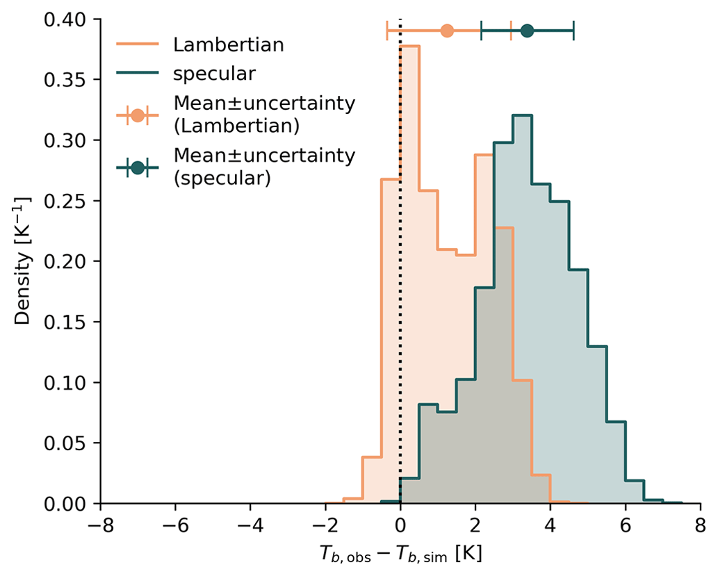
Figure 2 Histogram and mean of the difference between observed and simulated 183.31±5 GHz TBs (T_b,obs and T_b,sim, respectively), employing 183.31±7.5 GHz emissivities under Lambertian and specular surface reflection during the AFLUX campaign. The TB bin width is 0.5 K.

4 Airborne observations

4.1 Case study

In this section, we first illustrate the available airborne observations collected along an 11 km transect during AFLUX RF08 on 31 March 2019 (Fig. 3). Satellite observations indicate that ∼75 % of the ice within the area is multiyear ice (Fig. A1). The sea ice types along the transect are distinguishable in airborne visual-camera observations (Fig. 3a–d) and Sentinel-2B imagery (Fig. 3e). We observe predominantly snow-covered sea ice from 0 to 7 km. Notably, surface structural variations from 3 to 4 km suggest the presence of young ice, defined as the transition stage between nilas and first-year ice (World Meteorological Organization, 2014) that is sometimes formed within leads among thicker multiyear ice. Progressing from 7 to 11 km, we encounter refrozen leads with nilas attached to individual snow-covered ice floes. The observed surface temperatures reflect the changing sea ice and snow properties, with almost constant temperatures of −24 °C over snow-covered sea ice and up to −18 °C over nilas. The TBs vary significantly with ranges of 76, 47, 48, and 30 K at 89, 183.31±7.5, 243, and 340 GHz, respectively, and exceed the 6 K surface temperature range. This high variability demonstrates the importance of surface emissivity variations in the observed TB.

The difference between the minimum and maximum sea ice emissivity decreases as frequency increases, with values of 0.35, 0.27, 0.24, and 0.21 at 89, 183.31±7.5, 243, and 340 GHz, respectively. The higher emissivity variability at 89 GHz compared to the other frequencies likely relates to its horizontal polarization at a 25° incidence angle. Previous studies have shown that horizontal polarization exhibits higher sea ice emissivity variability at 89 GHz than vertical polarization does at an incidence angle of 53° (e.g., Shokr et al., 2009). This is related to the enhanced sensitivity to sea ice and snow properties with horizontal polarization. Similar effects likely occur at a 25° incidence angle. Furthermore, horizontal polarization at 89 GHz results in emissivities that are up to 0.05 lower compared to nadir, depending on the sea ice type, as shown in past airborne observations at varying incidence angles (Hewison and English, 1999). This partly explains the low emissivity at 89 GHz observed here compared to that from the other nadir-viewing channels.

Despite the implications of incidence angle and polarization differences on spectral features, this transect showcases typical sea ice emission signatures. Over nilas from 7 to 11 km, sea ice emissivity increases across all channels, with values ranging from 0.9 to 1. Hewison and English (1999) and Hewison et al. (2002) observed similar emissivities at 89 and 183 GHz over bare ice under the same observing geometry as MiRAC. Sea ice emissivity over multiyear ice within the first 7 km is lower than that over nilas at all frequencies. The snow-covered and refrozen leads from 3 to 4 km only cause higher emissivities at 89 GHz, likely due to the higher sensitivity of the horizontal polarization at this channel to sea ice and snow properties. Observations of multiyear ice at nadir in Hewison et al. (2002) are comparable to multiyear ice observations along this transect. The 243 GHz nadir emissivity is close to the mean emissivity of 0.84 at 220 GHz, observed by Haggerty and Curry (2001). The alignment of MiRAC emissivity features with past sea ice emissivity studies provides confidence in the 243 GHz emissivity resolved at the hectometer scale. Moreover, the high similarity between 243 and 340 GHz emissivities shows that MiRAC provides submillimeter sea ice emissivities with a clear dependence on distinct sea ice types for the first time.

The ±8 K surface temperature uncertainty causes the highest emissivity uncertainty for all channels (not shown). The uncertainty magnitude varies highly between the channels. The lowest uncertainty range occurs at 89 and 243 GHz, while the highest range occurs at 183.31±2.5 GHz, which is the channel closest to the 183.31 GHz water vapor absorption line, exceeding the 40 K surface sensitivity threshold. In the following, we only show the 183.31±7.5 GHz channel due to its higher surface sensitivity and similar emissivity compared to the inner 183 GHz channels (Fig. 3j). The measured emissivity difference between multiyear ice and nilas exceeds the emissivity uncertainty at all frequencies, while no significant variations occur in the first 7 km at 340 GHz. Overall, this case study demonstrates the relevance of sensitivity tests in interpreting the retrieved emissivities to distinguish emissivity features arising from uncertainties inherent to the assumptions of the emissivity calculation, caused by unknown subsurface temperatures and uncertain atmospheric thermodynamic profiles.

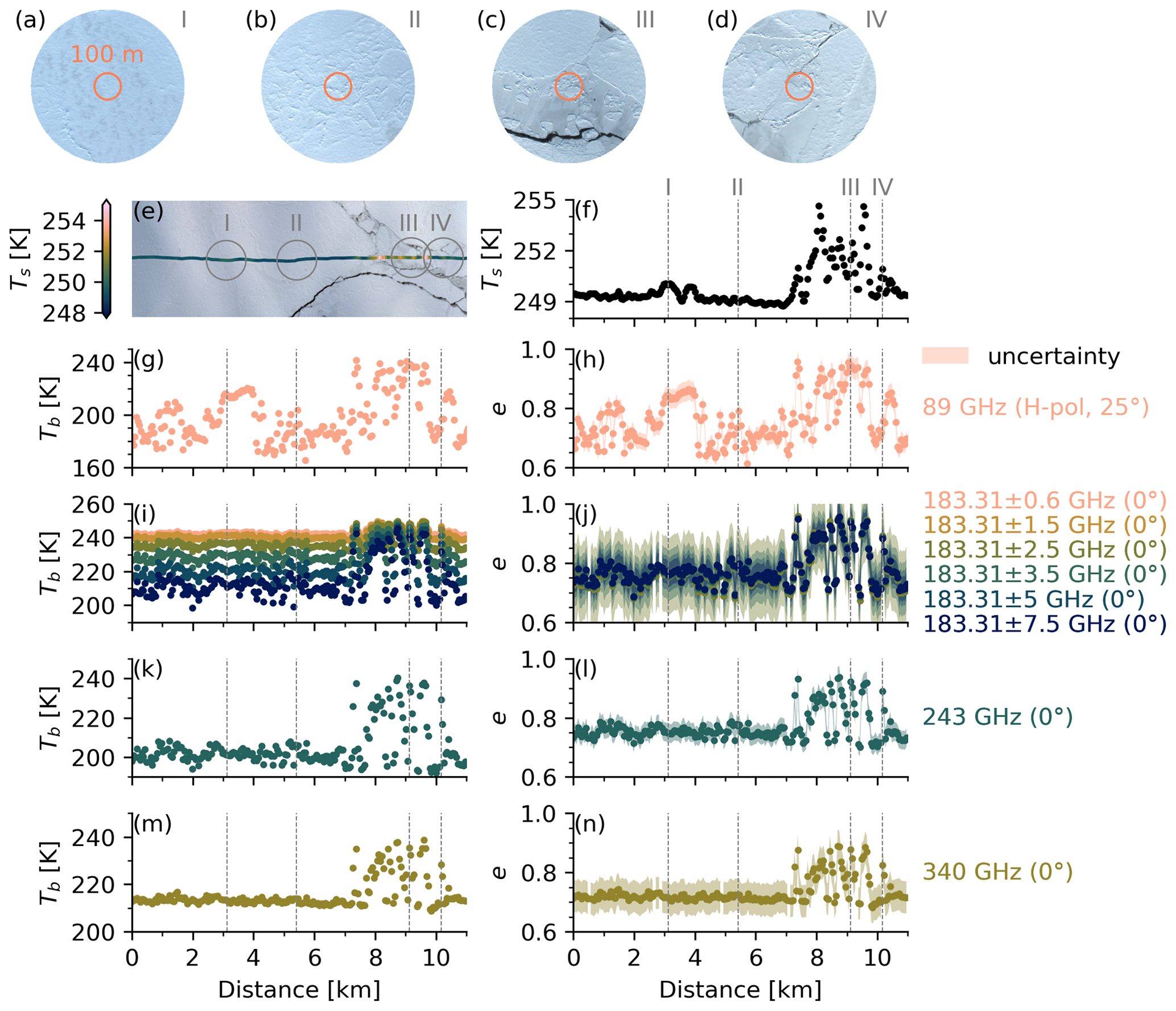
Figure 3 Observations collected along an 11 km transect at 81.01° N, 4.28–4.91° E (about 100 km north of the sea ice edge) during AFLUX RF08 (31 March 2019). Polar 5 flew westward (right to left in this figure) at an altitude of 540 m for about 4 min, starting at 11:39 UTC. (a–d) Fish-eye lens images with a 100 m diameter nadir reference circle obtained at (a) 11:42:16 UTC, (b) 11:41:32 UTC, (c) 11:40:20 UTC, and (d) 11:40:00 UTC. (e) Sentinel-2B L2A natural-color image obtained at 14:37 UTC, showing the flight track, surface skin temperature from the KT-19, and the location of the airborne imagery. (f) Surface skin temperature from the KT-19. (g, i, k, m) TB at all MiRAC channels. (h, j, l, n) Emissivity and uncertainty from MiRAC's surface-sensitive channels, i.e., except the two inner 183 GHz channels in this case. The Sentinel-2B image was shifted northward by 2.5 km to correct for sea ice drift. H-pol: horizontal polarization

4.2 TB and emissivity variability

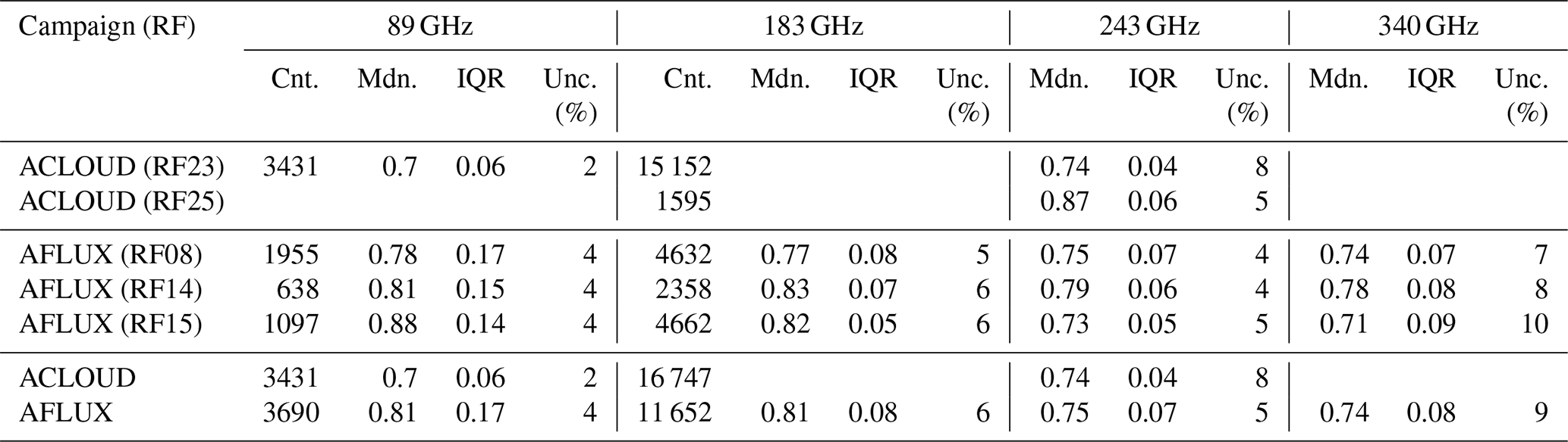
In the following, we analyze the distributions of TB and emissivity observed during all clear-sky flights over sea ice during the ACLOUD and AFLUX campaigns (Fig. 4). The histograms corresponding to 89 GHz and 183–340 GHz include different samples due to the exclusion of low flight altitudes at 89 GHz, which introduces a potential inconsistency (Table 3). Therefore, we compared these histograms with those from instantaneous measurements in which all channels sample the same sea ice, and we found no changes in the shape of the histograms that exceed the estimated emissivity uncertainties (not shown). Hence, we present all available observations here. The TB variability during the AFLUX campaign exceeds that during the ACLOUD campaign at all frequencies (Fig. 4a–d). The ACLOUD TBs at 183, 243, and 340 GHz show low variability and higher values, attributed to the increased atmospheric water vapor and surface temperature. Two distinct peaks occur at 89 and 243 GHz during the AFLUX campaign. These peaks become even more pronounced in the emissivity distributions, ranging from around 0.7 to 0.85 and from 0.9 to 1, respectively (Fig. 4e–h). These emissivity ranges correspond to those pertaining to multiyear ice and nilas in the AFLUX RF08 case (see Sect. 4.1). The histograms derived for 243 GHz are broader than the 220 GHz emissivities reported by Haggerty and Curry (2001) due to MiRAC's higher resolution, which captures previously unresolved leads. MiRAC's 340 GHz emissivity distribution follows a similar shape to the 183 and 243 GHz channels. The broader emissivity distribution at 340 GHz could be related to the higher emissivity uncertainty of 9 % compared to the emissivity uncertainty at 183 GHz (6 %) and 243 GHz (5 %) during the AFLUX campaign (Table 3). The apparent shape difference of the 89 GHz distribution and the 2-fold higher interquartile range (Table 3) indicate that this horizontally polarized and 25° inclined channel is more sensitive to sea ice and snow properties than the other channels at higher frequencies. The 89 GHz distribution is narrower during the ACLOUD campaign than during the AFLUX campaign in the presence of melting sea ice, which agrees with findings from Haggerty and Curry (2001). Lower emissivities during the ACLOUD campaign, indicated by the two lower peaks around 0.65, correspond to regions with lower sea ice concentrations. These emissivities should be treated with care due to the specular contributions of the sea surface.

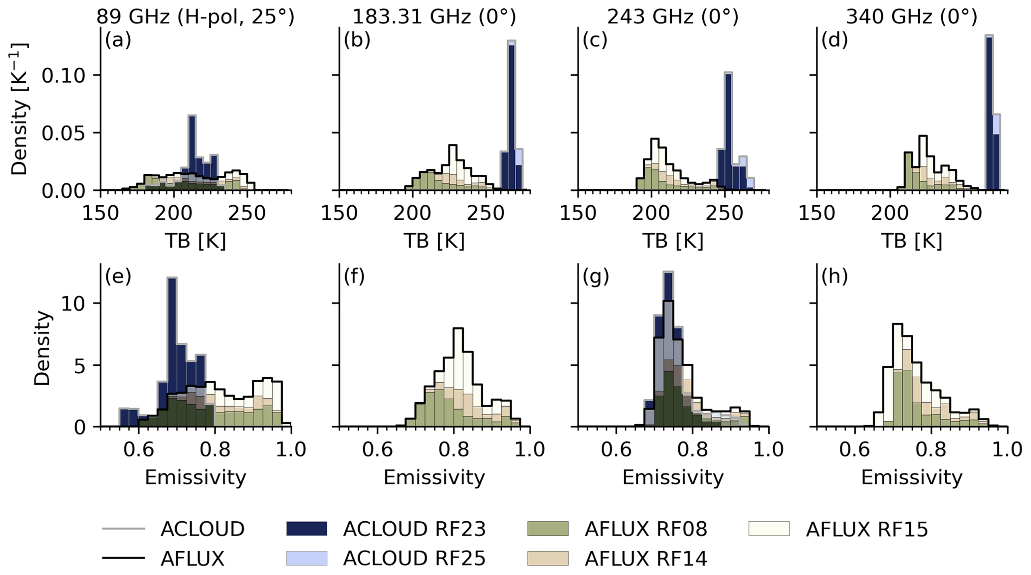
Figure 4 Histograms of (a–d) TB and (e–h) emissivity at (a, e) 89, (b, f) 183, (c, g) 243, and (d, h) 340 GHz during the ACLOUD and AFLUX campaigns. The TB bin width is 5 K, and the emissivity bin width is 0.025. The observations at 183 and 340 GHz collected during the ACLOUD campaign fall below the surface sensitivity threshold and are therefore excluded from panels (f) and (h). The histograms for 183, 243, and 340 GHz contain more samples than the 89 GHz histogram (see Table 3).

Table 3 Sea ice emissivity at MiRAC frequencies during individual flights and across all flights from the ACLOUD and AFLUX campaigns. Values include the sample count (Cnt.), median (Mdn.), interquartile range (IQR), and relative uncertainty averaged over all samples (Unc.). The sample counts for 183, 243, and 340 GHz are constant, except for the ACLOUD flights, where emissivities measured at 183 and 340 GHz are not available.

4.3 Influence of sea ice and snow properties

In this section, we aim to relate the observed sea ice emissivity variability to sea ice and snow properties visible in fish-eye lens images and surface skin temperature. Previous airborne studies have classified sea ice based on airborne imagery or visual inspection and calculated emissivity spectra for each sea ice type (e.g., Hewison and English, 1999). However, this approach requires sea ice classification at a high temporal resolution. Therefore, we use k-means clustering to extract distinct emissivity spectra – a similar approach to that seen in previous sea ice and snow emissivity studies (Wang et al., 2017b; Wivell et al., 2023). First, we normalize the data by subtracting the mean emissivity and dividing the result by the standard deviation at each channel to ensure equal channel weighting. Then, we cluster the normalized emissivity spectra across all four MiRAC frequencies using k-means to identify distinct sea ice emissivity spectra.

The crucial hyperparameter for k-means clustering is the total number of clusters. Therefore, we analyze three heuristics – distortion (Thorndike, 1953), the Calinski–Harabasz index (Calinski and Harabasz, 1974), and silhouette score (Rousseeuw, 1987) – and yield an optimal cluster number of four (Appendix B). However, not all clusters separate clearly due to transitional stages and inhomogeneous sea ice properties within MiRAC's footprint (Fig. B1b). Fish-eye images for all samples underline the high diversity in sea ice and snow properties (Fig. B2).

The occurrence of each cluster varies between the flights. Cluster 1 (C1) occurs more often than the other clusters (appearing in 52 % of cases during RF08), while C2 is predominant during RF14 (accounting for 68 % of occurrences), and C3 is observed in 48 % of instances during RF15. C4 occurs about 20 % of the time during RF08 and RF14, and it occurs 8 % of the time during RF15. It is unclear whether these changes are due to sea ice drift or temporal changes in ice properties, given the coarse temporal resolution and potential bias resulting from the flight pattern.

Each cluster exhibits distinct emissivity features (Figs. 5a and C1). The lowest emissivity prevails in C1, and the highest is found in C4. C1 occurs over snow-covered sea ice (Fig. 5c), which might be classified as multiyear ice and predominates during the AFLUX flights (Fig. A1). This also corresponds to the lower skin temperature of 250 K for this cluster compared to the other clusters (Fig. 5b). Few open leads are present within C1 as water shows a spectral signature similar to that of this cluster. C4 occurs over nilas in refrozen leads (Fig. 5c). This aligns with the generally warmer skin temperature observed in this cluster compared to in the other clusters (Fig. 5b). C4 is distinct from the other three clusters at 183, 243, and 340 GHz. C2 emissivities fall between those of C1 and C4 at all frequencies. This cluster occurs over various surface types, but it predominantly occurs over ice with visual properties of first-year ice. C3 emissivities are close to those of C4 at 89 GHz and close to those of C1 at 243 and 340 GHz. This cluster occurs over young ice that has more snow cover than the sea ice in C4. Hence, scattering within the upper snow layer could explain the lower emissivity at 243 and 340 GHz in C3 than in C4. However, the emissivity is lower than in C2, where snow is also present, which indicates the importance of other factors, such as snow density and grain size.

The evaluation of airborne emissivities reveals (1) low differences in the median emissivity and interquartile range at 183, 243, and 340 GHz; (2) higher emissivities over nilas compared to those over multiyear ice at all frequencies; and (3) four distinct emissivity spectra. The similarity between 243 and 340 GHz implies a lower spectral variation in sea ice emissivity in the submillimeter wave range. However, the emissivity variability at both frequencies is still notable and depends on the sea ice type, with the highest contrast observed between multiyear ice and nilas.

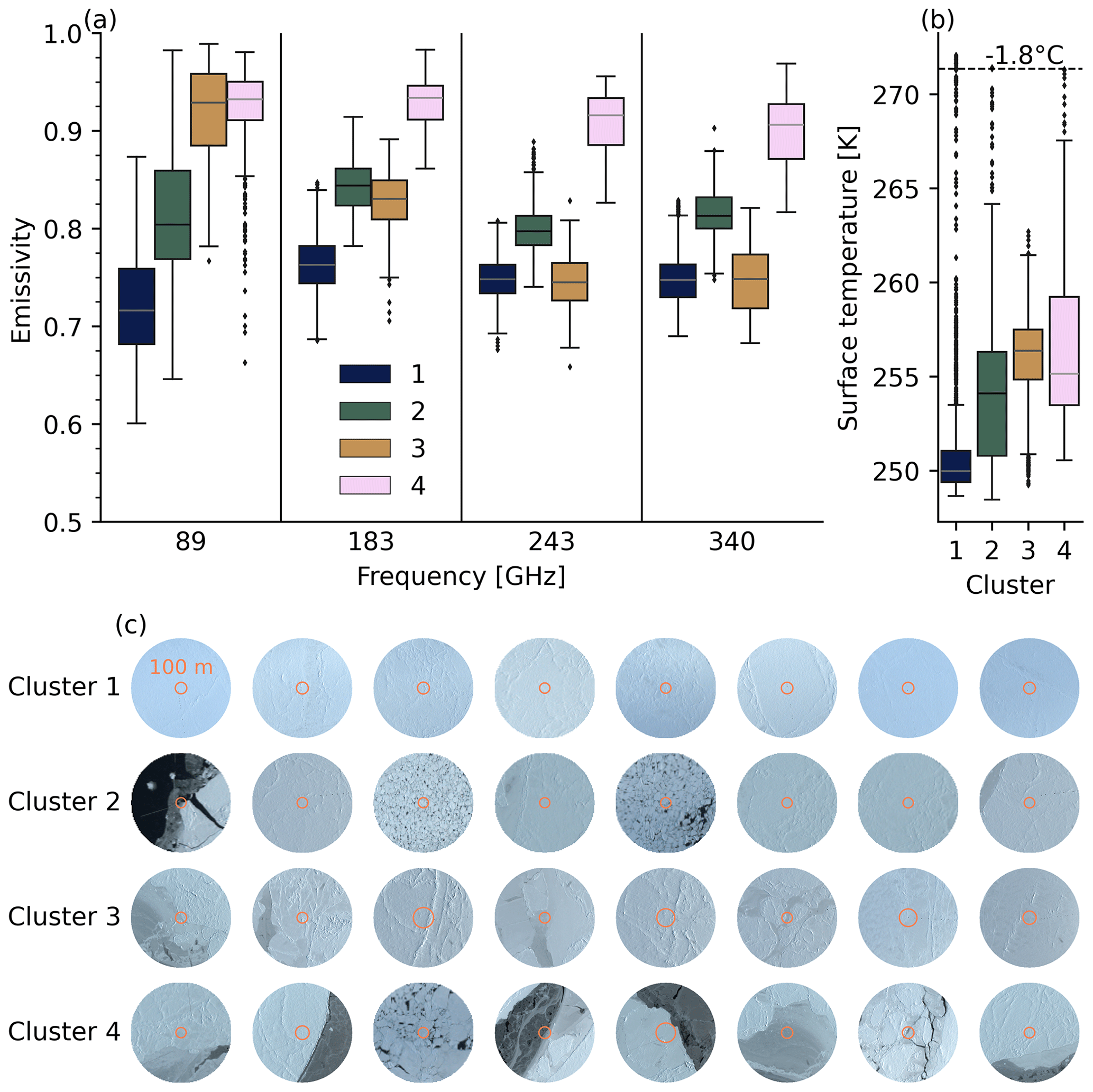
Figure 5 Comparison of sea ice emissivity and surface temperature across k-means clusters. (a) Tukey boxplot depicting the distribution of sea ice emissivity at MiRAC frequencies within each k-means cluster. (b) Tukey boxplot showing the distribution of surface temperature within each k-means cluster. (c) Fish-eye lens images representing the k-means cluster centroids, i.e., for emissivity samples similar to the mean cluster emissivity, with a 100 m diameter nadir reference circle (see Fig. B2 for all images). It should be noted that the actual footprint might not lie within the indicated region due to the aircraft attitude causing MiRAC-P to point off-nadir by a few degrees and potential temporal shifts between the camera and MiRAC.

5 Comparison with satellites

5.1 Spatial variability at a subfootprint scale

Airborne and satellite observations resolve sea ice emissivity on different spatial scales. Hectometer-scale airborne observations resolve most leads, while kilometer-scale satellite observations partially smooth out these structures. Figure 6a shows a Polar 5 transect during AFLUX RF08, covering a 5 km lead mainly composed of nilas. MiRAC's 89 GHz emissivity exhibits a pronounced increase from multiyear or first-year ice to nilas, followed by a sharp decrease over a short section of open water. Consequently, emissivity clusters shift from C1 over multiyear or first-year ice to C4 over younger sea ice. The 5 km AMSR2 footprints partially resolve the lead, with higher emissivities observed over nilas, whereas the 16×16 km² MHS footprints cannot fully capture it. This example underscores the significance of subfootprint-scale emissivity variations over spatially heterogeneous sea ice.

Next, we examine how emissivity varies with footprint size from 0.1 to 20 km for all airborne observations. We calculate the larger-scale emissivity from the mean airborne surface temperature and emission for each footprint size interval. The interquartile range of the emissivity decreases rapidly with increasing footprint size during the ACLOUD and AFLUX campaigns at all frequencies (Fig. 6b). For example, the variability in 100 m footprints at 340 GHz during the AFLUX campaign decreases by 42 % (65 %) when the footprint size corresponds to 5×5 km² (16×16 km²). The smallest decrease occurs at 89 GHz during the ACLOUD campaign, with a decrease of 21 % (20 %) when the footprint size reaches 5×5 km² (16×16 km²). Hence, a larger satellite footprint averages out small-scale emissivity variations.

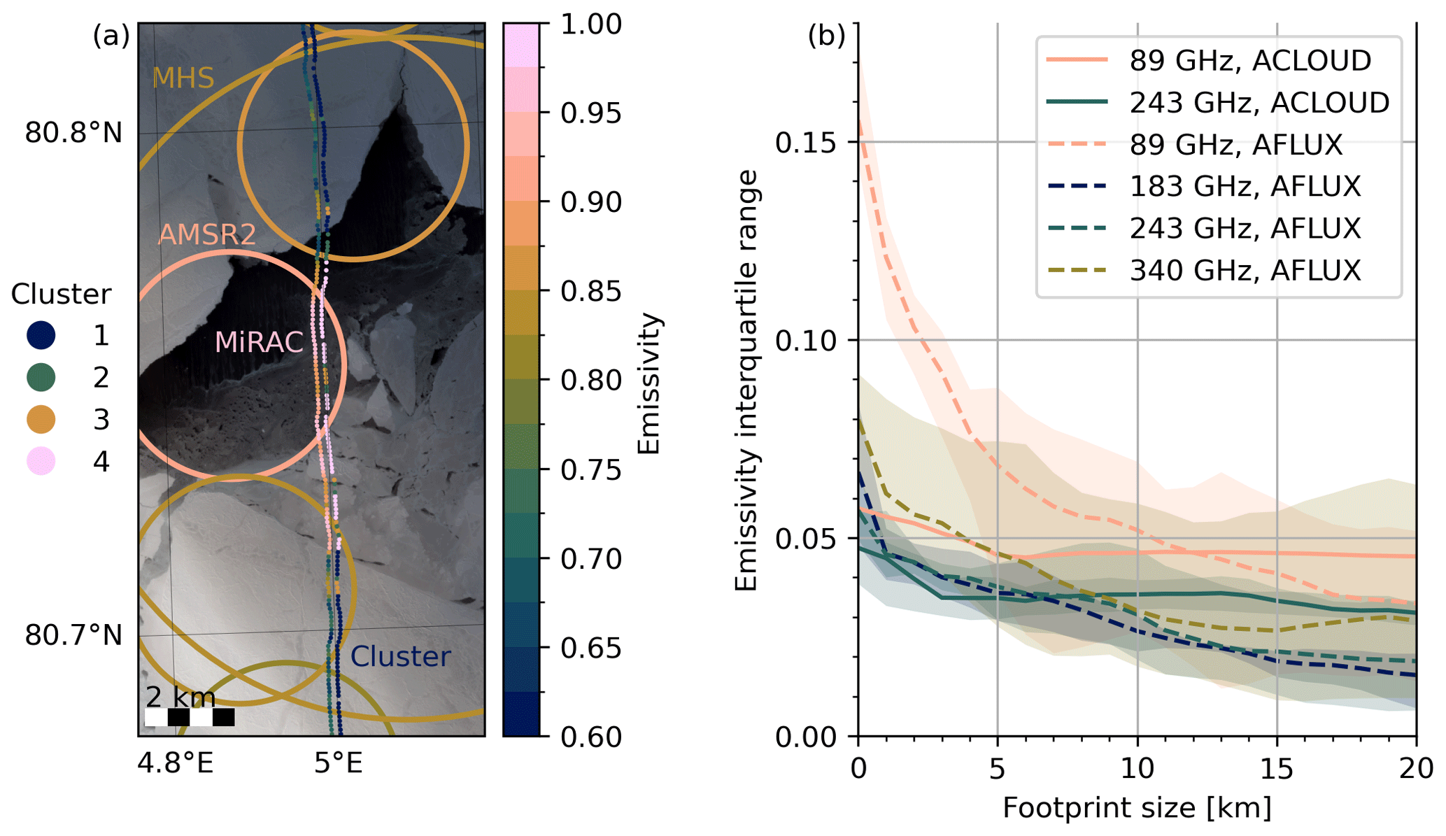
Figure 6 (a) Sea ice emissivity at 89 GHz from MiRAC (10:32 to 10:37 UTC), AMSR2 (11:02 UTC), and MHS onboard Metop-B (11:38 UTC) during AFLUX RF08 on 31 March 2019. The MiRAC emissivity cluster is displayed 100 m east of the emissivity. The actual MiRAC footprints lie between the emissivity and emissivity cluster locations. The background shows a Sentinel-2B L2A natural-color image that was obtained at 14:37 UTC and shifted 4 km northward to correct for sea ice drift. (b) The emissivity interquartile range as a function of footprint size from 0.1 to 20 km for all flights and channels. The spread represents the minimum and maximum interquartile ranges for each campaign.

5.2 Channel intercomparison

Before integrating MiRAC data with all satellite observations to study spectral variations of up to 340 GHz on a satellite scale, we must ensure that our collocation approach reproduces satellite observations at similar frequencies and observing geometries. The near-nadir (0–30°) 157 GHz MHS and 165.5 GHz ATMS channels are comparable to MiRAC's 183 GHz channel at nadir. We compare these satellite channels rather than the 190.31 and 183.31±7 GHz channels due to their higher surface sensitivity and lower uncertainty, even though spectral emissivity gradients might occur (e.g., Hewison et al., 2002). Other channel or instrument combinations differ in terms of incidence angle or polarization, making footprint-level comparisons less meaningful.

Figure 7 illustrates the resampling process, which transitions from MiRAC's high-resolution emissivity to the satellite footprints. It also shows the corresponding satellite emissivity and the differences for all AFLUX flights. Notably, MiRAC reveals hectometer-scale emissivity features, such as leads, which are not captured by MHS and ATMS due to their 16×16 km² footprint. This high hectometer-scale variability consistently occurs within each satellite footprint (right column in Fig. 7) and diminishes after resampling to the satellite footprint scale. The limited spatial coverage of MiRAC causes deviations from MHS and ATMS as MiRAC only captures a narrow strip of the satellite footprint (e.g., during AFLUX RF08 near 80.4° N, 5° E; Fig. 7a), resulting in the highest emissivity bias (Fig. 7d). However, the collocation method is robust in most cases and yields MiRAC emissivities that are representative of the 16×16 km² satellite footprints. Moreover, the assessment of relative bias, calculated by subtracting the MiRAC emissivity from MHS or ATMS emissivity and dividing the result by the MiRAC emissivity, yields insights into the consistency of MiRAC observations from satellites (Tables 4 and 5). This relative bias of −3 % to 1 % falls well within MiRAC's 6 % uncertainty range at 183 GHz (see Table 3). The correlation between MiRAC and MHS or ATMS ranges from 0.4 to 0.6 and reflects the partial footprint overlap, reducing the representation of MiRAC for each satellite footprint. In summary, the comparison with MHS and ATMS provides confidence in the accuracy of our airborne-emissivity estimates and the reliability of converting from hectometer to satellite footprint scales. Hence, we can apply the same approach to other MiRAC channels at frequencies up to 340 GHz.

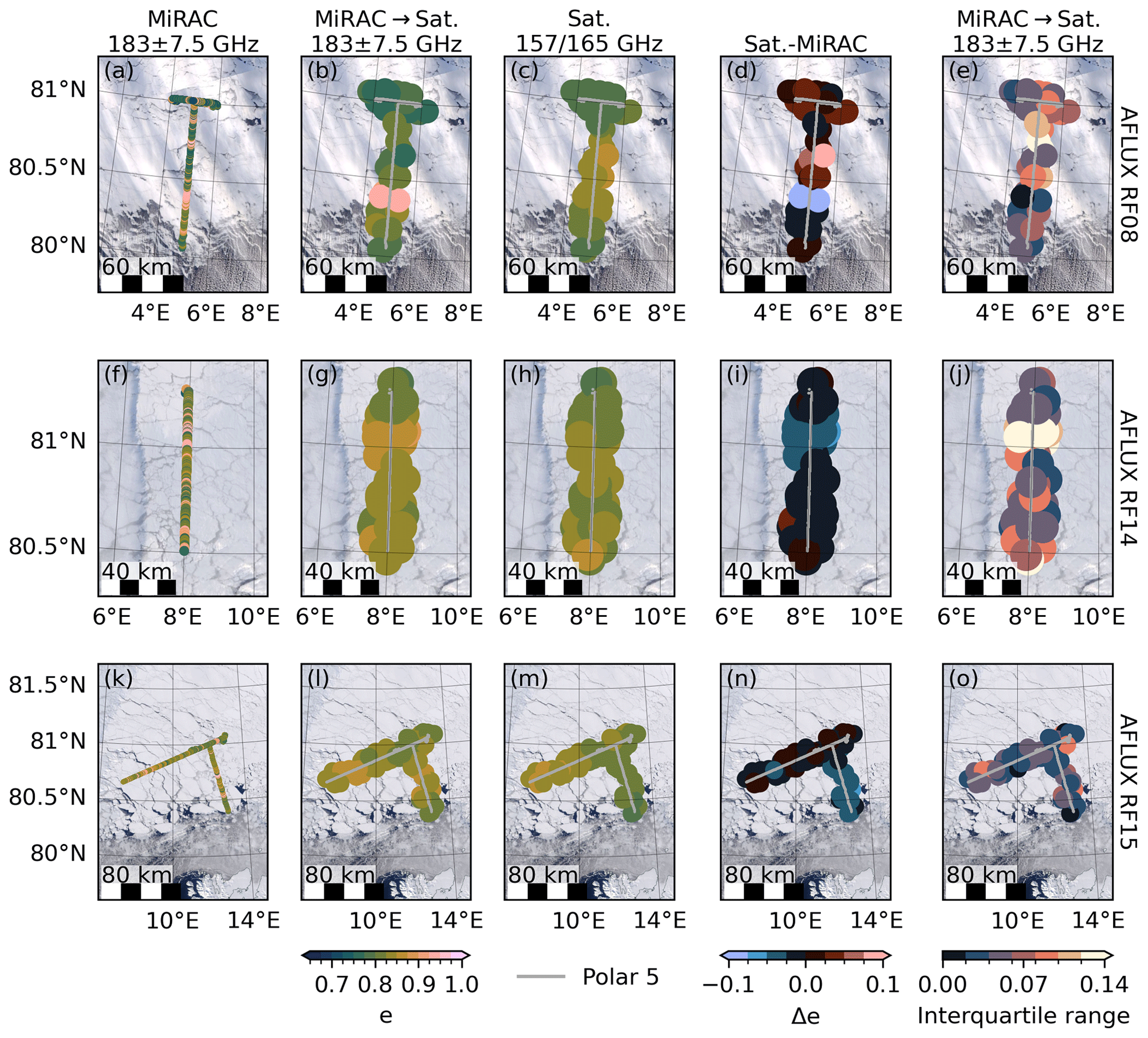
Figure 7 Comparison of emissivity from nadir 183 GHz MiRAC observations and near-nadir (0–30°) 157 GHz MHS and 165.5 GHz ATMS observations collected along the Polar 5 flight track during AFLUX RF08, RF14, and RF15 (rows). (a, f, k) MiRAC emissivity at the original resolution. (b, g, l) MiRAC emissivity resampled to satellite (Sat.) footprints. (c, h, m) Satellite emissivity. (d, i, n) Emissivity difference between MiRAC and the satellites (satellite emissivity minus MiRAC emissivity). (e, j, o) MiRAC emissivity interquartile range within the satellite footprint. No 183 GHz observations from MiRAC were available during the ACLOUD campaign. The background images are composites of MODIS onboard Terra from the same day (NASA Worldview). All footprints are approximated as circles. MiRAC's footprints are enlarged to a 5 km diameter. The satellite footprint size corresponds to the footprint size at nadir.

Table 4 Comparison of collocated emissivity from nadir 183 GHz MiRAC observations and near-nadir (0–30°) 157 GHz MHS observations collected during the three AFLUX flights. Values include the number of collocated satellite footprints (Count); median; interquartile range (IQR); relative bias (Rel. bias), i.e., MHS emissivity minus MiRAC emissivity divided by MiRAC emissivity; relative root-mean-square deviation (Rel. RMSD), normalized by MiRAC emissivity; and Pearson's correlation coefficient (Corr.).

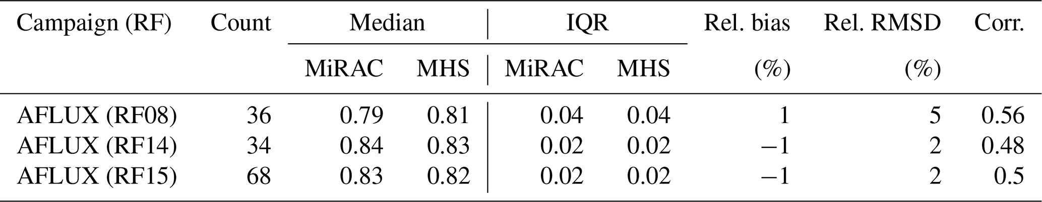
Table 5 Comparison of collocated emissivity from nadir 183 GHz MiRAC observations and near-nadir (0–30°) 165.5 GHz ATMS observations collected during the three AFLUX flights. The columns are identical to those in Table 4.

5.3 Spectral variations

In this section, we collocate MiRAC with MHS, ATMS, SSMIS, and AMSR2 to analyze spectral variations in sea ice emissivity from 88 to 340 GHz as well as angular and polarization effects. We group all collocated emissivities by frequency into the following categories: 88–92, 150–165 (only for satellites), 176–190, 243, and 340 GHz. The MiRAC observations are averaged to align with the collocated footprints of each satellite instrument, ensuring equivalent spatial sampling (see Sect. 2.5).

The channel-dependent emissivity variability observed on a satellite scale during the ACLOUD and AFLUX campaigns reveals distinct features related to spectral, angular, and polarization differences (Fig. 8). Low spectral differences during the ACLOUD campaign occur near nadir from 89 to 243 GHz (MHS and MiRAC) and at vertical polarization from 91 to 150 GHz (SSMIS; Fig. 8a). The higher satellite emissivity can be attributed to the underestimation of the NE23 skin temperature compared to that of the KT-19. As expected, the 89 GHz emissivity shows a polarization signal of about 0.1. This indicates a specular contribution to surface reflection and an underestimation of emissivity in the case of purely Lambertian reflection at 89 GHz for MiRAC (see Sect. 3.3). Combining both polarizations from SSMIS or AMSR2 with quasi-vertical polarization, following Eq. (1), reduces the absolute emissivity difference, meaning it falls within the 0–30° emissivity range of MHS. Furthermore, the horizontally polarized 89 GHz channel of MiRAC is closer to the horizontally polarized channels of SSMIS and AMSR2. Spectral differences observed during the AFLUX campaign exceed those observed during the ACLOUD campaign, which might be due to contrasting sea ice properties (i.e., melting conditions during the ACLOUD campaign versus much colder and dryer sea ice and snow during the AFLUX campaign; Fig. 8b). The near-nadir emissivity remains constant from 89 to 183 GHz but decreases near frequencies of 243 and 340 GHz. No significant difference in spectral emissivity can be detected in the 165 to 183 GHz frequency range, where all satellites fall within MiRAC's 6 % uncertainty (see Table 3)). The decrease around 243 GHz exceeds the 243 GHz emissivity uncertainty. The AFLUX emissivities show a lower polarization difference at 89 GHz compared to the ACLOUD emissivities, which can be attributed to the lower amount of open water between ice floes during the AFLUX campaign. The emissivity of the 89 GHz MiRAC channel lies between the horizontally polarized AMSR2 and SSMIS channels and the near-nadir MHS and ATMS channels.

Different instruments show similar emissivity distributions at similar channels. For example, the three MHS and ATMS channels exhibit nearly identical distributions during the AFLUX campaign (see Fig. 8b). Additionally, the polarized 89 GHz channels of the SSMIS and AMSR2 show good agreement. However, during the ACLOUD campaign, emissivity differences between AMSR2 and SSMIS are noted for the vertically polarized channel, primarily due to the low number of collocated AMSR2 footprints compared to MiRAC footprints. For the AFLUX campaign, where the footprint counts of SSMIS and AMSR2 are comparable, AMSR2 shows higher variability as it has a smaller footprint than SSMIS.

Furthermore, MiRAC distributions align with MHS and ATMS distributions near nadir. The increased emissivity variability in MiRAC's 25° inclined 89 GHz channel, compared to that of MHS and ATMS, may be explained by its horizontal polarization. When comparing the vertically and horizontally polarized SSMIS and AMSR2 channels, horizontal polarization exhibits higher variability, consistent with findings from experiments by Shokr et al. (2009).

The consistent outcomes from spaceborne and airborne observations unveil a first-time representation of sea ice emissivity variability from 89 to 340 GHz. As detected by MiRAC, hectometer-scale emissivity variations smooth out when observed from a satellite perspective. Our analysis shows a potential decline in emissivity from 183 to 243 GHz under cold and dry conditions during the AFLUX campaign. This spectral pattern occurs within airborne emissivity clusters – i.e., within C3 (young ice) and, to some extent, within C2 (first-year ice) and C4 (nilas) – but is notably absent in C1 (multiyear ice) and prevails after being resampled onto a satellite scale. These cluster differences underscore the importance of spatial distributions among sea ice types.

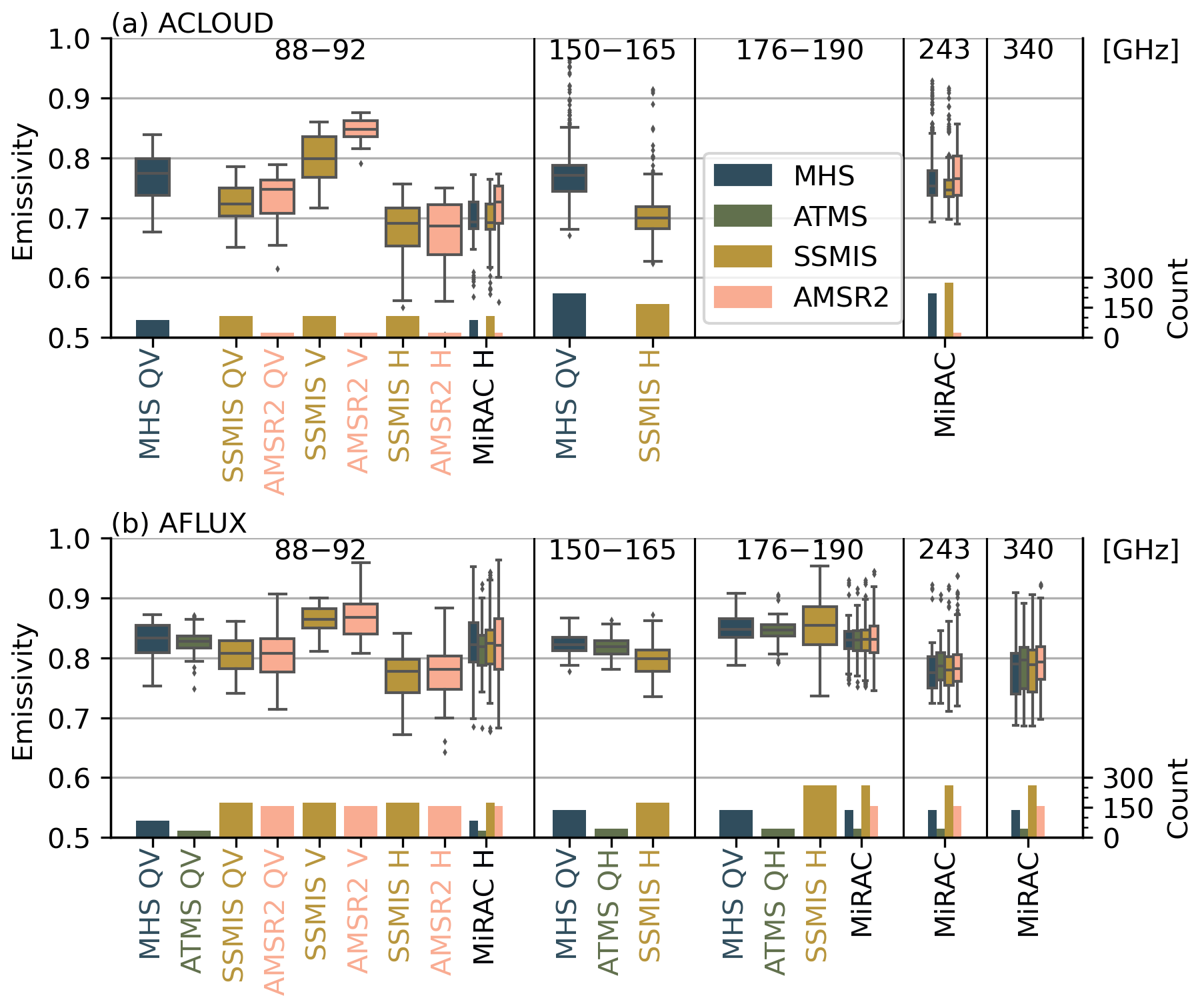
Figure 8 Tukey boxplots of collocated emissivity observed during (a) the ACLOUD campaign and (b) the AFLUX campaign for the frequency ranges 88–92, 150–165, 176–190, 243, and 340 GHz, derived from MHS (0 to 30°), ATMS (0 to 30°), SSMIS (53°), AMSR2 (55°), and MiRAC (25° at 89 GHz and 0° at 183, 243, and 340 GHz). The secondary axis denotes the count of the collocated footprints. Quasi-vertical SSMIS QV and AMSR2 QV polarizations are characterized by dominant contributions of 64 % and 67 %, respectively, from horizontal polarization. The 88–92 GHz satellite footprint count might be lower than the satellite footprint count at frequencies above 150 GHz because satellite footprints are excluded if the nearest MiRAC channel exhibits no emissivity. Note that no ATMS overpass occurred during the ACLOUD campaign.

6 Conclusions

The upcoming launches of ICI and EPS–Sterna, featuring novel frequencies above 200 GHz, and AMSR3, exhibiting a novel AMSR2-like resolution at 183 GHz, require an improved understanding of sea ice emissivity to distinguish atmospheric and surface microwave signals under dry polar conditions (Wang et al., 2017b). However, few field observations have measured sea ice emissivity at such high frequencies using a hectometer-scale resolution. Therefore, we analyzed sea ice emissivity variations observed with the MiRAC microwave radiometer during two airborne field campaigns – the ACLOUD campaign (summer 2017) and the AFLUX campaign (spring 2019). The flights analyzed in this study covered about 1700 km of distance. Moreover, 7000 samples were collected at 89 GHz (25° incidence angle; horizontal polarization), 28 000 samples were collected at 243 GHz (nadir), and 11 000 samples were collected at 183 and 340 GHz (nadir).

Our first objective was to identify critical physical sea ice and snow properties affecting emissivity up to submillimeter wavelengths. Sea ice emissivity exhibits high variability, ranging from about 0.65 to 1, with the lowest emissivities observed at 89 GHz. The 89 GHz distribution showed higher variability than the nadir channels due to its inclination and horizontal polarization. MiRAC resolves sea ice emissivity features that align with sea ice and snow properties identified from visual imagery. Four emissivity spectra from 89 to 340 GHz could be identified through k-means clustering. These spectra predominantly correspond to multiyear ice, first-year ice, young ice, and nilas. However, the emissivity variability for each cluster is significant due to variations in snow or sea ice microphysical properties and mixed types within the radiometer footprint. The lowest emissivity is observed over multiyear ice, and the highest emissivity is found over nilas, consistent with previous studies conducted at 89 and 183 GHz (NORSEX Group, 1983; Hewison and English, 1999; Hewison et al., 2002).

Our second objective was to relate the observed hectometer-scale emissivity observations to the satellite scale. We collocated MiRAC with MHS, ATMS, SSMIS, and AMSR2 for this purpose. Satellite instruments do not resolve hectometer-scale sea ice emissivity variations observed by MiRAC due to their larger footprints. By averaging the airborne observations, we estimated the decrease in the emissivity interquartile range as footprint size increases. The reduction in the interquartile range is most significant during the AFLUX campaign, when leads induce significant hectometer-scale emissivity variations. For example, the emissivity interquartile range decreases by almost half from the hectometer scale to a footprint of 16×16 km², typical of microwave satellite instruments. We find high agreement between MHS, ATMS, and MiRAC emissivities near 183 GHz. During the AFLUX campaign, emissivity decreases significantly from 183 to 243 GHz, while it remains almost constant during the ACLOUD campaign. The estimates provided here may represent the emissivities that future satellites, such as ICI and EPS–Sterna, will observe.

The study's implications are as follows:

• The first implication involves hectometer-scale frequency dependency. The 183, 243, and 340 GHz channels exhibit similar hectometer-scale sea ice emissivity variations at nadir, regardless of the sea ice type (e.g., multiyear ice and nilas). This finding is crucial for the development of airborne retrieval methods.

• The second concerns spatial and temporal representation. At the satellite footprint scale, hectometer-scale sea ice emissivity variations average out, which facilitates sea ice emissivity parameterization. However, these variations become more relevant for higher-resolution channels, such as AMSR2.

• The third pertains to emissivity frequency extrapolation. The relatively low spectral variation in emissivity at the satellite scale from 89 to 340 GHz at nadir supports using a first-order approximation of constant emissivities over sea ice within existing parameterizations, such as TELSEM2 (Wang et al., 2017b). Accounting for spatial and temporal emissivity variations appears to be more relevant than focusing on spectral gradients.

This study has several limitations:

• The first limitation concerns channel intercomparison. The 25° inclination and horizontal polarization of the 89 GHz channel may affect comparisons with the 183–340 GHz nadir-viewing channels by increasing the channel's variability and lowering its emissivity compared to an 89 GHz nadir-viewing channel. Quantification of this effect might be possible by analyzing the airborne HALO–(AC)³ campaign conducted in spring 2022 (Wendisch et al., 2021).

• Another limitation involves surface temperature assumption. Using the surface skin temperature rather than the emitting-layer temperature imposes a frequency-dependent bias on emissivity measurements collected during the AFLUX campaign.

• Sea ice and snow properties pose another limitation. The aerial images provide only a broad perspective on sea ice and snow properties and have limitations in providing vertical profiles of sea ice microphysics, such as density, grain size, or salinity.

• Spatial resolution is also a limiting factor. MiRAC's hectometer scale may not resolve smaller sea ice features, such as ridges or melt ponds, which could influence emissivity.

• There are also spatial and temporal limitations. Field observations are limited in space (approximately 100 km) and time (5 d), potentially restricting the generalizability of findings across polar regions.

Three primary challenges persist when it comes to comprehending sea ice emissivity variations to advance atmospheric and surface retrievals over sea ice. First, the relatively unexplored emissivity dependence on polarization and incidence angles, especially at frequencies above 200 GHz, demands comprehensive investigation. Potential solutions include utilizing shipborne or airborne observations with scanning radiometers. Second, the high uncertainty due to atmospheric emissions that mask spectral features of emissivity, particularly at 340 GHz and over the more reflective multiyear ice, requires simultaneous measurements of near-surface downwelling atmospheric TB for emissivity calculations. Third, observed emissivity spectra must be combined with in situ measurements of sea ice and snow microphysics to advance radiative-transfer modeling. In summary, addressing these challenges will help bridge remaining knowledge gaps in sea ice microwave emissivity and will have implications for current and upcoming satellite missions. Future work will need to focus on separating sea ice and atmospheric signals under all-sky conditions.

Appendix A: Multiyear ice concentration maps

We include maps illustrating multiyear ice concentration to offer additional context for the three AFLUX flights (Fig. A1). The multiyear ice concentration is mainly around 50 %, with higher concentrations in the northern parts of the RF08 and RF14 flight tracks. The case study transect observed during RF08 falls within a pixel corresponding to ∼75 % multiyear ice concentration (Fig. A1a).

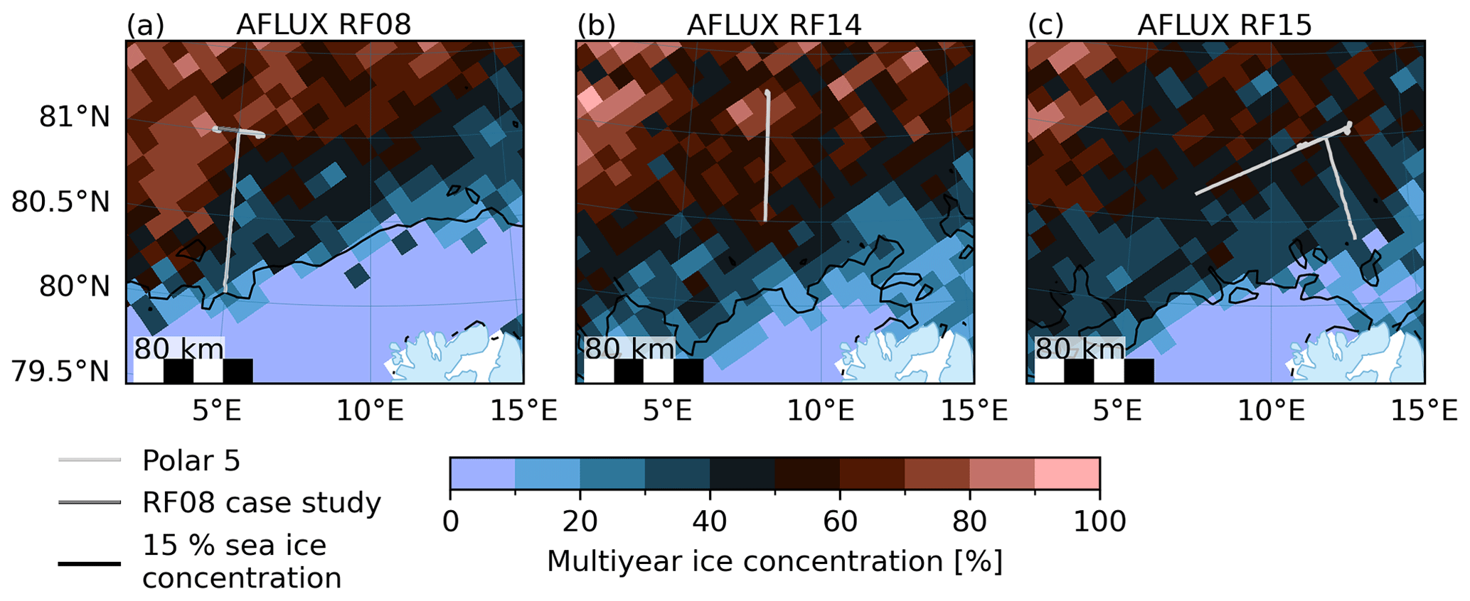
Figure A1 Maps illustrating the Polar 5 flight track; the sea ice edge, indicated by the 15 % sea ice concentration isoline (Spreen et al., 2008); and multiyear ice concentration (Melsheimer and Spreen, 2022) during (a) AFLUX RF08 (including the case study transect), (b) RF14, and (c) RF15.

Appendix B: Optimal number of k-means emissivity clusters

The k-means algorithm assigns a cluster to each normalized emissivity spectrum across the four MiRAC frequencies. Normalization involves subtracting the mean and scaling the emissivity of each channel to include unit variance, which ensures equal weighting between the four channels. However, the absolute number of clusters (k) is unknown and needs to be defined objectively. Therefore, we evaluate three metrics for cluster sizes ranging from 2–10 to identify the optimal k value (Fig. B1a). The distortion represents the sum of squared distances from all samples to their assigned cluster centroids (Thorndike, 1953). The distortion ideally follows an elbow-shaped curve, exhibiting a decrease until the optimal k value is reached and constant distortion for higher k values. The distortion curve for the emissivity samples flattens slightly after a k value of 4. The Calinski–Harabasz index determines the ratio of between-cluster dispersion to within-cluster dispersion, i.e., the ratio of separation to cohesion (Calinski and Harabasz, 1974). Higher Calinski–Harabasz index values correspond to optimal clustering with well-separated and dense clusters. The index peaks at a k value of 4 and decreases for both higher and lower values (Fig. B1a). The silhouette score represents the mean silhouette coefficient, which measures the similarity of a sample to its cluster compared to other clusters (Rousseeuw, 1987). Silhouette coefficients of 1 (−1) indicate correct (wrong) class assignment. On average, the silhouette score is 0.37 for 2–10 clusters. The silhouette score is highest for two clusters and shows a secondary peak at four clusters. All three metrics indicate that the emissivity spectra can be optimally divided into four clusters. The two-dimensional principal component analysis compression (Hotelling, 1933) shows the four identified emissivity clusters (Fig. B1b). Overall, the emissivity clusters are well separated, with gradual transitions occurring due to mixed types within the radiometer's footprint or transitional stages of the sea ice. Fish-eye lens images resolve these mixed types and transitional stages (Fig. B2).

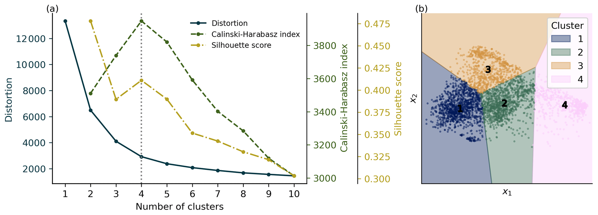
Figure B1 (a) The k-means clustering metrics – distortion, the Calinski–Harabasz index, and silhouette score – plotted as functions of the number of clusters. (b) Clustered emissivity spectra projected along the first two principal components (x₁, x₂) using k-means. The k-means cluster boundaries are approximated in a Voronoi diagram based on the cluster centroid projections. The cluster numbers are shown at the centroid positions.

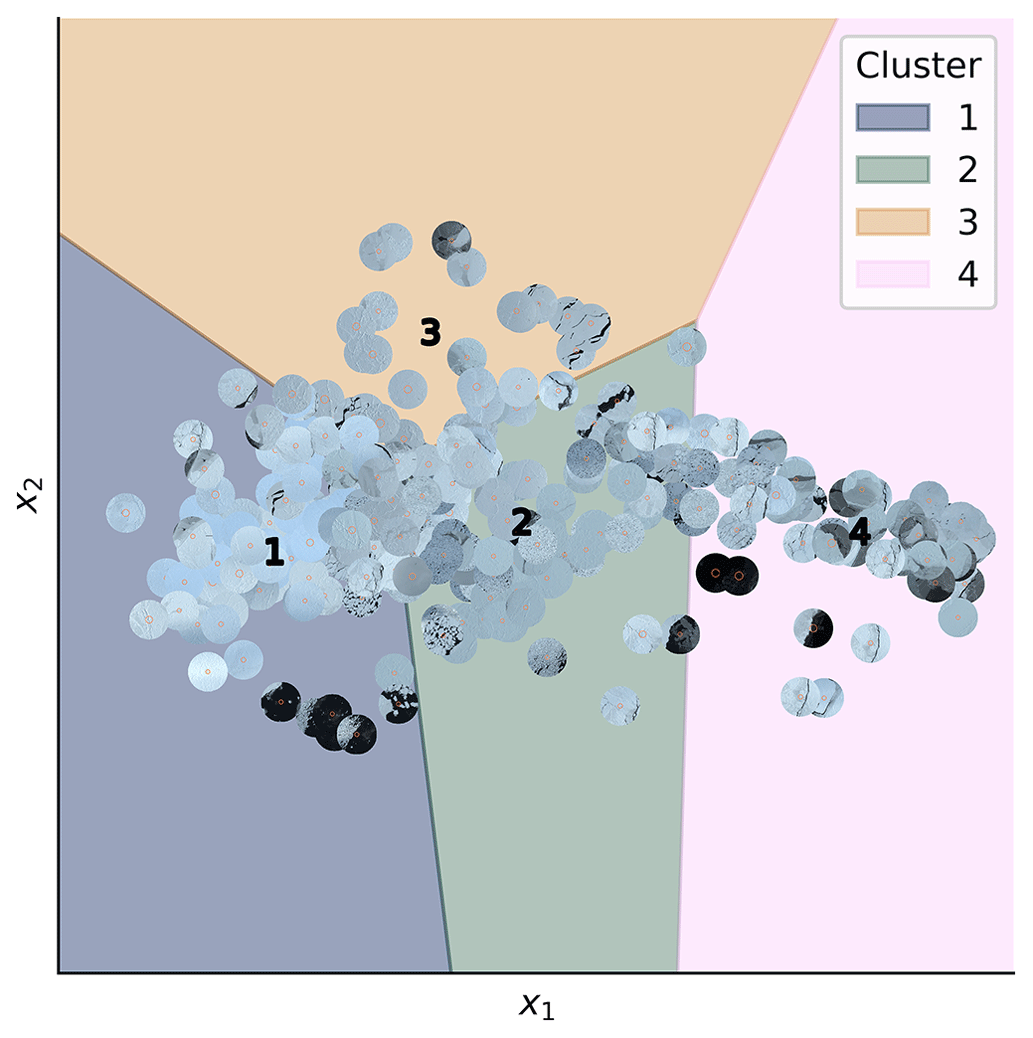
Figure B2 Fish-eye lens images corresponding to the emissivity samples shown in Fig. B1b. The k-means cluster boundaries are approximated in a Voronoi diagram based on the cluster centroid projections onto the first two principal components (x₁, x₂). The cluster numbers are shown at the centroid positions.

Appendix C: Sea ice emissivity spectra

We provide a figure of the MiRAC sea ice emissivity spectra and the k-means cluster centroids (Fig. C1).

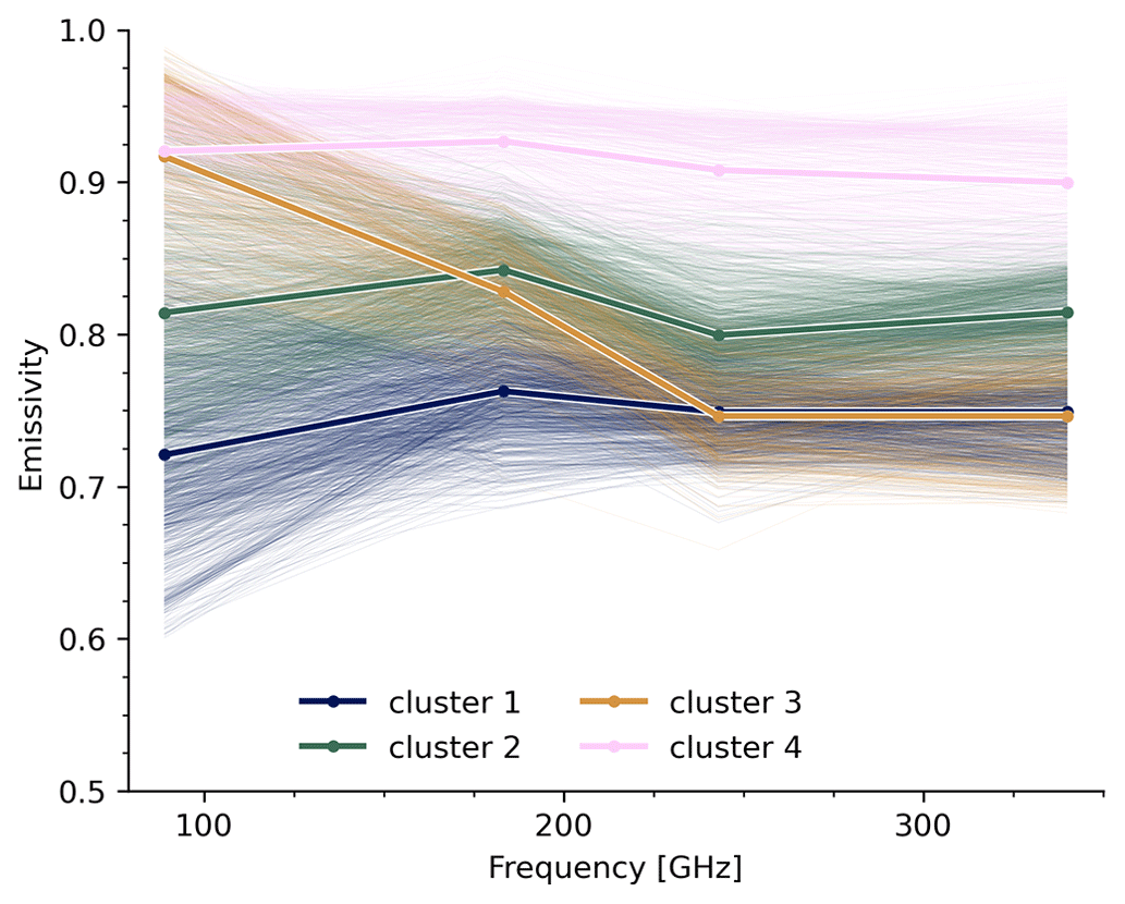
Figure C1 MiRAC sea ice emissivity spectra and k-means cluster centroids. Note that the 89 GHz channel measures horizontal polarization at an incidence angle of 25°, while the 183, 243, and 340 GHz channels measure it at nadir.