Evaluating different geothermal heat-flow maps as basal boundary conditions during spin-up of the Greenland ice sheet

There is currently poor scientific agreement on whether the ice–bed interface is frozen or thawed beneath approximately one third of the Greenland ice sheet. This disagreement in basal thermal state results, at least partly, from differences in the subglacial geothermal heat-flow basal boundary condition used in different ice-flow models. Here, we employ seven widely used Greenland geothermal heat-flow maps in 10 000-year spin-ups of the Community Ice Sheet Model (CISM). We perform two spin-ups: one nudged toward thickness observations and the other unconstrained. Across the seven heat-flow maps, and regardless of unconstrained or nudged spin-up, the spread in basal ice temperatures exceeds 10 ^∘C over large areas of the ice–bed interface. For a given heat-flow map, the thawed-bed ice-sheet area is consistently larger under unconstrained spin-ups than nudged spin-ups. Under the unconstrained spin-up, thawed-bed area ranges from 33.5 % to 60.0 % across the seven heat-flow maps. Perhaps counterintuitively, the highest iceberg calving fluxes are associated with the lowest heat flows (and vice versa) for both unconstrained and nudged spin-ups. These results highlight the direct, and non-trivial, influence of the heat-flow boundary condition on the simulated equilibrium thermal state of the ice sheet. We suggest that future ice-flow model intercomparisons should employ a range of basal heat-flow maps, and limit direct intercomparisons with simulations using a common heat-flow map.

1 Introduction

There is presently a tremendous diversity of opinion regarding the geothermal heat flow beneath the Greenland ice sheet due to a paucity of direct heat-flow measurements in the ice-sheet interior. While many subaerial, submarine, and shallow subglacial measurements have been made around the ice-sheet periphery, deep subglacial measurements have only been made at six deep ice coring sites in the interior (Camp Century, DYE-3, GRIP, GISP2, NGRIP, and NEEM). Consequently, the magnitude and spatial distribution of Greenland's subglacial geothermal heat flow remains poorly constrained across the seven unique Greenland heat-flow models presently in widespread use (Fig. 1) (Shapiro and Ritzwoller, 2004; Rezvanbehbahani et al., 2017; Martos et al., 2018; Greve, 2019; Lucazeau, 2019; Artemieva, 2019; Colgan et al., 2022). These individual geothermal heat-flow models are derived from multiple techniques that interpret a variety of geophysical variables (Table 1). We briefly discuss differences in the methodology and geophysical input variables of these existing heat-flow maps.

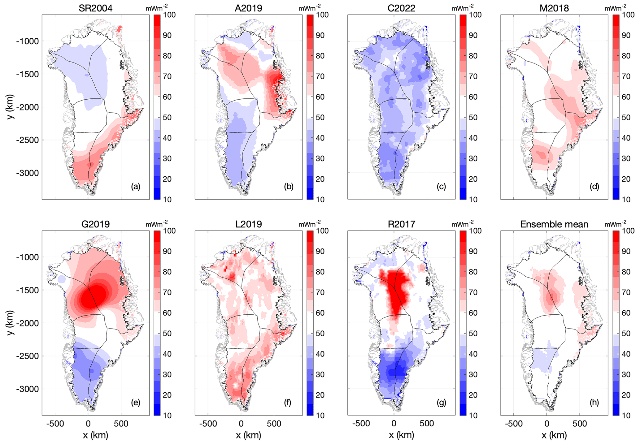
Figure 1 (a–g) The seven geothermal heat-flow maps considered as basal thermal boundary conditions. Color bars saturate about 10 and 100 mW m⁻². (h) Ensemble mean. Units for all plots, mW m⁻².

Table 1 Characteristics of the seven geothermal heat-flow models we explore as basal thermal boundary conditions: methodology used to derive each model, number of geophysical datasets employed by each model, number of in situ heat-flow observations considered by each model, average heat flow (± standard deviation) within a common CISM Greenland ice-sheet area, and the domain coverage of each model. Adapted from Colgan et al. (2022) and arranged from lowest to highest average geothermal heat flow beneath the ice sheet.

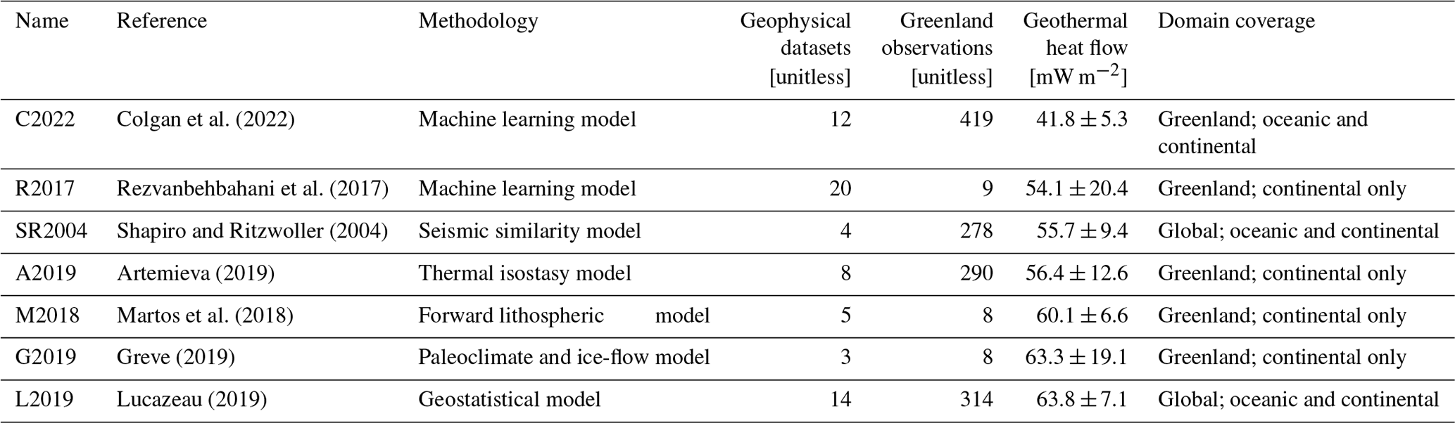
The Rezvanbehbahani et al. (2017) (R2017), Lucazeau (2019) (L2019), and Colgan et al. (2022) (C2022) heat-flow maps are perhaps methodologically most similar. These three maps use machine learning or geostatistics to predict heat flow as a function of diverse geophysical variables such as topography, tectonic setting, observed gravity, and magnetic field. They differ not only in the applied method but also in the set of geophysical variables utilized and their domains. Whereas Rezvanbehbahani et al. (2017) and Lucazeau (2019) only used global data, Colgan et al. (2022) substituted global datasets with Greenland-specific local data. By contrast, the Shapiro and Ritzwoller (2004) (SR2004), Martos et al. (2018) (M2018), and Artemieva (2019) (A2019) heat-flow maps all employ lithospheric models of varying complexity and more specific geophysical variables to infer heat flow. Shapiro and Ritzwoller (2004) correlate the seismic shear wave velocities of the upper 300 km with heat-flow observations and use this connection to predict heat flow from tomography data in areas without heat flow observations. Martos et al. (2018) use magnetic data to infer the Curie temperature depth, and the steady-state one-dimensional heat conduction equation, with lateral constant values for thermal conductivity and radiogenic heat production. Artemieva (2019) assumes an isostatic equilibrium and translates the corresponding topographic residuals to temperature anomalies which are then converted to a lithosphere–asthenosphere boundary undulation, and then uses individual reference geotherms for the different tectonic settings to derive the geothermal heat flow from lithosphere–asthenosphere boundary topography. Both methods then infer heat flow from the respective isotherms by applying a thermal model. The Greve (2019) (G2019) heat-flow map is unique in using paleoclimatic forcing of an ice-flow model to infer heat flow with a minimum of geophysical variables.

In North Greenland, there is especially poor agreement among the present generation of geothermal heat-flow models. Some models infer a widespread North Greenland high heat-flow anomaly (e.g., Greve, 2019), and some do not (e.g., Lucazeau, 2019). Other models offer products with and without this high heat-flow anomaly (e.g., Rezvanbehbahani et al., 2017). There are numerous secondary disagreements as well, including whether a model (1) infers traces of the Iceland Hotspot Track transiting from West to East Greenland (Martos et al., 2018), (2) infers elevated heat flow in East Greenland in closer proximity to the Mid-Atlantic Ridge (Artemieva, 2019), or (3) infers a low heat-flow anomaly associated with the North Atlantic Craton in South Greenland (Colgan et al., 2022).

Geothermal heat flow is a critical basal thermal boundary condition in Greenland ice-sheet models. It can significantly influence basal ice temperature and rheology, which in turn influences basal meltwater production and friction (Karlsson et al., 2021). Given the non-linear relation between ice temperature and rheology, and that most ice deformation occurs in the deepest ice layers, relatively small changes in basal ice temperature can result in large changes in ice velocity (Hooke, 2019). In extreme cases, diminished geothermal heat flow along subglacial ridges may contribute to the formation of massive refrozen basal ice masses (Colgan et al., 2021), or sharply enhanced geothermal heat flow may contribute to the onset of major ice-flow features (Smith-Johnsen et al., 2020).

Despite the clear links between geothermal heat flow and ice dynamics, a standardized geothermal heat flow as the basal thermal boundary condition was not prescribed in the Ice Sheet Model Intercomparison Project for CMIP6 (ISMIP6) (Goelzer et al., 2020). Of the 21 Greenland model submissions in ISMIP6, 12 prescribed geothermal heat flow according to Shapiro and Ritzwoller (2004), five prescribed it according to Greve (2019), two prescribed it as a hybrid assimilation of four older geothermal heat-flow models (Pollack et al., 1993; Tarasov and Peltier, 2003; Fox Maule et al., 2009; Rogozhina et al., 2016), and one prescribed a spatially uniform geothermal heat flow.

For Greenland, the ISMIP6 ensemble suggests that ∼ 40 % of the ice-sheet bed is frozen, meaning basal ice temperatures below the pressure-melting-point temperature, and ∼ 33 % of the ice-sheet bed is thawed, meaning basal ice temperatures at the pressure-melting-point (MacGregor et al., 2022). The ISMIP6 ensemble disagrees on whether the basal thermal state is frozen or thawed beneath the remaining ∼ 28 % of the ice sheet. It is unclear what portion of this disagreement is associated with the use of differing geothermal heat-flow boundary conditions across ensemble members. The geothermal heat-flow boundary condition can significantly influence the basal ice temperature and thus change the ice-flow rheology. For example, basal ice that is 1 ^∘C below pressure-melting-point temperature T_pmp deforms approximately 10 times more than ice 10 ^∘C below T_pmp at the same driving stress (Hooke, 2019).

In preparation for ISMIP7, there is a clear motivation to explore the choice of geothermal heat-flow boundary condition on modeled basal ice temperatures. Here, we spin up an ice-flow model with seven different geothermal heat-flow boundary conditions. This allows us to isolate the influence of the geothermal heat-flow boundary condition on the simulated thermal state and ice flow. We also discuss the pros and cons of these seven Greenland geothermal heat-flow products in the specific context of utility for future Greenland ice-flow simulations.

2 Methods

We use the Community Ice Sheet Model (CISM) (Lipscomb et al., 2019) as configured to spin up the Greenland ice sheet for ISMIP6 simulations (Goelzer et al., 2020). We run CISM on a regular 4 km grid with 10 vertical layers, using a higher-order velocity solver with a depth-integrated viscosity approximation (DIVA) based on Goldberg (2011). Note that the higher-order solver includes both membrane and vertical shear stress. All floating ice is assumed to calve immediately; thus we do not simulate Greenland's small floating ice shelves and ice tongues. For partly grounded cells at the marine margin, basal shear stress is proportionally weighted to the grounded fraction of the cell using a sub-grid grounding-line parameterization (Leguy et al., 2021).

We perform two types of ice-sheet spin-ups that we denote Case 1 and Case 2. The Case 1 spin-up iteratively nudges the friction coefficients in the basal-sliding power law to minimize misfit against observed present-day ice thickness. The nudging method is similar to that of Pollard and DeConto (2012) and was applied to the Antarctic ice sheet by Lipscomb et al. (2021). In this spin-up, we use a classic Weertman-type non-linear basal friction law (Weertman, 1979):

$$\begin{array}{}\text{(1)}& {\mathit{\tau }}_{\mathrm{b}}=C{\left|u_{\mathrm{b}}\right|}^{\mathrm{1}/\mathrm{m}-\mathrm{1}}{u}_{\mathrm{b}},\end{array}$$

where τ_b is the basal traction, u_b is the basal velocity, and m is a dimensionless constant that we set to 3. C is the spatially varying friction coefficient, in units of Pa yr m⁻¹, that is nudged during spin-up at each basal velocity point. The nudged C is capped at a maximum value of 10⁵ (implying high resistance to basal sliding) and a minimum of 10 (implying little resistance to sliding).

The spun-up ice thickness, by design, is close to observations. In most of the ice sheet, the thickness and velocity fields are in approximate balance, and thus the spun-up ice velocity also agrees well with observations, even though velocity is not a nudging target. The exceptions are regions where ice velocity has recently changed and ice thickness has not had time to adjust. The main drawback of the Case 1 spin-up method is that there is no dependence of basal sliding on basal temperature or water pressure. Thus, the method is not very physically based, and arguably overfits the ice thickness observations.

By contrast, the Case 2 spin-up is unconstrained, meaning that basal friction coefficients are not nudged to match the observed present-day ice thickness. We use a pseudo-plastic sliding law (Aschwanden et al., 2016):

$$\begin{array}{}\text{(2)}& {\mathit{\tau }}_{\mathrm{b}}=-{\mathit{\tau }}_{\mathrm{c}}{\displaystyle \frac{u_{\mathrm{b}}}{|u_{\mathrm{b}}{|}^{\mathrm{1}-q}{u_{\mathrm{0}}}^q}}\end{array}$$

where τ_c is the transient yield stress in Pa, q=0.5 is a dimensionless pseudo-plastic exponent, and u₀=100 m yr⁻¹ is a threshold speed. The yield stress is computed as ${\mathit{\tau }}_{\mathrm{c}}=N\tan \varnothing$, where N is the effective pressure and ∅ is a friction angle. The friction angle varies linearly as a function of bed elevation b between 40^∘ at b=700 m and 5^∘ at $b=-\mathrm{700}$ m. The effective pressure is computed from a local till model (Bueler and Van Pelt, 2015) and is sensitive to the thermal state of the bed; N is equal to the full overburden pressure ρ_igH (where ρ_i is the ice density, g is gravitational acceleration, and H is ice thickness) when the bed is frozen, but decreases to a small fraction (0.02) of overburden on thawed beds as the basal water depth rises to a capped value of 2 m. Lipscomb et al. (2019) provide more details.

While the Case 1 spin-up ice geometry closely matches present-day observations, there can be appreciable ice thickness biases for the non-nudged Case 2 spin-up. For ISMIP6, most participating models used data assimilation or nudged spin-ups to obtain a more accurate initial state. It is foreseeable, however, that future ISMIP protocols will encourage unconstrained spin-ups as a complement to nudged spin-ups, especially for simulations over multiple centuries during which basal conditions are likely to evolve. Unconstrained spin-ups are more physically based than nudged spin-ups in that the basal shear stress is closely tied to the modeled bed state (e.g., basal temperature, geology, and/or hydrology). It is more challenging, however, to reproduce a specific (i.e., present-day) ice-sheet configuration in an unconstrained spin-up.

For both Case 1 and 2 spin-ups, the ice sheet was initialized with present-day ice thickness and bed topography (Morlighem et al., 2017). The surface mass balance (SMB) and surface air temperature (T_air) are prescribed from a 1980–1999 climatology provided by the Modèle Atmosphérique Régional, a regional climate model (Fettweis et al., 2017). The initial englacial temperature was initialized to an idealized vertical profile. Where the prescribed SMB is negative, the initial temperature profile in each column is linear, with T= min(T_air, 0) at the surface and $T=T_{\mathrm{pmp}}-\mathrm{5}$ at the bed. Where the SMB is positive, the temperature is initialized to an analytic profile based on a balance between vertical conduction and cold advection (Cuffey and Paterson, 2010, Sect. 9.5.1). The ice sheet was then spun up for 10 000 years with a time step of $\mathrm{1}/\mathrm{6}$ year. The englacial temperature evolves under vertical conduction, horizontal and vertical advection, and deformational heating. Where the bed is frozen (T_b<T_pmp), the basal temperature is computed by prescribing a balance of geothermal heat flow, vertical conductive flux, and frictional fluxes at the ice–bed interface. Where the bed is thawed, meaning the resulting temperature would exceed T_pmp, we set T_b=T_pmp and use the excess energy to melt ice. By the end of the spin-up, the ice sheet is close to equilibrium (the relative change rate of ice volume is below 0.001 %), with transient englacial ice temperatures no longer influenced by the initial temperature profile.

We repeat the Case 1 and Case 2 spin-ups seven times each with the same configuration and execution, only varying the prescribed geothermal heat flow serving as the basal boundary condition (Table 1, Fig. 1). Each of the seven heat-flow maps is re-gridded from its native grid to the CISM grid using bilinear interpolation. For heat-flow maps that are only available onshore, meaning they omit offshore, or submarine, areas of the CISM domain, we similarly infill fjord heat-flow values using bilinear interpolation. These seven maps provide a diverse representation of the magnitude and spatial distribution of Greenland heat flow, with the mean heat flow within the CISM ice-sheet domain ranging from ∼ 42 mW m⁻² in the C2022 map to ∼ 64 mW m⁻² in the L2019 map. For R2017 we use the middle range scenario of NGRIP = 135 mW m⁻². For A2019, we use the “model 1” scenario, which adopts a deeper continental Moho depth than the “model 2” scenario. For C2022 we use their recommended “without NGRIP” scenario.

Of the seven heat-flow maps, only two are global maps (Shapiro and Ritzwoller, 2004; Lucazeau, 2019), and the remaining five are Greenland-specific. Of these five Greenland-specific maps, all but C2022 are limited to the onshore domain. The seven maps are evaluated against differing numbers of in situ heat-flow observations within a Greenland domain defined as <500 km from Greenlandic shores. The R2017, M2018, and G2019 heat-flow maps employed ≤9 primarily subglacial in situ observations from deep boreholes in the ice-sheet interior. The remaining four maps used significantly more in situ heat-flow observations (≥278), including more subaerial, submarine, and shallow subglacial measurements, associated with progressively improving versions of the International Heat Flow Database (Jessop et al., 1976; Fuchs et al., 2021).

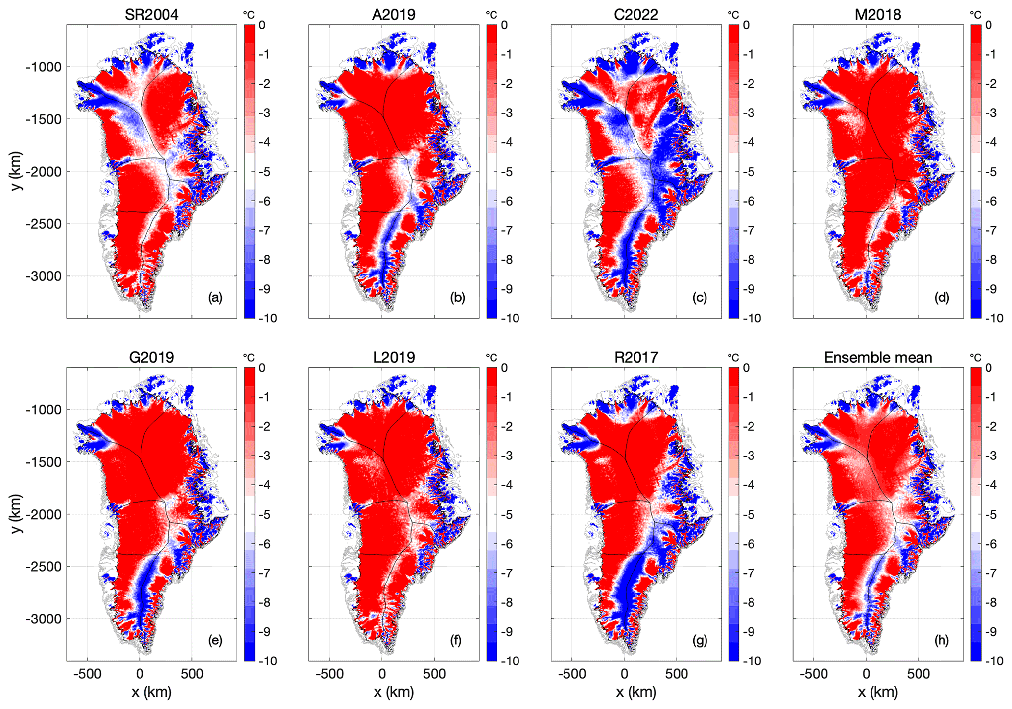
Figure 2 Case 1: (a–g) Ice-bed temperature relative to pressure melting point at transient equilibrium using the seven geothermal heat-flow maps. (i) Ensemble mean ice-bed temperature. Units in all plots ^∘C below pressure-melting-point temperature. (Compare against Case 2 in Fig. 9).

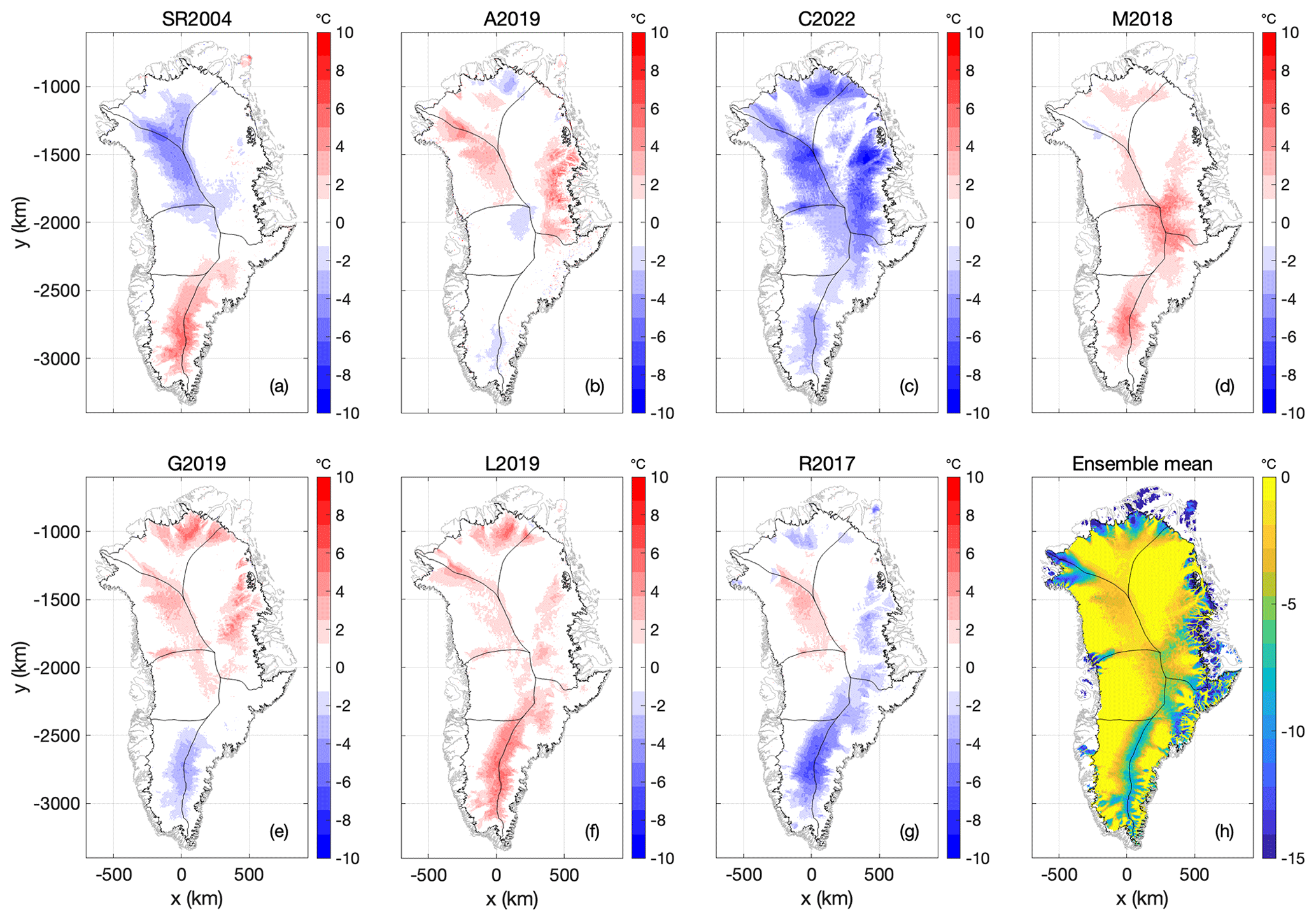
Figure 3 Case 1: (a–g) Relative anomaly from ensemble mean in ice-bed temperature relative to pressure melting point at transient equilibrium using the seven geothermal heat-flow maps. (h) Ensemble mean ice-bed temperature relative to pressure melting point. Units in all plots are ^∘C.

3 Results

3.1 Case 1 spin-up

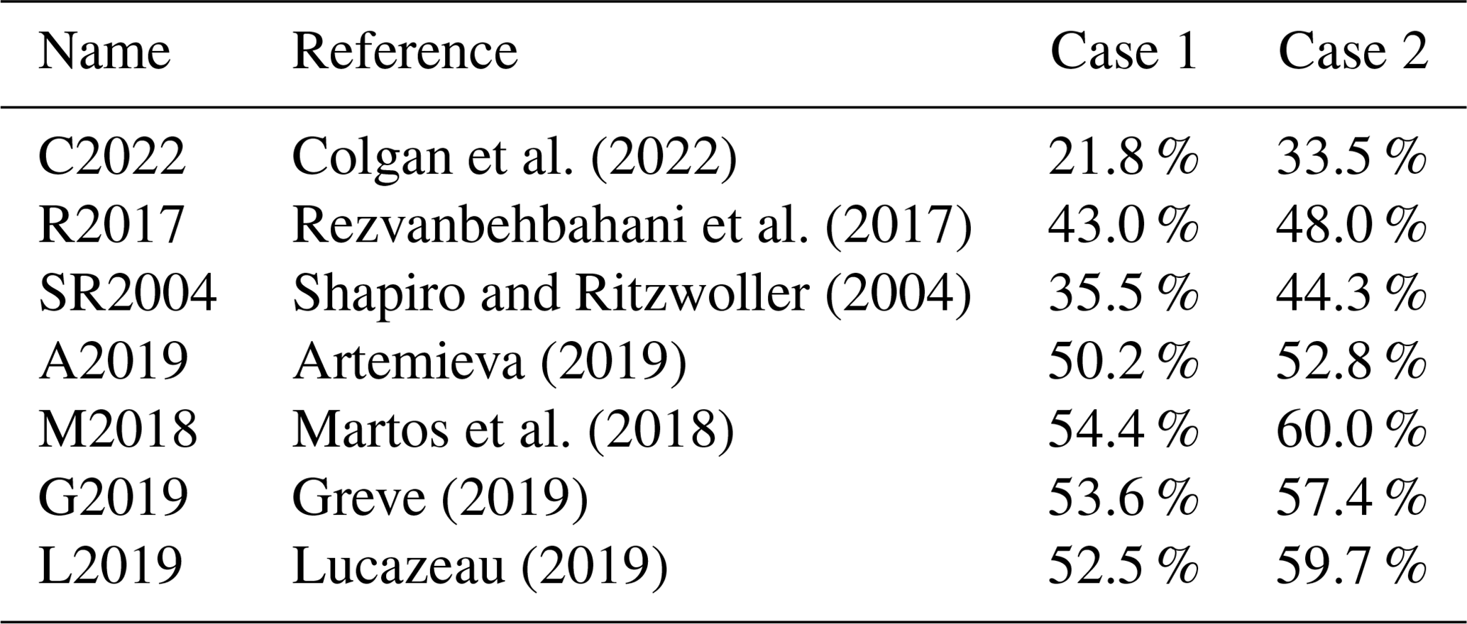
Figure 2 shows the ice-bed temperature T_b relative to T_pmp at the end of each Case 1 spin-up. The C2022 heat-flow map, which has the lowest mean geothermal heat-flow of all seven products, yields the smallest area of thawed basal temperatures (21.8 %) and the lowest basal temperature anomaly relative to the ensemble mean (Fig. 3; Table 2). Conversely, the relatively high M2018 heat-flow map, which has the third highest mean heat flow of all seven products, yields twice the area of thawed basal temperatures (54.4 %) and one of the highest basal temperature anomalies relative to the ensemble mean. Across the seven-member ensemble, however, there is considerable variation in the magnitude and spatial distribution of the ensemble spread in basal ice temperatures (Fig. 4). The seven heat-flow maps yield broadly similar modeled basal ice temperature RMSEs of between 1.0 and 2.8 ^∘C in comparison to observed basal ice temperatures at 27 Greenland ice-sheet boreholes (Fig. 5) (Løkkegaard et al., 2023).

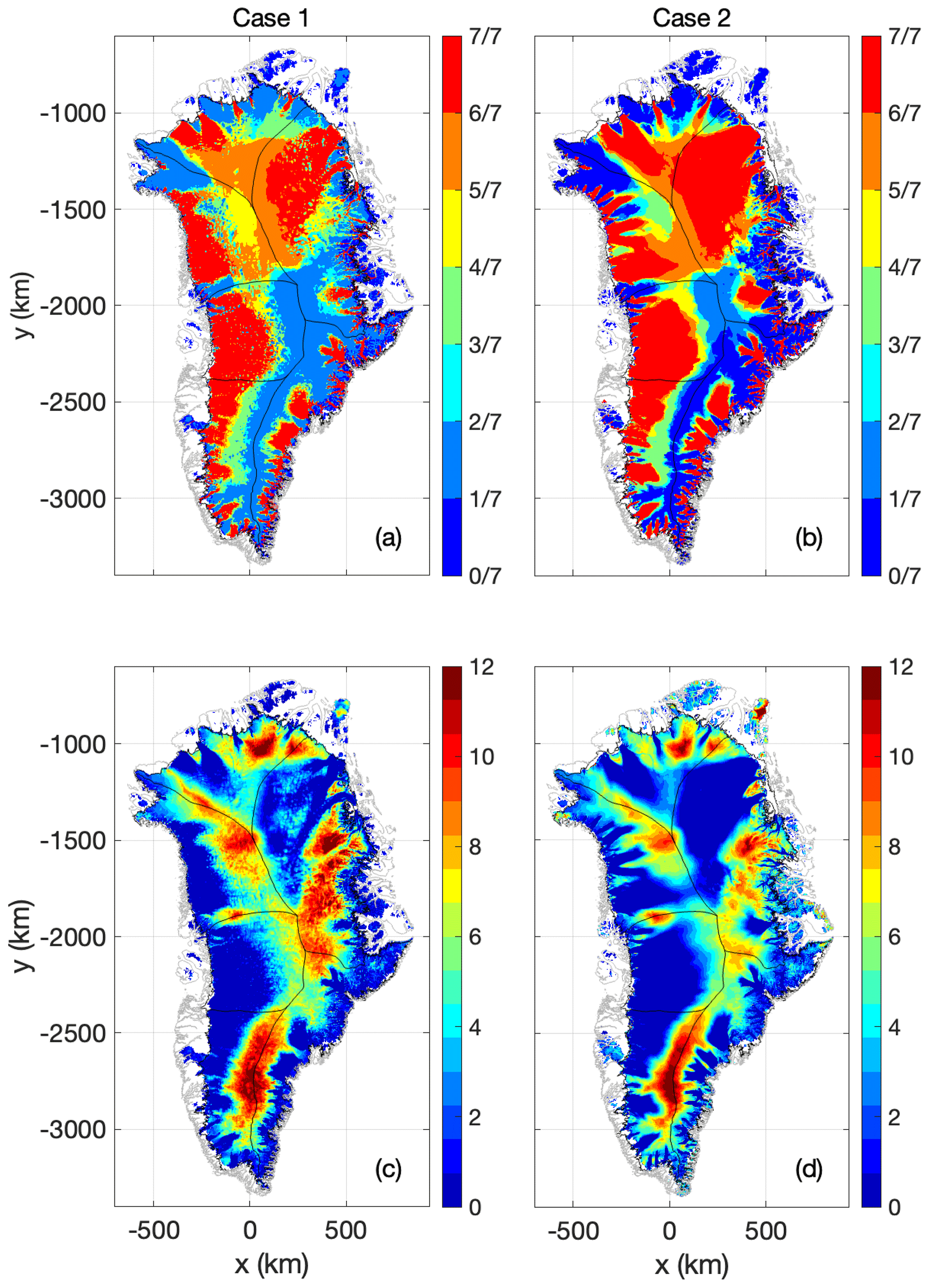
Figure 4 (a) and (b) Ensemble agreement in basal thermal state (frozen or thawed) across the seven heat-flow maps (a: Case 1, b: Case 2). Units are the fraction of simulations that suggest thawed bed. (c) and (d) Ensemble spread (the difference between maximum and minimum values for different experiments) in basal ice temperature across the seven heat-flow maps (c: Case 1, d: Case 2). Units are ^∘C.

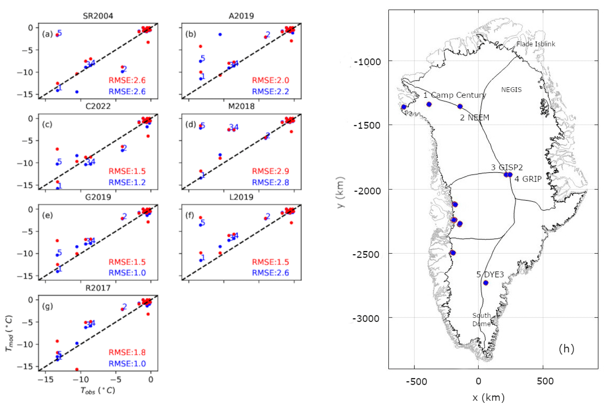
Figure 5 Modeled ice-bed temperature across the seven heat-flow maps versus observed ice-bed temperature at 27 Greenland ice-sheet boreholes where ice temperatures have been observed. (a–g) Modeled versus observed comparison across the seven geothermal heat-flow maps. The numbers show the deep ice core locations in (h). Case 1 spin-ups shown in blue. Case 2 spin-ups shown in red.

Table 2 Thawed-bedded ice-sheet area associated with Case 1 (nudged) and Case 2 (unconstrained) spin-ups of 10 000-year duration for the seven geothermal heat-flow datasets.

Generally, the ensemble spread in modeled ice-bed temperature approaches zero in the ablation area, especially in Central West Greenland, where the basal thermal state is thawed regardless of the heat-flow map. The ensemble spread is generally largest along the main flow divide of the ice sheet. At South Dome, the ensemble spread exceeds 10 ^∘C over an area of ∼ 10⁵ km². This highlights that the heat-flow map has a substantial influence on the simulated basal thermal state over the North Atlantic Craton. While the Northeast Greenland Ice Stream is thawed regardless of the heat-flow map, there is also an area of ∼ 10⁵ km² in Central East Greenland where the ensemble spread exceeds 10 ^∘C. Finally, the choice of heat-flow map appears to influence whether the North Greenland ablation area is thawed or frozen.

The Case 1 spin-up nudges the ice-flow model toward present-day ice thickness by iteratively adjusting basal friction coefficients C at each basal velocity point. The ensemble differences in C generally reach a maximum where ice velocities reach a minimum (Fig. 6). Perhaps counterintuitively, the highest surface ice velocities are associated with the lowest geothermal heat-flows (Fig. 7). For example, the high and low heat-flow end members of the L2019 and C2022 maps yield, respectively, low and high ice-velocity end members. Similarly, within the R2017 simulation, the low heat-flow anomaly in southeast Greenland yields a high ice-velocity anomaly. Accordingly, iceberg calving is highest in the lowest heat-flow simulations (Fig. 8). The relatively narrow ensemble spread in iceberg calving (∼ 1 %; 2 Gt yr⁻¹ ensemble range against 322 Gt yr⁻¹ ensemble mean) is ultimately constrained by the surface mass balance forcing at transient equilibrium when the ice sheet is adjusting during the spin-ups.

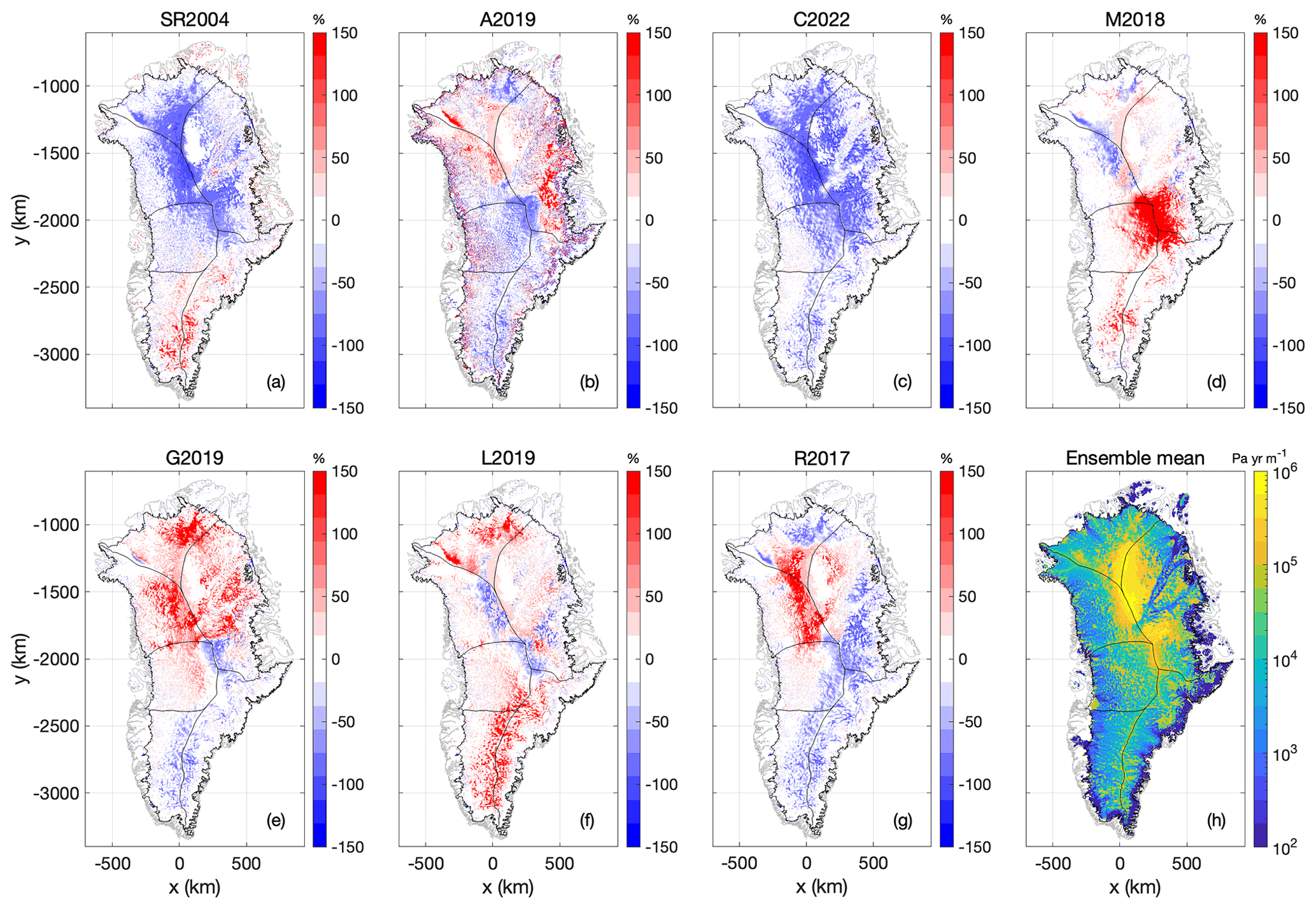
Figure 6 Case 1: (a–g) The basal friction coefficient at transient equilibrium using the seven geothermal heat-flow maps, expressed as anomalies from the ensemble mean. Units are % and color bars saturate at ±150 %. (h) Ensemble mean basal friction coefficient at transient equilibrium. Units are Pa yr m⁻¹, with the color bar saturating at 10⁶ Pa yr m⁻¹.

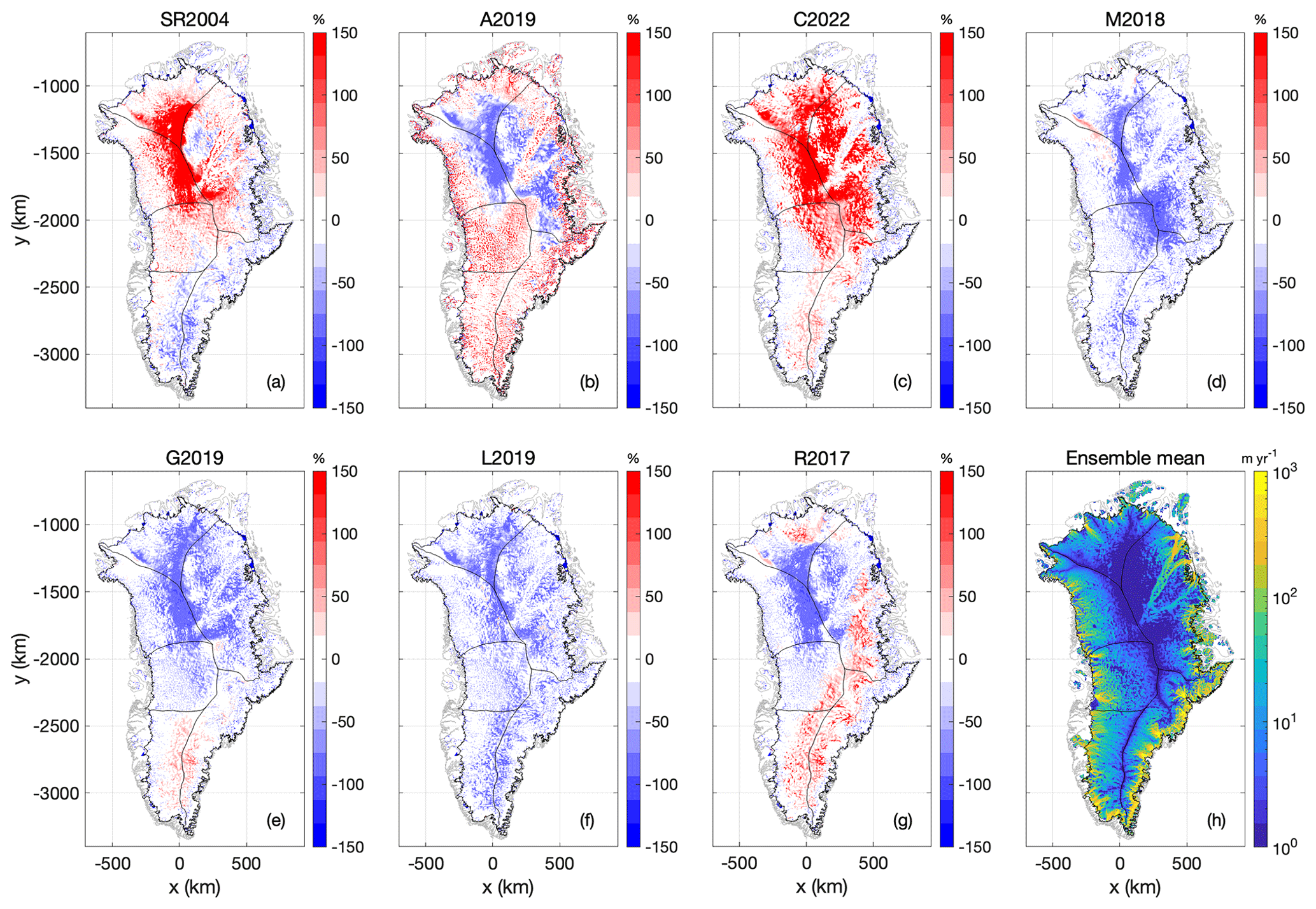
Figure 7 Case 1: (a–g) Surface ice velocity at transient equilibrium using the seven geothermal heat-flow maps, expressed as anomalies from their ensemble mean. Units are % and color bars saturate at ±150 %. (h) Ensemble mean surface ice velocity at transient equilibrium. Units are m yr⁻¹.

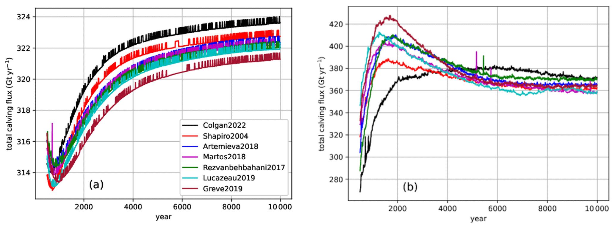
Figure 8 Total Greenland ice-sheet calving flux over the 10 000-year spin-up using the seven geothermal heat-flow maps for Case 1 (a) and Case 2 (b). Units are Gt yr⁻¹. The first 500 years of the simulations are not shown due to artifacts associated with model initialization.

3.2 Case 2 spin-up

Similar to the Case 1 spin-up, the Case 2 spin-up yields the smallest area of thawed basal temperatures (33.5 %) with the C2022 lowest mean geothermal heat-flow map and the largest area of thawed basal temperatures (60.0 %) with the M2018 relatively high mean geothermal heat-flow map (Fig. 9). Critically, the thawed-bed area for a given heat-flow map is consistently larger under the Case 2 (unconstrained) spin-up than the Case 1 (nudged) spin-up (Table 2). Basal ice temperatures are accordingly warmer under Case 2 than Case 1 (Fig. 10). As ice-sheet sensitivity generally increases with the thawed-bed area over which basal movement and subglacial hydrology can occur, this may suggest that unconstrained ice-sheet spin-ups are more sensitive than nudged ones. The apparent ice-temperature warming effect of an unconstrained spin-up appears to increase with decreasing heat flow. The shift toward warmer basal temperatures under Case 2 is most apparent for the C2022 heat-flow map, where the temperature difference is >5 ^∘C beneath a large portion of Central Greenland. All heat-flow maps yield large differences in basal ice temperature between Case 1 and Case 2 spin-ups in regions of fast ice flow around the ice-sheet periphery.

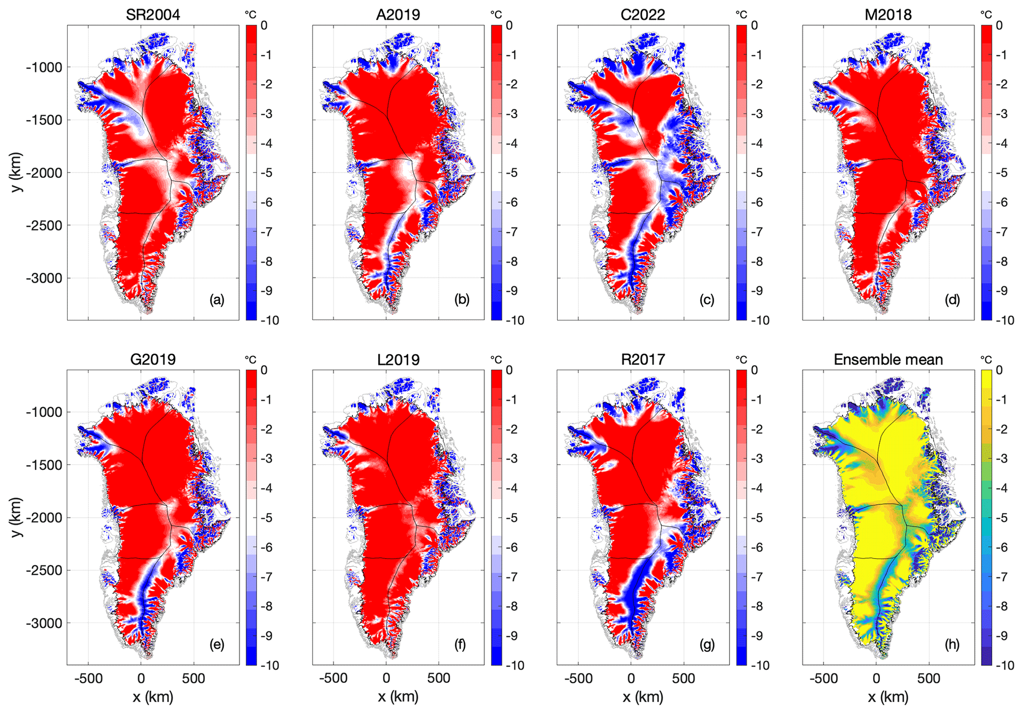
Figure 9 Case 2: (a–g) Ice-bed temperature relative to pressure melting point at transient equilibrium using the seven geothermal heat-flow maps. (h) Ensemble mean ice-bed temperature. Units in all plots ^∘C below pressure-melting-point temperature.

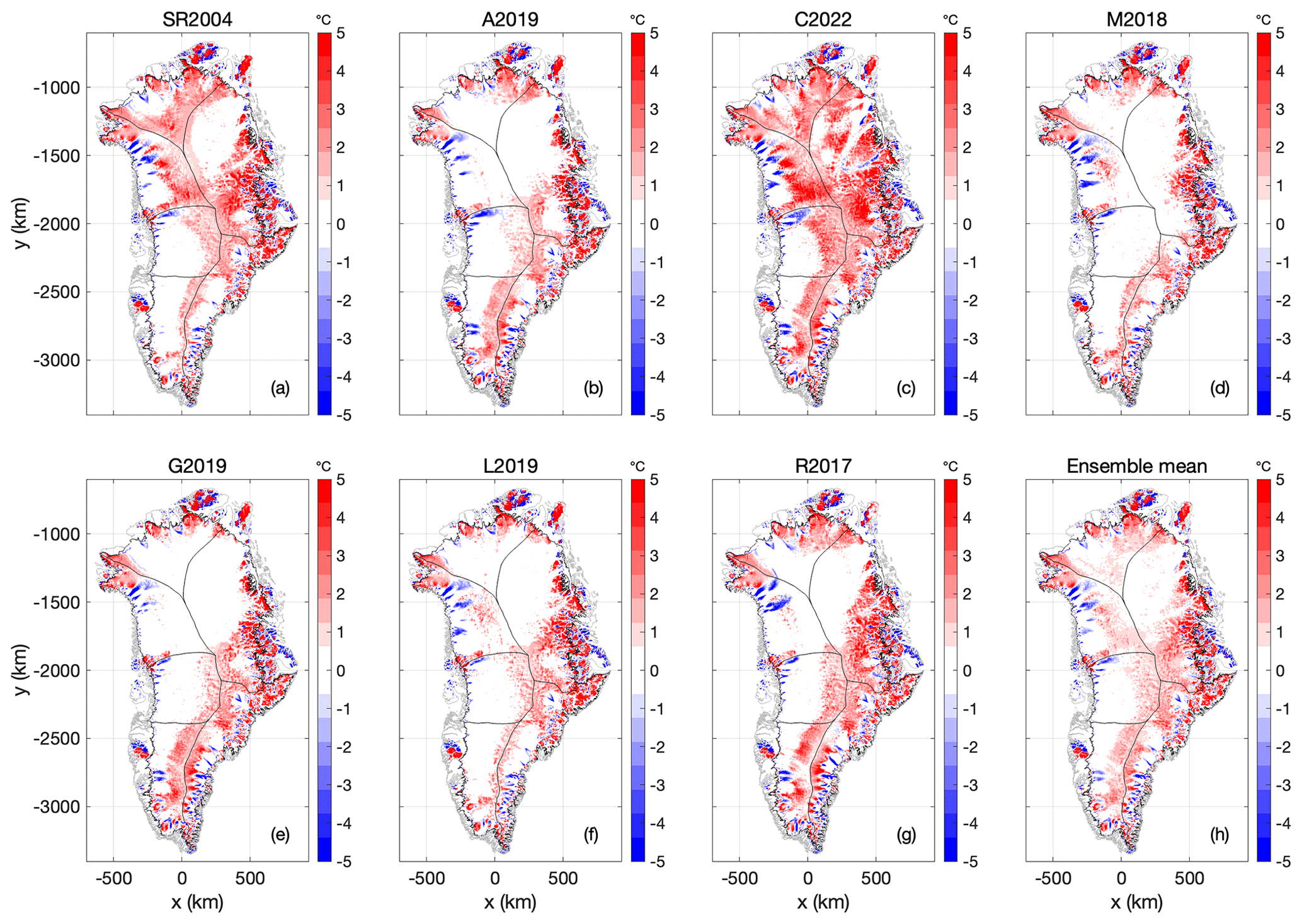
Figure 10 Case 2: (a–g) The difference of ice-bed temperature at transient equilibrium between Case 1 and 2 (T_Case2−T_Case1) using the seven geothermal heat-flow maps. (h) Ensemble mean for (a)–(g). Units in all plots are ^∘C.

The spatial pattern of the Case 2 ensemble agreement broadly follows that of Case 1 (Fig. 4), although the Case 2 agreement is generally poorer. This is attributable to the unconstrained nature of the Case 2 spin-up. The magnitude and spatial distribution of the ensemble spread in basal ice temperatures under Case 2 is largely similar to that of Case 1. The Case 2 ensemble spread is smaller in Central East Greenland and larger for peripheral ice caps, especially Flade Isblink in Northeast Greenland (Fig. 4). The Case 2 spin-up reproduces the observed basal ice temperatures at 27 Greenland ice-sheet boreholes with an RMSE of between 1.5 and 2.8 ^∘C (Fig. 5) (Løkkegaard et al., 2023). This is not significantly different from the RMSE range of the Case 1 spin-up. Basal ice temperatures are better resolved by the Case 1 spin-up for three heat-flow maps (C2022, G2019 and R2017), and better resolved by Case 2 for two maps (A2019 and L2019) with the remaining two maps yielding the same RMSE under both spin-ups (SR2004 and M2018). Empirical temperature observations therefore justify neither the Case 1 nor Case 2 spin-up approach.

In comparison with Case 1, the Case 2 spin-ups generally result in thicker ice in East Greenland and thinner ice in West Greenland (Fig. 11). These substantial differences in ice thickness (i.e., ±100 m) are clearly attributable to the unconstrained nature of Case 2 spin-up. Case 2 spin-ups with different heat-flow maps can yield very different ice thicknesses. For example, the SR2004 and C2022 maps yield substantially thicker than observed ice in North Greenland, where the G2019 and L2019 maps yield substantially thinner than observed ice. Similarly, the ice thickness at South Dome (South Greenland) varies considerably across the seven simulations. The magnitude of ice thickness differences associated with heat-flow maps is non-trivial, and the spatial distribution is complex.

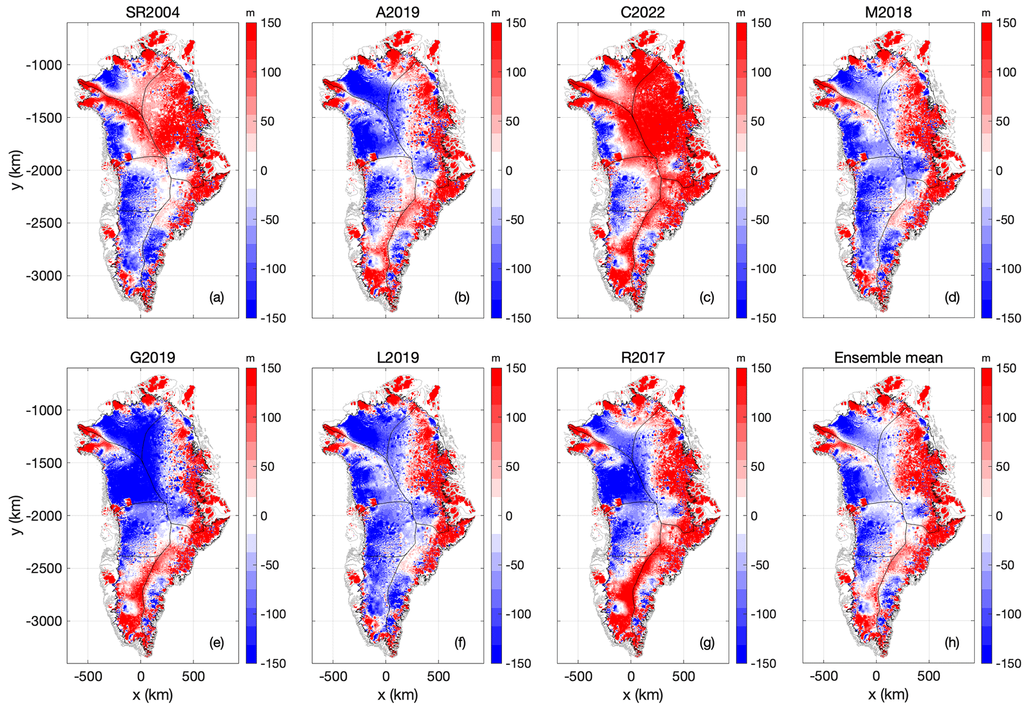
Figure 11 Case 2: (a–g) Anomaly in ice thickness at Case 2 transient spin-up, in comparison with Case 1 nudged spin-up, using the seven geothermal heat flow maps. Units in all plots are m and expressed as Case 2 minus Case 1. (h) Ensemble mean of ice thickness anomaly. The color bars saturate at ±150 m.

There are considerable velocity differences across the seven Case 2 spin-up simulations. Generally, these velocity differences appear to be negatively correlated with ice thickness differences (Fig. 12). For example, the SR2004 and C2022 heat-flow maps that yield substantially thicker ice in North Greenland also yield lower ice temperatures there. Similarly, the G2019 and L2019 maps that yield substantially thinner ice in North Greenland also yield faster velocities there. While relative velocity differences in the ice-sheet interior can appear striking in both magnitude and extent, there are also velocity differences around the ice-sheet periphery (Fig. 13), which strongly influences the iceberg calving from tidewater glaciers. Iceberg calving under Case 2 has a greater ensemble spread (∼ 5 %; 18 Gt yr⁻¹ ensemble range against 365 Gt yr⁻¹ ensemble mean) than under Case 1 (Fig. 8). Similar to Case 1, however, the C2022 lowest heat-flow map again has the highest iceberg calving flux, while the relatively high M2018 and G2019 heat-flow maps have substantially lower iceberg calving fluxes at equilibrium.

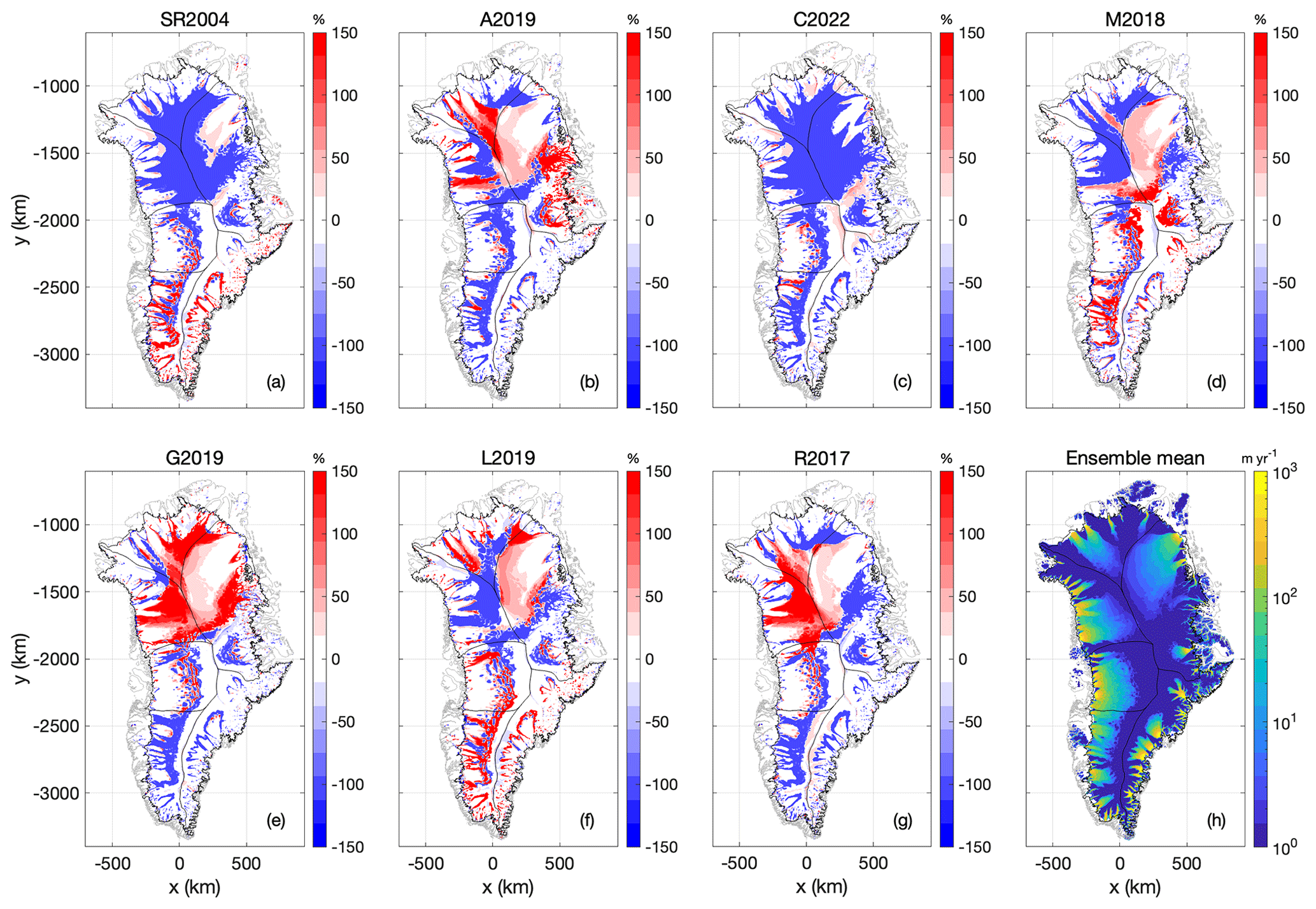
Figure 12 Case 2: (a–g) Surface ice velocity at transient equilibrium using the seven geothermal heat-flow maps, expressed as anomalies from their ensemble mean. Units are % and color bars saturate at ±150 %. (h) Ensemble mean surface ice velocity at transient equilibrium. Units are m yr⁻¹.

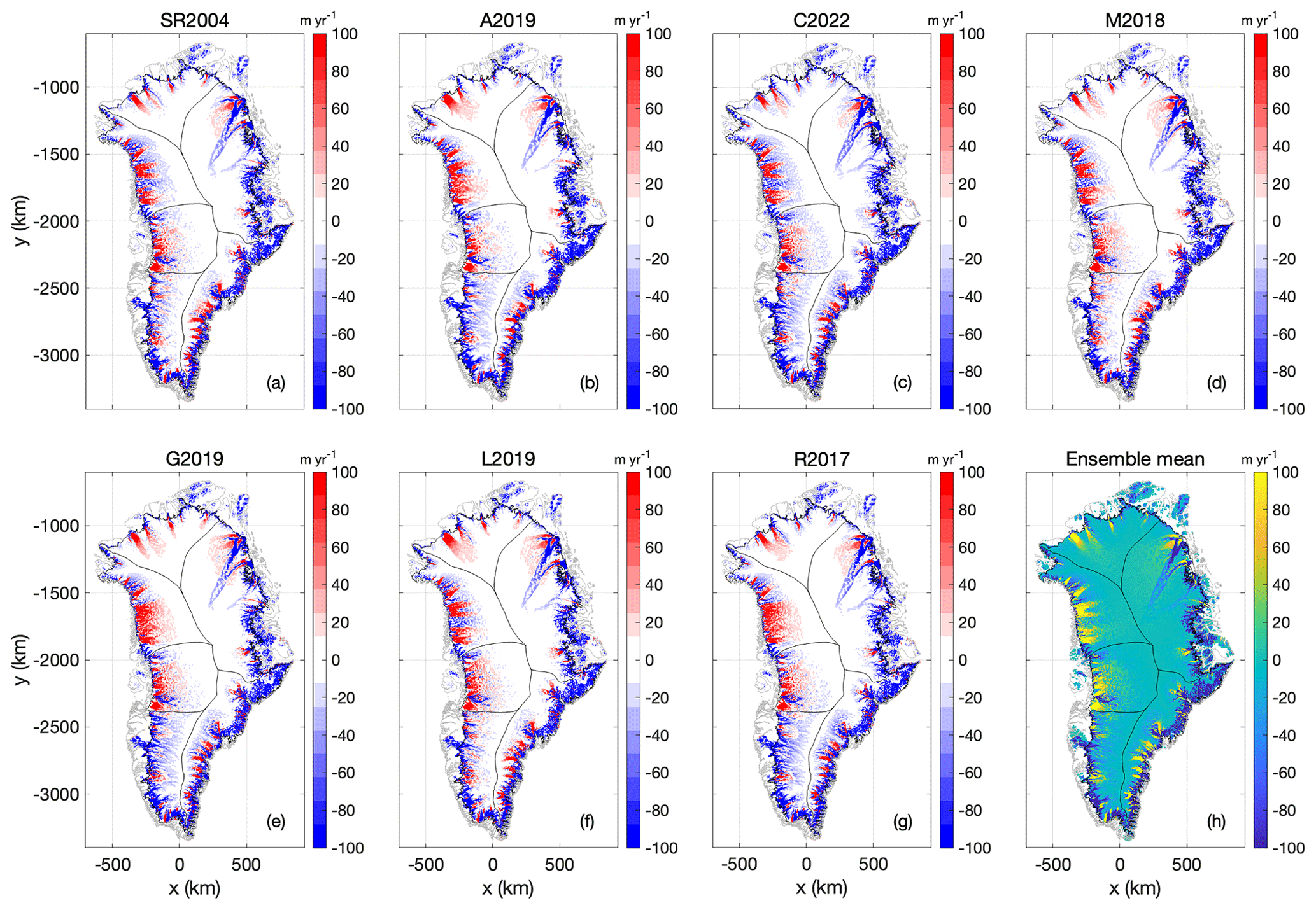
Figure 13 Case 2: (a–g) Anomaly in ice surface speed at Case 2 transient spin-up, in comparison with Case 1 nudged spin-up, using the seven geothermal heat-flow maps. Units in all plots are m and expressed as Case 2 minus Case 1. (h) Ensemble mean of ice surface speed anomaly. The color bars saturate at ±100 m yr⁻¹.

4 Discussion

The apparent association of higher ice velocities with lower geothermal heat flows under Case 1 appears to be a clear artifact of nudging the basal friction coefficient during spin-up. This effect has previously been described as the surface velocity paradox, whereby constraining an ice-flow model to match observed ice thickness results in underestimating deformational velocities where basal sliding is present, and overestimating deformational velocities where basal sliding is absent (Ryser et al., 2014). Avoiding this surface velocity paradox is the main motivation for the Case 2 spin-up, in which basal friction coefficients are not nudged. Under Case 2, there is more variation in the geometry, velocity, and thermal state of the ice sheet at the end of the 10 000-year spin-up. Perhaps counterintuitively, however, the highest iceberg calving fluxes remain associated with the lowest heat-flow maps (and vice versa for lowest iceberg calving fluxes). In unconstrained Case 2 simulations, this behavior cannot be attributed to a model artifact from the surface velocity paradox associated with nudging in Case 1. We instead speculate that a substantial portion of this variability simply reflects increased ice thicknesses under decreased heat flow.

The potential influence of anomalously high geothermal heat flow on contemporary local ice-sheet form and flow has been previously highlighted, with suggestions including the following: the onset of the Northeast Greenland ice stream may be associated with elevated geothermal heat flow (Fahnestock et al., 2001); there may be a feedback between deeply incised glaciers and topographic enhancement of local geothermal heat flow (van der Veen et al., 2007); and that the transit of the Iceland hotspot may have deposited anomalous heat into the subglacial lithosphere that influences ice flow today (Alley et al., 2019). Our evaluation suggests that knowledge of where anomalously low geothermal heat flow may be influencing contemporary regional ice-sheet form and flow can help constrain the choice of heat-flow map. For example, the widespread presence of Last Glacial Period ice in the ablation area across North Greenland suggests that heat flow must be sufficiently low to prevent basal melt across the region (MacGregor et al., 2020). This broad condition is only characteristic of a minority of the heat flow maps we evaluate, specifically the SR2004, R2017 and C2022 maps.

South Dome appears to be the most sensitive portion of the ice sheet to the choice of the geothermal heat-flow basal boundary condition. There, the choice of heat-flow map results in an ensemble spread in ice-bed temperature of >10 ^∘C over an area the size of Iceland. There is currently a poor level of scientific understanding of whether South Dome persisted through the Eemian interglacial, with some ice-sheet reconstructions suggesting persistence of the ice sheet's southern lobe (Quiquet et al., 2013; Stone et al., 2013) and others suggesting local deglaciation (Otto-Bliesner et al., 2006; Helsen et al., 2013). Our evaluation specifically highlights substantial disagreement over geothermal heat flow within the North Atlantic Craton that underlies South Dome. Similar to the contemporary persistence of Last Glacial Period ice in North Greenland, we speculate that paleo-ice-sheet simulations that adopt the low heat flow beneath South Dome characteristic of the R2017 map are more likely to yield an Eemian-persistent South Dome than paleo-ice-sheet simulations that adopt the high heat flow characteristic of the L2019 map. Simply put, the heat-flow map influences not only contemporary simulations of ice-sheet form and flow, but also paleo-ice-sheet simulations.We should note that, despite basal heat flow being a key factor in controlling ice dynamics, some other important physical processes (e.g., subglacial hydrology) are not considered in this study. The influence of different basal heat-flow models may not fully capture the role of enhanced basal meltwater in a warming climate. By holding basal friction coefficients fixed in time, Case 1 ignores the effects of evolving basal hydrology. Case 2 allows the thawed-bed area to change, but using a local till model that ignores subglacial water transport. Thus, Case 2 might be overly sensitive to local temperature changes, whereas more realistic hydrology changes would be spread over larger scales.

Furthermore, some higher-order ice-sheet models use data assimilation approaches (e.g., Hoffman et al., 2018) instead of spin-up, which may result in different model behaviors when applying different basal heat-flow datasets during initialization. Also, since our study focuses on the overall impacts of basal heat flow on Greenland ice-sheet dynamics, a more detailed understanding of the relative importance of thermal model components, such as ice frictional heating, heat advection and diffusion, is still required to improve the thermodynamic knowledge of the deep layers of the Greenland ice sheet.

5 Summary remarks

Given the non-linear dependence of deformational velocity on ice temperature, properly resolving the thermal state of the Greenland ice sheet is critical for generating reliable ice-flow simulations. We have performed both nudged and unconstrained ice-sheet spin-ups of 10 000-year duration with seven geothermal heat-flow models. Under a nudged spin-up, we find that the thawed-bed ice-sheet area ranges from 21.8 % to 54.4 % across these heat flow models. Under an unconstrained spin-up, the thawed-bed ice-sheet area is consistently larger, ranging from 33.5 % to 60.0 %. This suggests that unconstrained spin-ups generally yield a warmer Greenland ice-bed interface than constrained, or nudged, spin-ups. The unconstrained spin-up also yields inter-simulation differences in both ice thickness and velocity that are large in magnitude and extent. This ensemble of simulations highlights that sector-scale ice flow, both peripheral and interior, is at least moderately sensitive to the choice of heat-flow map.

The recent effort to compile all Greenland englacial temperature observations into a standardized database now permits the thermal state of ice-sheet simulations to be evaluated against all empirical data. Here, we evaluate simulated basal temperature against observed basal temperature at 27 selected Greenland boreholes. Despite the fact that the spatial resolutions of several basal heat-flow models are quite coarse in comparison with that of CISM, this evaluation still provides some insights on which heat flow map or spin-up approach is most locally suitable. Rather than quantitative comparisons against point temperature observations, however, there seems to be value in qualitative comparisons between heat-flow map and large-scale ice-sheet features, such as evaluating which heat-flow map can yield a widespread frozen bed in North Greenland under contemporary conditions. Naturally, evaluation of these seven heat-flow maps would be strengthened by using more than a single ice-flow model, as we do here.

Within our simulation ensemble, the unconstrained spin-ups may possibly be regarded as simulating more sensitive ice sheets than the nudged spin-ups, as the unconstrained spin-ups yield greater thawed-bed area and higher iceberg calving flux. While most recent ice-sheet simulations projecting Greenland's future sea-level contribution have focused on nudged spin-ups, our simulation ensemble unsurprisingly suggests that unconstrained spin-up is required to fully resolve the choice of geothermal heat-flow boundary condition on ice-sheet geometry and velocity. Given the strong influence of geothermal heat flow on ice dynamics that we document, it seems prudent to limit the direct intercomparison of ice-sheet simulations with those using a common heat-flow map. Similar to employing a range of commonly prescribed climate forcing scenarios, it would be ideal for future ISMIP ensembles to employ a range of commonly prescribed basal forcing conditions.