The role of atmospheric conditions in the Antarctic sea ice extent summer minima

Understanding the variability of Antarctic sea ice is still a challenge. After decades of modest growth, an unprecedented minimum in the sea ice extent (SIE) was registered in summer 2017, and, following years of anomalously low SIE, a new record was established in early 2022. These two memorable minima have received great attention as single cases, but a comprehensive analysis of summer SIE minima is currently lacking. Indeed, other similar events are present in the observational record, although they are minor compared to the most recent ones, and a full analysis of all summer SIE minima is essential to separate potential common drivers from event-specific dynamics in order to ultimately improve our understanding of the Antarctic sea ice and climate variability.

In this work, we examine sea ice and atmospheric conditions during and before all summer SIE minima over the satellite period up to 2022. We use observations and reanalysis data and compare our main findings with results from an ocean–sea ice model (NEMO–LIM) driven by prescribed atmospheric fields from ERA5. Examining SIE and sea ice concentration (SIC) anomalies, we find that the main contributors to the summer minima are the Ross and Weddell sectors. However, the two regions play different roles, and the variability of the Ross Sea explains most of the minima, with typical negative SIE anomalies about twice as large as the ones in the Weddell Sea. Furthermore, the distribution of SIC anomalies is also different: in the Weddell Sea, they exhibit a dipolar structure, with increased SIC next to the continent and decreased SIC at the sea ice margin, while the Ross Sea displays a more homogenous decrease. We also examine the role of wintertime sea ice conditions before the summer SIE minima and find mixed results depending on the period: the winter conditions are relevant in the most recent events, after 2017, but they are marginal for previous years. Next, we consider the influence of the atmosphere on the SIE minima, which is shown to play a major role: after analyzing the anomalous atmospheric circulation during the preceding spring, we find that different large-scale anomalies can lead to similar regional prevailing winds that drive the summer minima. Specifically, the SIE minima are generally associated with dominant northwesterly anomalous winds in the Weddell Sea, while a southwesterly anomalous flow prevails in the Ross Sea. Finally, we investigate the relative contribution of dynamic (e.g., ice transport) and thermodynamic (e.g., local melting) processes to the summer minima. Our results indicate that the exceptional sea ice loss in both the Ross and Weddell sectors is dominated at the large scale by thermodynamic processes, while dynamics are also present but with a minor role.

1 Introduction

Unlike its counterpart in the Northern Hemisphere, Antarctic sea ice extent has started to display signs of a decrease only during the last few years, after a period of overall increase between 1979 and 2016 (e.g., Parkinson and Cavalieri, 2012; Hobbs et al., 2016; Parkinson, 2019). While it is still unclear whether this is the start of a new trend or just part of the short-term variability, it is certain that the recent period has witnessed some unprecedented events, such as the new record low of sea ice extent (SIE) in early 2022. After a retreat that was quicker than usual (Raphael and Handcock, 2022), a record value of 1.92×10⁶ km² was registered on 25 February (Thompson, 2022), almost 1×10⁶ km² below the climatology. This value established a new absolute minimum in the historical record since its predecessor, in 2017, was higher than the symbolic threshold of 2×10⁶ km² (e.g., Raphael and Handcock, 2022). Even after the growth season and for the rest of 2022, the SIE maintained exceptionally low values, and a subsequent, deeper summer minimum was observed in early 2023 (Liu et al., 2023; Purich and Doddridge, 2023), with strong negative anomalies still continuing at the time of this paper.

The February 2022 episode received immediate attention from the scientific community, which did not wait long to provide the first detailed description of the event (Thompson, 2022) and preliminary hypotheses on its causes (Raphael and Handcock, 2022). More detailed studies followed shortly after, which investigated the physical drivers and potential mechanisms leading to these extreme conditions. Wang et al. (2022) found that the summer SIE minima arose mostly from negative sea ice concentration (SIC) anomalies in the southwestern Amundsen Sea, southeastern Ross Sea and northwestern Weddell Sea. They highlighted the contribution of a deepened Amundsen Sea Low (ASL) already during the preceding spring, which was in turn favored by a positive phase of the Southern Annular Mode (SAM). As a result, increased poleward heat transport was found in the Weddell Sea due to anomalous northerly winds on the eastern flank of the ASL, which also pushed more sea ice towards the continent. Concurrently, southerly winds on the western flank of the ASL transported more sea ice towards lower latitudes, favoring melting in the Ross Sea. Furthermore, the authors attributed the negative SIC anomalies to a combination of dynamics and thermodynamics in spring and to mostly thermodynamic processes in summer. Similar results were obtained by Turner et al. (2022), who further stressed the influence of the anomalously deep ASL on the summer SIC anomalies in the Weddell and Ross seas; additionally, they emphasized the role of a series of intense storms passing in late spring and early summer. More recently, Yadav et al. (2022) specifically focused on the atmospheric precursors of this event during the preceding months, i.e., since September 2021. They highlighted that record SIE values were already registered during the period November–January. Similarly to the other two studies, they also suggested a key role of the ASL, in conjunction with the SAM, during both spring and summer. In addition, they observed a strengthening of the stratospheric polar vortex that could have favored the large-scale tropospheric anomalies.

The previous record minimum in summer 2017 was even more surprising, as it interrupted the modest but robust SIE growing trend of the previous decades (e.g., Zwally et al., 2002; Simmonds, 2015; Comiso et al., 2017), which culminated in an all-time maximum in 2014 (e.g., Massonnet et al., 2015). Furthermore, the summer minimum was preceded by a dramatic decrease already in late spring 2016, which was the focus of most studies (e.g., Turner et al., 2017). This event appeared to be driven by both the ocean and atmosphere (Stuecker et al., 2017; Schlosser et al., 2018; Meehl et al., 2019; Zhang et al., 2022), including the stratosphere (Wang et al., 2019), as suggested by observations and climate model simulations (e.g., Kusahara et al., 2018; Purich and England, 2019). It resulted from an exceptionally early and rapid ice retreat during the melt season, accompanied by atmospheric circulation anomalies in different sectors, that culminated in November 2016 and continued until March 2017. Similar to 2022, SIE anomalies mainly emerged in the Ross and Weddell seas, though the spring anomalies were also present in other regions. However, the large-scale atmospheric circulation appeared to be quite different from the one observed in 2022. In early spring, the atmosphere over the Southern Ocean was dominated by a positive phase of the zonal wave 3 (ZW3) pattern, followed by an almost record negative SAM, while the ASL showed no persistent deepening. Additionally, surface and sub-surface ocean conditions played a minor role in driving the minimum itself but contributed to the persistent SIE decline that started in early 2016 (e.g., Zhang et al., 2022).

The 2022 and 2017 minima are widely discussed in the literature as single cases, but only a few studies have compared them to each other (e.g., Wang et al., 2022) or to other similar events (e.g., Turner et al., 2022). Furthermore, most of these works are based on observations, with limited variables available, and no modeling study for 2022 has been carried out to our knowledge. Unusual anomalous values were also registered during other years and seasons (e.g., Jena et al., 2022), but they received less attention as they did not lead to such an extreme absolute SIE. However, analyzing other SIE minima, although minor compared to the recent ones, is essential to further comprehending the dynamics of sea ice variability, to understanding the relation between extreme events and atmospheric and ocean conditions, and to potentially interpreting the latest records as isolated events or as being part of long-term trends.

In this work, we carry out a comprehensive study of SIE minima over the whole satellite observational period up to 2022, which is currently lacking. In particular, we focus on summer events, since they typically correspond to absolute yearly minima due to the seasonal cycle of sea ice. It is evident that the two most recent and striking events of 2017 and 2022 present some similarities, such as the regional patterns of SIC anomalies; however, they are very different in terms of atmospheric and possibly ocean precursors. Thus, here we compare them to other SIE minima and highlight common features versus event-specific processes. We focus on the atmosphere and examine the large-scale conditions over the Southern Ocean related to the summer SIE minima but without considering explicitly potential remote drivers and forcings, as in previous works. Instead, we analyze the role of anomalous winds in driving sea ice changes in different regions and the associated processes and also consider the impact of the previous winter sea ice conditions. In contrast, we do not explore here the contribution from the ocean: while it may have a clear influence on the persistence of the anomalous conditions, it has been shown that its role is minor compared to the atmospheric forcing for the peak of the 2017 and 2022 minima (e.g., Schlosser et al., 2018; Kusahara et al., 2018; Turner et al., 2022; Zhang et al., 2022). This study is based on observations and reanalysis data but also examines results from an ocean–sea ice model driven by observed atmospheric fields.

After presenting the data and methods in Sect. 2, we examine the summer SIE time series and discuss the SIC anomalous patterns during years defined as “minima” (Sect. 3.1 and 3.2) and consider the influence of the sea ice state in the previous winter (Sect. 3.3). Then, we investigate the atmospheric circulation anomalies during the preceding spring, both at a large scale and regionally, by focusing on the prevailing local wind direction (Sect. 3.4). Using a model allows us not only to derive more robust conclusions but also to further investigate the processes at play thanks to output variables that are not available for the observations. For instance, in Sect. 3.5 we estimate the contribution to anomalous sea ice changes from dynamic and thermodynamic processes by means of online diagnostics in the model. The main findings are summarized and discussed in Sect. 4.

2 Data and methods

2.1 Observations and model

We use observed daily SIC from the EUMETSAT Ocean and Sea Ice (OSI) Satellite Application Facility (SAF) datasets (OSI-450 and OSI-430-b; OSI SAF, 2017; Lavergne et al., 2019) and monthly 10 m wind and sea level pressure (SLP) from the ERA5 reanalysis (Hersbach et al., 2020) over the period 1980–2022.

We compare the observations with results from a regional ocean–sea ice model forced by atmospheric conditions from reanalyses over the same period. The ocean model is NEMO3.6 (Nucleus for European Modeling of the Ocean; Madec et al., 2017) coupled to the sea ice model LIM3.6 (Louvain-la-Neuve sea ice model; Vancoppenolle et al., 2012; Rousset et al., 2015) in a regional configuration that covers the Southern Ocean (SO) from 30° S. The horizontal resolution is close to $\mathrm{1}/\mathrm{4}$° (about 24 km at the 30° S boundary and 14 km at 60° S), and there are 75 vertical levels, with thickness increasing from 1 m at the surface to about 200 m at depth. In this simulation, ranging from January 1980 to March 2022, the model is driven by atmospheric fields from ERA5 over the SO domain and forced at the ocean boundaries with observations from the ORAS5 oceanic reanalysis (Zuo et al., 2019), while the initial conditions are set using the climatology (1990–2009) from a previous run.

A full description and evaluation of the model can be found in Pelletier et al. (2022; specifically, we use the same configuration as in their PAROCE experiment). Documented issues include systematic biases in the SIE seasonal cycle, which are related to well-known NEMO–LIM features (Vancoppenolle et al., 2012; Rousset et al., 2015). Particularly, the simulation used here reproduces the observed growth from March to July well (Fig. S1 in the Supplement) but eventually overestimates the extent around the winter peak (1.1×10⁶ km² more than the observations in September). Very little melting occurs before November, after which a steep decrease follows, with most of the melting happening between December and January. Due to the excessive winter extent and the short melting season, December is also the month with the strongest bias in the mean SIE, with a difference between the model and the observations of about 4.4×10⁶ km². In summer, in contrast, too little sea ice is left in the model. A lack of 1.9×10⁶ km², compared to the observations, is typically present in February, while the difference is smaller in January and March (the average January–March bias is −1.5 km²). The positive winter SIE bias is mostly related to a sea ice excess in the Bellingshausen Sea–Amundsen sector and eastern Indian Ocean–western Pacific Ocean, but the Ross Sea also contributes (Fig. S2). In summer, a lack of SIC is observed in almost all sectors. Particularly relevant for this study is the fact that the Ross Sea is virtually ice-free in February and that a substantial portion of sea ice is also missing in the western Weddell Sea through the whole season. In the eastern Weddell sector, in contrast, the model systematically overestimates the SIC and extent, particularly in January.

2.2 Methods

We select summer minima common to the model and observations based on January–March (JFM) anomalies of the SIE. We use the standard definition of SIE based on a 15 % threshold for SIC. To simplify the selection of the events, we consider the standardized time series by dividing the anomalies by their standard deviation (σ) over the whole period. We first identify circumpolar (hereafter “total”) minima using the full SIE computed for the whole SO domain and by selecting those years with anomalies below −1σ in the observations and below −0.5σ in the model. With this definition, all the events below −1σ in the observations are selected as minima (Fig. 1a), but we ensure that concurrent substantial negative SIE anomalies occur in the model and are worth exploring further for physical mechanisms (note that considering 1σ also for the model would lead to the selection of only two events). A similar approach is used with the SIE computed only in the Ross sector (160° E–130° W; see Fig. 2f) to identify years that are regional minima, which may not correspond to the ones of the total SIE, as discussed in Sect. 3.1. For the Weddell sector (60° W–20° E; see Fig. 2f), a slightly different definition is applied due to the smaller SIE variability in that region (see Fig. 1c). A year is selected as a minimum in the Weddell Sea if (i) the SIE time series of the observations falls below −1σ and the time series of the model is concurrently below −0.5σ or (ii) the SIE time series of the model falls below −1σ and the time series of the observations is concurrently below −0.5σ. We choose to focus on the JFM seasonal mean (see climatology in Fig. S3) because the absolute minima can occur in both February (as in 2022; see Thompson, 2022) and March (as in 2017; see Turner et al., 2017) and also because of the model's bias discussed above, which is stronger in February.

The anomalies are computed with respect to the climatology of the entire period (1980–2022). The statistical significance of the composites is assessed with bootstrapping by building 500 synthetic composites with the same number of years randomly sampled from the same period. The threshold for significance is set to 90 %.

2.3 Sea ice concentration budget

The SIC evolves over time in response to a variety of processes, which can be categorized as thermodynamic or dynamic. New ice formation in open waters and ice melt are thermodynamic processes increasing and decreasing the SIC, respectively. Vertical processes in the sea ice such as bottom growth, bottom melt, surface melt and snow ice formation are also thermodynamic contributors to SIC changes, directly or through their impact on the sea ice thickness. The dynamic processes that influence SIC are essentially related to the sea ice velocity (u), which is in turn driven by ocean drag and, mostly, wind stress. These processes include contributions from sea ice advection (u⋅∇SIC) and divergence (SIC ∇⋅u). The advection represents the local import (export) of sea ice, effectively increasing (decreasing) the local SIC, while the divergence encapsulates how the sea ice motion leads to openings (closures) in the pack, thus leading to a local decrease (increase) in SIC. Additionally, other mechanisms like mechanical redistributions (e.g., ridging, rafting) also act as dynamic drivers of SIC variations. In our model, at each time step and grid point, the simulated total change in SIC (tendency) is split into thermodynamic and dynamic contributions:

$$\begin{array}{}\text{(1)}& {\displaystyle \frac{\mathrm{dSIC}}{\mathrm{d}t}}={{\displaystyle \frac{\mathrm{dSIC}}{\mathrm{d}t}}}_{\mathrm{thermo}}+{{\displaystyle \frac{\mathrm{dSIC}}{\mathrm{d}t}}}_{\mathrm{dyn}}.\end{array}$$

The first term represents the change in SIC due to thermodynamics (thermo), while the second term includes the contribution of all dynamic (dyn) processes accounted for in the model (e.g., Barthélemy et al., 2018). In Sect. 3.5., we use these diagnostics to evaluate the contribution of dynamic and thermodynamic processes to the summer SIE minima.

A similar tool developed for observations by Holland and Kwok (2012) uses different definitions. The SIC tendency is computed explicitly as the difference between successive time steps. The dynamic term corresponds to the sum of SIC advection and divergence, which are computed directly using observed sea ice motion vectors. Then, the difference between these two terms is a residual that is attributed to thermodynamics and other secondary processes, including redistribution mechanisms. While this diagnostic was used in successive works to analyze climatologies and trends and even applied to numerical model outputs (e.g., Lecomte et al., 2016; Holmes et al., 2019), it relies on sea ice motion observations that are not always available and reliable, particularly for the melting season. To analyze anomalies in our small sample of summer events, we thus preferred to use the model diagnostics, which are computed online during the simulation, even though they may be affected by the model's biases and are not strictly comparable to the product of Holland and Kwok (2012).

3 Results

3.1 Sea ice extent time series and selection of events

Examining the temporal evolution of the summer SIE anomalies (Fig. 1a), a reasonable agreement between the model and the observations is found. According to the criteria described in Sect. 2.3, five years with minimum total SIE are selected (Fig. 1a). These five years (1997, 2006, 2017, 2019, 2022) all fall in the range of the last two-thirds of the examined period, which could be partly linked to the increased variability over the recent years that is evident in Fig. 1. Additionally, several years can be identified as regional minima in the Ross and Weddell sectors, based on their respective SIE time series (Fig. 1b, c). These two sectors are the main contributors to the total summer minima (see Sect. 3.2), and by examining their local extremes we can gain further insights into the regional characteristics of these events. All the years identified as total minima are also minima in the Ross Sea, but none of them are a minimum in the Weddell Sea, indicating different contributions from these two regions to the total minima. Additionally, three years that are exclusively regional minima are detected for the Ross sector (1992, 2011 and 2018), and five are found for the Weddell sector (1986, 1988, 1999, 2005, 2011), with only one common year (2011).

While the correlation between the modeled and observed time series is satisfactory (0.65), we acknowledge that the model performs worse during the first 10–15 years. Sometimes, the model also simulates strong negative anomalies in years with observed positive ones, such as 1991 and 1999 (Fig. 1a), which is mostly due to model's failures in the Ross Sea.

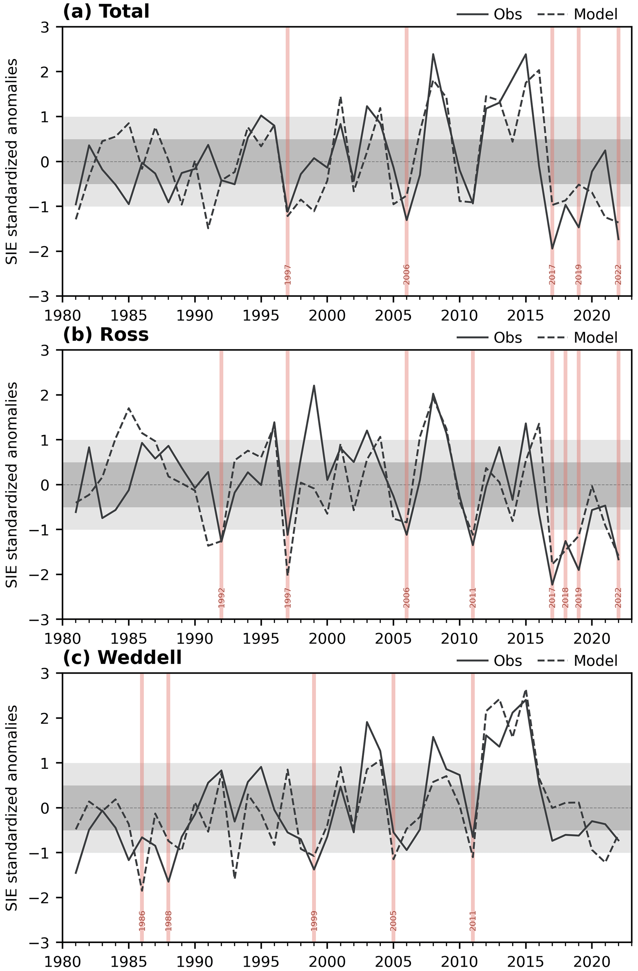
Figure 1 Standardized SIE anomalies in JFM computed over the total SO domain (a), the Ross region (b) and the Weddell region (c). Comparisons between the observations (obs; solid line) and model (dashed line) are shown. Dark- and light-grey shadings indicate ±0.5 and ±1σ, respectively. Years with a minimum SIE are marked in red.

3.2 Sea ice concentration

The related maps of observed JFM SIC anomalies during the five total minima and their composite are shown in Fig. 2. Negative anomalies, indicating an unusually low SIC, are mostly present in the Ross and Weddell sectors in all years, yielding a robust and significant signal in the composite map (Fig. 2f). However, the amplitude and location of the anomalies show some variability in both regions. In the Ross Sea, the negative anomalies in the three most recent years (Fig. 2c, d, e) are located near the coast and extend to most regions from 180 to 120° W, with values exceeding −0.5. In contrast, the remaining two years show a more complex structure, with mixed positive and negative anomalies (Fig. 2a, b). A more consistent signal is found in the Weddell Sea, with dipole-like anomalies that show an anomalous increase in SIC near the continent and an anomalous decrease at the sea ice edge over almost the entire sector; only 2022 stands out for the more westward location of the negative anomalies.

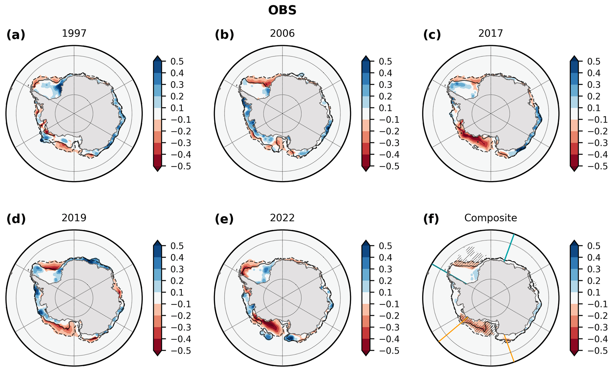
Figure 2 Shading: observed SIC anomalies in JFM in the years with total SIE minima (a–e) and their composite (f). Contours: sea ice edge (SIC = 0.15) in the respective years (solid line) and in the climatology (dashed line). Hatching in the composite map indicates statistically significant values, while the orange and green lines show the boundaries of the Ross and Weddell sectors, respectively.

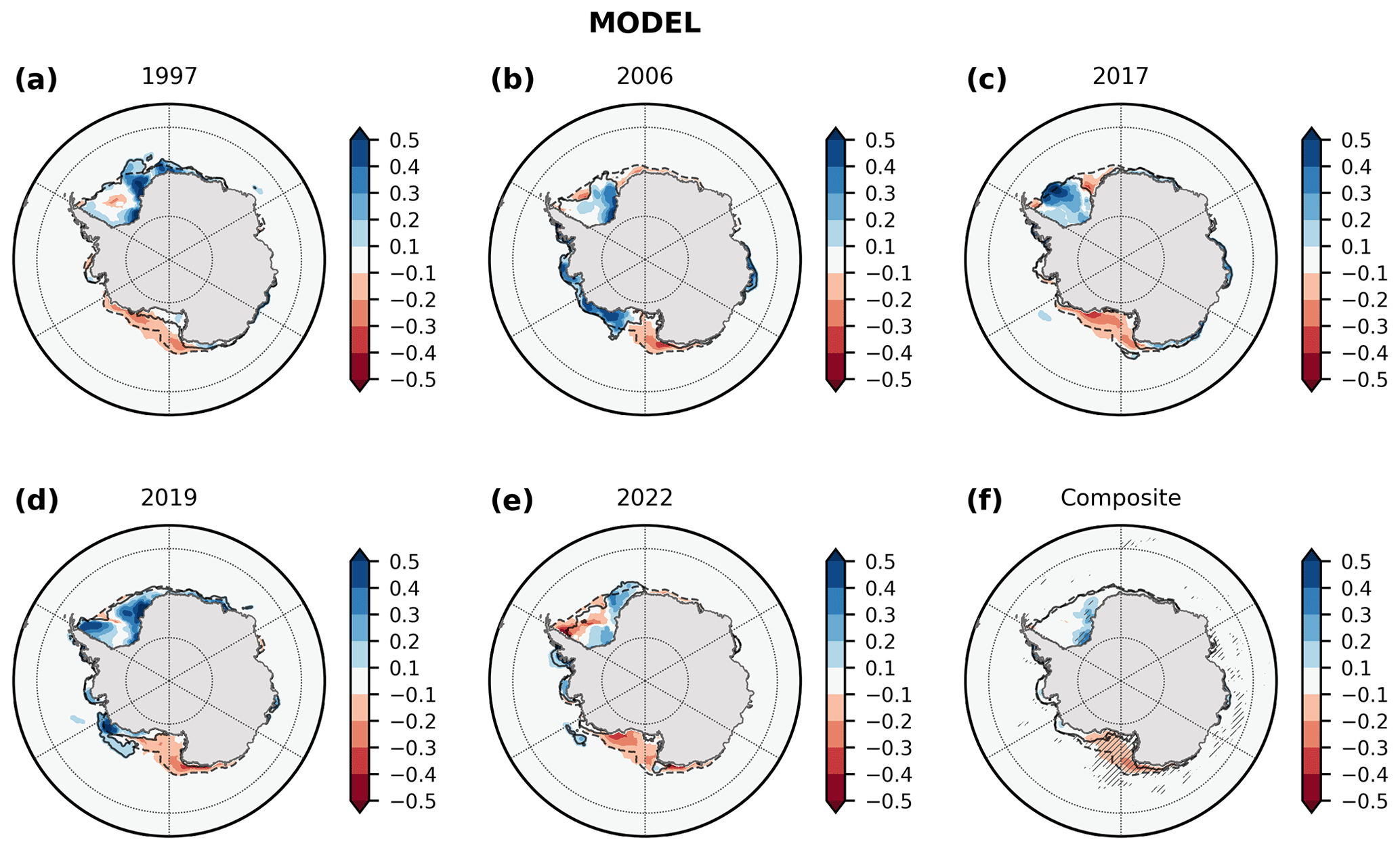
Figure 3 Same as Fig. 2 but for the model.

In the model, negative anomalies dominate in the Ross Sea and extend through the entire sector in 1997, 2017 and 2022 (Fig. 3a–d), while positive anomalies are also present in the region in 2006 and 2019. The resulting signal in the composite is a negative anomaly peaking west of 180°, in contrast with the observations, which tend to peak east of the dateline (compare Figs. 3f and 2f). This difference may be related to the model biases in the summer climatology discussed in Sect. 2, which result in limited sea ice left in the eastern Ross Sea in JFM (see Fig. S3). While the positive signal in the Weddell Sea that is evident in the observations is also reproduced by the model, only sparse negative anomalies are found in the model in the single years (Fig. 3a–e), and they are almost lacking in the composite map (Fig. 3f). Again, this may be related to the model's systematic summer biases. The observed negative anomalies in the western part of the sector are in fact located in regions where the model usually does not have sea ice at all (compare anomalies in Fig. 2 with the model's climatological sea ice edge in Fig. 3, dashed lines). In contrast, the lack of negative anomalies in the eastern part may be due to the model's tendency to overestimate the sea ice presence there, as discussed in Sect. 2 (see Fig. S2). The model also fails in reproducing the strength of the anomalies well, particularly for the 2017 and 2022 events. This may be also due to systematic biases in the model's mean state, which can affect the simulation of the anomalies: for example, a baseline mean sea ice state that is too thick in the model could explain that the summer sea ice area anomalies in a warm year are not as large as the observed ones.

Interestingly, years that are minima exclusively in the Weddell Sea show strong negative anomalies in the observations in that region, similar to the total case, but mostly positive ones in the Ross Sea, again confirming that the two sectors do not always contribute simultaneously to a total minimum (see Fig. S6). In contrast, turning to the Ross Sea regional minima, 1992 shows a similar pattern with anomalies of opposite sign in the two regions, while 2018 displays negative anomalies in both of them (Fig. S4). The year 2011, which is a regional minimum for both sectors, expectedly features a mixed signal (Fig. S4): as can be noted in the time series, it is very close to being defined as a total minimum (Fig. 1a), but positive anomalies in the Amundsen and East Antarctic sectors partially compensate for the negative ones in the Ross and Weddell seas. Though with different patterns and amplitudes, roughly similar results are found in the model (Figs. S5 and S7), except for 2005, which is a regional minimum in the Weddell Sea with pronounced negative anomalies in both sectors.

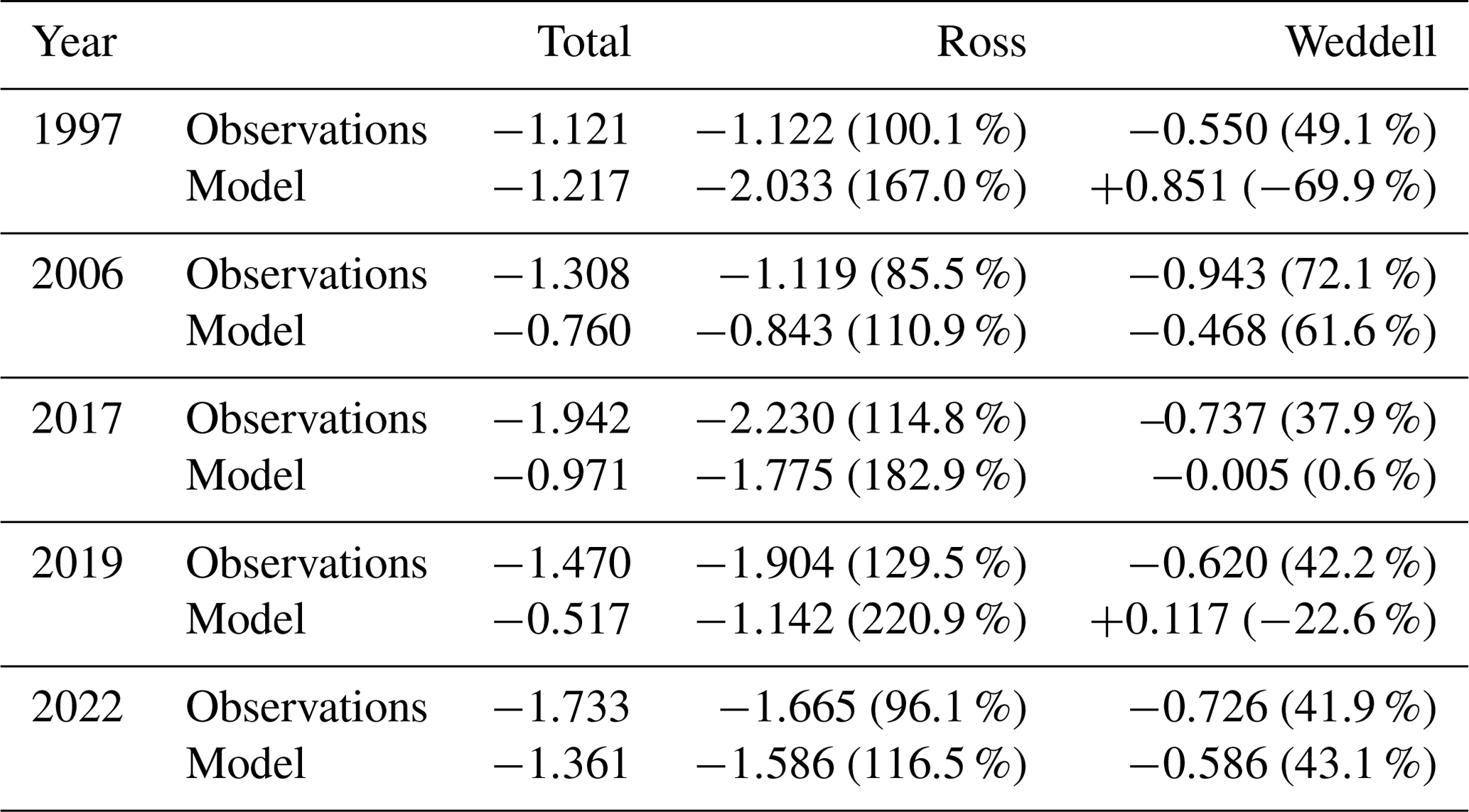
Overall, it emerges that the Weddell and Ross seas are the main regions contributing to the summer minima. Specifically, the Ross Sea's contribution to the total SIE anomalies (as in Fig. 1a) is about twice the one from the Weddell Sea in the observations (Table 1): on average, the Ross Sea accounts for around 105 % of the negative SIE anomalies, and the Weddell Sea accounts for around 49 % (note that their sum exceeds 100 % as other sectors contribute with positive anomalies). In the model, the Ross Sea's role is even larger (around 160 %), while the Weddell Sea's contribution is highly variable and typically underestimated. While the predominant role of these two regions is expected from the climatological distribution of sea ice, which tends to disappear in the other sectors during summer, it is interesting to note that the signal is clear and robust also in the composites. However, the two sectors behave independently, sometimes being even anti-correlated, with regional minima corresponding to regional high SIE in the other sector. In general, the Ross Sea shows a larger variability and a higher number of recorded minima, which often correspond to total ones. Furthermore, anomalies in the Weddell Sea tend to show a dipolar distribution with increased SIC next to the continent and decreased SIC at the sea ice margin.

Table 1 Standardized SIE anomalies in JFM (as in Fig. 1) during the years selected as circumpolar minima in the observations and model. The values refer to the SIE computed over the entire Southern Ocean domain (Total) and over the Ross and Weddell sectors in the respective columns. The percentages in parenthesis indicate the relative contribution of the two sectors to the total (negative) anomalies. Note that, for a certain year, the sum of the two percentages can exceed 100 % due to the positive contributions from other sectors.

3.3 Role of winter sea ice extent

So far, we have focused on summer and based our definition of the minima on SIE anomalies in JFM, since this season also corresponds to the minimum in the climatological seasonal cycle of sea ice extent. However, one may wonder whether these summer minima are preceded by anomalous sea ice conditions during the previous seasons, as discussed in several predictability studies (e.g., Holland et al., 2013; Marchi et al., 2018; Ordoñez et al., 2018; Libera et al., 2022). In particular, negative SIE anomalies already in winter would correspond to less sea ice to melt during the following months and could hence favor the summer minima.

To explore this hypothesis, we considered monthly standardized SIE anomalies ranging from the preceding September, i.e., when the annual maximum is reached at the end of winter, to March. In the observations, negative anomalies of the total SIE extent (Fig. 4a) start to appear already in September and are maintained until March for the last three years (2017, 2019 and 2022), while 1997 displays a mixed behavior and 2006 only shows signs of an incoming minimum from December onwards.

The observations thus suggest a role of winter preconditioning at least during the most recent years, but the model is not able to reproduce this behavior, since clear negative anomalies during all seven months are seen in 2022 only (Fig. 4d).

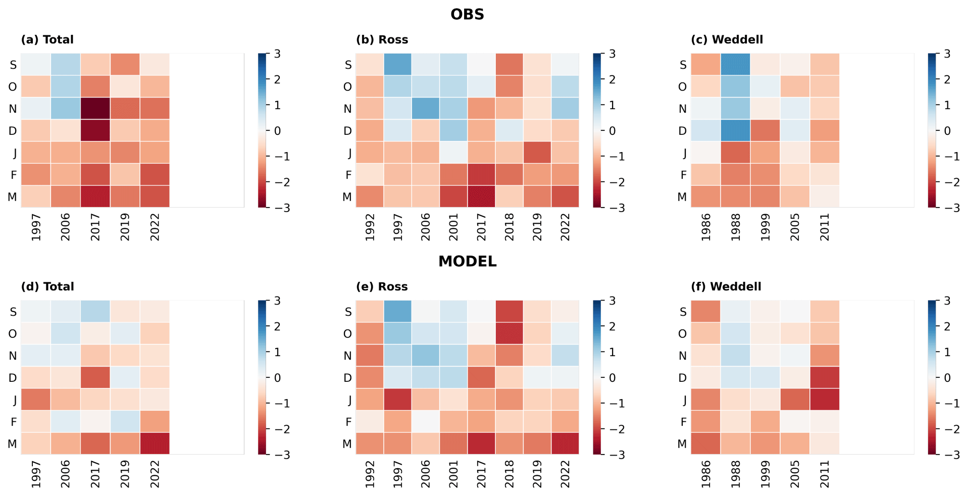
Figure 4 Monthly standardized SIE anomalies in the observations (a–c) and model (d–f) for the years with summer SIE minima, starting from the previous September. SIE computed over the total SO domain (a, d), the Ross region (b, e) and the Weddell region (c, f).

This is further supported by Hovmöller diagrams displaying time–longitude sea ice area anomalies for the five total minima (Figs. S8, S9), helping to identify the potential propagation of winter anomalies between different sectors. However, there is no consistent zonal migration of negative anomalies from one sector to another, leading to the sea ice minima. We also do not observe any clear sign of winter preconditioning in the earlier years (1997, 2006) and in the composites, particularly in the model (panels a, b, f of Figs. S8 and S9). It is only in some of the most recent cases (2017, 2019 and 2022) that persistent negative anomalies from at least the previous September are present in the Weddell and Ross sectors (panels c, d, e of Figs. S8 and S9).

The results for the regional minima in the Weddell and Ross sectors (Fig. 4, center and right columns) also do not support a straightforward link between winter and summer anomalies. In contrast to the total SIE, the results are very similar in the model and the observations for each region. Some years show indeed consistent negative anomalies through most of the warm season (1992, 2018, 2019 in the Ross Sea; 1999 and 2011 in the Weddell Sea) so that the influence of the winter sea ice state cannot be excluded, but it is not the case in many other years. Overall, our results indicate a marginal role of a reduced winter extent in preconditioning a summer minimum.

3.4 Atmospheric circulation and surface winds

Different processes may contribute to the anomalous melting of sea ice resulting in a SIE minimum. Since winds strongly influence sea ice through both heat advection and mechanical transport, anomalous conditions in the atmospheric circulation during the preceding months could drive the summer SIE events (Holland and Kwok, 2012; Kusahara et al., 2019). Hence, in this section, we examine sea level pressure (SLP) and 10 m wind anomalies during the previous season (OND, October–December) that lead to minimum sea ice extent in summer. The importance of atmospheric spring conditions for the summer and autumn sea ice state has been shown in several studies (e.g., Holland et al., 2017; 2018), and previous works examining the 2017 and 2022 minima also considered this season (e.g., Purich and England, 2019; Yadav et al., 2022). Furthermore, as seen in the previous section, the sea ice anomalous conditions are already set up in January at the latest, indicating the important role of surface winds during the previous months.

Anomalous maps of SLP and winds for the total minima are shown in Fig. 5 (similarly to Figs. 2 and 3): note that they are the same for the reanalysis and the model, since the latter is forced by the same atmospheric fields (see Sect. 2). Anomalous SLP centers are present in the Bellingshausen–Amundsen sector during most years, which is consistent with a role of the ASL. However, the ASL is sometimes strengthened (1997, 2022; Fig. 5a, e) and sometimes weakened (2006, 2017; Fig. 5b, c). A deepened ASL emerges in the composite (Fig. 5f), but this signal is likely dominated by 2022, which shows strong anomalies beyond −10 hPa (Fig. 5e). Mixed conditions also emerge for the SAM, with some years characterized by more westerly winds (1997, 2019, 2022) and others in which the westerly winds are weaker. Similarly, the corresponding patterns for the regional minima in the Weddell and Ross sectors are quite diverse and do not provide a clear indication of a preferred status of the ASL or other large-scale features in the months prior to a SIE summer minimum (Figs. S10 and S11).

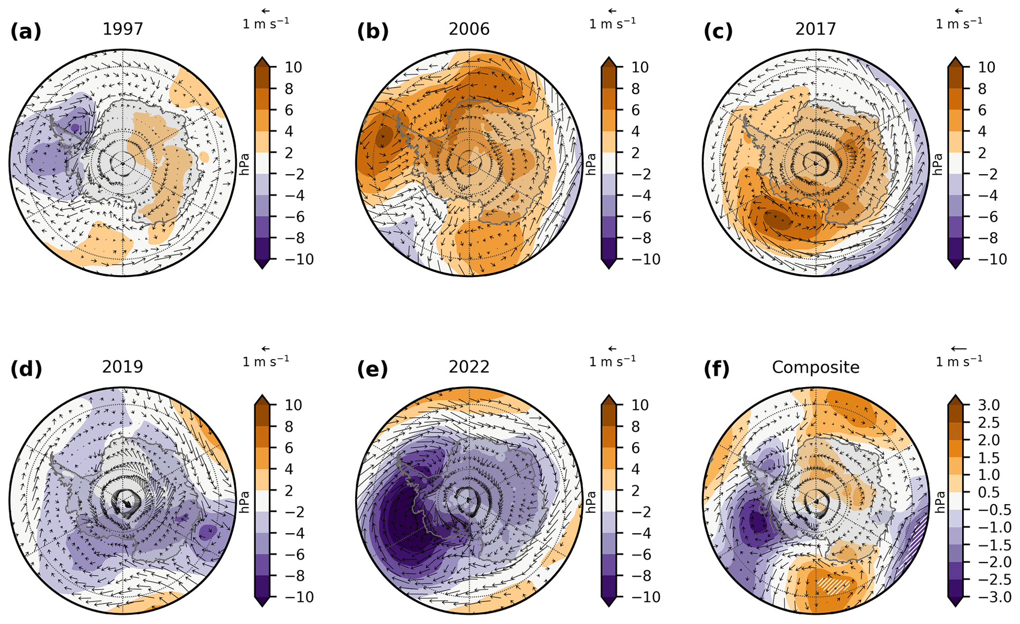
Figure 5 SLP (shading) and 10 m wind (arrows) anomalies in the years with total SIE minima (a–e) and their composite (f) during the previous spring (OND). Hatching in the composite map indicates statistically significant SLP values.

Even if they might emerge from different large-scale patterns, the anomalous low-level winds exhibit at least a dominant direction in the two key sectors (Ross and Weddell) for most of the years, roughly corresponding to the direction appearing in the composite. We confirm and quantify this by computing the average wind direction in the Weddell and Ross sectors (as defined in Sect. 2.2) over the grid points with negative JFM SIC anomalies greater than −0.1 (namely, areas with red shading in Figs. 2 and 3). Note that, in this case, different values for the observations and model are shown, since the SIC anomalies are distinct. The results for all the years, including total and regional minima, are reported in Fig. 6 in terms of wind angle with respect to the zonal direction: an angle of 0° (180°) represents pure westerly (easterly) winds, and a value of 90° (270°) indicates a pure southerly (northerly) component. Most points are found in the first and fourth quadrants, indicating that the anomalous winds during these years are predominantly westerly but have varying meridional components. In the Ross region (orange points) the values are confined to a small range, being mostly found between around 310 and 60°, which suggests a prevailing westerly–southwesterly component, in agreement with Holland et al. (2017). In contrast, a larger spread is observed concerning the Weddell sector (green points), but approximately two-thirds of the points are found in the fourth quadrant, indicating a dominant northwesterly component. A notable exception is 2017, particularly in the observations, with a mostly southerly component in the Weddell Sea, as seen in Fig. 5c. Though it is challenging to identify common large-scale circulation anomalies, these results show that the regional wind conditions in the Ross and Weddell sectors share some similarities across the minima. The dominant northwesterly anomalous winds in the Weddell Sea are consistent with the dipolar distribution of SIC, with warm air coming in from lower latitudes, pushing the sea ice towards the coasts of Antarctica (Figs. 2f, 3f and 5f). The prevailing southwesterly anomalous flow in the Ross Sea, in contrast, suggests winds mainly coming from the continent and transporting the sea ice away. The exact roles of dynamics and thermodynamics in leading the summer SIC anomalies are examined in more details in the next section, for both regions.

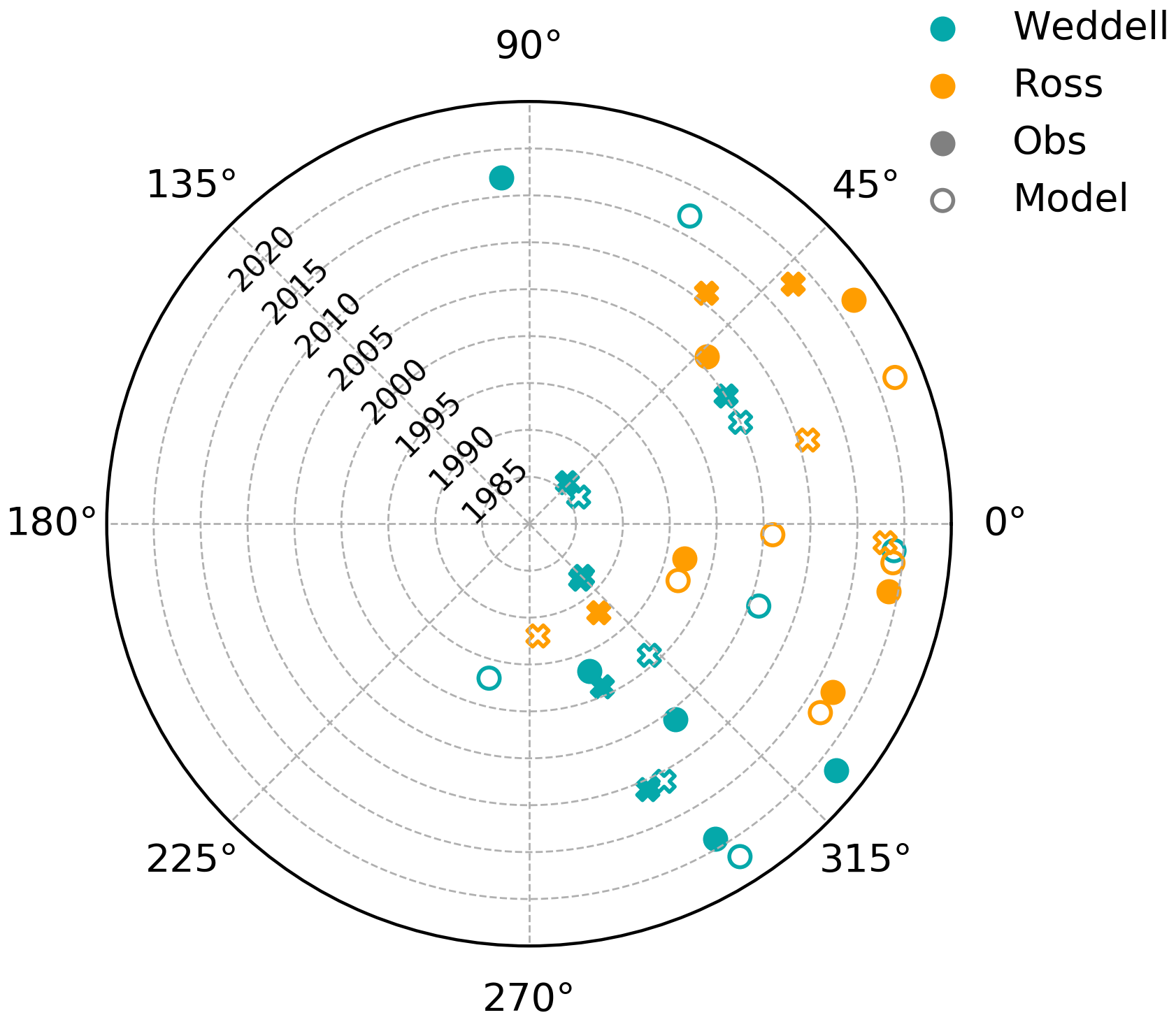
Figure 6 Average OND 10 m wind direction for all extreme years in the observations (filled points) and model (empty points). Circles indicate years with total minima, while crosses are for years with regional minima. The values indicate the angle of the wind vectors with respect to the zonal axis: 0° for pure westerly, 90° for pure southerly, 180° for pure easterly and 270° for pure northerly winds. See the main text for details.

3.5 Sea ice concentration budget

We have shown that the exceptional sea ice melting during the minima is related to anomalous surface winds that share some common regional features throughout most of the events. However, the fundamental mechanisms governing this exceptional reduction have not been examined yet, as well as, in particular, the contribution of dynamic and thermodynamic processes. To assess this, we used the model diagnostics for the budget described in Sect. 2.3. We computed the anomalous values of the dynamic and thermodynamic terms for the minima over November–January (NDJ) to encompass the sea ice evolution during the two seasons examined above (OND and JFM) but focusing on the melting season for consistent anomalies (see the monthly climatologies in Figs. S12–14).

Note that the dynamic and thermodynamic terms are not mutually independent as they influence one another both directly and indirectly and it is not possible to strictly separate them. For instance, an anomalous transport of sea ice away from a given point, thus driven by dynamics, would be compensated by opposite anomalies in the thermodynamic term as less sea ice becomes available for melting. In turn, leads created by sea ice transport, effectively a dynamic process, induce ocean warming and melting associated with the albedo–temperature feedback (e.g., Goosse et al., 2023), which is the dominant mechanism in spring. However, this melting is accounted for in the thermodynamic part in the framework proposed here, and the information about the role of dynamics is not explicitly retained. Hence, the thermodynamic and dynamic terms must be interpreted carefully, particularly the modulation of the thermodynamic component by its dynamic counterpart, which includes not only direct compensation of the anomalies but also more complex feedback mechanisms. With this in mind, it is not surprising to see that, locally, both terms contribute to the anomalous sea ice loss during the months preceding a summer minimum (Fig. S15). In fact, the negative tendency anomalies in the inner Ross and Weddell seas arise from the combined influence of dynamic and thermodynamic processes, which have comparable strength at the local scale as they sustain one another.

While it is evident that both terms play a role, a clear interpretation and quantification of their contributions is not straightforward from the spatial patterns, as they are quite heterogeneous (Fig. S15). For this reason, we have averaged the NDJ anomalies of the dynamic and thermodynamic terms over areas in the Weddell and Ross sectors with negative JFM SIC anomalies ($<-\mathrm{0.1}$), similarly to Fig. 6. The results reported in Fig. 7 thus represent the mean relative contribution of the two components to the total SIC change in these regions, for all years (total and regional minima). In both sectors, most years present negative values for the two terms, indicating that both types of processes tend to lead to direct sea ice loss. For instance, surface winds may transport sea ice away while also advecting warm air towards a region, which in turn increases the ocean–sea ice heat flux and favors basal melting. Direct surface melting from thermal advection is supposed to play a minor role in spring, but it may be overestimated in our model (Fig. S16). In a few years, such as 1997 in the Ross Sea (top), 2017 in the Weddell Sea (bottom) and 2007 in both regions, a moderate positive contribution from the dynamics is present, suggesting that more sea ice is transported mechanically to the area only for it to rapidly melt (negative thermodynamic term), again yielding an overall negative anomalous tendency. The prevailing southerly wind direction in the Weddell sector in 2017 is indeed different than in the rest of the years (see Fig. 6) and consistent with exceptional ice convergence and melting in the northeastern part of the basin (compare Figs. 2c and 3c). In this framework of spatial averages, the thermodynamic term typically exceeds, in absolute value, its dynamic counterpart, suggesting a predominant but not exclusive role of thermodynamics over dynamics. Some notable exceptions are however present: in 2022, dynamics leads in both sectors, as in 2011 and 2017 in the Weddell region. The thermodynamic term is mostly negative, and its range is similar in the two sectors: from −1.317 to $-\mathrm{0.140}\times {\mathrm{10}}^{-\mathrm{3}}$ d⁻¹ in the Ross Sea and between −1.143 to $\mathrm{0.066}\times {\mathrm{10}}^{-\mathrm{3}}$ d⁻¹ in the Weddell Sea. In contrast, the dynamic term spans both positive and negative values, between −0.558 and $\mathrm{0.336}\times {\mathrm{10}}^{-\mathrm{3}}$ d⁻¹ in the Ross Sea and ranging from −1.908 to $\mathrm{1.168}\times {\mathrm{10}}^{-\mathrm{3}}$ d⁻¹ in the Weddell Sea, confirming that the two terms can be comparable in some cases, particularly in the Weddell sector.

This analysis of the spatially averaged budget has allowed us to quantify the contributions of these processes at the large, regional scale and suggests a more prominent role of thermodynamics. However, we stress that the movement of ice away and from adjacent points inside the sector is largely balanced in such spatial averages. Hence, the resulting (anomalous) dynamic term accounts for the net ice transport in or out of the region but does not consider the local contributions that, as seen above, are comparable to the thermodynamic processes and can in fact modulate them.

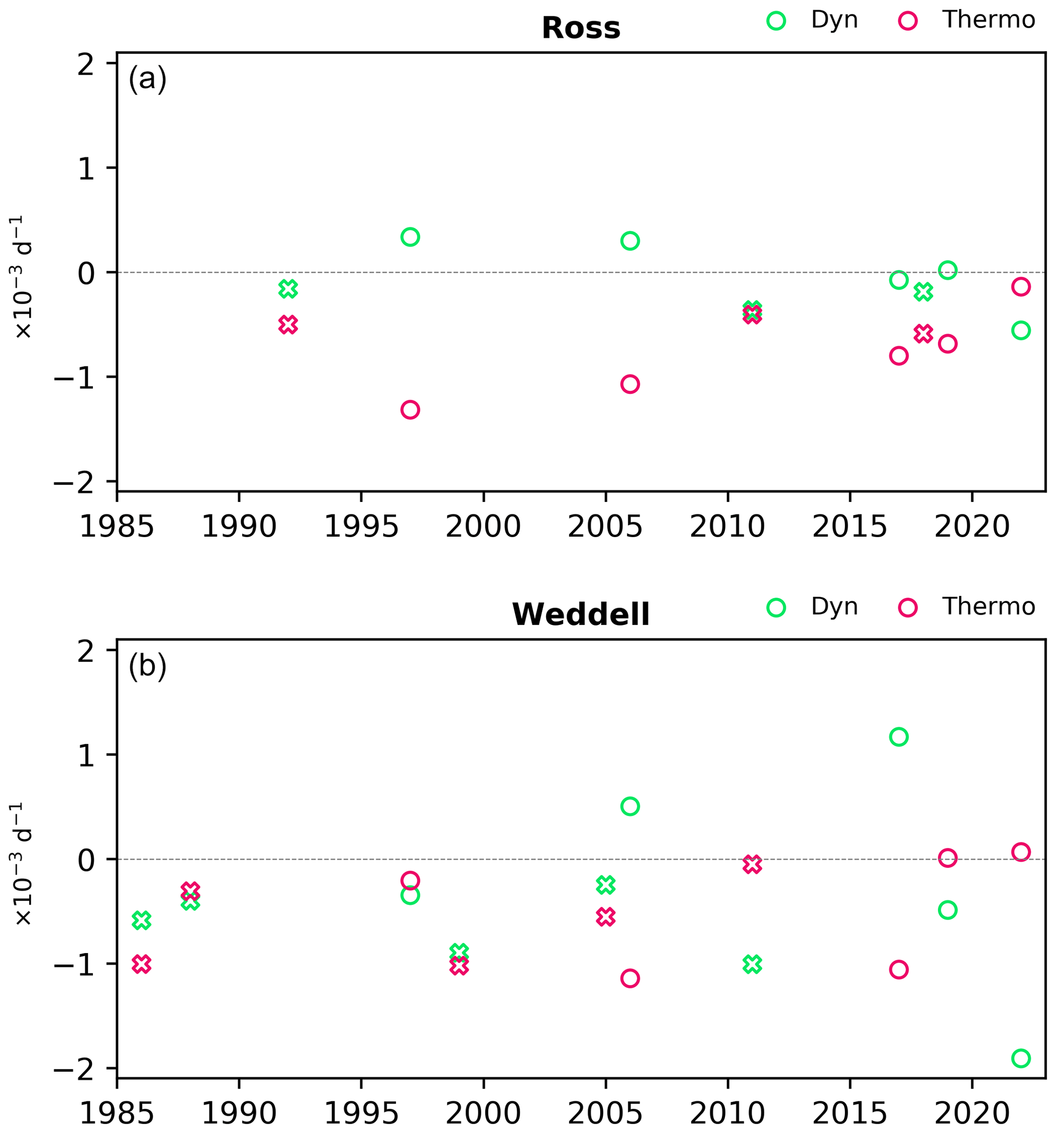
Figure 7 Average anomalous dynamic (green) and thermodynamic (magenta) contributions to the sea ice budget in NDJ for the Ross (a) and Weddell (b) regions. Circles indicate years with total minima, while crosses are for years with regional minima. See the main text for details.

4 Discussion and conclusions

We have examined sea ice and atmospheric conditions before and during summer SIE minima over the satellite period up to 2022, in observations and in a regional ocean–sea ice model driven by atmospheric fields from ERA5. We have highlighted that the sectors mainly contributing to circumpolar minima are the Weddell and Ross seas, in agreement with previous studies for 2017 (e.g., Turner et al., 2017) and 2022 (e.g., Wang et al., 2022) and consistent with the summer climatological conditions, which feature little sea ice in the other sectors. However, we have also highlighted regional differences: the Ross Sea experiences a higher number of recorded minima, which often correspond to total ones; in turn, regional minima in the Weddell Sea are usually balanced by excess of sea ice in the other sectors. Hence, our results indicate that the variability of the Ross Sea leads the minima, even though the synergy with the Weddell Sea was crucial in the latest cases (2017, 2019, 2022). These results are consistent with previous reports of strong regional differences in the inter-annual and long-term variability of Antarctic sea ice (e.g., Zwally et al., 2022; Parkinson and Cavalieri, 2012; Comiso et al., 2017) but are here applied to SIE minima for the first time.

We have also shown that, during these events, SIC anomalies in the Weddell Sea tend to present a dipolar distribution, with anomalous ice accumulation towards the continent, while the Ross Sea tends to have a more homogenous decrease. This further stresses the regional differences and suggests distinct mechanisms at play in the two sectors. To investigate these mechanisms, we have tested various processes potentially contributing to the development of the summer SIE minima: the role of wintertime sea ice conditions prior to the minima, the impact of the anomalous springtime winds, and the contribution of dynamics and thermodynamics to the exceptional sea ice loss.

First, we have explored the hypothesis that the summer minima are preceded by anomalous sea ice conditions already in winter and are hence a consequence of less sea ice being available for melting in the first place. However, by examining monthly SIE anomalies from the previous September, we have not found a clear and consistent role of the wintertime sea ice preconditioning. In fact, this contribution is minor in most years before 2017, indicating that those minima are mainly driven by atmospheric conditions. However, a more prominent role emerges for the last events (2017, 2019, 2022). Substantial uncertainty remains, and more data from the next years are needed to understand if it is accidental or if new patterns are emerging.

Next, considering the prominent impact of winds on sea ice variability (Holland and Kwok, 2012; Hobbs et al., 2016; Kusahara et al., 2019), we have examined the role of surface atmospheric circulation anomalies during the previous spring in driving the summer SIE minima. Surface winds and hence sea ice can be modulated by typical modes of atmospheric variability such as the El Niño–Southern Oscillation (ENSO); the SAM; the ZW3 pattern; the Indian Ocean Dipole; and other remote forcings, for instance from the stratosphere (e.g., Turner, 2004; Raphael, 2007; Thompson et al., 2015). In particular, the 2022 minimum has been attributed to the combined effects of La Niña and a positive SAM, which both contributed to strengthening the ASL (e.g., Turner et al., 2022). Several studies have suggested an impact of ENSO on the atmospheric circulation at southern high latitudes, mostly related to the poleward propagation of an anomalous Rossby wave train at upper levels (e.g., Turner, 2004; Li et al., 2021; Lee and Jin, 2023). A prominent feature of this teleconnection is a weakened (strengthened) ASL during El Niño (La Niña) events, which could in turn affect sea ice in the adjacent regions. However, the atmospheric response is highly variable between ENSO events and likely modulated by the phase of the SAM (e.g., Hobbs et al., 2016). Hence, the impact of ENSO on Antarctic sea ice is even harder to establish (Simpkins et al., 2012). Simple linear regressions of SIC anomalies on the Niño 3.4 index suggest that anomalous sea ice loss is associated with El Niño in the Ross sector and with La Niña in the Weddell sector, in spring and more weakly in summer (Fig. S17). The summer SIE minima examined here could thus encompass a contribution from ENSO variability, but a clear role is difficult to identify as no preferred ENSO phase emerges in our sample (Fig. S18): the five years considered total minima follow different ENSO phases (El Niño in 2019, neutral conditions in 1997 and 2019, La Niña in 2006 and 2022).

Our analysis does not identify a clear unique large-scale atmospheric mode as the driver of the summer SIE minima, though we acknowledge the potential impact of the superposition of different modes. More generally, there is not a clear anomalous atmospheric pattern emerging as a common feature to all or most minima, such as a preferred status of the ASL. Instead, the large-scale circulation is more related to the specific events, with anomalous SLP centers of action in distinct locations depending on the case. However, we argue that different large-scale anomalies in the atmospheric circulation can nonetheless lead to similar regional prevailing winds, which ultimately influence the sea ice variability. Specifically, our results indicate that SIE minima are associated with dominant northwesterly anomalous winds in the Weddell Sea and a prevailing southwesterly anomalous flow in the Ross Sea. These local atmospheric conditions seem to be the main common driver of most summer SIE extremes. We remark that our analysis, which is based on seasonal means, does not explicitly address the possible role of individual storms, which has been suggested to be relevant contributors to, at least, the 2022 minimum (e.g., Turner et al., 2022).

Finally, we investigated whether the anomalous sea ice loss leading to a summer SIE minimum is mostly driven by dynamic processes, such as sea ice motion and mechanical redistribution, or thermodynamic contributions, such as the melting of sea ice in open water or local vertical processes. The regional differences concerning the predominant winds could suggest distinct contributions from dynamics and thermodynamics in the Ross and Weddell seas; however, our results are similar for the two regions. We find that, locally, both terms are important and affect sea ice both directly, via mechanical transport and thermal melting, and indirectly, through feedback mechanisms. At the larger, regional scale, we observe that the exceptional sea ice loss in both sectors is generally dominated by thermodynamic processes, though dynamics also play a role, albeit minor. These results are consistent with the estimate of Wang et al. (2022) for the 2022 event, for which they found that both terms contribute in spring to the anomalous sea ice loss, and with Kusahara et al. (2018), who demonstrated the prevalence of thermodynamic forcings for the spring extreme in 2016, ahead of the summer 2017 minimum. Both types of contributions are influenced by the winds, which transport warm and cold air masses, as well as the sea ice itself, along with other processes.

Note that alternative selection criteria for the minima could be used. For instance, Turner et al. (2020) simply considered the lower quartile of sea ice annual minimum extents. The method does not strongly affect the final collection of years in the observations, where the total minima could be identified almost by eye (Fig. 1a), but in our case it is relevant for the comparison with the model. We have tested various criteria, such as different thresholds or the selection of distinct years for the observations and the model, but they typically lead to samples that are too small or inconsistent, since the model sometimes simulates SIE minima that are not observed and vice versa. The final selection of events is based on concurrent conditions for both the observed and modeled time series to ensure the analysis of a reasonable number of observed events that are also captured by the model.

We finally remark that the model's results must be interpreted within the simulation biases and limitations. For instance, the experimental setup with imposed atmospheric conditions does not permit estimating the influence of the ocean–sea ice system on the atmosphere and consequent feedbacks, which likely play a role in the occurrence of minima (e.g., Goosse et al., 2023). We have also discussed the model's biased climatology and how it is related to the model's poor performance in capturing the exact distribution of SIC anomalies, particularly in the Weddell Sea. Nevertheless, the main processes explaining the occurrence of minima in the model are consistent with the ones derived from observations, and thus both support our conclusions. Our budget analysis relies on the model only and is thus affected by its biases, such as the overestimated surface melting in the Weddell Sea mentioned in Sect. 3.5. Furthermore, the underestimation of the negative anomalies at the sea ice edge in the Weddell Sea could also impact the budget and alter the role of ice transport. However, the overall results are consistent between the Ross Sea and Weddell sectors and in agreement with previous results, as discussed above, which further endorses our conclusions.

After the 2022 minimum, a new record was established in summer 2023 (Liu et al., 2023; Purich and Doddridge, 2023), which we have not included in the study due to data unavailability at the time of the analysis. The distribution of SIC anomalies was in line with the previous events, with prominent negative anomalies in the Weddell and Ross seas. However, a substantial lack of sea ice was observed in all sectors and particularly in the Bellingshausen Sea–Amundsen sector (Fig. S19). The atmospheric conditions during the previous spring were again dominated by a positive SAM. In addition to a deepened ASL, similarly to 2022, a cyclonic anomaly appeared over the eastern Weddell sector (Fig. S20). This anomalous large-scale circulation led to prevailing westerly winds, in agreement with the previous cases, though an unusual southerly component was present in the Weddell Sea. While these results are consistent with our main findings for the other events, we speculate that preconditioning played a more important role in 2023 than in other years. In fact, sea ice never fully recovered after the 2022 minimum, and negative SIE anomalies persisted even after the annual winter peak, which might have favored the occurrence of the subsequent summer minimum.

Currently, as we approach the end of the 2023 growth season and Antarctic sea ice is supposed to reach its maximum annual extent, unprecedented anomalies are still occurring. It is probable that a new record will be established, raising more concerns about the future of Antarctic climate. With this work, we contribute to understanding the main process of driving these extreme events as we wait for the likely next record to see how it will fit with our conclusions.