Post-depositional modification on seasonal-to-interannual timescales alters the deuterium-excess signals in summer snow layers in Greenland

We document the isotopic evolution of near-surface snow at the East Greenland Ice Core Project (EastGRIP) ice core site in northeast Greenland using a time-resolved array of 1 m deep isotope (δ¹⁸O, δD) profiles. The snow profiles were taken from May–August during the 2017–2019 summer seasons. An age–depth model was developed and applied to each profile, mitigating the impacts of stratigraphic noise on isotope signals. Significant changes in deuterium excess (d) are observed in surface snow and near-surface snow as the snow ages. Decreases in d of up to 5 ‰ occur during summer seasons after deposition during two of the three summer seasons observed. The d always experiences a 3 ‰–5 ‰ increase after aging 1 year in the snow due to a broadening of the autumn d maximum. Models of idealized scenarios coupled with prior work indicate that the summertime post-depositional changes in d (Δd) can be explained by a combination of surface sublimation, forced ventilation of the near-surface snow down to 20–30 cm, and isotope-gradient-driven diffusion throughout the column. The interannual Δd is also partly explained with isotope-gradient-driven diffusion, but other mechanisms are at work that leave a bias in the d record. Thus, d does not just carry information about source-region conditions and transport history as is commonly assumed, but also integrates local conditions into summer snow layers as the snow ages through metamorphic processes. Finally, we observe a dramatic increase in the seasonal isotope-to-temperature sensitivity, which can be explained solely by isotope-gradient-driven diffusion. Our results are dependent on the site characteristics (e.g., wind, temperature, accumulation rate, snow properties) but indicate that more process-based research is necessary to understand water isotopes as climate proxies. Recommendations for monitoring and physical modeling are given, with special attention to the d parameter.

1 Introduction

The relative concentration of stable water isotopes in polar snow and ice has proven useful in temperature reconstructions of Earth's climate (e.g., Lorius et al., 1990; Jouzel et al., 1997, 2003; Johnsen et al., 2001; Kavanaugh and Cuffey, 2003; Steig et al., 2013). In the past, these reconstructions were dependent on understanding the sensitivity of changes in water isotopes in polar snow and ice to changes in mean annual temperature in the polar regions, i.e., the water-isotope–temperature sensitivity. Small changes in this sensitivity have significant influence on inferences about past climates based on water isotope records from polar ice cores (e.g., Grootes et al., 1993; Charles et al., 1994; Petit et al., 1999; Jouzel et al., 2003). Recent climate reconstruction efforts are not as dependent on temperatures inferred from water isotopes in polar snow because they use other proxies to understand regions outside of the poles (e.g., Rohling et al., 2012; Dahl-Jensen et al., 2013; Buizert et al., 2021). Simulations of past polar ice sheet mass balance and climate still require accurate knowledge of ice sheet temperatures often derived from empirical isotope–temperature sensitivities (e.g., Cuffey et al., 2016; Jones et al., 2023) or more nuanced meteorological approaches involving regional temperature gradients and patterns in air mass transport (e.g., Markle and Steig, 2022). Inferences about past circulation and weather patterns are also possible from combinations of isotope and other chemistry measurements from polar snow and ice (e.g., Mayewski et al., 1994; Steffensen et al., 2008; Guillevic et al., 2013; Jones et al., 2018). Such understanding is important not only to make claims about past climate, but to improve models for prediction of weather and future climate (e.g., Blossey et al., 2010; Werner et al., 2011; Dee et al., 2015; Dütsch et al., 2019).

Despite the importance of isotope signals in polar snow and ice to understanding climate and temperature, there remains a lack of contiguous understanding of the integrated relationship between local and regional climate and the isotopic composition of polar snow from water source to eventual extraction. Specifically, there is uncertainty about what happens to the isotopic signal in the top meter of snow when it is still under the influence of local meteorology. This study provides observations of meteorology-induced isotopic changes in surface and near-surface snow. Subsequent analysis and modeling provoke some revised interpretation of the d climate proxy.

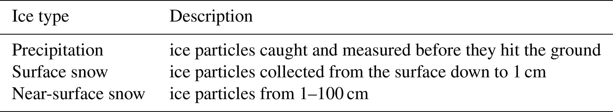
Table 1 Terms used in this study to describe different sources of solid water isotope.

1.1 Water isotopes in the atmospheric hydrologic cycle

The part of the global hydrologic cycle that brings precipitation to the polar regions provides several opportunities for isotopic fractionation. The relative isotopic content of the precipitation (Eq. 1) is therefore thought to represent an integrated history of the water from source to sink (Craig, 1961; Dansgaard, 1964; Gonfiantini, 1978). It is important to clarify here that the prior literature relating to water isotopes in polar snow and ice often uses the terms precipitation, surface snow, and near-surface snow interchangeably. Our thesis requires us to keep these terms distinct; our usage is outlined in Table 1. We apply these same terms to the past literature no matter what term was used in the original literature.

$$\begin{array}{}\text{(1)}& {\mathit{\delta }}^{\mathrm{18}}\mathrm{O}=\left({\displaystyle \frac{{\frac{{\mathrm{H}}_{\mathrm{2}}^{\mathrm{18}}\mathrm{O}}{{\mathrm{H}}_{\mathrm{2}}^{\mathrm{16}}\mathrm{O}}}_{\text{sample}}}{{\frac{{\mathrm{H}}_{\mathrm{2}}^{\mathrm{18}}\mathrm{O}}{{\mathrm{H}}_{\mathrm{2}}^{\mathrm{16}}\mathrm{O}}}_{\text{standard}}}}-\mathrm{1}\right)\end{array}$$

Water isotopes in the global hydrologic cycle have been monitored extensively since the 1960s, illustrating robust linear relationships between δ¹⁸O and δD (Eq. 2). The y intercept of this relationship is commonly referred to as “deuterium excess” (d-excess or d; Eq. 3; e.g., Dansgaard, 1964; Merlivat and Jouzel, 1979; Jouzel and Merlivat, 1984). A mean d value of approximately 10 ‰ for global precipitation is thought to represent equilibrium fractionation conditions (Dansgaard, 1964). The d parameter is often used as an integrated characterization of an air mass's hydrologic source and transport history (Merlivat and Jouzel, 1979; Jouzel and Merlivat, 1984; Ciais and Jouzel, 1994; Pfahl and Sodemann, 2014; Hu et al., 2022). The mean Northern Hemisphere d seasonal cycle has a maximum in winter and minimum in summer from hemispherically averaged Global Network of Isotopes in Precipitation stations (Pfahl and Sodemann, 2014). However, Johnsen and White (1989) observed an autumn peak and spring minimum in d from near-surface snow. Kopec et al. (2022) recently observed a summertime peak in d in precipitation at Summit, Greenland, possibly shifted from autumn due to the influence of upwind sublimation from the ice sheet. Similar discrepancies exist in Antarctic records. Delmotte et al. (2000) show a d seasonal cycle in shallow cores from the coastal Law Dome site in East Antarctica that peaks in winter and has a minimum in the autumn and summer. However, Schlosser et al. (2008) show a more complicated d signal exists when considering snow with minimal exposure to post-depositional effects. Through back trajectory compositing, they show that moisture with an oceanic origin has a maximum d in winter and a minimum in summer.

$$\begin{array}{}\text{(2)}& {\displaystyle }& {\displaystyle }\mathit{\delta }\mathrm{D}=\mathrm{8}\cdot {\mathit{\delta }}^{\mathrm{18}}\mathrm{O}+\mathrm{10}\text{(3)}& {\displaystyle }& {\displaystyle }d=\mathit{\delta }\mathrm{D}-\mathrm{8}\cdot {\mathit{\delta }}^{\mathrm{18}}\mathrm{O}\end{array}$$

Linear relationships between mean annual air temperature and water from precipitation or near-surface snow (a.k.a. isotope–temperature sensitivity) have also been defined using spatially distributed measurements (γ_s; see Eq. 4; Dansgaard, 1964). Often different linear relationships exist for similar areas when looking at temporally oriented data sets and models (γ_t; e.g., Cuffey et al., 1995, 2016; Werner et al., 2018).

$$\begin{array}{}\text{(4)}& {\mathit{\gamma }}_{\mathrm{s},\mathrm{t}}={\displaystyle \frac{\mathrm{\Delta }{{\mathit{\delta }}^{\mathrm{18}}\mathrm{O}}_{\mathrm{s},\mathrm{t}}}{\mathrm{\Delta }{T}_{\mathrm{s},\mathrm{t}}}}\end{array}$$

Improved modeling of the hydrologic cycle and cloud physics is a primary focus of current isotope-enabled models (IEMs) with a range of complexity, which has improved interpretation of snow and ice cores (e.g., Merlivat and Jouzel, 1979; Jouzel and Merlivat, 1984; Johnsen and White, 1989; Ciais and Jouzel, 1994; Blossey et al., 2010; Werner et al., 2011; Markle and Steig, 2022). Some focus is still on water-isotope–temperature relationships like γ_t (e.g., Werner et al., 2018). Yet, it is recognized that a more comprehensive, process-based approach to isotope–climate relationships using trajectory mixing, source-to-sink temperature gradients, and nonlinear isotope-to-temperature sensitivities is necessary due to the complexity of integrated processes leading up to deposition (e.g., Markle and Steig, 2022).

A challenge for all climate-to-isotope relationships and IEMs is validation. These relationships and IEMs are compared, or even tuned, to surface and near-surface snow that was treated as precipitation (e.g., Jouzel and Merlivat, 1984; Johnsen and White, 1989; Petit et al., 1991; Uemura et al., 2012; Werner et al., 2018; Dütsch et al., 2019; Markle and Steig, 2022). However, the snow will have spent months or years exposed meteorologically influenced post-depositional processes. The water isotope signal will have most certainly changed after deposition due to local meteorology-induced snow metamorphism. These changes then are inadvertently and inappropriately integrated into “before-deposition” mechanics of isotope relationships and IEMs.

1.2 Isotopic evolution after deposition

After deposition at a polar site, the isotopic content of snow continues to evolve in response to its surrounding environment. Diffusion along isotopic gradients is considered a dominant process from 2 m below the snow surface to firn close-off, along with advection and thinning (Johnsen, 1977; Johnsen et al., 2000; Gkinis et al., 2014; Jones et al., 2017), with other atmospheric-driven processes being irrelevant below this depth. Proper inversion of these processes is necessary for accurate reconstruction of timing and magnitude of isotopic signals at frequencies affected by diffusion, usually in the range of seasonal-to-decadal scales (e.g., Johnsen et al., 2000; Vinther et al., 2010; Jones et al., 2018, 2023).

While necessary, inversion of isotopic-gradient-driven (IGD) diffusion (i.e., back-diffusion) is not always sufficient to reconstruct δ¹⁸O or d at the time of deposition. For example, observations at Dome Fuji, Antarctica, show a disconnect between the magnitude of the δ¹⁸O annual cycle in precipitation and the firn that cannot be reconciled through inversion of IGD diffusion (Fujita and Abe, 2006). Other post-depositional processes like wind-driven mixing (e.g., Fisher et al., 1985; Kochanski et al., 2018), atmosphere–surface exchange (Steen-Larsen et al., 2014; Hughes et al., 2021; Wahl et al., 2021, 2022), or snow metamorphism (e.g., Ebner et al., 2017) are also likely influencing these isotopic signals. Modeling studies have shown that local meteorology can smooth and bias isotope records by imprinting near-surface atmospheric water vapor isotopic signals in the near-surface snow through forced ventilation (i.e., wind pumping; Waddington et al., 2002; Neumann and Waddington, 2004; Town et al., 2008b). The resulting isotopic bias is predicted to occur during the relatively warmer summers in isotopically depleted winter layers at low-accumulation sites (Town et al., 2008b).

Quantitatively accounting for these influences is necessary to reliably derive climate signals from water isotopes in polar snow. Increased fidelity in surface and near-surface snow isotope observations has led to improved understanding of the myriad mechanisms influencing surface and near-surface processes, bringing us closer to a mechanistic understanding of post-depositional isotopic modification. Casado et al. (2021) show evidence for post-depositional change in surface snow induced by sublimation/deposition mechanisms, citing insolation and other surface energy budget processes as important to the surface δ¹⁸O and d signals. Observed changes in surface snow δ¹⁸O at the East Greenland Ice Core Project (EastGRIP) site have been successfully simulated by incorporating fractionation on sublimation into an isotope-enabled surface energy budget model (Wahl et al., 2022). The stable boundary layer (SBL) over high-altitude Antarctica likely influences surface isotopic content, resulting in enrichment of surface δ¹⁸O at the expense of δ¹⁸O vapor in the SBL (e.g., Ritter et al., 2016; Casado et al., 2018). Sites with a more well-mixed atmospheric boundary layer (i.e., a low or negative Richardson's number; e.g., Town and Walden, 2009) may result in a relatively continuous supply of water vapor representing regional conditions. Steen-Larsen et al. (2014) and Wahl et al. (2022) found a correlation between surface snow δ¹⁸O content and atmospheric surface layer δ¹⁸O vapor content when accumulation and drifting were not factors. However, at low-accumulation sites scouring and redistribution of annual layers are always a problem to contend with (e.g., Epstein et al., 1965; Casado et al., 2018). Wind-induced snow structures cause large variability in environmental signals which may combine distinct layers (e.g., Steffensen, 1985; Münch et al., 2017; Zuhr et al., 2021b, 2023).

On the other hand, snow pit data from East Antarctica indicate that IGD diffusion, precipitation intermittency, and possibly spatial inhomogeneity may explain isotopic signal-to-noise ratios, and additional mechanisms are not necessary (Münch et al., 2017; Laepple et al., 2018). At Summit Station, Greenland, Kopec et al. (2022) found very little post-depositional change in the isotopic content of precipitation or near-surface snow after deposition, and they also indicate that upwind sublimation from the ice sheet surface is responsible for the unique isotopic signatures observed in precipitation at Summit Station. Town et al. (2008b) show that the high accumulation rate (24 $\mathrm{cm}{\mathrm{a}}^{-\mathrm{1}}\mathrm{l}.\mathrm{w}.\mathrm{e}.$) mitigates the influence of relatively warm temperatures at Summit Station on post-depositional modification. Looking at one summer season at EastGRIP (summer 2019), Zuhr et al. (2023) find evidence of local processes inducing post-depositional change in d but no change in δ¹⁸O in snow down to 10 cm, with the interannual consistency and potential causes remaining unexplored.

1.3 This study

To investigate discrepancies in evidence and primary mechanisms of post-depositional modification of water isotope content of near-surface snow, we present an analysis of a time-resolved surface snow and near-surface snow profile data set from the East Greenland Ice Core Project (EastGRIP) site in northeast Greenland (Mojtabavi et al., 2020). Our study asks the following questions:

• What is happening to the water isotope signal at the snow surface and in the near-surface snow at EastGRIP while the snow is still within the dynamic influence of the local atmosphere?

• Can any changes in the isotopic content of polar snow (δ¹⁸O, δD, d) observed at EastGRIP be explained by existing theory or models?

To answer these questions, we collected and analyzed arrays of overlapping 1 m snow cores during three summer field seasons (2017–2019) at the EastGRIP ice core site. The snow spans the time period 2014–2019. Analyzed for water isotopic content and indexed to an age–depth model, the resulting data set chronicles the isotopic evolution of surface and near-surface snow throughout each summer season and interannually. The isotope data set is supported by meteorology from the PROMICE network (Fausto et al., 2021) and time-resolved measurements of surface height (Steen-Larsen, 2020a; Zuhr et al., 2021a; Steen-Larsen et al., 2022).

Using these data, we demonstrate that while there is inconsistent post-depositional modification of δ¹⁸O during the summers and interannually, d shows more consistent modification in summer snow layers on weekly and interannual timescales (Sect. 3). We explore the potential mechanisms causing these signals; some behavior can be explained by existing models but not all (Sect. 4). Implications of these results for IEMs and interpretations of δ¹⁸O and d in polar snow, firn, and ice are explored (Sect. 4.2).

Fausto et al. (2021)Fausto et al. (2021)Komuro et al. (2021)Nakazawa et al. (2021)Steen-Larsen (2020a)Steen-Larsen (2020b)Harris Stuart et al. (2023)Behrens et al. (2023a)Hörhold et al. (2023, 2022b, a)

Table 2 All data used in this study are listed with units, a brief description, and data source. Uncertainties are 2σ standard deviation around the means.

2 Site description, data, and methods

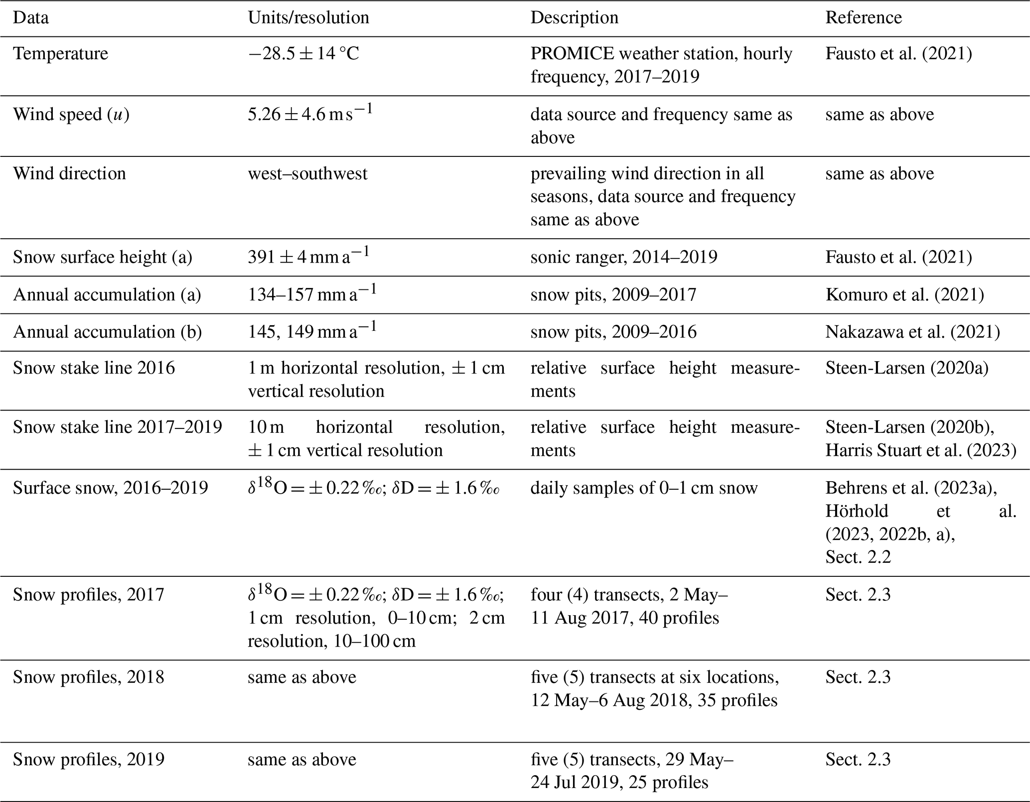
The data and products presented here are all derived from observations at the high-altitude EastGRIP ice core site located in northeast Greenland. In Sect. 2.1 we present the meteorological context of our study. In Sects. 2.2 and 2.3 we present the surface snow isotope and snow profile isotope data sets, respectively. In Sect. 2.3, we explain the siting, extraction, handling, and processing of the snow profiles. In Sect. 2.4, we discuss the age–depth model applied to the snow profile isotope data set. In Sect. 2.5 we discuss nuances and caveats relevant to the interpretation of the data presented here. Table 2 contains an overview of the data used in this study.

2.1 Meteorology: data and context

The EastGRIP site is located on a fast moving ice stream at 75°37^′47^′′ N, 35°59^′22^′′ W at an altitude of 2708 m (55 m a⁻¹; Westhoff et al., 2022). There is a PROMICE weather station located approximately 300 m south of our study site (Fausto et al., 2021). The mean annual temperature is −28.5 °C. The site experiences persistently high (5 m s⁻¹ ) and directionally constant winds because its location on the ice sheet results in downslope (westerly) katabatic winds and westerly synoptic flow over the ice sheet (Putnins, 1970; Dietrich et al., 2023).

Accumulation rates for EastGRIP just prior to the observation period derived from isotope profiles are approximately 134–157 mm a⁻¹ (Nakazawa et al., 2021; Komuro et al., 2021). Monthly surface height changes are continuous and greater in summer and autumn (68 %) than winter and spring (32 %), with approximately 50 % of the surface height changes coming from 20 % of the monthly accumulation for the period of 2014–2019.

2.2 Surface snow isotopes

The top 0–1 cm snow was collected along a 1000 m path parallel to the wind in the 2016 field season and a 100 m path for the 2017–2019 field seasons (Behrens et al., 2023a; Hörhold et al., 2023, 2022b, a). During the 2016 and 2017 field seasons, samples from each site were collected and bagged individually, the measured δ¹⁸O was then averaged. During the 2017 field season, snow of equal amounts was also collected daily at the same locations and then mixed into one sample bag, termed “consolidated” samples. It was found from this work that the mean isotopic values of the individually bagged samples were the same as the less laboriously obtained “consolidated” samples. Mean daily surface snow isotopic contents for the summers of 2018 and 2019 were therefore determined from “consolidated” samples. Surface snow was sampled to other depths during these field seasons, and we only use the 0–1 cm samples in this study.

Once collected, either individually or as a consolidated sample, the snow was sealed in an air-tight Whirl-Pak bag and kept frozen until measurement at the Alfred Wegener Institute in Bremerhaven, Germany, or the Institute of Earth Sciences in Reykjavík, Iceland. Isotopic measurement procedures for surface snow are the same as for the snow profiles and explained in Sect. 2.3.

2.3 Near-surface snow profile isotopes: siting, extraction, handling, and measurement

The central data presented here are isotope measurements from a time-resolved array of snow profiles from 0–1 m (Behrens et al., 2023b). The sampling strategy is diagrammed in Fig. 1. The snow profiles were taken along transects progressing in the windward direction. Each sampling event consisted of five snow profiles taken from five unique transect lines within a few hours of each other. The transect lines were at least 50 m from each other. A total of six transect lines were used but only five during any one sampling event.

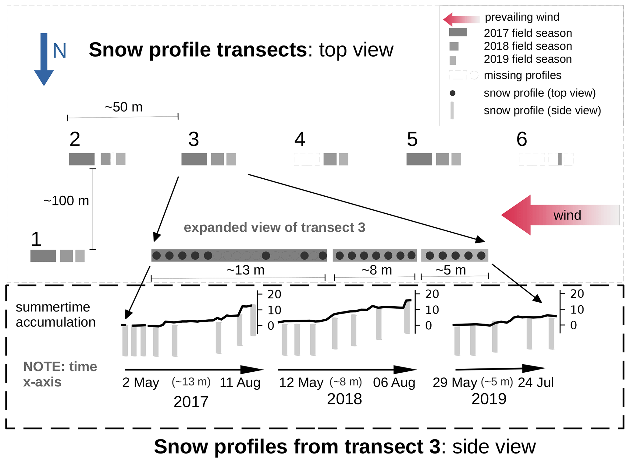
Figure 1 The top panel shows an overview of the relative spacing and timing of the transects along which the near-surface snow profiles were taken for this study. Each transect has the same snow profile pattern as Transect 3. The diagram is not to scale, but distances are noted. North is downward in this diagram. The prevailing wind direction is from the west–southwest. The number and relative timing of snow profiles are accurately indicated. The bottom panel shows an illustration of the summertime snow stake heights along with snow profile timing. The study site is the EastGRIP ice core site in northeast Greenland.

The frequency of snow profile sampling events ranged between 3 and 21 d, the most common frequency being 14 d. Snow profiles along one transect were spaced apart by approximately 1 m. The close spacing permits us to consider that most snow profiles along the same transect represent the same snow (See Sect. 2.5.1). A single snow profile was taken by gently pushing a 10 cm diameter carbon fiber tube (i.e., liner) with a 1 mm thick wall vertically into the snow. Minimal compression of the snow column occurs during this process (maximum 2 cm, average 1 cm; Schaller et al., 2016). A small pit was cleared on the downwind side of each liner so that they could be carefully extracted with all snow stratigraphically intact. The resulting snow pit was then back-filled within 2 h of beginning the process, mitigating exposure of deeper layers to the atmosphere above.

After extraction, each profile was quickly transported to a cold tent for cutting and storage. The profiles were cut at 1.1 cm resolution for the top 0–10 cm and 2.1 cm resolution for remainder of the profiles. Most profiles were not exactly 100 cm in length due to compression and a small amount of bottom loss during extraction. The snow was cut in an open-faced tray using a 1 mm thick blade. Each sample was sealed in an air-tight Whirl-Pak bag and kept frozen until measurement at either the Alfred Wegener Institute in Bremerhaven, Germany, or the Institute of Earth Sciences in Reykjavík, Iceland.

Measurements of δ¹⁸O and δD concentrations were made using a Picarro cavity ring-down spectrometer (models L2120-i, L2130-i, L2140-i) and reported in per mille (‰) notation as shown in Eq. (1) on the VSMOW–SLAP (Vienna Standard Mean Ocean Water and Standard Light Antarctic Precipitation) scale. Memory and drift corrections were applied using the procedure in Van Geldern and Barth (2012). We calculated the combined standard uncertainty (Magnusson et al., 2017) including the long-term uncertainty and bias of our laboratory by measuring a quality check standard in each measurement run and including the uncertainty of the certified standards. The combined 2σ uncertainty in δ¹⁸O is 0.22 ‰ and for δD is 1.6 ‰ for all isotopic measurements. We focus on δ¹⁸O and d for the remainder of this paper, as δ¹⁸O and δD are equivalent for our purposes. Propagation of errors makes the 2σ uncertainty in d equal to 2 ‰.

The snow cores we use are 1 m in length to capture at least two annual cycles at EastGRIP. Modeling also indicates this maximum depth will be well beyond the direct isotopic influence of the atmosphere (Town et al., 2008b). The spacing between transects (approximately 50 m) is well beyond established isotopic spatial autocorrelation lengths in polar snow (Münch et al., 2016), providing several independent realizations of the near-surface snow during each sampling event.

2.4 Intercomparison of chronological layers

2.4.1 Depth adjustment

Photogrammetric experiments at EastGRIP show that chronological layers of snow are continuous but inhomogeneous in thickness and spatial distribution (Zuhr et al., 2021b). This is in agreement with prior efforts documenting wind-driven erosion and deposition in snow (e.g., Fisher et al., 1985; Colbeck, 1989; Filhol and Sturm, 2015). Large precipitation events will have uneven representation in the snow, and in extreme cases (high winds with low accumulation) entire annual layers could be scoured at polar sites with low accumulation (e.g., Epstein et al., 1965; Casado et al., 2018). Zuhr et al. (2023) confirm the layers are continuous at EastGRIP, with only one exception in their spatial study. Zuhr et al. (2023) also documented that uneven surfaces and concomitant heterogeneous distribution of precipitation result in spatially heterogeneous isotopic concentrations of snow along perfectly horizontal transects. A horizontal average of δ¹⁸O or d then represents a mixture of events across time (Münch et al., 2017), particularly near the surface. Zuhr et al. (2023) estimates that the 2σ spread around horizontally average δ¹⁸O at EastGRIP is 2.9 ‰ due to the impact of this stratigraphic noise. Note that this number represents the distribution of the measurements, not the confidence in snow profile mean values.

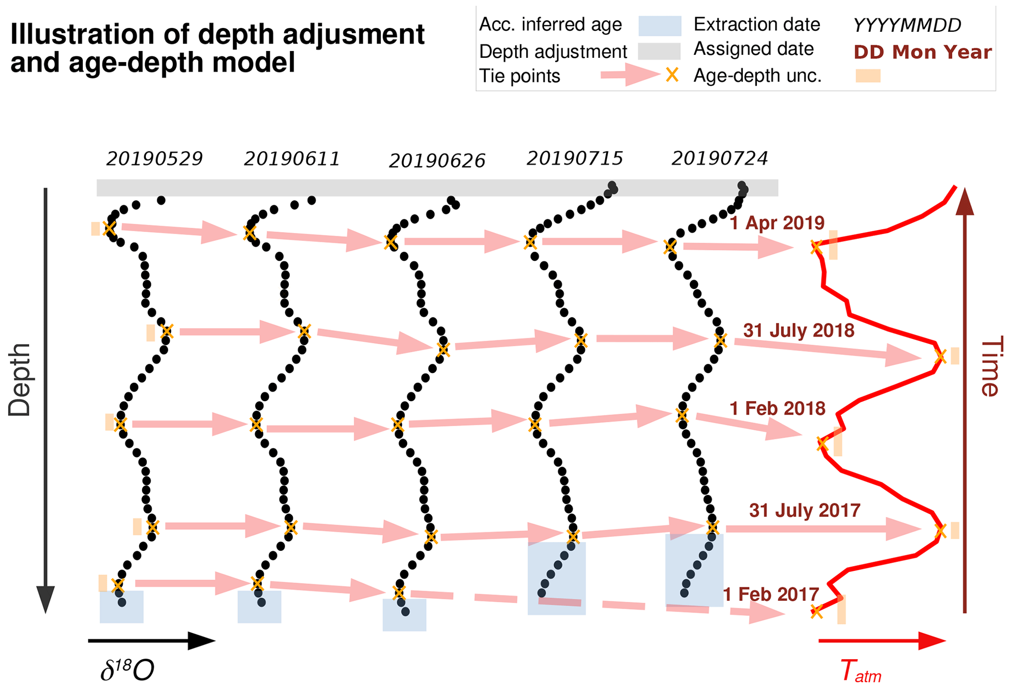
Figure 2 An illustration of the depth adjustment (gray range) and age–depth model applied to δ¹⁸O data from Transect 2 during the 2019 field season. The yellow crosses represent automatically found peaks in δ¹⁸O (black dots) and monthly mean 2 m temperature (red line). Each yellow star is assigned a date, and the intervening dates are linearly interpolated to a depth value. The lowest few δ¹⁸O data points are assigned by an iterative process based on the rate of change in surface height from that time period and then manually checked. Uncertainty in the snow profile peak identification and air temperature date assignment are illustrated in orange.

For this study, tracking chronological layers is critical to separate wind-driven spatial heterogeneity in δ¹⁸O and d from other processes at work in the near-surface snow. To better align chronological layers, we apply a local depth adjustment to individual snow profiles from 2018 and 2019 based on snow stake measurements of surface height changes at each sample site, illustrated in Fig. 2. For the 2017 snow profiles, we apply one depth adjustment to all profiles collected on the same day. We use the mean change in height from the 90 m snow stake transect to adjust snow surface height relative to the first profiles of the season collected on 2 May 2017 (Steen-Larsen et al., 2022). Compaction was not considered in the depth adjustment between snow profiles.

2.4.2 Age–depth model

The depth correction mitigates much of the stratigraphic noise induced by simple horizontal averaging but not all. We developed an age–depth model for each individual snow profile to further minimize stratigraphic noise in chronological layer intercomparisons within one season, also allowing better intercomparison of “same-era” snow (i.e., snow from the same time period) between profiles extracted during different field seasons.

An illustration of the age–depth model process is shown in Fig. 2 following similar seasonal and interannual studies (e.g., Shuman et al., 1995; Bolzan and Pohjola, 2000; Kopec et al., 2022). The end date for every profile is the extraction date, which is known precisely. From this date we worked downwards in the snow and backwards in time. Local maximum and minimum δ¹⁸O values were found automatically. Dates assigned to the δ¹⁸O values are from the maxima and minima in monthly mean temperature as measured at the nearby PROMICE weather station. We find at least two dates per annual layer: a summer maximum and a winter minimum.

The age–depth model depends on the continuity of layers between cores and serves to align layers to each other, as well as to the assigned dates. Although the age–depth scale is very accurate, much of our analysis depends primarily on the alignment of layers rather than the absolute date. The bottom of each snow profile was assigned dates based on contemporaneous surface height information from the sonic rangers.

The age–depth model uncertainty comes from two sources: (1) snow profile peak and trough identification and (2) maximum and minimum date attribution. The snow profile peak identification is more accurate near the top of the profiles because of sampling resolution. Maximum and minimum air temperature date attribution is more accurate in summer than winter. We conservatively assess the 2σ uncertainty as a minimum of ± 9 d for the top of each profile, ± 25 d around each summer peak below 10 cm, and ± 33 d around each winter trough below 10 cm.

A detailed discussion of the age–depth model and error analysis can be found in Sect. 2.5.3.

2.5 Snow isotope data set caveats and nuances

2.5.1 Decorrelation distances and snow profile comparisons

Our sampling and data processing strategy is designed to separate spatial and temporal variability in the isotopic content of the near-surface snow. The sampling strategy is inherently destructive, which results in trade-offs between accurate sampling and monitoring temporal variability. We attempt to balance these trade-offs by sampling at approximately 1 m spacing along each transect. The 1 m spacing keeps each profile well within established spatial decorrelation distances for spatially successive water isotope samples for a polar site with a similar altitude and accumulation rate (1.5 m; Münch et al., 2016). Sampling closer than 1 m along a transect risks disturbing the subsequent adjacent profile. The decorrelation distances derived in Münch et al. (2016) were done without application of spatial depth adjustment or an age–depth model to align chronological layers. Their decorrelation distances then represent an overestimate for our data set after the application of depth adjustments and an extreme overestimate after application of our age–depth model. Zuhr et al. (2023) show that isotopic continuity of layers is the rule rather than the exception at EastGRIP.

We collected samples as close together as possible so that snow profiles taken along one transect will be considered representative of the same snow, taking into account the small amount of stratigraphic noise observed on these spatial scales (e.g., Zuhr et al., 2023). During 2017 many (18) profiles were taken along each transect, although not all are used here (only 8). The reason for their removal is discussed in Sect. A1. The higher number of snow profiles represents a larger distance traveled over the history of the transect in 2017. It is very likely that the snow extracted from a transect at the beginning of the 2017 season does not represent the same location as the snow from the end of the 2017 season along the one transect. We consider this later when examining intraseasonal evolution of the near-surface snow.

The transect lines are separated by 50 m or more to provide “independent” representations of the near-surface snow. There will be no autocorrelation due to local dune and sastrugi features in same-day snow profile averages.

2.5.2 Mitigated biases due to sampling

We promptly back-filled each extraction site to mitigate the influence of near-surface meteorology on the next upwind profile. High temperature gradients take days to weeks to propagate through the snow at these distances (Town et al., 2008a). The potential influence of forced ventilation tapers off dramatically after about 50 cm depth in near-surface snow (Town et al., 2008b). So, our sampling procedure sufficiently prevents unintended post-depositional change due to extra exposure to the near-surface atmosphere. Other details related to missing data and uncertainties are shared in Appendix A3.

2.5.3 Age–depth models

Similar age–depth models have been developed using temperature-to-isotope data sets from the Greenland ice sheet. Higher-accumulation-rate sites like Summit, Greenland, allow more tie points in 1 year (e.g., Shuman et al., 1995; Bolzan and Pohjola, 2000). However, much lower resolution is also common. Kopec et al. (2022) assign 1 January to all winter δ¹⁸O minima. While this is problematic for absolute dating accuracy because of the quasi-coreless winter over Greenland, it does not change their conclusions. One tie point per year works in their study because Kopec et al. (2022) are concerned with relationships between variables measured in the snow, and Summit has a fairly constant accumulation rate, albeit having a seasonal compaction rate (Dibb and Fahnestock, 2004; Howat, 2022).

In our case, EastGRIP has approximately half the accumulation rate of Summit, Greenland; the accumulation rate varies with season (higher in summer and autumn, lower in winter and spring); and the compaction rate very likely has the same seasonality as Summit. We find at least two tie points each year, which is more than sufficient to resolve the seasonal accumulation and compaction at EastGRIP. The seasonal scaling applied to the δ¹⁸O and δD time series are the same, so the position of the d time series relative to δ¹⁸O remains the same. This will be important when evaluating the seasonality of d as the snow ages.

3 Results

We share results for surface and near-surface snow samples focusing on evolution during summer-only time periods (Sect. 3.1) separately from the interannual evolution of the snow profiles (Sect. 3.2). Their combined meaning is explored in Sect. 4.

Statistically, we are mainly concerned with how mean values compare even as distributions of these isotopic values and their derivatives may overlap. As such, most of our error values and uncertainty ranges are represented as 2 times the standard error around the means (2${\mathit{\sigma }}_{\stackrel{\mathrm{‾}}{x}}$, p<0.05). Where the overlap of distributions are important, we report 2 times the standard deviation around the mean (i.e., 2σ).

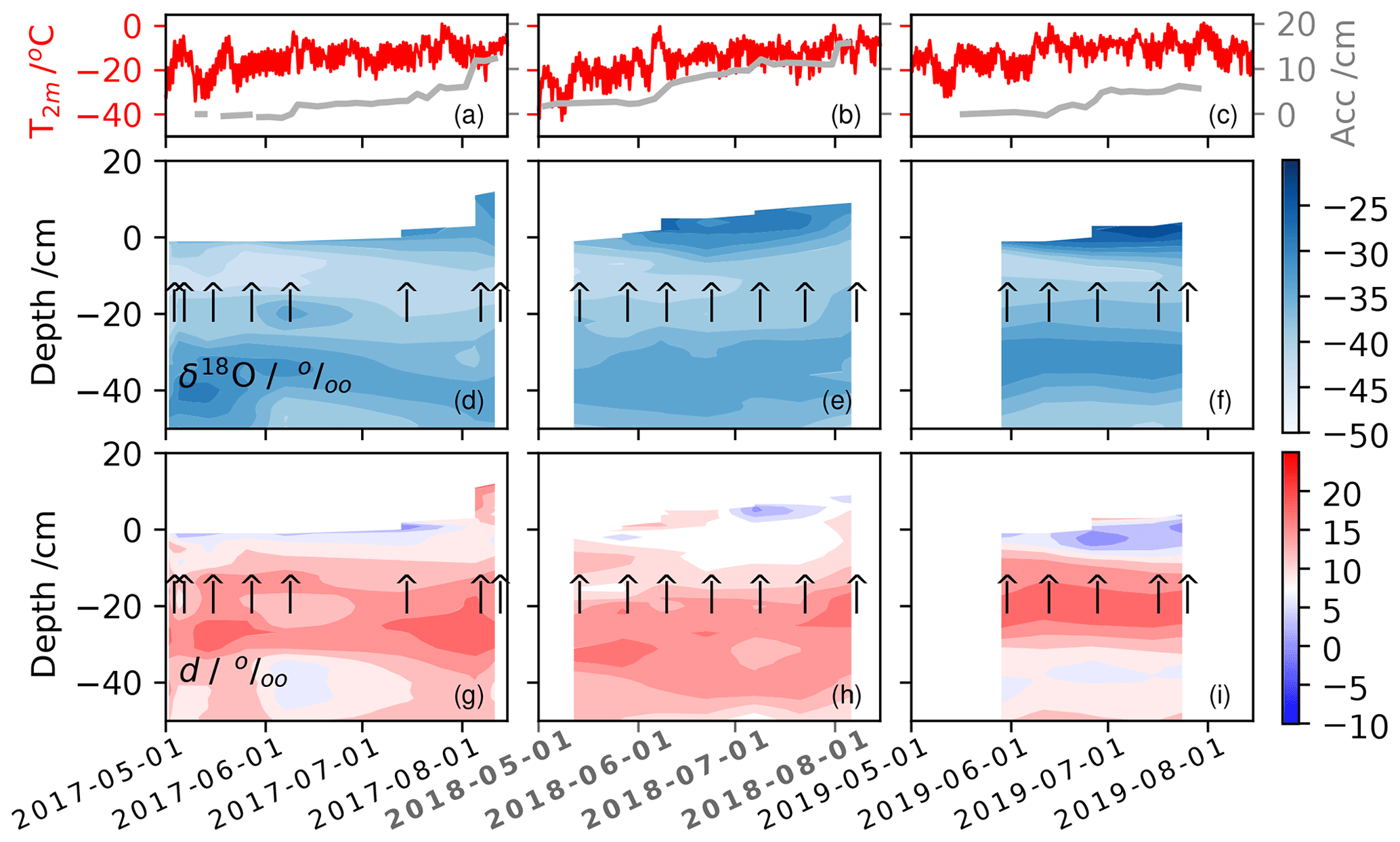
Figure 3 Mean δ¹⁸O and d snow profiles plotted as depth (vertical axis) and date of extraction (horizontal axis) for the three summer field seasons 2017, 2018, and 2019. Panels (a)–(c) show the 2 m air temperature from the local PROMICE weather station and accumulation from the bamboo stake line. Panels (d)–(f) show the δ¹⁸O content of the near-surface snow determined from mean δ¹⁸O snow profiles. Each arrow represents a mean snow profile spaced approximately 50 m from another (four snow profiles in 2017, five snow profiles in 2018 and 2019). Panels (g)–(i) are similar contour plots but for d. Note the vertical axis only extends to 50 cm depth.

3.1 Summer season δ¹⁸O and d

Figure 3 provides a look at the isotopic evolution of the near-surface snow during the summer field seasons. The extraction dates (upward arrows), 2 m air temperature, and mean surface height changes from the bamboo stake line are provided for context. The mean surface height changes do not match up exactly with the height changes in the contour plots below because they were in different locations. Each upward arrow represents the mean of four or five snow profiles taken on the same day from different transects. Aggregating the snow profiles in this manner likely mitigates much spatial variability. We show the first annual cycle (0–50 cm) because there is no detectable subseasonal change below approximately 10–15 cm on these timescales, consistent with modeling by Waddington et al. (2002) and Town et al. (2008b).

The top 10–15 cm in Fig. 3 shows an enrichment pattern in δ¹⁸O during low-to-no accumulation periods, with a coincident decrease in d. In the lower parts of the profiles, the strength of the δ¹⁸O annual signal smoothens likely due to IGD diffusion and temperature-gradient-driven diffusion. Figure 3 does not illustrate a clear temporal change in d profile on this timescale below about 20 cm. Although the patterns illustrated in the very top snow layers are strong, they are complicated by accumulation. These data show that new accumulation can bring in a range of δ¹⁸O values to the surface snow, but typically new accumulation has a high (≥ 10 ‰) d content.

Figures 4–6 illustrate in a different way how mean daily profiles (four to five profiles) change during similar low-to-no accumulation periods. We chose as similar time periods for this comparison as possible, attempting to match period length, the time of year, and low-to-no accumulation. Significant increases (p<0.05) are δ¹⁸O seen only in the summer 2019 down to 10–15 cm (Fig. 6). A similar pattern is shown for δ¹⁸O for 2017. Both periods show coincident decreases in d in the top snow layers, albeit insignificant in these data. Temporal changes in the 2018 snow profiles are not so easily encapsulated in the mean profile difference plot shown. In this case, not only is there is no significant change in δ¹⁸O and d over the chosen low-to-no accumulation period, but the Δδ¹⁸O is the opposite of the other two summers for this time period. Other periods during 2018 may show significant differences in their profiles, but we choose here to keep the time periods as similar as possible for this illustration.

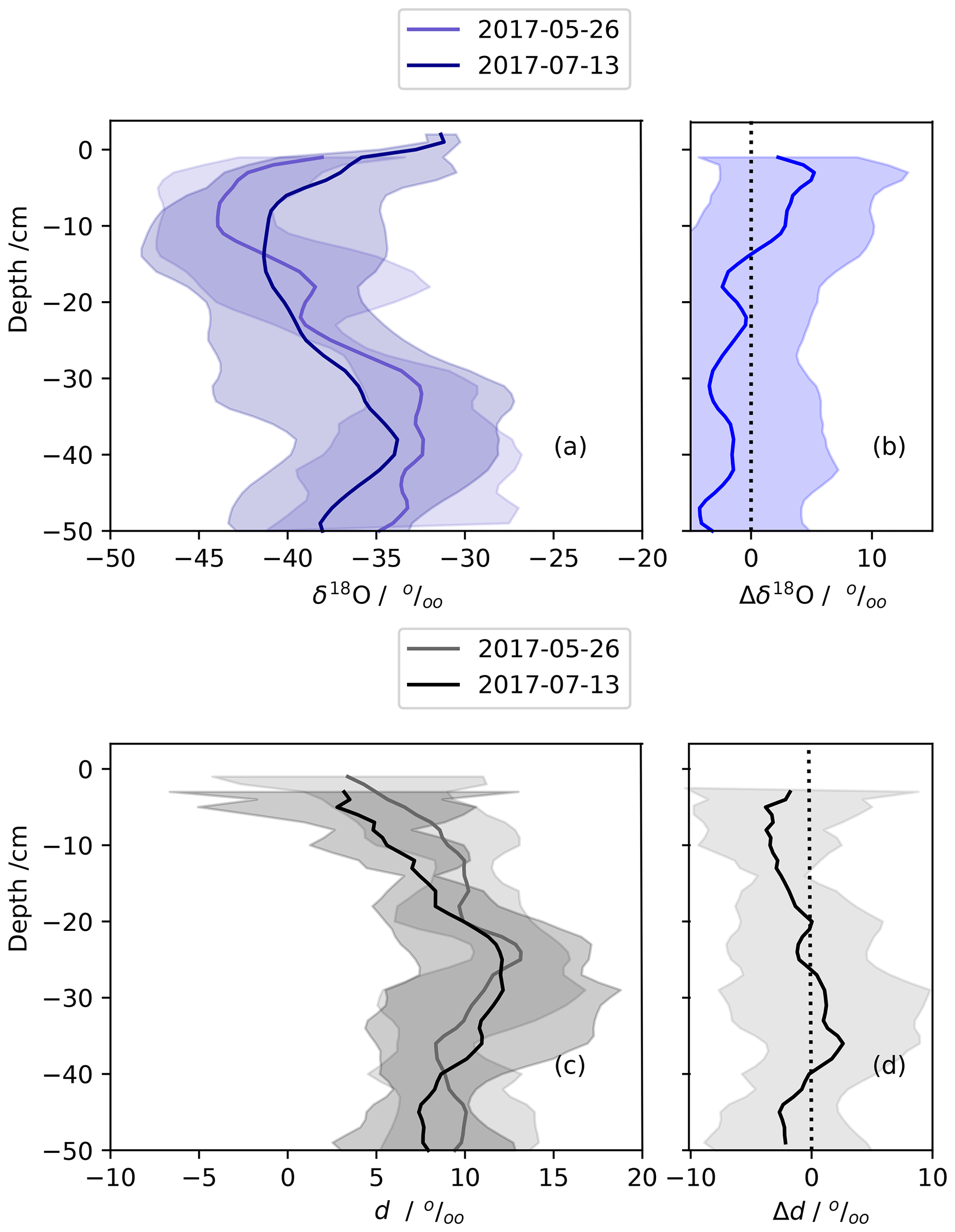
Figure 4 The mean isotopic change in the near surface from a low-accumulation period during summer (25 May and 13 July 2017). Panels (a) and (c) are the mean snow profiles of δ¹⁸O and d computed from four snow profiles each. Panels (b) and (d) show the isotopic change over this time period. Error bars are 2σ standard error.

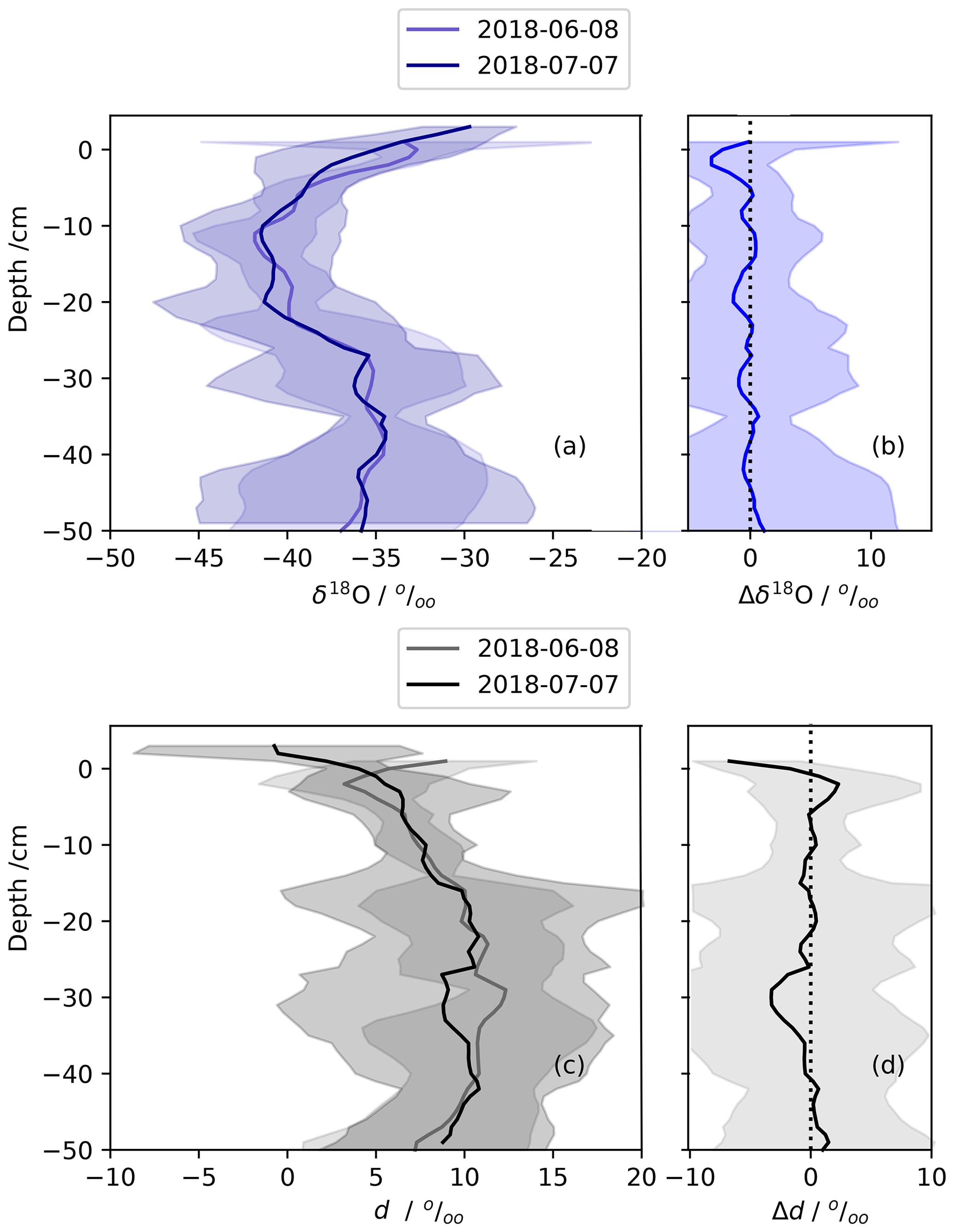
Figure 5 The mean isotopic change in the near surface from a low-accumulation period during summer (8 June and 7 July 2018), similar to Fig. 4. Panels (a) and (c) are the mean snow profiles of δ¹⁸O and d computed from five snow profiles each. Panels (b) and (d) show the isotopic change over this time period. Error bars are 2σ standard error.

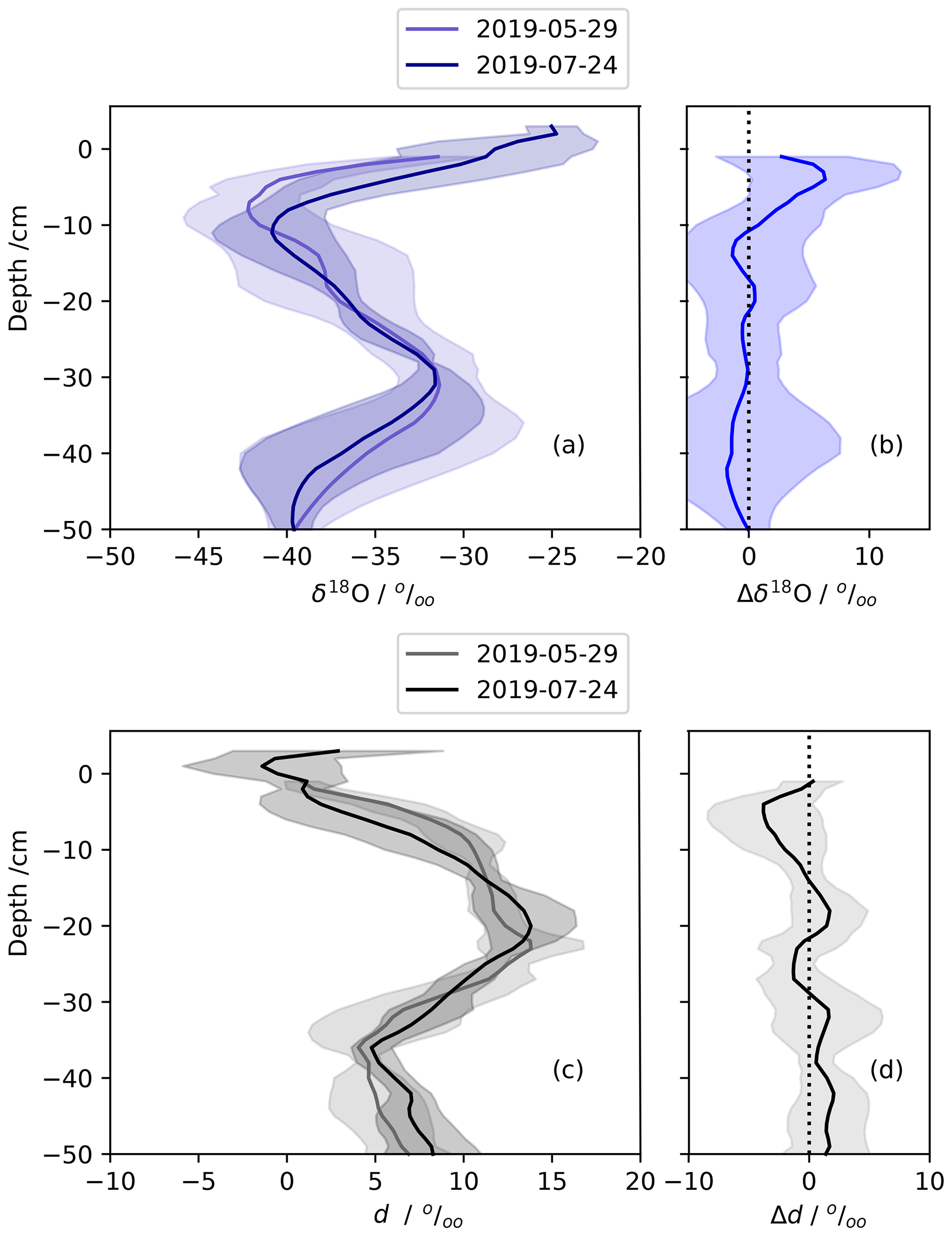
Figure 6 The mean isotopic change in the near surface from a low-accumulation period during summer (29 May and 24 July 2019), similar to Fig. 4. Panels (a) and (c) are the mean snow profiles of δ¹⁸O and d computed from five snow profiles each. Panels (b) and (d) show the isotopic change over this time period. Error bars are 2σ standard error.

On the other hand, when comparing surface snow samples to same-era snow from a snow profile from the same summer in 2018 and 2019, we see a 5 ‰ decrease in d; the same decrease in d is not apparent in the 2017. The d decreases are discussed in Sect. 4.1.1, illustrated in Fig. 8c, and shown in Table B5.

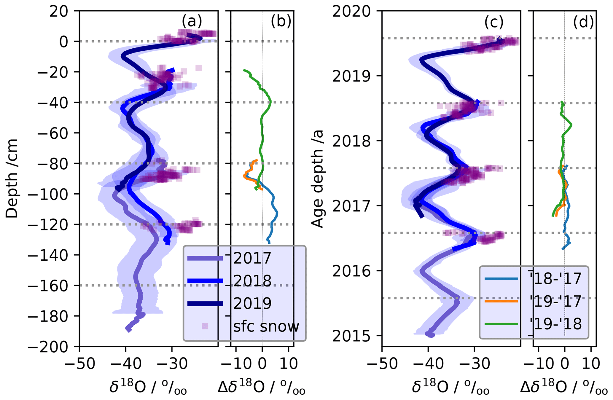
Figure 7 Mean δ¹⁸O values from snow profiles and surface snow. The surface snow data (purple squares) are daily means from the 2016–2019 summer seasons. The snow profiles are mean values grouped by year of extraction (e.g., 2017, 2018, and 2019). Panel (a) shows the mean surface snow and snow profile δ¹⁸O values as a function of relative depth. The surface is defined as 29 May 2019, the first day of snow profile sampling in 2019. Panel (b) shows the difference between each profile as a function of relative depth, representing the interannual change in δ¹⁸O. Panel (c) shows the mean surface snow and snow profile δ¹⁸O values as a function of age–depth. Panel (d) shows the difference between each profile as a function of age–depth, representing the interannual change in δ¹⁸O. Shading represents 2σ standard error (2${\mathit{\sigma }}_{\stackrel{\mathrm{‾}}{x}}$). The horizontal lines in panels (a) and (b) are set at 40 cm, the approximate annual snow accumulation rate at EastGRIP. The horizontal lines in panels (c) and (d) represent 31 July of each year.

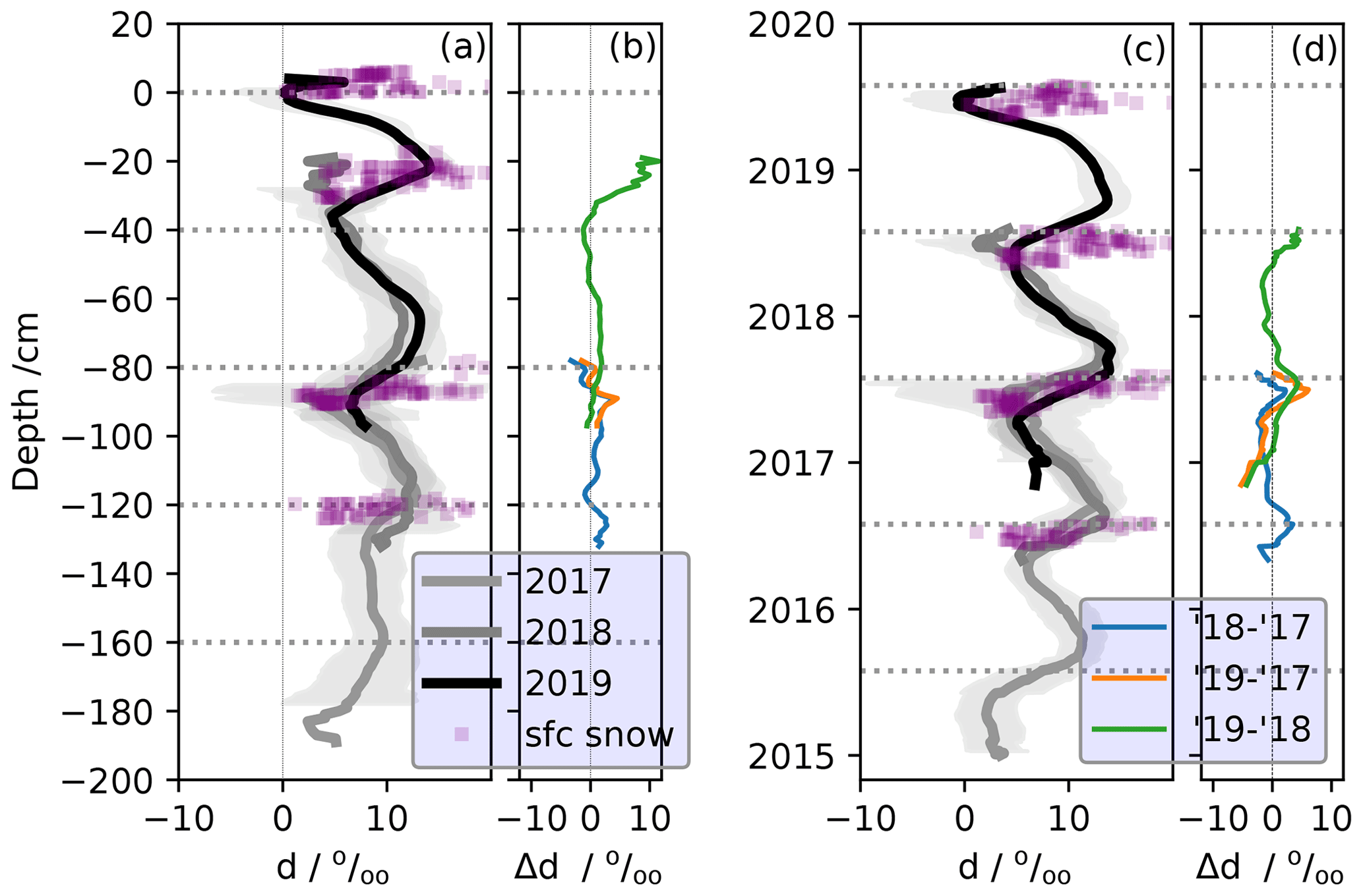
Figure 8 Mean d values from snow profiles and surface snow, as in Fig. 7 for δ¹⁸O. The surface snow data (purple squares) are daily means from the 2016–2019 summer seasons. The snow profiles are mean values grouped by year of extraction (e.g., 2017, 2018, and 2019) with 2${\mathit{\sigma }}_{\stackrel{\mathrm{‾}}{x}}$ as the shading. Panel (a) shows the mean surface snow and snow profile d values as a function of relative depth. The surface is defined as 29 May 2019, the first day of snow profile sampling in 2019. Panel (b) shows the difference between each profile as a function of relative depth. Panel (c) shows the mean surface snow and snow profile d values as a function of age–depth. Panel (c) shows the difference between each profile as a function of age–depth. Panels (b) and (d) represent the change in d between the different field seasons. Shading represents 2σ standard error (2${\mathit{\sigma }}_{\stackrel{\mathrm{‾}}{x}}$). The horizontal lines in panels (a) and (b) are set at 40 cm, the approximate annual snow accumulation rate at EastGRIP. The horizontal lines in panels (c) and (d) represent 31 July of each year.

3.2 Interannual δ¹⁸O and d

Figures 7 and 8 show annually successive surface and near-surface snow isotopic content for δ¹⁸O and d, respectively. Figures 7a and 8a show the mean profiles as a function of relative depth with shading as 2 times the standard error (2${\mathit{\sigma }}_{\stackrel{\mathrm{‾}}{x}}$). The 0 m level was chosen as 29 May 2019, the day the first snow profile was extracted during 2019. Figures 7b and 8b show the difference between each profile as a function of relative depth. These difference profiles represent the isotopic change due to aging in the firn because the same-era layers have been aligned through the depth correction, although some spatial variability no doubt remains.

Figures 7c and d and 8c and d show the same isotopic data as in their respective panels (Figs. 7a, b and 8a, b) but are now plotted as a function of the age–depth model described in Sect. 2.4.2. The age of a given snow profile ranges from 2 to 3 years depending on the total accumulation rate for that time period and exact location. Taken as a whole, the dates represented by the snow profiles span 2014–2019. The age–depth model inherently better aligns chronological layers than the depth adjustments, further mitigating impacts of spatial inhomogeneity in stratigraphy and densification on the quantitative comparison of δ¹⁸O and d in snow layers. This can be seen in a decrease in 2${\mathit{\sigma }}_{\stackrel{\mathrm{‾}}{x}}$ values from panel a to panel c in Figs. 7 and 8, particularly for the 2017 snow profiles.

Figure 10 shows the difference between annually successive mean snow profiles. It is similar to panel d from Figs. 7c and d and 8 but with 2${\mathit{\sigma }}_{\stackrel{\mathrm{‾}}{x}}$ shading. Figure 10 can be interpreted as how δ¹⁸O and d evolve 1 or 2 years after being buried, now as a function of reference snow profile age.

Using the summer δ¹⁸O profile peaks as annual markers, we find a mean annual snow accumulation rate across all snow profiles of 45.6 ± 3.8 cm (13.5 ± 1.1 $\mathrm{cm}{\mathrm{a}}^{-\mathrm{1}}\mathrm{l}.\mathrm{w}.\mathrm{e}.$) for this time period (2014–2019) consistent with other isotopically derived accumulation rates for EastGRIP (Nakazawa et al., 2021; Komuro et al., 2021). Annual and seasonal statistics from Figs. 7 and 8 are shown in Tables B1–B4 in Appendix B.

3.2.1 Interannual evolution of δ¹⁸O

Mean annual δ¹⁸O values are fairly constant throughout this time period regardless of aging, approximately −36 ‰. However, there is significant variability in the peak summer δ¹⁸O in each profile, regardless of snow age. The 2019 summer has the greatest peak δ¹⁸O values. There is not concomitant variability in the minimum winter δ¹⁸O values in this record. Some differences between profiles seem significant when plotted against relative depth (Fig. 7b). However, when the age–depth model is applied, differences between profiles show no significant interannual change in δ¹⁸O (Figs. 7d and 10a).

During the season of extraction, the surface snow δ¹⁸O values (purple squares) and mean summer snow profile δ¹⁸O values match and have approximately the same variability for this period. After aging 1 year, the mean snow profile δ¹⁸O for July 2018 extracted in 2019 matches the mean surface snow δ¹⁸O. However, the surface snow δ¹⁸O from 2016 and 2017 is several per mille enriched over the snow that has aged 1 or 2 years (Fig. 7c, d).

3.2.2 Interannual evolution of deuterium excess (d)

The interannual variability and seasonal cycles of deuterium excess are shown on both depth and age–depth scales in Fig. 8. The snow profiles show an annual d cycle at EastGRIP of approximately 10 ‰–15 ‰ in magnitude, whereas the surface snow shows d values as high as 20 ‰ in summer. The minima occur during the spring and summer, while the maxima occur during autumn at the top of the profiles. This changes as the profiles age, with differences between d profiles extracted during different field seasons showing a distinct peak in the summer layers (Figs. 8d and 10b). These profile data demonstrate significant differences between summer d values from surface snow (purple squares) and the snow profiles during the season of extraction. The mean surface snow d is 10.3 ± 2.5 ‰ and 8.1 ± 2.4 ‰ during the summers of 2018 and 2019, respectively, whereas the mean snow profiles show d values of only 5.4 ± 0.5 ‰ and 3.7 ± 0.6 ‰, for the summers of 2018 and 2019, respectively. This represents an increase in d of the surface snow of approximately 5 ‰ in both summer season snow layers (Fig. 3h and i and Table B5). In 2017, d in the summer snow profile is less than surface snow, but the difference is insignificant.

After aging for 1 year, the same summer layer d has increased by as much as 5 ‰ because the autumn maximum peaks broaden into summer and spring layers. Although not exceeding 2${\mathit{\sigma }}_{\stackrel{\mathrm{‾}}{x}}$ significance, there is also a persistent decrease in winter d values shown in Fig. 8d as the snow ages interannually. The mean annual d values of the snow profiles do not change from year-to-year, regardless of aging (Table B3).

4 Discussion

There are significant changes in the isotopic content of near-surface snow after deposition at the EastGRIP site. We observe these changes occurring on two timescales: during the summer season and interannually. The largest changes we observe are in the summer snow layers on both timescales. Enrichment in δ¹⁸O and a decrease in d can happen during the summer season in the top 20–30 cm of snow during low-to-no accumulation periods. A subsequent increase in d in the summer snow layer occurs as the snow ages 1 or 2 years in the firn. Below we discuss potential mechanisms for these processes and their implications and make recommendations for future work.

4.1 Post-depositional isotopic processes at EastGRIP

The phenomenon of post-depositional isotopic modification is driven by latent heat fluxes to and from the snow surface and latent heat fluxes within the near-surface snow (i.e., snow metamorphism). As a primarily observational effort, we are able to make strong inferences about potential mechanisms through compositing and context, but we also use two models of relatively simple complexity to help constrain our inferences. The first model simulates IGD diffusion within the snow (Johnsen et al., 2000), a mechanism of snow metamorphism and a smoothing influence of isotopic signals in snow. The implementation of this concept is taken from the SNOWISO model (Wahl et al., 2022) and is unaltered for our use. The second model simulates the influence of atmospheric vapor deposition and snow sublimation on internal snow layers through a forced-ventilation model in snow (Town et al., 2008b). The handling of isotopes in Town et al. (2008b) has been improved from only representing equilibrium fractionation during deposition of δ¹⁸O to include (1) δD, (2) an improved equilibrium fractionation representation (Stern and Blisniuk, 2002), (3) fractionation on sublimation for both species (Lécuyer et al., 2017; Hughes et al., 2021; Wahl et al., 2022), and (4) kinetic fractionation (Jouzel and Merlivat, 1984). This model empirically combines atmosphere-to-surface latent heat flux with snow metamorphism by assuming that the atmosphere can communicate directly with subsurface snow layers. Almost all forced-ventilation simulations use kinetic fractionation, with two simulations done with equilibrium fractionation for reference (See Appendix D).

4.1.1 Mechanisms at work during summer

In Sect. 3.1 we show evidence of a dramatic decrease in d over the summer period of approximately 5 ‰ but no significant change in δ¹⁸O in two summer seasons (2018 and 2019) when comparing daily surface snow samples to same-era mean snow profiles. We see moderate evolution of δ¹⁸O (enrichment) and d (decrease) in the top 20 cm of the snow profiles as the snow ages through the summers of 2018 and 2019 (Fig. 3e and f) under low-to-no accumulation periods.

Standard interpretations of a 5 ‰ shift in d could be either a 5 K cooling of source-region sea surface temperatures or a 10 % increase in source-region relative humidity (Pfahl and Sodemann, 2014). While there is clear evidence that d of precipitation does carry source-region information (Dansgaard, 1964; Craig and Gordon, 1965; Merlivat and Jouzel, 1979; Jouzel and Merlivat, 1984; Pfahl and Sodemann, 2014) and air mass transport (e.g., Markle and Steig, 2022), the observations presented here challenge that interpretation.

Recent evidence demonstrates that a decrease in d, often associated with an increase in δ¹⁸O, is a likely signal of sublimation (Hughes et al., 2021; Wahl et al., 2022; Harris Stuart et al., 2023). We see mild Δd within the near-surface snow down to 10–15 cm throughout the summer as compared to the dramatic Δd when comparing mean d from surface snow and mean d from the same-era snow profile. From this, we infer that much of the Δd occurs at the snow surface before it is advected away from direct contact with the atmosphere by burial. This is consistent with observations and modeling of isotopic fractionation under summertime sublimation conditions at EastGRIP (Wahl et al., 2022). Our observations are further corroborated by a contemporaneous, high-resolution, DEM-based spatial isotope study of EastGRIP snow, completed in summer of 2019 (Zuhr et al., 2023). Using daily photogrammetry and spatially distributed short cores (30 cm), they also observed a decrease in d of up to 5 ‰ and no significant change in δ¹⁸O. The change in d was concentrated in the top 5–20 cm of snow.

Challenges to the interpretation of our observations are in two categories: (1) attribution of variability temporally vs. spatially and (2) seasonal intermittency. It is clear that some variability we represent as temporal in Fig. 3 can potentially be attributed to spatial heterogeneity. However, we believe this is minimal because the mean profiles are aggregated from individual profiles spaced approximately 50 m apart. So, they are immune to autocorrelation induced by wind-formed surface features, which are commonly 1–2 m in length but can have widths of up to 10 m (Filhol and Sturm, 2015). Furthermore, low-to-no accumulation periods generally exhibit increases in δ¹⁸O and decrease in d, an established isotopic “sublimation” signal (Wahl et al., 2022). Alternatively, low-to-no accumulation periods do not show other combinations of changes in δ¹⁸O and d.

The summertime signals are inconsistent interannually even when composited by low-to-no accumulation, emphasizing the point that post-depositional isotopic change in near-surface snow is likely induced by local meteorology. The influence of the atmosphere on surface and near-surface snow is of primary concern during low-to-no accumulation time periods, but mechanical mixing is also of concern. Wind-driven redistribution complicates any interpretation, itself likely a source of local climate signal. Toppling of surface hoar and facets by winds (Gow, 1965) can be a significant imprinting and redistribution mechanism at EastGRIP. Excursions of entire seasons are possible at low-accumulation sites (e.g., Epstein et al., 1965). Zuhr et al. (2023) very likely identify a missing winter layer at one of their locations, although they do not resolve an entire annual cycle in any profile. Unraveling these processes for EastGRIP, or any site, likely requires a process-based approach to constrain the contribution of relevant phenomena.

4.1.2 Modeling of summertime post-depositional processes

We further explore the summertime results through idealized simulations to constrain inferences from the observations. The first simulation employs Johnsen et al. (2000) for the steepest mean isotopic gradients from our snow profiles (i.e., the top of the profiles) for an extreme idealized annual cycle. There is an attenuation in peak δ¹⁸O of up to 2 ‰ due to IGD diffusion (not shown). The simulated changes in peak δ¹⁸O for only summer is less than changes in δ¹⁸O over 47 d in 2017 and 2019 (Figs. 4a, b and 6a, b). It is also beyond our ability to definitely discern this with these observations. Dramatic shifts in d appear in the diffused profiles, with paired positive and negative residuals due to the flattening and shifting on the d annual cycle (See Fig. 11). This is similar to the pattern shown in Fig. 10 with the notable absence of the negative residuals, indicating that additional processes are likely at work in the near-surface snow.

The next simulations investigate the potential influence of the atmosphere on the near-surface snow through forced ventilation using a modified version of the forced-ventilation model from Town et al. (2008b). In these idealized scenarios, we simulate interstitial sublimation and deposition conditions in polar snow induced by the atmosphere during idealized EastGRIP summer season conditions. All assumptions about the model snow properties, fractionation, and scenario conditions are summarized in Table D1; salient features are discussed here. The model snow begins with an isotopic profile of δ¹⁸O_snw = −30 ‰ and d_snw = 10 ‰ and is allowed to change as water vapor deposits or sublimates. The atmospheric water vapor is set to δ¹⁸O_atm = −40 ‰ and d = 10 ‰. The atmospheric value is constant throughout the simulations, assuming the boundary layer drives isotopic content as it does in relatively windy places like NEEM (Steen-Larsen et al., 2014). We assume ice saturation at all temperatures. All fractionation is considered to be kinetic based on Jouzel and Merlivat (1984). We set the snow surface structure with undulations of 1 m peak-to-peak length and 0.10 m half-height; the feature sizes were chosen to represent summer snow conditions at EastGRIP (Zuhr et al., 2023) and be compatible with the model parameterizations (Colbeck, 1997; Waddington et al., 2002; Town et al., 2008b).

The deposition scenario, FV_dep, is driven by a prescribed temperature difference between the surface atmosphere (T_atm = −10 °C, a typical mean July air temperature for EastGRIP) and near-surface snow (T_snw = −15 °C). This can be considered early EastGRIP summertime conditions when the air temperatures are on average higher than snow temperatures. The assumption of ice saturation dictates that warmer saturated air deposits excess vapor in pore spaces as it is forced into the snow, thereby modifying the δ¹⁸O and d signals. The sublimation scenario, FV_sub, has the reverse conditions. These can be considered late summertime EastGRIP conditions when air temperatures are on average colder than snow temperatures. Under these conditions, colder, saturated surface air warms as it enters the snow, sublimating interstitial mass as the pore spaces achieve saturation.

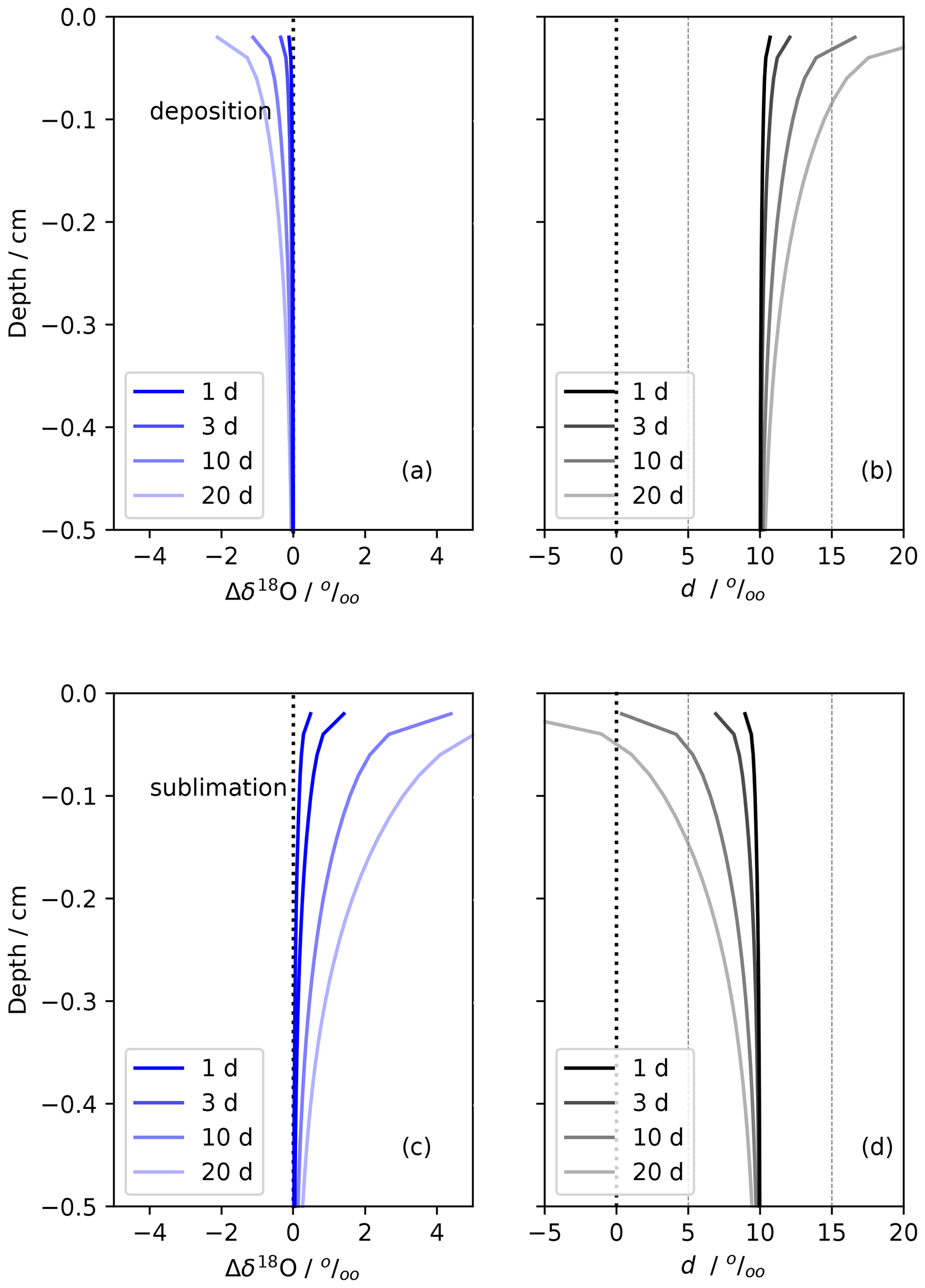
Figure 9 Idealized simulations of forced ventilation on isotropic snow under typical EastGRIP summertime conditions. Panels (a) and (b) show deposition for δ¹⁸O and d, respectively. The deposition conditions are FV_dep, T_snw = −15 °C, T_atm = −10 °C, and u = 5 m s⁻¹. Panels (c) and (d) show sublimation for δ¹⁸O and d, respectively. The sublimation conditions are FV_sub, T_snw = −10 °C, T_atm = −15 °C, and u = 5 m s⁻¹. The snow structure and isotopic content of snow and vapor are detailed in Table D1. This simulation assumes kinetic fractionation. Similar simulations are shown in Sect. D2: kinetic fractionation simulations with u = 10 and 20 m s⁻¹ and equilibrium simulations with u = 5 m s⁻¹.

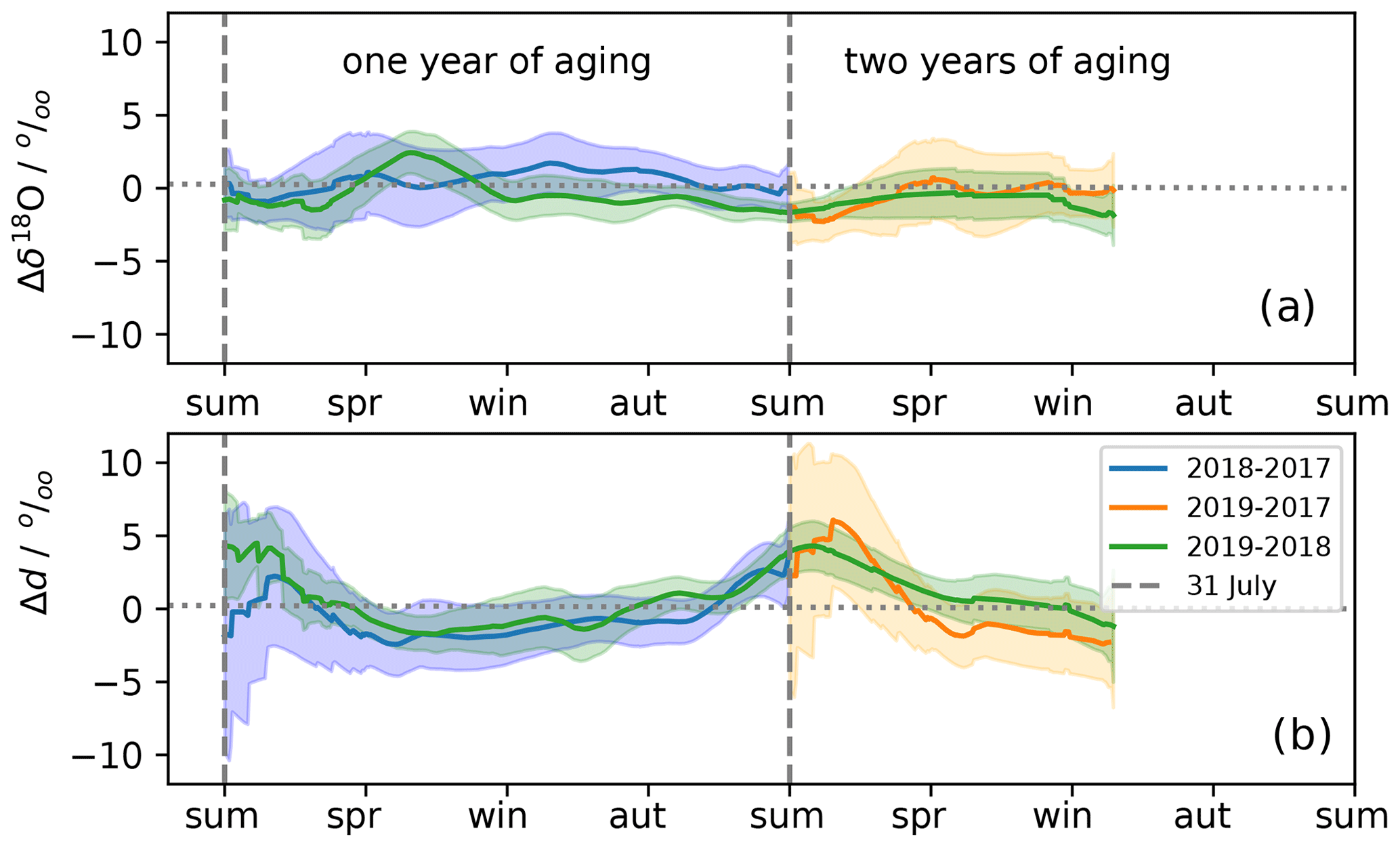
Figure 10 The change in δ¹⁸O (a) and d (b) after 1 to 2 years of aging in the near-surface snow. The change is determined as the difference between profiles shown in Figs. 7c and 8c and plotted as a function of the age of the reference profile in the difference. Seasons are marked on the horizontal axis, with snow depth increasing and time decreasing to the right.

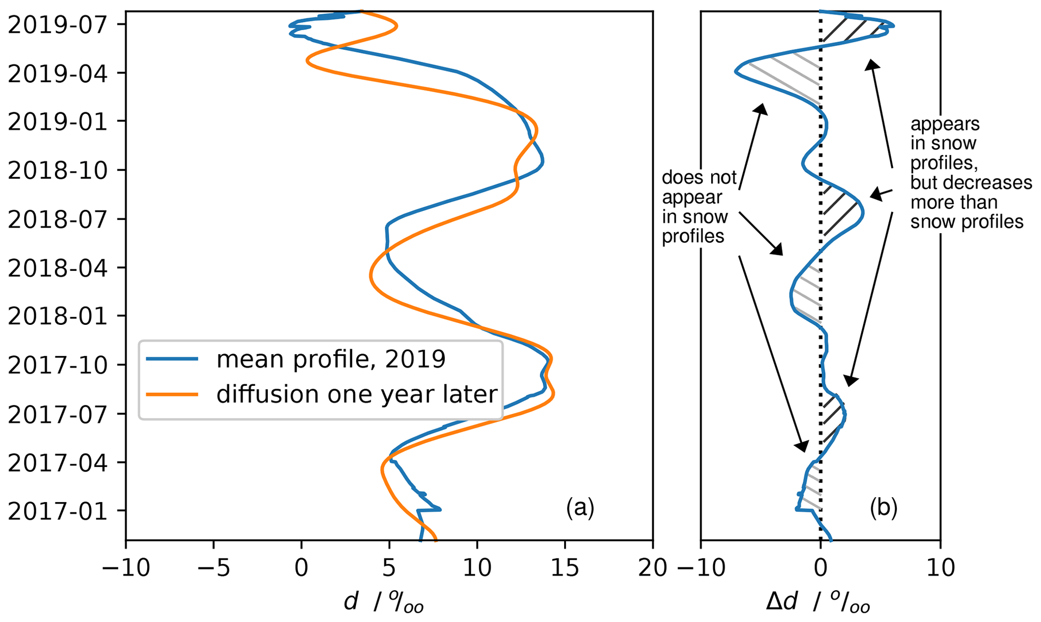
Figure 11 Annual isotope-gradient-driven diffusion scenario. Panel (a) shows a simulation of the impact of isotopic-gradient-driven diffusion on the mean d snow profile from 2019 (blue curve) after 1 year of aging (orange curve). Panel (b) shows the change in d (Δd) after 1 year of aging. The simulation is described in detail in Sect. D1.

Figure 9 shows how the model-predicted vapor exchange with the atmosphere will change with surface winds of 5 m s⁻¹, the mean annual and mean summertime wind speed for EastGRIP. The model predicts the impact is largest at the surface and tapers to insignificant levels by 20–30 cm depth. The FV_sub scenario predicts an increase in δ¹⁸O and a decrease in d, while the FV_dep predicts the reverse. It is worth noting that summer is dominated by sublimation, so the FV_sub modeling results for a 3–10 d period, a typical low-to-no accumulation period, indicate a decrease in d of approximately 5 ‰. This is consistent with our observations and the work of others at EastGRIP (Dietrich et al., 2023; Wahl et al., 2022). The FV_dep results show less dramatic increases in d but are also consistent with the magnitude of the negative residuals in Fig. 11b but missing from Fig. 10. Of course, the absolute magnitude of the modeled changes depends on the amount of time spent under these conditions.

These scenarios are idealized and only intended to help constrain interpretation of our results. The magnitude, direction, and depth of the modeled changes are consistent with changes observed in snow profile during low-to-no accumulation periods at EastGRIP during summer (Fig. 3). Our results indicate the atmosphere likely has a significant influence on the near-surface snow during relatively warm summer months. The sign and magnitude of a parameter like Δδ¹⁸O:Δd may help characterize climates as sublimation or deposition climates, aiding interpretation of paleorecords when post-depositional isotopic change is suspected.

From a meteorological point of view, an important nuance is the combined choice of wind speed and length of simulation. We provide several combinations. A typical sustained wind speed at EastGRIP is 5 m s⁻¹ due to its location, slope, and elevation in northeast Greenland. Higher wind speeds occur for much shorter durations, which we also simulate (Figs. D1 and D2). The shorter but more intense events have similar impacts isotopically on the near-surface snow. However, higher wind speeds do have the theoretical ability to reach deeper into the snow, as occurs in our model. We have also run the scenarios shown in Fig. 9 under equilibrium fractionation conditions for reference (Fig. D3).

The assumptions of temperature in these scenarios are meant to represent the steady warming and cooling of the summertime snow. The same scenarios can also represent typical maximum and minimum diurnal temperatures. Larger variations occur on this timescale, but the temperature gradients penetrate less deeply into the snow on diurnal timescales. The impact of these processes drops dramatically with temperature during the other seasons.

Other vulnerabilities in this modeling approach exist besides the simple assumptions about summer climate or the controlled physical processes simulated. Although the snow structure is based on Zuhr et al. (2023), it is also idealized. Zuhr et al. (2023) and others (e.g., Gow, 1965) show that surface relief on high-altitude ice sheets decreases throughout the summer. More complicated representations are possible but likely with marginal returns. We simulate the mean impact of force ventilation, but the physical phenomenon of snow ventilation varies spatially under the heterogeneous surface. Dunes and sastrugi migrate under blowing snow conditions (Filhol and Sturm, 2015), although this is not a pronounced effect in summer when the snow surface tends to solidify and flatten. Thus, the processes modeled here may represent an additional source of isotopic heterogeneity in addition to the heterogeneous filling observed at EastGRIP (Zuhr et al., 2021b, 2023).

The model assumes direct exchange of air between the atmosphere and each snow depth. This does not happen; very likely vapor exchange is layer to layer through the snow. Kinetic fractionation does occur in the snow, but it is more likely driven by vapor-pressure gradients induced by interstitial temperature gradients than direct vapor exchange with the atmosphere. The time constants that underpin the model of surface-to-subsurface vapor exchange (Waddington et al., 2002) accommodate this weakness of the model, effectively parameterizing a net vapor exchange with the atmosphere. Nevertheless, interstitial transport is an area of improvement for the model.

Laboratory experiments of isotopic evolution of snow under high-flow-rate forced ventilation (2 L min⁻¹) show isotopic changes similar in magnitude to those observed and modeled here. However, the changes only extend to layers of thickness up to 3 cm (Hughes et al., 2021). Further study should be done to unify these approaches to understand the potential impact of the near-surface atmosphere on near-surface snow.

4.1.3 Mechanisms at work interannually

In our interannual analysis, inferences about the influence of the summertime atmosphere on the near-surface snow are strongest because the snow profiles were extracted during the summer season. However, inferences about the influence of other seasons are possible as the snow profiles typically extend approximately 2.5 years.

Interannual Δδ¹⁸O. There are no significant changes in δ¹⁸O (Δδ¹⁸O) between the mean snow profiles extracted during different summers (Figs. 7c, d and 10a). Figure 10a shows similar information to Fig. 7d, but here the Δδ¹⁸O is a function of the reference year age and depth. In other words, it shows Δδ¹⁸O after 1 and 2 years of aging for the entire snow profile data set.

Exploring further potential changes in δ¹⁸O, we compute a temporally based (seasonal) temperature sensitivity (γ_t) by taking the ratio of the difference between maximum (summer) and the minimum (winter) δ¹⁸O values to the corresponding minimum and maximum monthly mean temperatures. For this, we use the same tie points as those used in the age–depth model (e.g., Fig. 2). This is similar in process to other subseasonal temperature sensitivity studies in Greenland (e.g., Shuman et al., 1995; Bolzan and Pohjola, 2000) and the Antarctic (e.g., Casado et al., 2018). The γ_t for each half year is the ratio of seasonal change (summer to winter, winter to summer) in δ¹⁸O over the seasonal change in monthly mean temperature (Fig. C1). We find a mean γ_t that starts at approximately 0.297 ± 0.03 ‰ °C⁻¹.

The initial γ_t we observe at EastGRIP is slightly lower than modern-day γ_t values derived from microwave surface temperature retrievals or high-frequency borehole thermometry for the modern day at Summit, Greenland (γ_t = 0.46 ‰ °C⁻¹, γ_t = 0.54 ‰ °C⁻¹, and γ_t = 0.46 ‰ °C⁻¹ in, respectively, Shuman et al., 1995, Bolzan and Pohjola, 2000, and Cuffey et al., 1995). Although linear γ_ts are considered to have more climatological fidelity than γ_ss (e.g., Cuffey et al., 1995) for reconstructing past climate from water isotope records, nonlinear reconstruction methods are considered better at accounting for climate-related variability due to moisture-source isotopic content, transport pathway, ice sheet elevation, and local cloud conditions (Cuffey et al., 2016; Markle and Steig, 2022). These nonlinear factors are likely important to the differences observed between Summit and EastGRIP, Greenland.

The observed γ_t at EastGRIP decreases at a rate of 0.096 ± 0.04 $\mathrm{‰}\mathrm{°}{\mathrm{C}}^{-\mathrm{1}}{\mathrm{a}}^{-\mathrm{1}}$, which corresponds to a 2.8 ‰ a⁻¹ decrease in δ¹⁸O annual cycle (Fig. C1). We have chosen to fit a linear pattern that accounts for errors in both variables to the decrease in γ_t (Trappitsch et al., 2018). One could argue for a more dramatic drop in γ_t over the first 0.5 years then a much slower change in γ_t thereafter. Until more is known about the processes at work, the assumption of linearity is the most viable null hypothesis. The IGD diffusion simulation results in effectively the same rate of change in Δδ¹⁸O ΔT⁻¹ (0.16 ± 0.03 $\mathrm{‰}\mathrm{°}{\mathrm{C}}^{-\mathrm{1}}{\mathrm{a}}^{-\mathrm{1}}$ p<0.05) as observed, indicating that as far as Δδ¹⁸O ΔT⁻¹ is concerned, no new physical processes are needed to explain its change.

Shuman et al. (1995) observed a decrease in the δ¹⁸O annual cycle of 1.3 ‰ a⁻¹ over a 3-year time span, which they also attribute to “diffusion”. Summit, Greenland, has similar elevation and climate to EastGRIP. The difference in the Δδ¹⁸O annual cycle can likely be explained by the higher accumulation rate at Summit (b = 25 $\mathrm{cm}{\mathrm{a}}^{-\mathrm{1}}\mathrm{l}.\mathrm{w}.\mathrm{e}.$; Dibb and Fahnestock, 2004; Howat, 2022). Accumulation slows interstitial diffusion (Johnsen et al., 2000) and mitigates the influence of the atmosphere on near-surface snow (Town et al., 2008b). Kopec et al. (2022) find little to no change in isotopes between precipitation and near-surface snow after deposition. Other processes may be important in the surface and near-surface snow, as we infer later through examination of the d signal.

The dramatic changes in γ_t we observe illustrate why it is difficult to use seasonal isotope-to-temperature sensitivities to reconstruct past climate. In this case, we are able to explain the increase in sensitivity solely with IGD diffusion. Our simulation does not account for other processes like temperature-gradient-driven (TGD) diffusion or interstitial heat and vapor transport due to force ventilation. TGD diffusion likely acts to smooth isotopic signals. TGD diffusion alternates in direction in the top 20–30 cm synoptically and diurnally during sunlit periods. Seasonally, the TGD diffusion points in one primary direction below 20–30 cm. Forced ventilation likely acts to bias isotopic content of the snow based on the isotopic content of the overlying atmosphere. Proper reconstruction of climate variables from water isotopes likely requires explicit consideration of these processes to avoid misattribution or over-attribution of processes to observed changes.

Although there is Johnsen et al. (2000) diffusion and other processes affecting the annual cycle, the relative locations of the summer δ¹⁸O profile peaks are fairly constant. Using them as annual markers, we find a mean annual snow accumulation rate across all snow profiles of 45.6 ± 3.8 cm (13.5 ± 1.1 $\mathrm{cm}{\mathrm{a}}^{-\mathrm{1}}\mathrm{l}.\mathrm{w}.\mathrm{e}.$) for this time period (2014–2019), consistent with prior efforts (Nakazawa et al., 2021; Komuro et al., 2021).

Interannual Δd. Figs. 8c and d and 10b show a significant increase in d in summer layers but no significant change in other seasonal layers. The consistent pattern evident here is a 3 ‰–5 ‰ increase in d after 1 year of aging that is sustained into the second year. Reexamining these results through δD–δ¹⁸O relationships, the summer layers during their first year in the snow have a slope of 7.87 ‰ (‰)⁻¹, which changes to 8.56 ‰ (‰)⁻¹ after 1 year in the snow (Table B6). This represents a dramatic resetting of the meteoric water line relationship.

Modeled changes in d due to IGD diffusion show some important similarities to the observations (Fig. 11). IGD diffusion naturally causes the most dramatic changes around the highest gradients. The model predicts a large Δd on the order of +5 ‰ after 1 year of diffusion in the top spring snow layer, which steadily decreases in subsequent years. We see the same initial increase after 1 year, but Δd does not increase again in the following year. Furthermore, because this is IGD diffusion smoothing, each positive Δd predicted by the model is associated with a negative Δd of very similar magnitude; the negative Δd excursions are not observed in the snow profile changes shown in Fig. 10.

The mechanisms at work interannually are then likely a combination of IGD diffusion and other post-depositional processes. As the atmosphere is such a large potential reservoir of vapor, it has the potential to bias isotopic signals depending on the specific conditions. Our simulations indicate that the combined near-surface atmosphere and snow conditions can cause a positive or negative Δd through sublimation or deposition, respectively. These simulations partially explain our observations but are by no means proof.

We see from sonic rangers that two-thirds of snow height changes occur in the short summer and autumn. So, it is probable that the snow has been sufficiently advected away from the influence of the atmosphere by mid-to-late autumn, mitigating the influence of the atmosphere on the snow after this time (Town et al., 2008b). Thus, another interstitial process is likely involved. Temperature-gradient-driven diffusion possibly enhanced by forced ventilation is another viable candidate but beyond the scope of this work. A more mechanistic study is necessary to resolve specific processes and how they manifest in the context of observed meteorology. In the following section, we will explore potential avenues of research in this direction in addition to assessing implications of the results and analysis presented above.

4.2 Implications and future work

One aim of our study, and others like it, is to improve the understanding of how climate is recorded in polar snow. A central theme here is to reframe the discussion of climate-to-isotope proxies beyond temperature-to-isotope sensitivities or other pre-deposition variables and mechanisms. These are relevant and motivating “targets” for research, but additional climate factors and processes such as those outlined here are relevant to the isotopic content of polar snow. The processes that contribute to climate signals in polar precipitation and snow are distinct enough that conceptually separating the contributions of processes to the isotope–climate signal seems appropriate. We suggest dividing the contribution of processes into the following categories: atmosphere, snow surface, near-surface snow, and deep firn. The historical approach has been to consider the atmosphere as the source of the climate signal and the deep firn as sources of processes to be inverted (i.e., back-diffused) to resolve the climate signal. As stated earlier, the atmosphere is often represented by climate-to-isotope sensitivities that reduce to temperature-to-isotope sensitivities, assuming all climate variability is represented by temperature or precipitation-weighted temperature. A range of physically nuanced models are used for dealing with the atmosphere category more explicitly (Werner et al., 2011; Dee et al., 2015; Hu et al., 2022; Markle and Steig, 2022), but the overall approach to climate reconstruction is the same.

However, the mounting evidence from this work and references herein shows that some representative climate signal may be set locally at the snow surface and in the near-surface snow before the snow is advected away from the influence of the atmosphere if conditions are appropriate. We have observed significant post-depositional changes in surface and near-surface snow isotopic content likely due to vapor transport on two timescales: during the summer season and interannually. The post-depositional changes in δ¹⁸O and d during low-to-no accumulation periods in summer vary from year to year. The d content undergoes a significant and likely reliable post-depositional increase in summer snow layers in 1 year within the firn.

This combination of evidence is particularly impactful to the interpretation of d. While d is clearly representative of source-region characteristics (e.g., Jouzel and Merlivat, 1984; Pfahl and Sodemann, 2014; Markle and Steig, 2022), we show here as much as 25 %–30 % of the annual d signal (i.e., 5 ‰ of 15 ‰–20 ‰) at EastGRIP is set at the snow surface and in the near-surface snow. The intermittency of the summer post-depositional Δd coupled with the reliability of the interannual post-depositional Δd means that these changes are likely site-based and depend on meteorology. As such, we argue for a much more process-oriented look at how water isotopes change just after deposition but while still being under the influence of the near-surface atmosphere, particularly for d.

If components of the isotopic climate signal are set in the surface snow and near-surface snow, then they deserve continued experimental and observational attention, including direct characterization of the evolution of snow properties and associated isotopic signals. Such experiments should contend with difficult snow metamorphism problems like the combined influences of surface frost formation and snow redistribution. Several questions raised here remain connecting snow metamorphism to the evolving isotopic content of snow. In understanding changes at the snow surface, in what proportion does vapor come from above or below the snow surface? How does the surface flattening process affect δ¹⁸O and d? How important are temperature gradients in the near-surface snow to smoothing of isotope signals? What role does the atmospheric boundary layer play in the atmosphere's influence on post-depositional processes? What is the role of blowing snow and redistribution?

The implications of our study also extend to the inner workings of many IEMs. The cloud phase and saturation parametrizations that govern much of the isotopic signal produced by the models (e.g., Petit et al., 1991; Ciais and Jouzel, 1994; Blossey et al., 2010; Dütsch et al., 2019; Markle and Steig, 2022) are based on d data from snow and ice cores (e.g., Johnsen and White, 1989; Petit et al., 1991; Masson-Delmotte et al., 2008) without considering any post-depositional change. The supersaturation parametrization is one of the most impactful tuneable parameters in IEMs today (Dütsch et al., 2019; Markle and Steig, 2022), and at a minimum it deserves representative ground truth. Similarly, a recent definition of d optimized for cold climates used surface snow as ground truth without assessment of the surface snow's d vulnerability due to post-depositional change (Uemura et al., 2012), yet it is still widely used.

If parametrizations of cloud phase and saturation can be trusted, then it is appropriate to separate the weather and climate processes contributing to the atmosphere category of water isotope signals into precipitation, source-region isotopic content, source and “cloud” temperatures, and regional temperature gradients (e.g., Markle and Steig, 2022). However, it is clear from our evidence and others (Casado et al., 2021; Wahl et al., 2022; Dietrich et al., 2023) that surface snow water isotopes are also directly impacted by latent heat transfer, making δ¹⁸O and d at least partial proxies for the local surface energy budget. Similarly, our work indicates the isotopic content of near-surface snow is influenced by snow temperature, snow temperature gradients, surface wind speeds, snow structure, and accumulation rates. The deep firn is typically considered an invertible, “unbiased” modifier of water isotope signals, although growing awareness of surface melt events in records (Westhoff et al., 2022) and their potential impact on deeper layers is becoming a concern (Harper et al., 2023).

This contribution-oriented interpretation of the δ¹⁸O, or d, proxy is particularly important to studies like Jones et al. (2023), who interpret summer-only δD changes in West Antarctica as changes in summer temperature due to changes in insolation. Interpreting changes in δD as both changes in temperature and latent heat flux could help explain why the West Antarctic summer δD pattern is correlated with Milankovitch insolation patterns even though annually coincident winter correlation in δD is not clearly evident. Similarly, studies using δ¹⁸O as summer or annual temperature proxies in ice sheet elevation reconstructions may be biased warm due to the influence of sublimation on δ¹⁸O (e.g., Grootes and Stuiver, 1987; Lecavalier et al., 2013; Badgeley et al., 2022), likely yielding thinner ice sheets than were actually present.

Our proposed view of climate proxies provokes suggestions for improved field experimentation and modeling. In addition to characterizing the surface energy budgets and subsurface vapor exchange along with isotope records, it will be important to characterize seasonally dependent post-depositional change. Our data set primarily explains the changes in summer snow layers during summertime and interannually. The seasonality of accumulation, temperature, and humidity is part of our detection bias, which year-round sampling would mitigate. Year-round sampling would also provide ground truth for modeling studies that explicitly include atmosphere, surface snow, and near-surface snow processes.

5 Conclusions

Water isotopes in polar snow have historically been used to infer information about past climates of polar ice sheets, as well as the integrated history of polar precipitation. These inferences rely on a contiguous physical understanding of the water's history from source to extraction. Weak links in this understanding exist at the snow surface and in the near-surface polar snow where snow metamorphism can occur rapidly under the influence of local meteorology. We analyze observations from a strategic spatially distributed data set from the EastGRIP site in northeast Greenland with successive views of the same snow layers, documenting how the surface and near-surface snow age isotopically on two timescales: during summer and interannually. Our data were extracted during the summer months of 2017–2019, so our conclusions about the summer layers are strongest.

The results show post-depositional isotopic change during individual summer seasons, as well as interannually. At this site, we observe changes in d in opposite directions for summer (decrease) and interannually (increase). Physically based models of these processes confirm that post-depositional isotope-gradient-driven diffusion is important on these timescales. The models also indicate that forced ventilation of the snow may contribute to the observed changes. The magnitude of post-depositional isotopic change induced by the model atmosphere depends on the air and snow vapor content, air–snow vapor pressure gradients, wind speeds, accumulation rate, and snow properties (e.g., dune and sastrugi dimensions, snow density, snow grain size).

These results are specific to the present-day climate at EastGRIP but are relevant to the interpretation of water isotopes as proxies for past climates in polar regions. Water isotopes in polar snow require more nuanced interpretation before they can be used to quantitatively estimate climate conditions (e.g., temperature, surface latent heat flux, insolation). Their back-diffused signals represent with an integrated view not only the atmosphere (e.g., source conditions, regional and local cloud temperatures), but also snow surface processes (e.g., accumulation rate, air–snow latent heat flux, mechanical transport) and near-surface snow processes and properties (e.g., dune and sastrugi dimensions, snow density, interstitial snow metamorphism).

Generalized tools for assessing near-surface post-depositional modification of water isotope proxies at ice core sites are critical for interpretation of water-isotope-based climate records. Further fieldwork and modeling of the annual evolution and spatial variability in the near-surface snow are needed to act as a training ground for the development of process-based, isotope-enabled models that connect the atmosphere, snow surface, and near-surface snow. Driving, or coupling, the near-surface snow models with meteorological IEMs will greatly advance site-agnostic, process-categorized interpretation of past climates using polar snow.

Appendix A: Ancillary information about snow profiles

A1 Extra 30 cm cores taken in 2017

Figure 1 indicates that some profiles from 2017 were not used. These profiles were 30 cm in depth and so do not contain a full annual cycle of accumulation at EastGRIP. They are statistically equivalent to the top 30 cm of the 1 m cores. They were removed so as not to overweight the top 30 cm of our analysis.

A2 Age–depth model determination and uncertainty

The age–depth model was determined based on presumed correlations between air temperature and isotopic content of snow. This study challenges some basis of that assumption, but by and large we see the same patterns in mean monthly air temperature as the δ¹⁸O snow profiles. In assigning dates to δ¹⁸O values, we take into account evidence-based shifts in δ¹⁸O during summer due to sublimation, as well as the uncertainty induced in assigning winter dates when minimum temperatures may not be the same as minimum temperatures during precipitation events.

The date assigned the summer maximum δ¹⁸O was 31 July for each year. Maximum mean daily temperatures occur consistently during mid-July at EastGRIP. However, maxima in δ¹⁸O have been observed to trail temperature maxima by as much as a month at EastGRIP (Harris Stuart et al., 2023) likely due to post-depositional sublimation (Wahl et al., 2022). Similar patterns have been observed at Dome C, Antarctica, a much lower-accumulation but colder site (Casado et al., 2018). We assign the peak summer δ¹⁸O date assignment a 2σ uncertainty of ± 7 d.

In assigning a date to the winter δ¹⁸O minimum, it is important to recognize that the interior Greenland ice sheet can experience moderately coreless winters similar in character to the interior Antarctic ice sheet (Putnins, 1970; Schwerdtfeger, 1970). So, the minimum mean monthly temperature may occur in any month from December through April. In addition, although diamond dust does occur on the Greenland ice sheet, most precipitation does not come during the minimum temperatures; the minimum δ¹⁸O values represent the coldest precipitation events. We assume that these coldest precipitation events happen during the coldest months, but assigning a date to the coldest precipitation events overreaches the power of our meteorology data. So, we set the date for minimum δ¹⁸O values to the first of each coldest month, resulting in a 2σ uncertainty of ± 15 d.

The peaks in the snow profiles are not always in sharp relief from their neighbors. If we assume that the choice of the δ¹⁸O maxima/minima values might be off by as much as one sample level in a snow profile, then the vertical sampling resolution results in an error of ± 1 cm for the top 10 cm of each profile and ± 2 cm for the rest of each profile. If the accumulation rate is approximately 40 cm a⁻¹ of snow, then the resulting uncertainty in the age–depth model is approximately ± 9 d for the top 10 cm and ± 18 d for the rest of each profile.

Altogether, we conservatively assess the 2σ uncertainty as a minimum of ± 9 d for the top of each profile, ± 25 d around each summer peak below 10 cm, and ± 33 d around each winter trough below 10 cm. During high-accumulation-rate time periods and events (i.e., summer and autumn), the dating uncertainty will be much smaller, and vice versa (i.e., winter and spring). Surface height changes from PROMICE sonic ranger data (Fausto et al., 2021) indicate that the accumulation rate at EastGRIP is not constant. Surface height changes are higher in summer and autumn than winter and spring, with approximately 50 % of the surface height changes coming from 20 % of the monthly accumulation.

Figure 2 shows data from Transect 2 in 2019. Here, the depth adjustments provide a strong start for the age–depth model, and the age–depth model does not vary much from profile to profile. The age–depth model varies more between snow profiles taken during the 2017 season when the depth adjustment used to align profiles was not as strong.

The age–depth model is reliable when clear δ¹⁸O maxima and minima exist in the snow profiles, which is true for the majority of each profile. However, 10 %–20 % of each profile remained unconstrained at the bottom of most cores because snow profiles rarely end in clear extrema. To date the lowermost ends of the snow profiles, we started with the earliest date assigned (i.e., deepest maxima or minima) and estimated the mean accumulation rate for the remaining snow from the sonic ranger data for that time period (Fausto et al., 2021). The age–depth model for this snow is the inverse of the mean accumulation rate. We manually quality-controlled the resulting δ¹⁸O profile against the entire data set.

A3 Missing data and other sources of uncertainty

Transect line 4 was impacted by traffic or resampling during the 2017 field season. It was left out of these analyses.

Transect lines 2–5 were shifted inadvertently up one transect in the middle of the 2018 field season due to a change in field personnel. This was corrected during post-processing.

In addition to the 1 m profiles used here, nine shorter profiles (30 cm in length) were taken in 2017. As stated earlier, we do not use these data here as they do not provide interannual information, are difficult to date, and would statistically overweight the top-of-core averages. Sampling of shallow profiles induced a distance traveled along each transect in 2017 of approximately 50 cm between each shallow profile. So, the total distance traveled along the 2017 transects is estimated as a conservative 13 m.

Compression often occurred during the extraction of the snow. Standard procedure would be to apply a correction for this compression evenly across each profile, particularly in deeper firn or ice. However, we believe that the location of compression is more likely localized in near-surface snow (e.g., at fragile faceted layers). In a 1 m snow profile from this site, there are at least five locations where compression might have occurred at the surface or the spring or autumn depth hoar layers. It is also certain that the compression did not occur evenly across any profile. The compression values are small relative to the profile lengths, and identifying the hoar layers is difficult after extraction and impossible after bagging and shipping. So, we leave the compression amount as an uncertainty in the dating, with a probable maximum value of 9 d.

Finally, we did not adequately assess the relative starting heights of the transects at the beginning of each season. This induces relative errors of around 3–5 cm in our depth adjustment between each snow profile based on May surface roughness estimates from Zuhr et al. (2021b). The missing information does not impact the age–depth model.

Appendix B: Tables of snow profile statistics

Tables of statistics for the snow profiles and their changes presented in Figs. 7c and d and 8c and d are composited by season or year.

Table B1 Table of annual statistics for δ¹⁸O from the EastGRIP snow profiles shown in Fig. 7. Columns are the year of extraction, e.g., “2019” represents July–July annual average from snow extracted during the 2019 summer field season (also the dark blue curve in Fig. 7c). Rows are the age of the snow. The annual cycle is winter-centric and computed from 31 July to 31 July. Units are in per mille (‰), and uncertainty is 2${\mathit{\sigma }}_{\stackrel{\mathrm{‾}}{x}}$.

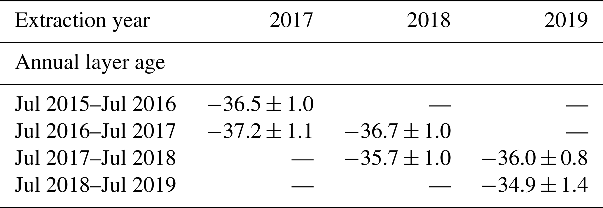
Table B2 Table of changes in δ¹⁸O concentration after 1 or 2 years of aging in the EastGRIP firn from Fig. 7d and c, respectively. Columns are mean annual residuals, summer residuals (June/July), and non-summer residuals. Rows are the years between which the change is calculated. Units are in per mille (‰), and uncertainty is 2${\mathit{\sigma }}_{\stackrel{\mathrm{‾}}{x}}$.

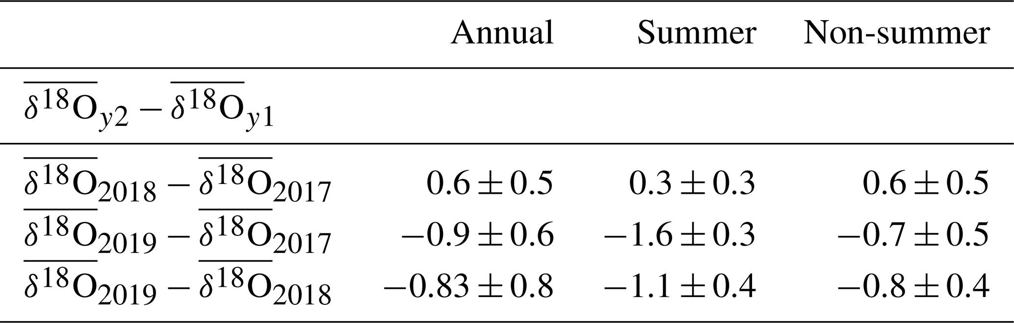
Table B3 Table of annual statistics for d from the EastGRIP snow profiles shown in Fig. 7. Columns are the year of extraction, e.g., “2019” represents the black curve in Fig. 8. Rows are the age of the snow. The annual cycle is winter-centric and computed from 31 July to 31 July. Units are in per mille (‰), and uncertainty is 2${\mathit{\sigma }}_{\stackrel{\mathrm{‾}}{x}}$.

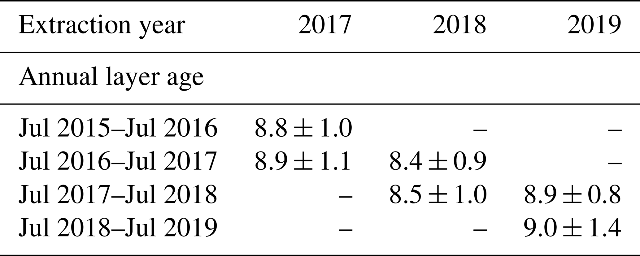
Table B4 Table of changes in d concentration after 1 or 2 years of aging the EastGRIP firn from Fig. 8a and c, respectively. Columns are mean annual residuals, summer residuals (June/July), and non-summer residuals. Rows are the years between which the change is calculated. Units are in per mille (‰), and uncertainty is 2${\mathit{\sigma }}_{\stackrel{\mathrm{‾}}{x}}$.

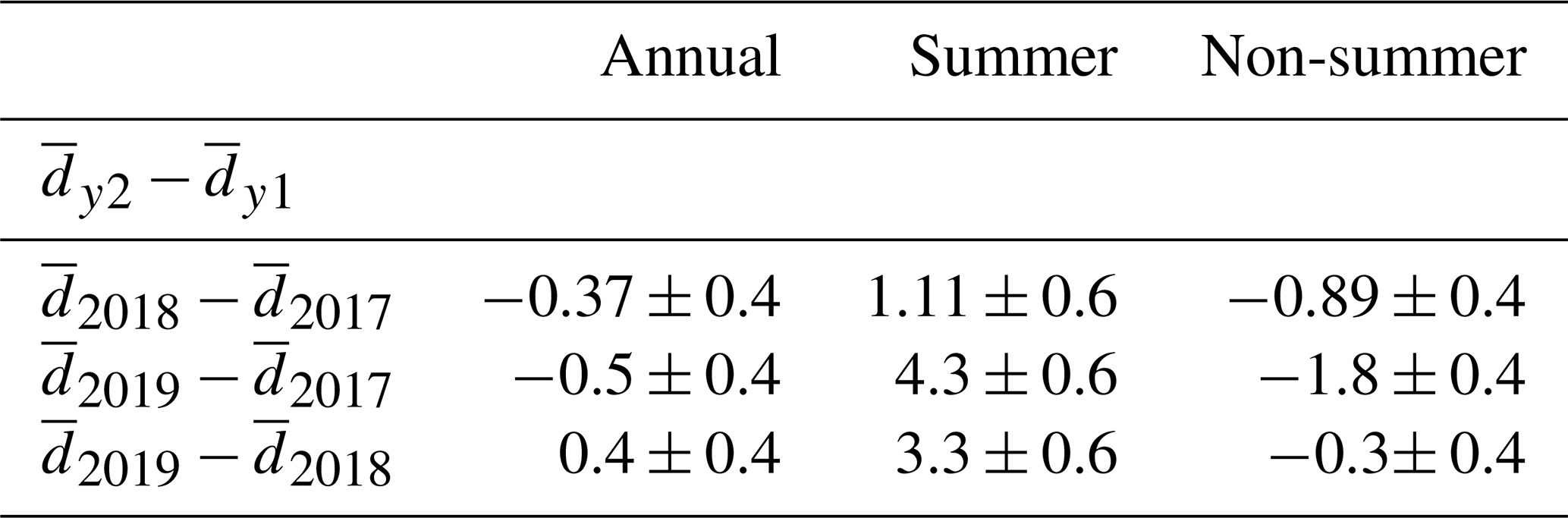
Table B5 Table of statistics for δ¹⁸O and d from the EastGRIP surface snow and d from near-surface summer snow less than 1 year old, as shown in Figs. 7 and 8. Columns are the isotopologues. Rows are the sampling time period. Units are in per mille (‰), and uncertainty is 2${\mathit{\sigma }}_{\stackrel{\mathrm{‾}}{x}}$.

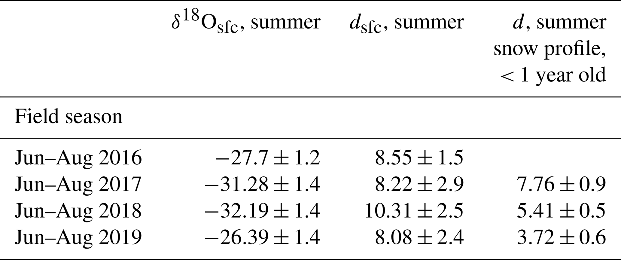
Table B6 Table of δ¹⁸O vs. δD composited by age and season. Summer is June–July. Winter is December–April. Units are in per mille divided by per mille (‰/‰), and uncertainty is 2σ.

Appendix C: Seasonal isotope-to-temperature sensitivity

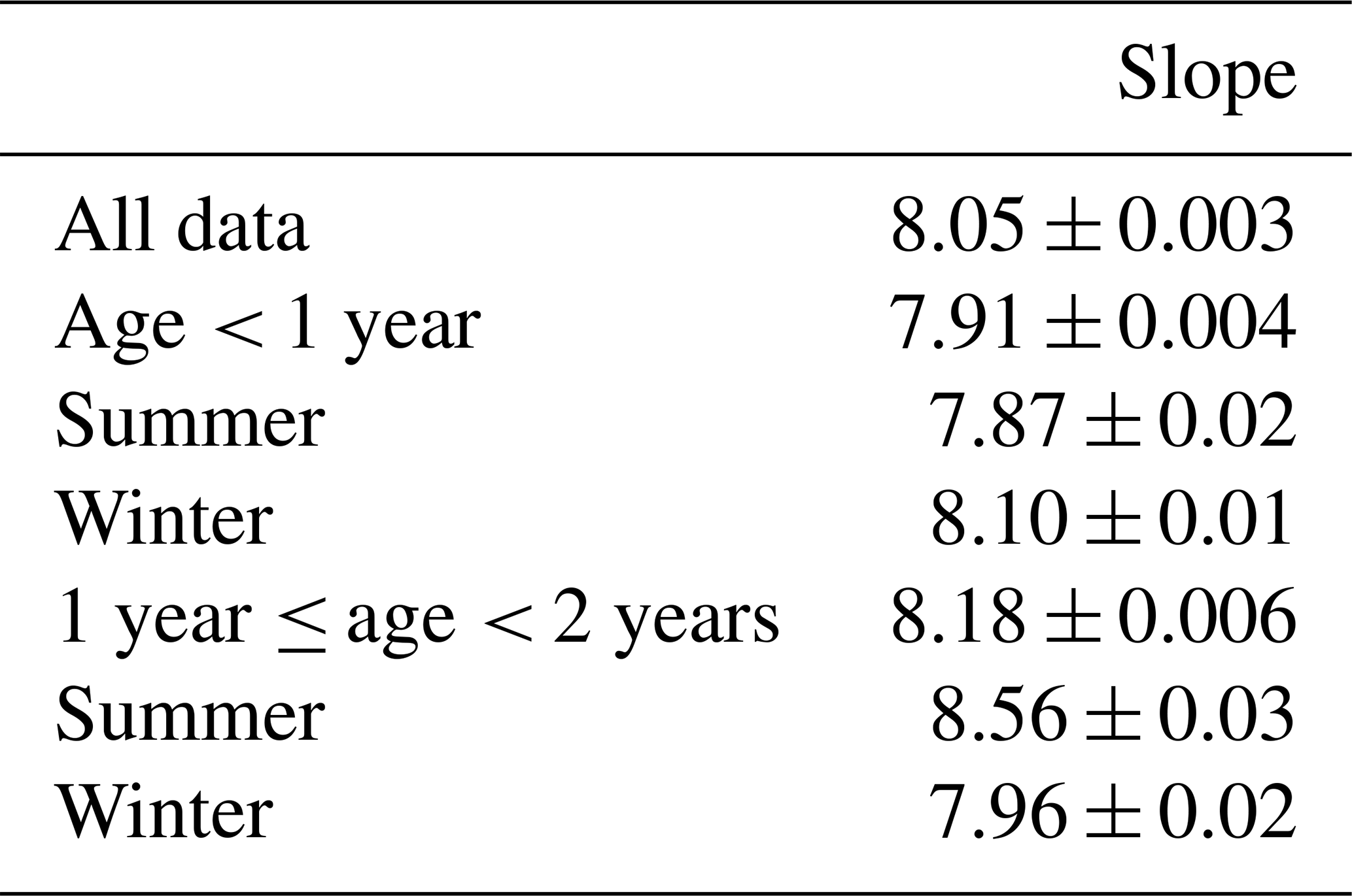
Figure C1 shows the isotope-to-temperature sensitivity as derived from maxima and minima of monthly near-surface temperature and maxima and minima of snow isotopic content.

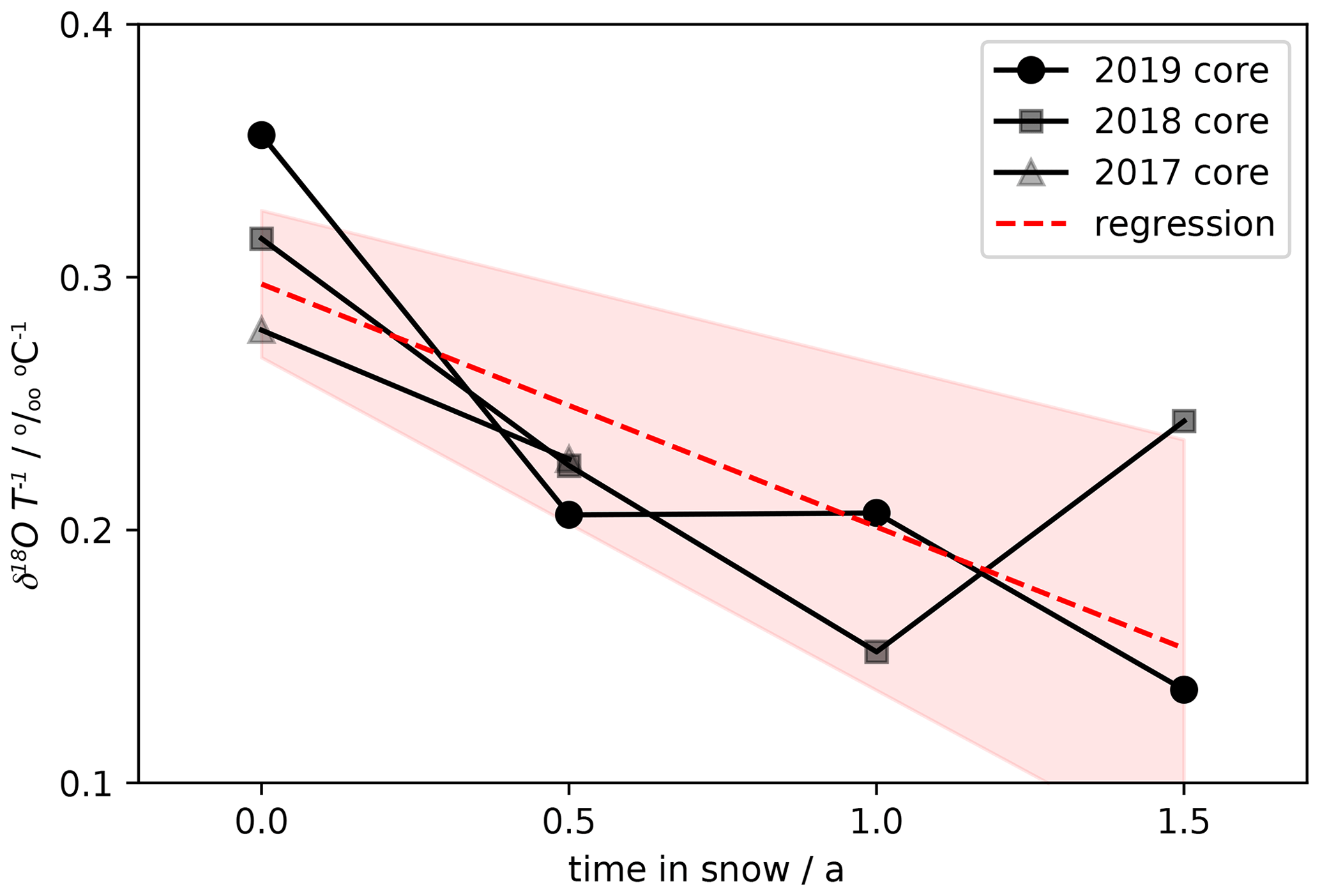
Figure C1 The increase in seasonal isotope-to-temperature sensitivity (γ_t), a decreasing slope, from EastGRIP based on 1.5 years of seasonal maxima and minima in δ¹⁸O and mean monthly temperature. The regression is 2σ and accounts for errors in both variables. Here the line of best fit is Δδ¹⁸OΔT⁻¹ = −0.096 ± 0.036 $\mathrm{‰}\mathrm{°}{\mathrm{C}}^{-\mathrm{1}}{\mathrm{a}}^{-\mathrm{1}}$ ⋅ (time in snow) + 0.297 ± 0.029 ‰ °C⁻¹.

Appendix D: Supporting simulations

D1 Isotope-gradient-driven diffusion simulation scenario

Johnsen et al. (2000) isotopic-gradient-driven (IGD) diffusion is used to explain the pattern and magnitude of the changes we observe in the near-surface snow at EastGRIP. The model is run on the mean δ¹⁸O and δD profiles from the 2019 field season using the following scenario that roughly approximates the annual cycle at EastGRIP: summer is 60 d with snow at −11 °C, autumn is 60 d with snow at −28.5 °C, winter is 180 d with snow at −40 °C, and spring is 60 d with snow at −28.5 °C. This scenario is realistic but may slightly overestimate the amount of diffusion due to the long warm summer used. Sensitivity tests find that applying the diffusion simulations to smoother mean profiles as opposed to individual profiles with sharper features underestimates the amount of IGD diffusion.

D2 Forced ventilation of near-surface snow simulation scenarios

Forced ventilation is simulated based on the snow and atmospheric conditions for the summer season at EastGRIP using an augmented version of Town et al. (2008b). We have added kinetic fractionation (Jouzel and Merlivat, 1984), fractionation on sublimation, and δD to the model. The snow surface structure in the model is parameterized as rolling undulations as prescribed by Colbeck (1997), using peak-to-peak lengths of 1 m and half-heights of 0.1 m, which reflect summertime observations from EastGRIP (Zuhr et al., 2021b, 2023). Snow density is taken from Komuro et al. (2021). The other snow parameters are reasonable assumptions for polar snow (Town et al., 2008b). The summertime isotopic content of atmospheric water vapor over the Greenland Ice Sheet was estimated based on measurements from NEEM (Steen-Larsen et al., 2014) and EastGRIP (Wahl et al., 2022). Note that during these sorts of events the snow surface is dynamic. We do not take this into account in these simulations.

In addition to the two forced-ventilation simulations shown in Fig. 9, additional simulations were performed using the same pairs of snow–air isotope and temperature contrasts to assess the isotopic impact of forced ventilation on near-surface snow. Figure D1 uses wind speeds of 10 m s⁻¹, a typical cyclonic event over EastGRIP that may last 3 d. Figure D2 uses wind speeds of 20 m s⁻¹, a strong cyclonic event at EastGRIP that may last 24 h.

Figure D3 uses the same conditions as shown in Fig. 9, but all fractionation is at equilibrium. Note that equilibrium fractionation ought to result in no change in d, but that does not occur in our simulation because of the definition of d used here (Dütsch et al., 2017). The resulting changes in d are small, only a few per mille, and do not impact conclusions based on the forced-ventilation simulations shown in Fig. 9.

Table D1 Assumptions and driving conditions behind the idealized modeling isotopic evolution of near-surface snow due to forced ventilation.

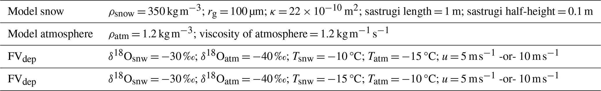
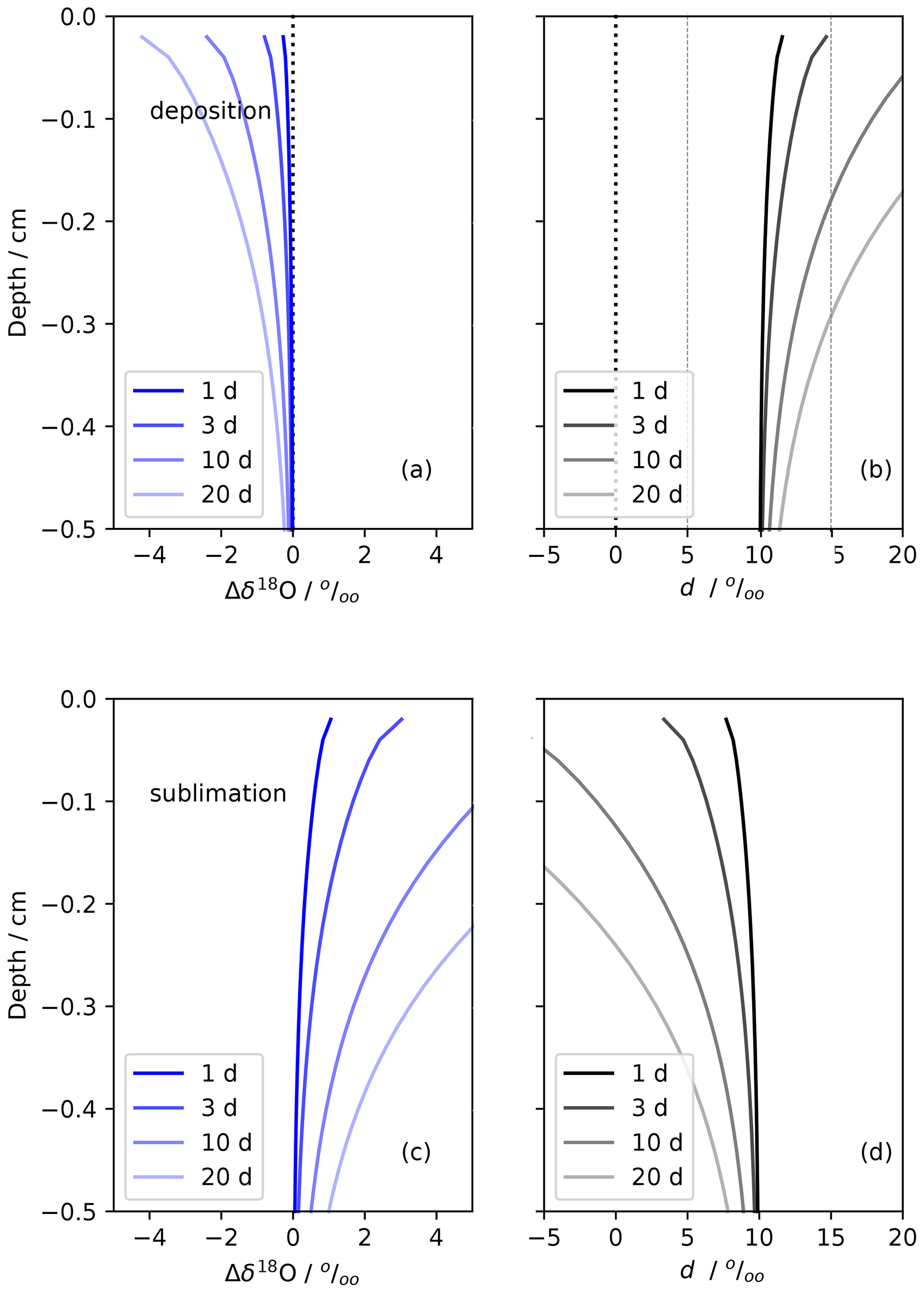
Figure D1 Idealized simulations of forced ventilation on isotropic snow under typical EastGRIP summertime conditions. Panels (a) and (b) show deposition for δ¹⁸O and d, respectively. The deposition conditions are FV_dep, T_snw = −15 °C, T_atm = −10 °C, and u = 10 m s⁻¹. Panels (c) and (d) show sublimation for δ¹⁸O and d, respectively. The sublimation conditions are FV_sub, T_snw = −10 °C, T_atm = −15 °C, and u = 10 m s⁻¹. The snow structure and isotopic content of snow and vapor are detailed in Table D1. This simulation assumes kinetic fractionation.

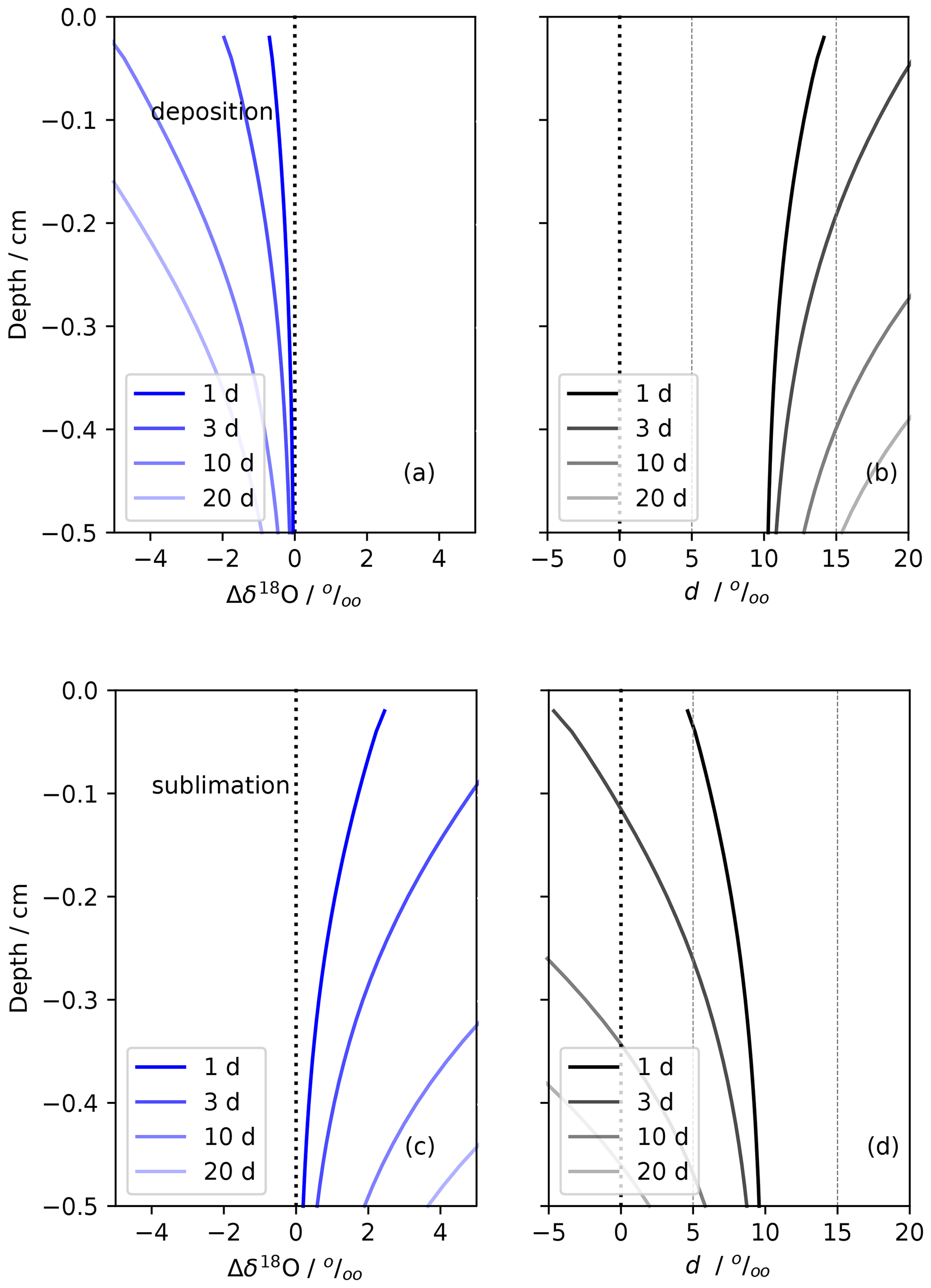
Figure D2 Idealized simulations of forced ventilation on isotropic snow under typical EastGRIP summertime conditions. Panels (a) and (b) show deposition for δ¹⁸O and d, respectively. The deposition conditions are FV_dep, T_snw = −15 °C, T_atm = −10 °C, and u = 20 m s⁻¹. Panels (c) and (d) show sublimation for δ¹⁸O and d, respectively. The sublimation conditions are FV_sub, T_snw = −10 °C, T_atm = −15 °C, and u = 20 m s⁻¹. The snow structure and isotopic content of snow and vapor are detailed in Table D1. This simulation assumes kinetic fractionation.

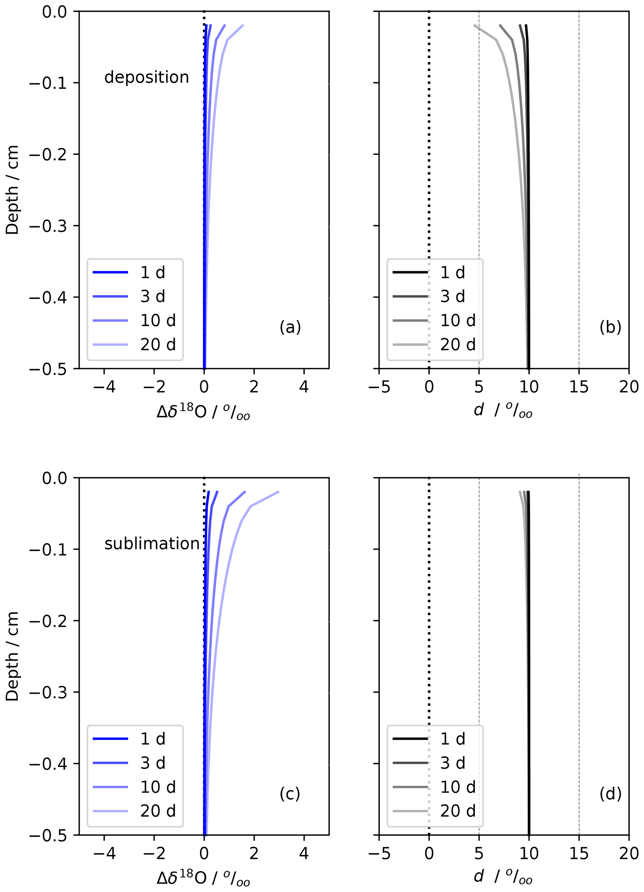
Figure D3 Idealized simulations of forced ventilation on isotropic snow under typical EastGRIP summertime conditions. Panels (a) and (b) show deposition for δ¹⁸O and d, respectively. The deposition conditions are FV_dep, T_snw = −15 °C, T_atm = −10 °C, and u = 5 m s⁻¹. Panels (c) and (d) show sublimation for δ¹⁸O and d, respectively. The sublimation conditions are FV_sub, T_snw = −10 °C, T_atm = −15 °C, and u = 5 m s⁻¹. The snow structure and isotopic content of snow and vapor are detailed in Table D1. This simulation assumes equilibrium fractionation.