the Creative Commons Attribution 4.0 License.
the Creative Commons Attribution 4.0 License.
 | 23 Jul 2024
Measuring prairie snow water equivalent with combined UAV-borne gamma spectrometry and lidar
Warren D. Helgason
John W. Pomeroy
Despite decades of effort, there remains an inability to measure snow water equivalent (SWE) at high spatial resolutions using remote sensing. Passive gamma ray spectrometry is one of the only well-established methods to reliably remotely sense SWE, but airborne applications to date have been limited to observing kilometre-scale areal averages. Noting the increasing capabilities of unoccupied aerial vehicles (UAVs) and miniaturization of passive gamma ray spectrometers, this study tested the ability of a UAV-borne gamma spectrometer and concomitant UAV-borne lidar to quantify the spatial variability of SWE at high spatial resolutions. Gamma and lidar observations from a UAV (UAV-gamma and UAV-lidar) were collected over two seasons from shallow, wind-blown, prairie snowpacks in Saskatchewan, Canada, with validation data collected from manual snow depth and density observations. A fine-resolution (0.25 m) reference dataset of SWE, to test UAV-gamma methods, was developed from UAV-lidar snow depth and snow survey snow density observations. The ability of UAV-gamma to resolve the areal average and spatial variability of SWE was promising with appropriate flight characteristics. Survey flights flown at a velocity of 5 m s−1, altitude of 15 m, and line spacing of 15 m were unable to capture the average or spatial variability of SWE within the uncertainty of the reference dataset. Slower, lower, and denser flight lines at a velocity of 4 m s−1, altitude of 8 m, and line spacing of 8 m were able to successfully observe areal average SWE and its variability at spatial resolutions greater than 22.5 m. Using a combination of UAV-based gamma SWE and UAV-based lidar snow depth improved the spatial representation of SWE substantially and permitted estimation of SWE at a spatial resolution 0.25 m with a ± 14.3 mm error relative to the reference SWE dataset. UAV-borne gamma spectrometry to estimate SWE is a promising and novel technique that has the potential to improve the measurement of shallow prairie snowpacks, and when combined with UAV-borne lidar snow depths, can provide fine-resolution, high-accuracy estimates of prairie SWE. Research on optimal hardware, data processing, and interpolation techniques is called for to further improve this remote sensing product and explore its application in other environments.
- Article
(6234 KB) - Full-text XML
- BibTeX
- EndNote


Snow is a defining feature of the hydrological cycle in cold regions and has significant socioeconomic and environmental implications (Pomeroy and Goodison, 1997; King et al., 2008). A basic and persistent challenge for snow hydrology is efficiently and accurately quantifying snow water equivalent. The overlapping variability of landscape, weather and climate, and snow processes combine to drive significant spatiotemporal differences in snowpack characteristics (Pomeroy and Gray, 1995; Essery and Pomeroy, 2004b; Grünewald et al., 2010; Trujillo et al., 2007; Liston and Sturm, 1998; Shook and Gray, 1996) A significant body of research has been devoted to developing protocols and technologies to observe snow characteristics to inform scientific understandings and decision-making (Kinar and Pomeroy, 2015). Quantifying the spatial variance of snow water equivalent (SWE) allows for calculation of snow-covered area (SCA) depletion during the melt period (Essery and Pomeroy, 2004a; Faria et al., 2000; DeBeer and Pomeroy, 2010), and in turn the SCA depletion is critical to estimate the contributing area, and duration, of runoff and infiltration from snowmelt (Shook et al., 1993; DeBeer and Pomeroy, 2010). To date, the ability to directly and remotely observe the spatial variability of SWE at the fine scales corresponding to the snow redistribution and ablation processes defining snowpack formation has remained elusive (Tedesco et al., 2015).
The SWE (water equivalent water depth per unit area) of a snowpack is expressed in millimetres of water equivalent or kg m−2. Snow surveys of depth (hs) and density (ρsnow) observations along a linear transect are the traditional approach used to calculate SWE and remain the most reliable technique but are a time-consuming, labour-intensive, and ultimately destructive sampling technique (Kinar and Pomeroy, 2015). Non-contact point-scale observations such as snow pillows, passive radiometric sensors, and acoustic sensors have demonstrated success but do not capture spatial variability (Coles et al., 1985; Kinar and Pomeroy, 2007, 2015; Wright et al., 2011). Remote sensing has had great success in quantifying the spatial variability of hs over wide ranges in extent and resolution ranging from satellite stereography (Marti et al., 2016), lidar (aeroplane-borne or UAV-based (UAV-lidar)) (Harder et al., 2020; Jacobs et al., 2021; Deems et al., 2013; Hopkinson and Collins, 2009), and structure-from-motion techniques (Harder et al., 2016; Bühler et al., 2016; Walker et al., 2021). Snow depth observations alone capture a significant amount of the snowpack variability but need additional observations, or estimation, of ρsnow in order to quantify SWE (Painter et al., 2016). SWE remote sensing products tend to be coarse-scale, utilizing passive microwave or gamma remote sensing (Tuttle et al., 2018; Tong et al., 2010; Tedesco et al., 2015) or active radar sensors (Tsang et al., 2021) .
Gamma remote sensing of SWE relies on two principles. First, all soils contain naturally occurring gamma-particle-emitting radioisotope elements (Topp, 1970). Second, mass, including all phases of water, attenuates gamma radiation (Peck et al., 1971). Beer's law, which relates the transmission of radiation through a medium (I) to the intensity of the source (I0) as an exponential function of the attenuation coefficient (μ) and thickness (d) of the attenuating medium, as
can be adapted to estimate SWE from observations of gamma emissions over time. Using count rates of gamma particles above a surface when it is snow-covered (Csnow) and snow-free (Cbare) in place of I and I0, respectively, and assuming a μ for water (5.835 × 10⁻³ mm−1, Carroll, 2001), the d can be interpreted, and solved for, as SWE (mm) as
This requires an assumption of isotropic gamma emissions from the soil and no change in soil water content in the time between the bare and snow-covered surface observations that would change Cbare (Carroll and Carroll, 1989). Two main limitations are inherent in quantifying SWE with gamma approaches. The first is that high attenuation of gamma rays by water leads to complete attenuation of the gamma signal in large snowpacks, such that this technique is limited to medium or shallow snowpacks. In a point-scale/stationary implementation, the Campbell Scientific CS725 passive gamma radiation sensor (Wright et al., 2011; Kinar and Pomeroy, 2015) when fixed above a snowpack can estimate SWE for footprints of 50–100 m2 at 3 m sensor height with 15 % accuracy and is limited to snowpacks with < 600 mm SWE. The CS725 has been shown to work well for uniform and relatively deep mountain snowpacks, if placed on mild slopes where snowmelt runs off instead of ponding (Smith et al., 2017). In an airborne implementation, the NOAA Airborne Snow Survey program has utilized gamma spectrometry to observe peak SWE over much the Red River basin of the north-central US Great Plains and southern Canadian Prairies to inform flood predictions since 1980 (Cho et al., 2019). This airborne program typically employs flight lines at 150 m altitude, 16 km long to provide SWE estimates with approximately 5–7 km2 footprints with errors less than 10 % for snowpacks < 300 mm SWE (Cho et al., 2019; Carroll and Carroll, 1989; Tuttle et al., 2018). The second limitation is that variability in soil moisture is a significant source of uncertainty. A snow-free observation to capture the background gamma state as near as possible to freeze-up is required. In the case of an overwinter increase in near-surface soil moisture, due to snowmelt or rainfall infiltration, end-of-winter SWE will be biased high (Carroll and Carroll, 1989). Approaches to correct for overwinter changes require independent estimates of soil moisture change (Offenbacher and Colbeck, 1991; Carroll, 2001; Carroll and Carroll, 1989), and recent applications have included independent data sources such as SMAP soil moisture (Cho et al., 2020).
Table 1Summary of sites and observations.
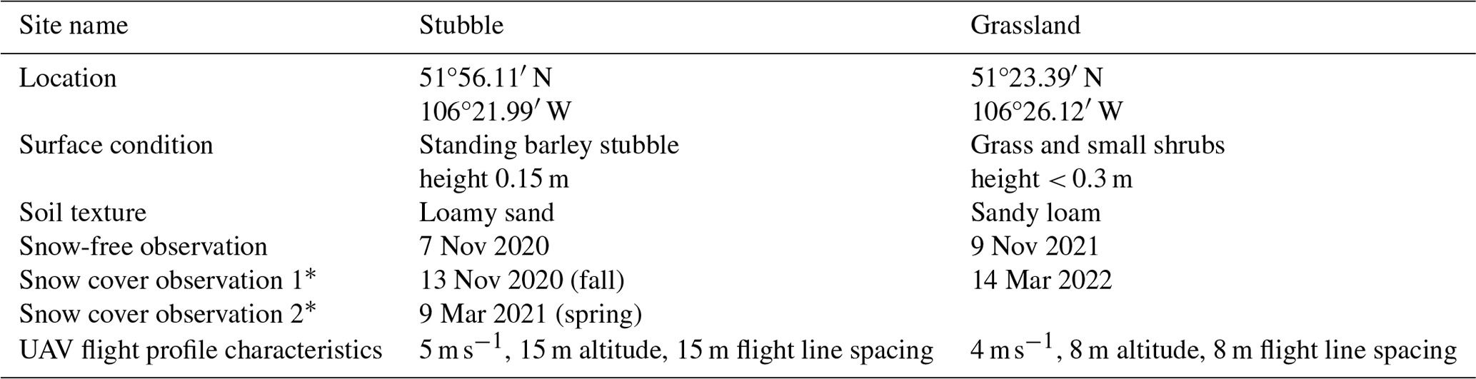
* Bracketed identifiers denote the specific observation for reference hereafter.
Passive radiometric observation methods are sensitive to an integration time and, in mobile applications, challenged by small signal-to-noise ratios (Reinhardt and Herrmann, 2019; Peck et al., 1971). The ability to resolve a feature of interest with gamma spectrometry is directly related to the volume of the scintillation crystal, integration time, and proximity to the target which all need to be balanced by the physical limitations and operational characteristics of the platform, area of interest, and ability to precisely collocate sensors between different surveys (Reinhardt and Herrmann, 2019). The confluence of ever-increasing UAV capabilities (endurance, payloads, and spatial accuracy of navigation) and miniaturization of gamma ray spectrometers has opened the door to UAV-borne gamma spectrometry (UAV-gamma). Most UAV-gamma applications to date have focussed on mapping radiative properties for mineral exploration (Martin et al., 2020) and relationships to soil properties such as texture, type, nutrient status, erosion, organic matter and pH (Reinhardt and Herrmann, 2019). A significant advantage of UAV platforms over traditional crewed aircraft is the ability to repeatedly fly consistent flight lines at low altitudes and speeds.
The ability of UAV-borne gamma spectrometry to quantify SWE has not been reported in the scientific literature, nor has the possibility to interface gamma-measured SWE with fine-resolution snow depth observations from UAV-lidar been examined. The purpose of this work is to demonstrate the workflows needed for deploying UAV-borne gamma spectrometry over snow and then to evaluate the following: (1) the ability of UAV-borne passive gamma spectrometry to directly observe the SWE of shallow agricultural snowpacks and (2) the potential for UAV-borne gamma spectrometry by itself, and combined with UAV-lidar, to estimate the spatial variability of SWE at fine spatial scales.
2.1 Study area
Observations were collected over two snow seasons between fall 2020 and spring 2022 southeast of Saskatoon, Saskatchewan, Canada, in an agricultural region of the Canadian Prairie ecozone. Two study sites were chosen, both of which have low relief and hummocky topography (Table 1). The stubble site is a cultivated field, seeded the previous year with barley that was harvested in September, leaving a 15 cm standing stubble. The perennial grassland, which is grazed during summer, contained grasses, fescues, shrubs, and forbs with a height ≤ 30 cm in fall 2021. As a result of drought conditions in summer/fall, field observations showed low near-surface soil moisture contents at both sites and dampened spatial variability in both years. The snow season is typically 4–5 months in duration, and on average 30 % of precipitation falls as snow (Pomeroy et al., 2007) . The regional hydrometeorology is extremely variable, and peak SWE can vary from negligible in dry years to > 100 mm in cold and snowy winters (Pomeroy et al., 2007).
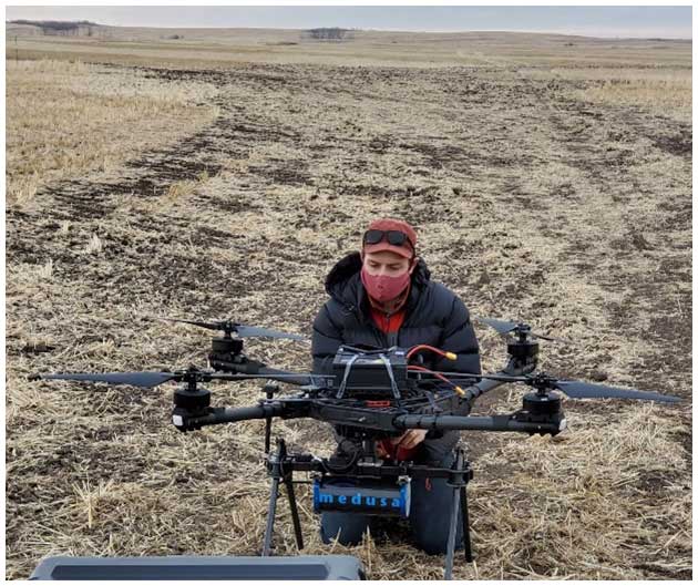
Figure 1Medusa MS-1000 mounted on a FreeFly AltaX prior to survey 6 November 2020. Photo credit: Anders Hunter.
2.2 Data collection
2.2.1 Site conditions and surveys
Several UAV gamma surveys were made, concomitant with UAV-lidar surveys. Meteorological conditions during the respective seasons were observed using well-instrumented meteorological stations (part of the Global Water Futures Observatories http://www.gwfo.ca, last access: 7 July 2024) near the study locations. Each survey captured different environmental and deployment conditions. In fall 2020, a bare ground survey was conducted at the stubble site on 6 November immediately preceding 60 mm of SWE which fell over 7–9 November. This provided an opportunity to test the SWE estimation by conducting a subsequent snow-covered survey on 13 November. For this survey interval, there was a clear transition between exposed, unfrozen, and relatively dry soil conditions to a continuous snow cover and frozen soil in the near surface. The weather after the snowfall event was consistently cold, with no snowmelt or rainfall, so soil moisture was static, and the only change in gamma ray attenuation can be attributed to the accumulation of a snowpack. Wind redistribution of snow was a function of topography with transport from flat and wind exposed ridges and northwest-facing slopes to deposition locations in relatively wind sheltered locations on southeast-facing slopes. Development of transverse dunes (Filhol and Sturm, 2015) in wind-exposed locations also provided an increase in small-scale SWE spatial variability. In contrast, the spring survey at this site, with exactly the same flight profile as in the fall survey, observed end-of-winter conditions and thus represents the accumulation and wind redistribution of several snowfall events over the winter, resulting in a generally deeper snowpack on southeast facing lee slopes with greater spatial variability in flat areas with development of transverse, sastrugi, and barchan dune snowdrifts (Filhol and Sturm, 2015). For the second season, the grassland site was surveyed at a lower altitude and slower flight speed, with denser flight line spacing. The grassland site had greater SWE than that observed in the stubble field surveys, and spatial variability was primarily due to relatively large snowdrift formation in the lee of fences. There was a positive relationship between vegetation height and snow depth, and taller vegetation suppressed the formation of snowdrift dunes. A significant mid-winter melt event took place from 7–10 February 2022, with maximum air temperatures reaching 6 °C and a 15 cm decrease in snow depth observed at a GWFO meteorological station 10 km from the study site. Snow cover remained continuous, and meltwater flow through the snowpack and refreezing as a spatially discontinuous basal ice lens were observed during snow surveys.
2.2.2 Gamma observations
Gamma emissions were observed with a Medusa Radiometrics MS-1000 passive gamma ray spectrometer mounted on a Freefly AltaX UAV platform (Fig. 1). Flight planning and control was done with ALTA_QGroundControl software. Flight navigation used regular GPS signal for stubble surveys (± 5 m positioning), while navigation for grassland flights used an updated RTK system (centimetre-level positioning). The MS-1000 utilized a 1 s integration time for gamma emissions and observed GPS, air temperature, humidity, and air pressure information with an integrated sensor.
In airborne applications with the spectrometer offset from the surface, airborne corrections are often implemented in order to account for the interactions of gamma rays in the air mass as well as to correct for radon and cosmic ray emissions that share this part of the electromagnetic spectrum. The Gamman software included with the MS-1000 by Medusa Radiometrics provides tools for airborne corrections with a full spectrum analysis approach. As flights were ≤ 15 m above the ground surface, where airborne corrections do not make a significant difference compared to the uncertainty introduced, no airborne corrections were applied based on advice of the manufacturer. Gamman (Medusa Radiometrics, 2024) was used to perform energy stabilization of the spectra and generate count rates (C) and corresponding latitude, longitude, and height data at 1 s intervals. Gamman employs a proprietary full spectrum analysis to fit a “standard spectra” to the measured spectrum, with the fitting factors quantifying the radionuclide concentrations (Hendriks et al., 2001). To account for detector and environmental drive factors, Gamman employs a stabilization algorithm to align the measured spectra to the corresponding gamma energy. Total count rates are quantified from the integration of the stabilized and aligned spectrum. Due to data gaps in MS-1000 GPS data, the AltaX flight telemetry was used to resolve sensor trajectory. Manual alignment of the telemetry and MS-1000 GPS data was needed due to timestamp mismatches. Precision of the GPS data accessible from the AltaX telemetry logs was degraded despite RTK navigation, so a 13-point rolling average was used to smooth the positioning data. The 13-point rolling average was a compromise between increased precision and alignment with the known flight path. All data at the ends of the flight lines associated with platform slowing and turning waypoints were removed with spatial clipping to ensure that count rate observations represented consistent flight speeds and footprint characteristics. An example of the raw count data and positioning is visualized in Appendix A.
2.2.3 Validation data
A reference dataset of SWE (SWEref) was developed from UAV-lidar hs and snow survey ρsnow observations. UAV-lidar surveys quantified the spatial variability of hs at a 0.25 m spatial resolution. A Freefly AltaX UAV platform with a Riegl miniVUX2-UAV lidar was flown over the extent of the snow-covered survey areas on the same day as gamma flights. The data processing workflows to generate digital surface models (DSMs) are detailed in Harder et al. (2020). Utilizing approaches from LAStools (Isenburg, 2019), the irregular lidar point cloud was processed to a 0.25 m gridded representation via a TIN surface fitting approach. Rescaling from the 0.25 m base resolution to other resolutions used the mean value of the larger grids. The hs was computed as the difference between the snow-covered DSM and existing snow-free DSMs of the respective sites. Flights were conducted at an elevation of 110 m, with 80 m between flight lines, at a speed of 10 m s−1. The overall SWEref uncertainty (ΔSWEref: mm) was propagated from the uncertainty of the observed snow density (Δρsnow) and UAV-lidar snow depth observations (Δhs-UAV) as
where i indexes all snow hs-UAV observations between 1 and n (total number of observations). The Δhs-UAV was assumed to be 5 cm, a conservative value for this domain from the literature (Harder et al., 2020; Jacobs et al., 2021). For each flight, manual snow surveys collected between 12 and 60 observations of ρsnow with an ESC-30 snow tube (Pomeroy and Gray, 1995). Survey-specific mean ρsnow was calculated, and its uncertainty (Δρsnow) was estimated via error propagation. Assuming an hs uncertainty (Δhs) of 1.27 cm (ruler had increments of inches) and snow mass uncertainty (Δmass) of 5 % (0.05 ⋅ mass), the uncertainty of individual ρsnow observations was consolidated to a survey scale Δρsnow as
where i indexes the individual ρsnow observations and its constituent terms for the respect surveys.
2.3 Gamma SWE processing
To relate gamma emissions observed from a moving passive sensor to a spatially distributed SWE is a signal-to-noise and interpolation challenge. Two main factors need to be considered: the first being the temporal stability of a gamma observation and the second the footprint it represents. At 1 s integration intervals, and a scintillation crystal volume of 1 L, count rates are often unstable, and, based on the flight profiles employed, each observation will have overlapping footprints in longitudinal and lateral dimensions.
2.3.1 Count rate stability
To understand the temporal stability of this system, C observations were analyzed at start of every flight when the system was static on the ground surface. The mean C for a 75 s interval was assumed to be the true C of the surface. Aggregating the 1 s C with rolling means between 1 and 75 s simulates different integration times. The coefficient of variation (CV) for the difference in integration time mean and the 75 s mean were used to articulate a relationship between signal stability and integration time. This provided a means to estimate the integration period required to establish a stable C.
2.3.2 Spatial representation
A drop-in-the-bucket (DIB) oversampling scheme was used to resolve a gridded product with minimal noise (Long et al., 2019) as common grids are needed to compare observed and estimated SWE and determine errors when varying spatial resolution. Spatial interpolation techniques, such as kriging or spline interpolation, were not implemented in this work to avoid associated biases and artefacts and rather focus on the implications of spatial resolution and number of individual observations aggregated. For DIB, a dense grid was generated for the respective areas of interest, with resolutions ranging between 10 and 50 m at 2.5 m intervals. For each grid resolution the mean C, and number of 1 s integrations included, at each grid point are computed from all points within a radius equivalent to the distance between the centre and corner of the raster pixel. Upon computation of the respective C for the various resolutions, and snow and snow-free situations, the C values were input to Eq. (2) to compute SWE. Henceforth all SWE estimated from gamma observations is denoted as SWEgam. The SWEref was resampled to the respective resolutions to allow for direct comparison with the SWEgam.
2.3.3 Gamma–lidar data fusion
A completely non-contact-UAV-based SWE (SWEgam-lid) was made by fusing fine-resolution hs from lidar data and density from SWEgam. A field-scale mean snow density (ρsnow) was quantified from a field-scale mean gamma SWE () and an independent field-scale mean snow depth () from lidar as
The ρsnow in turn was reapplied to the spatially variable hs from the UAV-lidar to estimate spatially distributed SWEgam-lid as
3.1 Snow density uncertainty
The uncertainty of SWEref comprised observational errors associated with density and depth observations. For the respective manual snow surveys, the mean ρsnow and uncertainty was summarized in Table 2. No meaningful relationships between hs–ρsnow (Fig. 1) were observed, so survey average values of ρsnow are deemed to be appropriate.
Table 2Snow density mean and uncertainty from Eq. (4) for respective snow surveys.

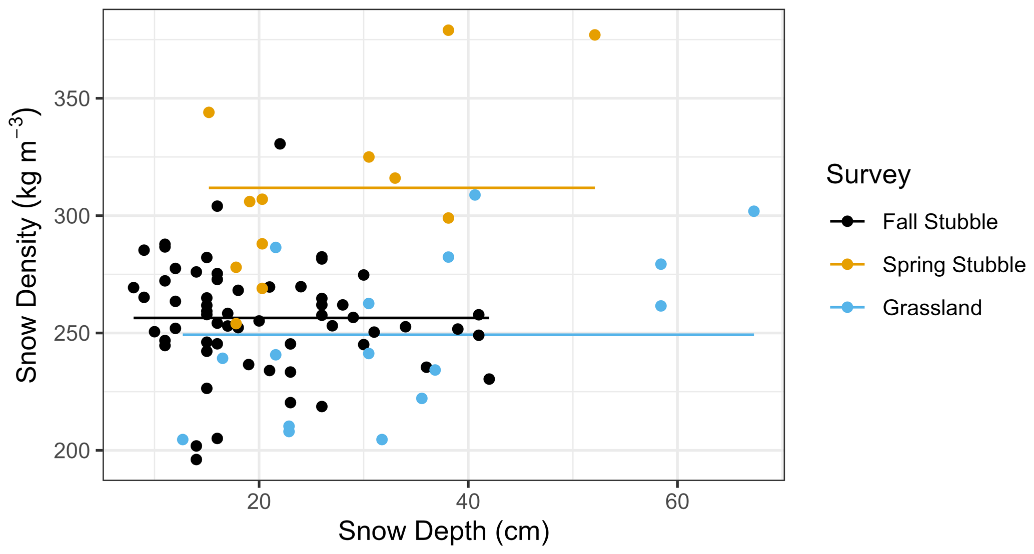
Figure 2Manual snow survey density (kg m−3) versus snow depth (cm) observations (top), with the mean value (horizontal solid line) for respective surveys (colour).
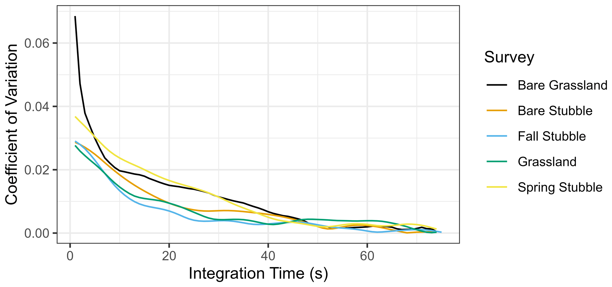
Figure 3Total count coefficient of variation for static operation, prior to all survey flights, of the UAV passive gamma ray spectrometer with varying integration time.
3.2 Count rate stability
Stable count rates are needed to ensure confidence that meaningful observations are being collected. For this, the primary factor, specific to the volume of the scintillation crystal, was the integration time. Operating the spectrometer on the ground prior to takeoff demonstrated the influence of integration time (Fig. 3). By varying the integration time with application of different rolling mean windows, it was evident that the coefficient of variation (CV) decreases logarithmically with integration time, while mean bias was relatively stable. The longer the integration time, the lower the CV. An inflection point in integration time occurs near 20 s when CV was between 0.01 and 0.02. Longer integration times have a decreasing rate of CV change.
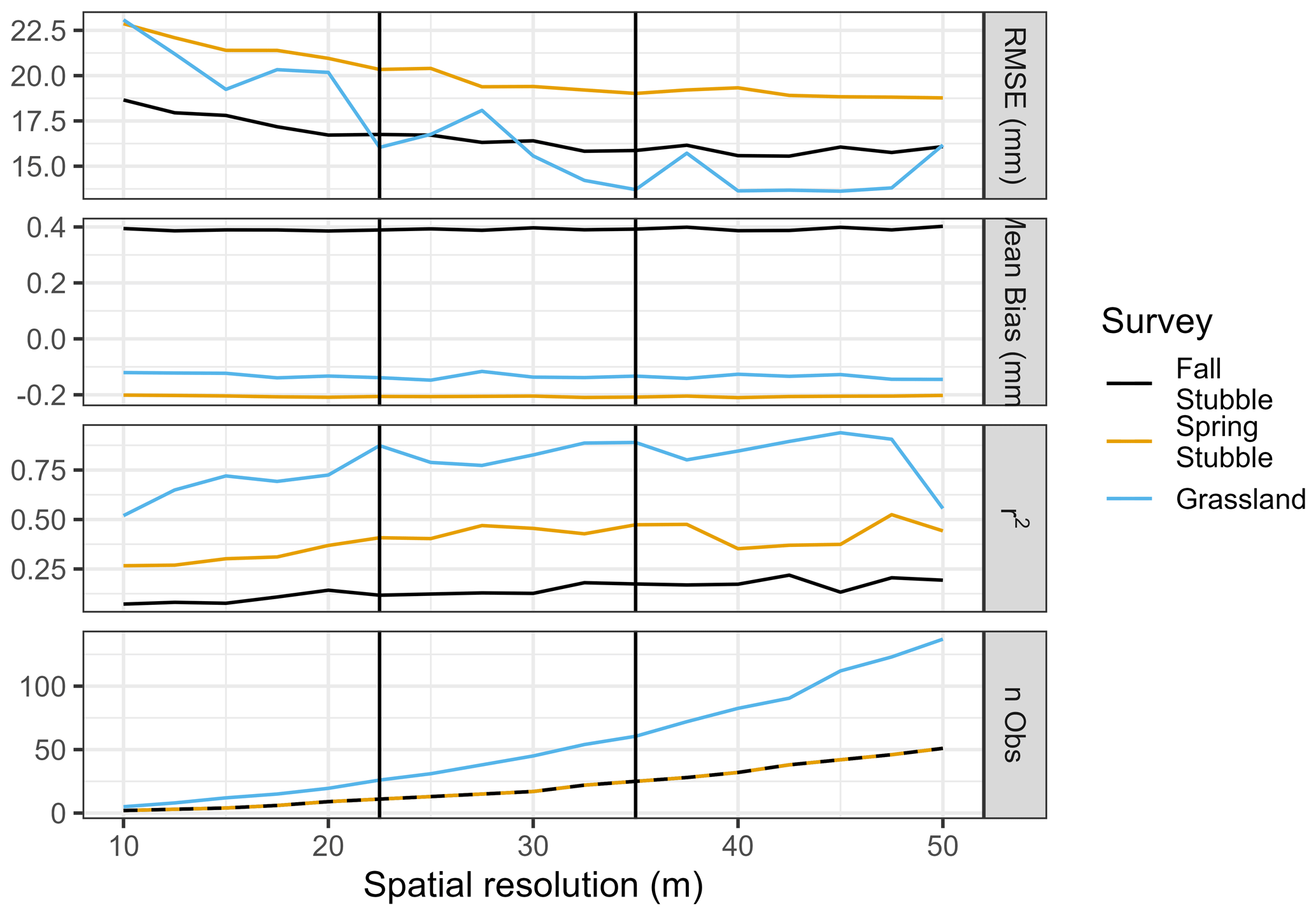
Figure 4The root mean square error (mm: RMSE), mean bias (mm), coefficient of determination (r2), and median number of count rate observations versus raster resolution for all surveys. RMSE, mean bias, and r2 are computed relative to resampled SWEref. The 22.5 and 35 m spatial resolutions are highlighted by the respective vertical black lines.
3.3 Errors versus spatial resolution
The root mean square error (RSME), mean bias, and coefficient of determination (r2) of SWEgam versus the resampled SWEref are shown in Fig. 4. The RMSE and r2 improve as the spatial resolution increases, while the mean bias remains static. An important dynamic was the influence of flight characteristics on survey errors. The surveys conducted at the stubble site, which had higher altitudes, wider line spacing, and higher speed, clearly show higher errors than the slower, lower, and narrow flight spacing of the grassland surveys. The median number of points for each raster cell for the bare and snow-covered surveys is also noted. For grassland surveys, the 22.5 m spatial resolution was associated with approximately 20 gamma observations. In contrast for stubble surveys, a spatial resolution of 35 m is required before the median number of observations reaches a similar 20 observation target. The 22.5 m resolution coincides with an inflection point for the RMSE and r2 metrics for the grassland survey. The RMSE and r2 values decrease between 10 and 22.5 m resolutions, and thereafter the rate of change slows. Variability in the grassland metrics begins to appear at the 22.5 m resolution and was explained by the overall extent of the area increasing and decreasing as pixels progressively increase in size and entire rows/columns on the edges of the extent are dropped progressively.
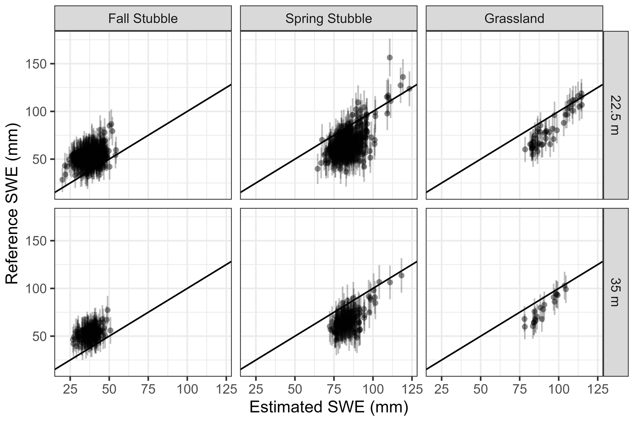
Figure 5UAV-lidar and snow density survey reference versus UAV-gamma-estimated snow water equivalent for 22.5 and 35 m resolutions for respective surveys, with the 1:1 line plotted. Vertical errors bars are the propagated uncertainty of the SWEref.
The scatter plot between the resampled SWEref and SWEgam in Fig. 5 for 22.5 and 35 m resolutions demonstrates the positive and negatives biases of fall and spring stubble surveys, respectively. The grassland relationship was stronger with limited bias in the SWEgam, though the variability was muted relative to the resampled SWEref.
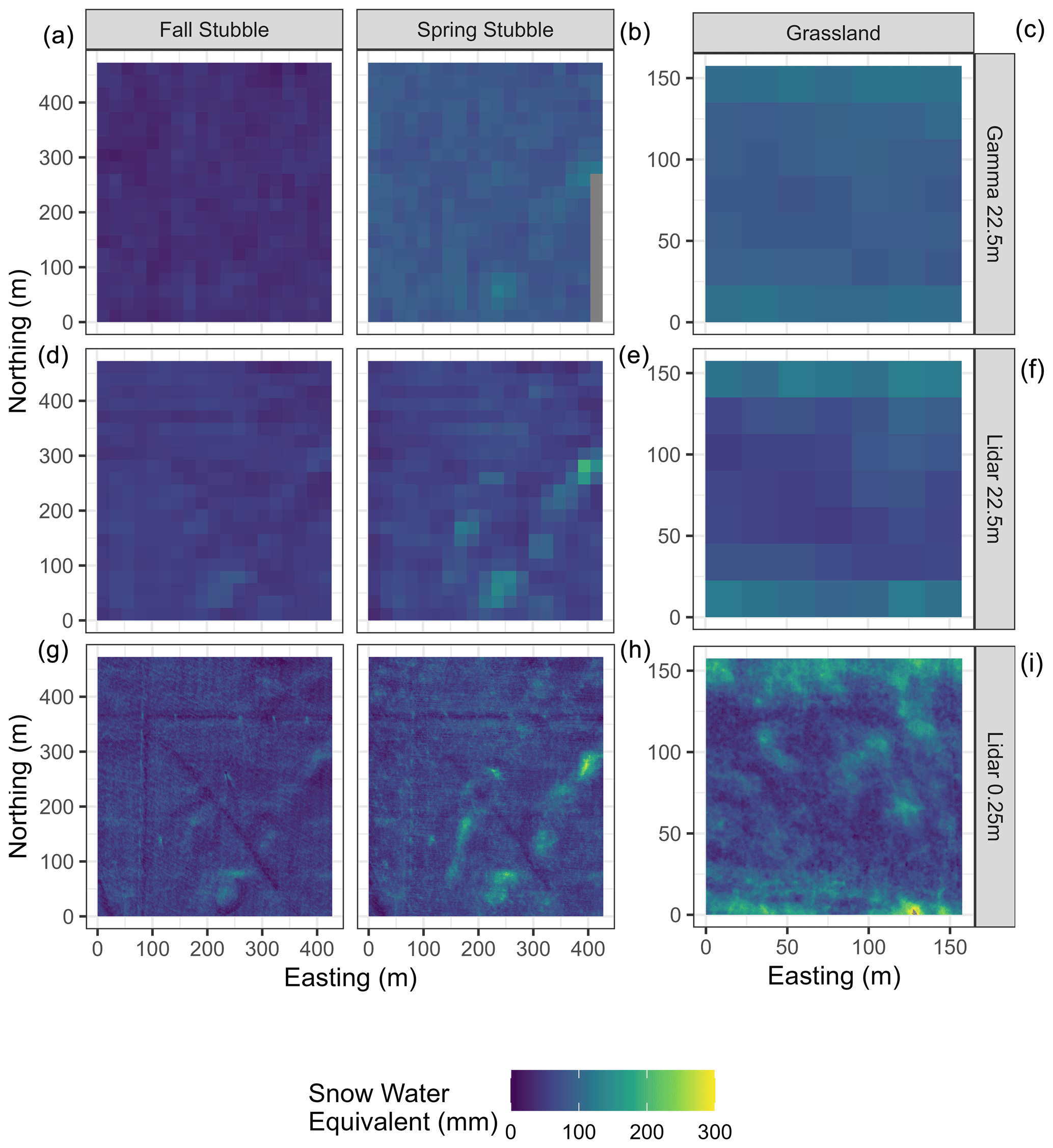
Figure 6Snow water equivalent maps at 22.5 m resolution from the UAV-gamma technique (a–c); 22.5 m resampled UAV-lidar and snow density survey reference, SWEref (d–f); and 0.25 m, SWEref (g–i) for the fall stubble (a, d, g), spring stubble (b, e, h), and grassland (c, f, i) surveys.
Comparisons of the spatial features discernible for the 22.5 m resolution SWEgam and SWEref, and in the original 0.25 m resolution, visualize the ability of the technique to discern SWE features (Fig. 6). The negative bias of the fall stubble SWEgam was evident and with little spatial coherence to the resampled SWEref. While muted and nosier than the resampled SWEref, the diagonal snowdrift features in the southeast of the domain were captured by the gamma in spring stubble survey. The grassland survey demonstrates the most coherence between the 22.5 m resampled SWEref and SWEgam. The snowdrifts on the north and south are evident as well as increases in SWE in the depressions in the centre of the domain. Overall, the variability of the SWEgam was much more muted than the SWEref.
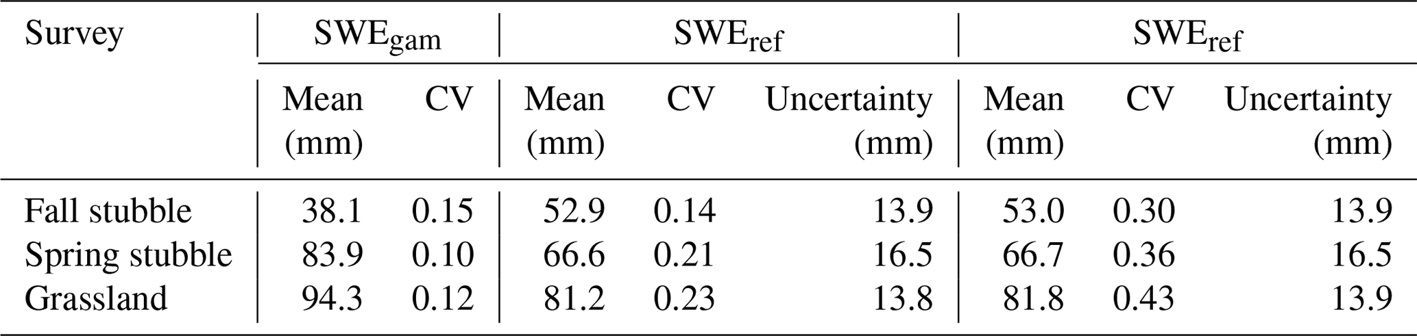
Table 3Snow water equivalent site summary statistics for gamma-based (22.5 m) and lidar-based (22.5 and 0.25 m) resolution SWE.
3.4 Statistical properties of SWE distributions
Statistical properties of the SWE distributions, specifically the mean and CV of SWE for the respective survey areas, were computed from the 22.5 m resolution SWEgam and SWEref, as well as the 0.25 m resolution SWEref (Table 3). The mean SWEref was similar for the 22.5 and 0.25 m resampling as a common survey area was used. The mean SWEs provide coarse-scale metrics analogous to traditional airborne gamma survey metrics. The mean SWEgam for grassland was within the uncertainty bound of the SWEref (from Eq. 3) at 22.5 and 0.25 m resolutions. For fall and spring stubble, the mean SWEgam, except for fall 22.5 m resolution SWEref, was outside of the uncertainty range. The smaller magnitude of SWE, and larger uncertainty, for stubble surveys reduces confidence in these surveys. The CV of the 0.25 m resolution SWEref was the highest of all the surveys (ranging between 0.3 and 0.43). For the resampled 22.5 m SWEref, the CV drops (between 0.14 and 0.29). Other than fall stubble, which had a slighter higher CV for SWEgam at 0.15 versus SWEref at 0.14, the SWEgam was lower than the 22.5 m SWEref, ranging between 0.10 and 0.15.
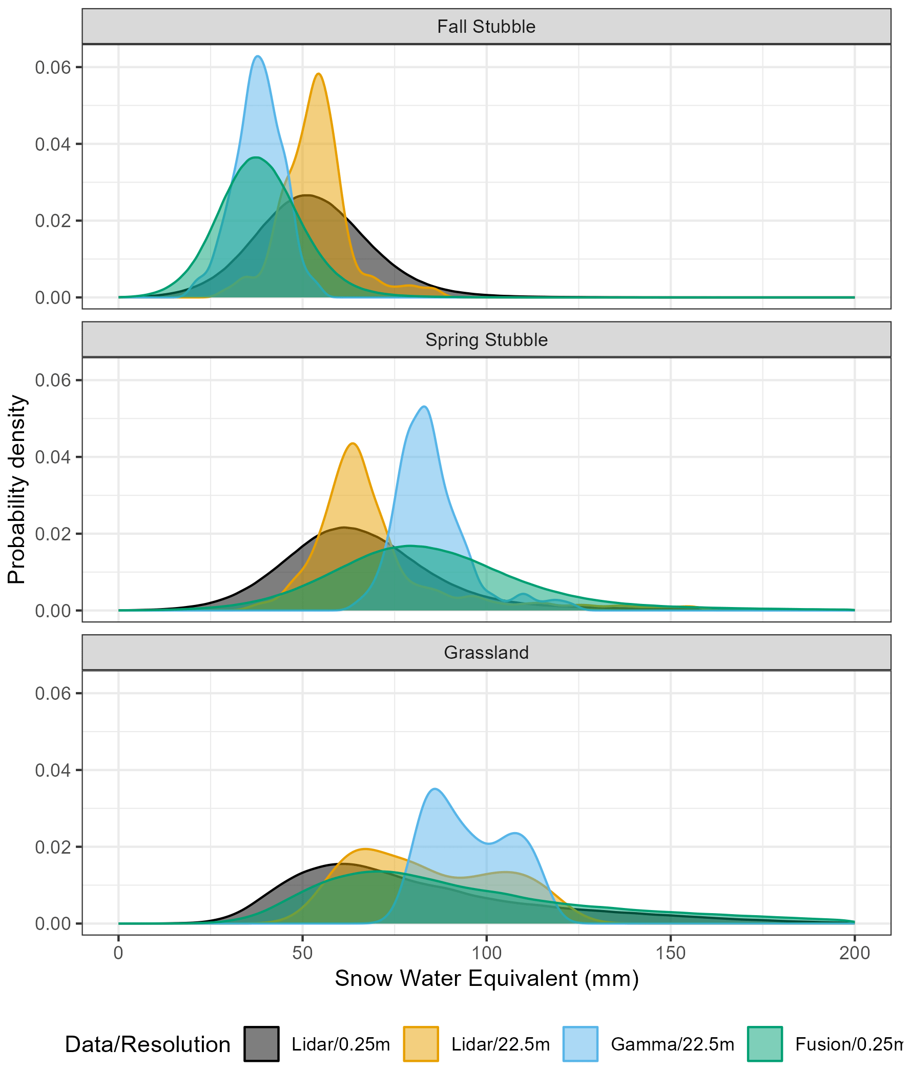
Figure 7Probability density plots of snow water equivalent for the different surveys (rows) and estimation method/resolution (colour).
To compare the statistical distributions of the different SWE representations, density plots are shown in Fig. 7. All 22.5 m resolution data had lower CVs than the 0.25 m resolution and were also lower than the reference distribution. Resampling of the 0.25 m resolution observations to coarser scales meant similar mean values but reduced variability. From Table 3, the CV of 22.5 m SWEref is 53 % of the 0.25 m SWEref. The SWEgam means are higher (grassland +12.5 mm and spring stubble +17.2 mm) or lower (fall stubble −14.9 mm) than the 0.25 m SWEref, with the greatest departures for the stubble sites. Only the grassland SWEgam was within the uncertainty bounds of the corresponding 0.25 m SWEref. Variability of SWEgamwas also lower with the mean CV 34 % of the corresponding 0.25 m SWEref areas. The grassland SWEgam demonstrates greater variability than the stubble surveys. The grassland SWE distribution shows a bimodal distribution that was evident for all resolutions and observation techniques. Regardless of technique utilized, it was apparent that the 22.5 m resolution data struggle to accurately capture the statistical/spatial variability of the 0.25 m SWEref data.
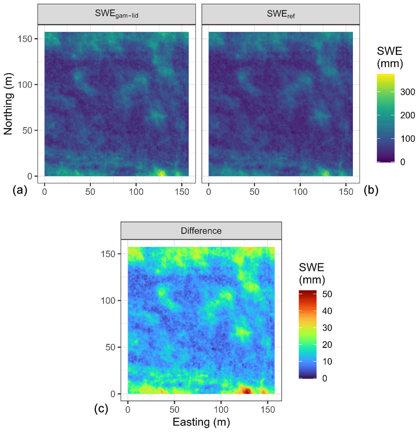
Figure 8Fine-resolution (0.25 m) snow water equivalent (SWE) estimated from UAV-lidar snow depth and UAV-gamma SWE fusion (a) versus reference UAV-lidar and manual snow survey density SWE (b) and their difference (SWEgam-lid − SWEref: c) for the grassland site.
3.5 Fine-resolution SWE from gamma–lidar fusion
Combing lidar-derived hs and SWEgam observations of grassland demonstrates a workflow to estimate SWE at a 0.25 m resolution completely using remote sensing methods that require no manual snow survey (Fig. 8). The average value of SWEgam-lid was 95 mm, while the corresponding SWEref (Table 3) was 82 mm, and the RMSE between the two was 14.3 mm. The difference map in Fig. 8 between SWEref and SWEgam-lid demonstrates that the fusion approach overestimated SWE as a function of snow depth, owing to a constant ρsnow being applied. The probability density plot of the SWEgam-lid (fusion/0.25 m in Fig. 7) demonstrates a very similar distribution to that of the SWEref (lidar/0.25 m in Fig. 7) for the grassland survey versus the fall and spring stubble surveys, which showed biases with respect to the shifted peaks.
4.1 Accuracy, spatial resolution, flight characteristics, and snowpack scaling interactions
Relating the error metrics between spatial resolution and respective flights profiles demonstrates the many challenges of UAV-borne gamma spectrometry to capture SWE spatial variability. Temporally integrating the spectral observations is a common approach to stabilize the gamma signal, and the minimum integration time was identified as an inflection point at 20 s in Fig. 3. Length scales of 10 to 100 m are typically needed to capture the spatial variability of a prairie snow cover, with a +30 m “fractal cutoff” length scale reported to overcome autocorrelation effects on flat, open Canadian Prairie fields (Shook and Gray, 1996). For UAV operations, a 20 s integration time created long and narrow elliptical footprints (i.e., grassland flight footprints were approximately 15 m wide and 95 m long) that exceeded the 30 m fractal cutoff reported for analogous snowfields (Shook and Gray, 1996). To avoid elliptical footprints, a DIB approach to meet the integration threshold was applied that resulted in similar areal extents but circular shapes (grassland flights give approximate footprints with a radius of 21.6 m). The stabilization of the relation between error metrics and resolution occurred at 22.5 and 35 m resolutions for grassland and stubble surveys, respectively, which aligns with the integration time threshold. Error stabilization for grassland at 22.5 m was associated with a 16.0 mm RMSE, −0.14 mm bias, and 0.87 r2. For the 35 m interval stubble surveys, the RMSEs were similar (15.9 and 19.0 mm for fall and spring stubble, respectively), but the larger biases (0.36 and −0.24 mm for fall and spring stubble, respectively) and lower r2 (0.17 and 0.47 for fall and spring stubble, respectively) imply that variability was not being captured as well. While there was a difference in GPS navigation accuracy between the grassland and stubble flights (Sect. 2.2.2), the much larger signal footprint and its high sensitivity to flight altitude negate this as a significant source of error. These interactions demonstrate the scaling challenges of trying to extract spatial information on SWE from UAV-gamma. The slower, lower, and denser flight lines over the grassland reduced the footprints enough to begin to converge on the underlying SWE variability, while stubble flight footprints and SWE variability did not align. The flight characteristics required to meet specific resolution objectives will be sensor-specific and a proposed approach to guide flight planning best practices is articulated in the Appendix B.
4.2 Non-contact fine-resolution SWE with sensor fusion
An ongoing need for snow hydrology is to be able to remotely sense wind-redistributed snowpack SWE at fine resolutions without resorting to supplementary surface observations. The large gamma footprints relative to snowpack-scale variability, as discussed, challenge the use of gamma techniques alone to directly measure SWE spatial variability. Notwithstanding, UAV-borne gamma spectrometry does have value in fusion with fine-resolution snow depth estimates from lidar or possibly other approaches such as UAV-based structure from motion, providing opportunities for this tool to advance remote snowpack measurement and mapping.
The overestimation of SWE can be partly explained by a melt event earlier in the winter. Shallow snow, with less cold content to buffer a positive energy balance and lower liquid-water-holding capacity to absorb snowmelt, experiences relatively greater melt and snowpack outflow than the deeper drifts (Gray and Landine, 1988; Fernández, 1998; Pomeroy et al., 1998). The SWEref was based upon a snow depth derived from a surface difference, and so it will not reliably measure snowpack density changes due to meltwater redistribution and refreezing. In contrast, the SWEgam will still be influenced by the presence of this refrozen water. The complexity of snow mid-winter melt snow processes and the inability to map the accumulation, redistribution, and refreezing of the meltwater non-destructively and independently at the snow–soil interface complicate validation of SWEgam-lid with respect to the depth-based SWEref.
The ability to discriminate between water or ice stored in the snowpack and that which infiltrated or runoff can be important depending upon the research question or application. In shallow snowpacks such as those found in the Canadian Prairies, midwinter melts can be responsible for hydrologically significant changes in the snow and snow–soil interface, and UAV-gamma is not likely to observe changes in SWE in addition to near-surface soil water/ice mass. This creates challenges in situations where SWE estimates are important but also creates opportunities. For instance, quantifying the total water change in the snow and near-surface water/ice is incredibly valuable for estimating end-of-winter changes in water stored in soil and snowpack. The total water input available from midwinter melts and snow accumulation for soil moisture recharge and runoff is critical to inform agricultural production potential (Harder et al., 2019) and spring freshet (He et al., 2023) in this sub-humid environment. Thus, a method that quantifies the net input of water to soil water balance and runoff potential, which an end-of-winter snow-specific observation would miss, has great value. Application of this SWEgam-lid approach elsewhere will need to be cognizant of the saturation limits of gamma methods for changes in water present in both the snowpack and the near surface and should not be applied to deep snow environments without further testing.
4.3 Spatial variability of snow
The spatial variability of SWE can be described statistically (Steppuhn and Dyck, 1974), which permits calculation of snow cover depletion curves (Pomeroy et al., 1998). Specifically, a two-parameter log-normal distribution is often observed in shallow snow situations (DeBeer and Pomeroy, 2010; Essery and Pomeroy, 2004a; Faria et al., 2000; Janowicz et al., 2003; Shook and Gray, 1996) and provides a theoretical basis to predict snow cover depletion. Development of tools that can reliably estimate these distribution parameters from remote sensing, such as with the UAV-based sensors assessed herein, would greatly improve the capacity to understand and model prairie snowmelt dynamics. The large differences between the SWE distribution in response to resolution and lidar or gamma-based techniques (Fig. 7) complicate the ability to parametrize statistical representation of SWE directly from gamma observations. The log-normal approaches were originally developed from snow survey datasets in uniform landscape units (Steppuhn, 1975). DeBeer and Pomeroy (2010) needed to consider landscape classes, based on topographic position and shallow versus deep snow classes, in order to fit observations, in a small mountain basin, to a log-normal distribution. Faria et al. (2000) found deviations from the log-normal distribution due to inhomogeneous melt in a boreal forest. The more detailed and spatially distributed information now available from UAV-based sensors, which capture a wide range of landscape features equally well, provide more insights than application of simple statistical approaches applied to landscape units. This work highlights the need to consider how fine-resolution distributed snow information in the prairies may need to be discretized to meet the assumptions of log-normal statistical approaches or if different statistical approaches are needed to estimate snow cover depletion over field scales.
4.4 Limitations
A key advantage of UAV versus airborne deployments is that the low and slow operations with precise positioning will allow for precise spatial co-registration of gamma emission observations from different observation intervals. Challenges in the data processing of the observations were due to gaps and low precision in the available positioning data. Both the uncertainty of GPS positioning for survey data < 3 m and the unquantified difference between flight lines associated with the snow-free and snow-covered flights contribute differences that complicate absolute positioning and consequently the collocation of observations between flights and how they relate to the absolute position of surface features. The footprints of individual observations with these flight profiles are greater than the uncertainties associated with standalone GPS observations and are not expected to have a significant influence on results presented herein. Conducting UAV operations at lower altitudes or ground-based mobile operations will require more precise absolute spatial positioning to take advantage of smaller footprints.
The airborne, radon, and cosmic corrections often implemented with passive gamma spectrometry were not implemented here. The near-surface deployment of the sensor meant corrections would have a minimal influence on count rates. Identical flight profiles and relative altitudes imply that airborne corrections should provide the same magnitude of correction between surveys. Radon concentrations in the atmosphere vary over time and may be a source of uncertainty. Future work will need to evaluate this assumption and test the influence of airborne and radon corrections.
The attenuation relationship to relate SWE to emissions used here was based on total gamma count rates. This differs from the equation used in the NOAA program which takes advantage of spectral information to compute a SWE from total counts as well as radioisotope-specific emissions that differ in their response to water attenuation in an empirical approach (Tuttle et al., 2018). An attempt was made to use a similar radionuclide-specific approach. This proved unsuccessful as the noise increase associated with isolating specific radionuclide concentrations at 1 s integration intervals drowned out the relatively subtle SWE signal. To avoid the empirical aspects of these derived constants and increase the signal-to-noise ratio, the generic total count rate attenuation proved to be much more appropriate. Further work may benefit from revisiting the SWE attenuation with respect to specific radioisotopes in a UAV-gamma spectrometry application.
A challenge of this approach was capturing the variability of SWE, which may be a consequence of gamma emission mixing within the footprint. The SWEref quantifies isolated drifts that do exceed the 300 mm SWE, which is the upper limit of SWE detection in airborne applications. Aggregation to 22.5 m resolution in which portions of the snowpack can have SWE > 300 mm implies integrating observations across a large footprint that will under-sample the high SWE locations. Further refinements of the footprint with nearer-surface flight altitudes are needed to test this feedback.
Geo-statistical interpolation techniques are the typical approach to translate irregular point observations to regularized grids. Such methods were avoided in this analysis as the interplay between integration intervals and spatial resolutions, a defining feature of passive radiometric signal-to-noise challenges, needed direct consideration. Interpolation techniques all have respective strengths and weaknesses, and here statistical artefacts were avoided. Opportunities to address the signal-to-noise challenges may reside in applying interpolation techniques to further refine these results.
To the authors' knowledge, there have been no other UAV-borne gamma spectrometer observations of SWE, and this work is the first to articulate the challenges associated with using differential gamma emissions to try and resolve the spatial variability of SWE. Many future research opportunities exist to refine SWEgam estimates from improving spatial resolution and precision, evaluating airborne corrections, assessing value of gamma spectral information versus bulk count rates, testing the upper limit of SWE detection, and exploiting interpolation techniques.
Remotely sensing SWE at fine resolution is an ongoing need to advance snow hydrology. Large-scale SWE monitoring with airborne gamma methods has a long history, whilst UAV-deployable passive gamma spectrometer systems have only recently been coming to market. The ability to remotely sense the spatial variability of SWE with an UAV-based passive gamma spectrometer was assessed over two snow seasons. The UAV-gamma system was able to estimate areal average of SWE (94.3 mm) for a 2.5 ha grassland study site within the uncertainty of a reference dataset based upon UAV-lidar and snow survey observations (81.8 ± 13.9 mm). With a drop-in-the-bucket aggregation method to assess spatial resolution versus errors, it has become evident that flight profile characteristics exert significant controls on the ability to resolve the spatial variability of SWE. Flight profiles in the first season of observation (5 m s−1 velocity, 15 m altitude, and 15 m line spacing) struggled to capture the underlying SWE variability within the uncertainty of the reference SWE dataset. Updated flight profiles in the second season of observation (4 m s−1, 8 m altitude, and 8 m line spacing) demonstrated an improved ability to quantify the spatially variability of SWE down to 22.5 m spatial resolution (RMSE: ± 16 mm, r2: 0.87). Clear challenges remain in capturing SWE variability with the flight profiles tested, but they do have value in informing best practices moving forward. A fusion of gamma-based SWE and independent datasets of UAV-lidar-derived snow height has been identified as an approach to remotely sense SWE at a fine (0.25 m)) spatial resolution, with an RMSE of ± 14.3 mm with respect to the reference SWE dataset. Ongoing work is still needed to evaluate the ability to resolve SWE at even lower and slower flight profiles, which will introduce higher navigation precision demands. This work demonstrates some of the challenges of UAV-based gamma SWE but also articulates the opportunities available to improve remote sensing of the spatial variability of SWE for research and operational data collection applications.
Figure A1 shows an example of the raw count rates for the grassland surveys. The count positioning reveals the flight paths and the irregularity in point positioning. The reduction of count rates by the snow cover is clearly visible from the much higher count rates related to the bare soil surface before snow accumulation versus the snow-covered situation at the maximum of snow accumulation before snowmelt.
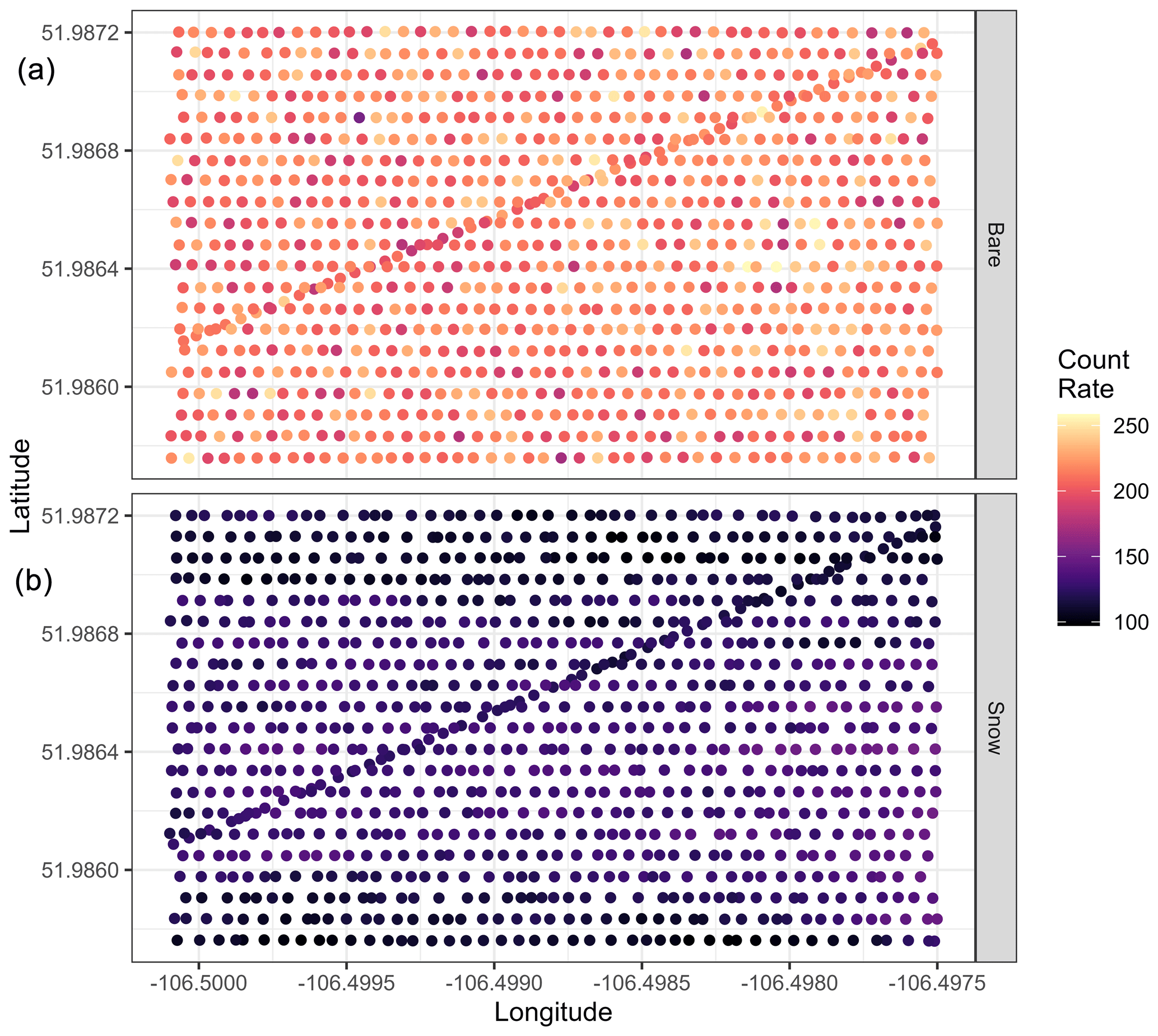
Figure A1Raw count rates (colour) and positioning for the grassland study site before snow accumulation (a) and at peak accumulation (b).
Balancing SWE observation resolution and UAV platform limitations is the main challenge to employing UAV-based gamma methods to quantify the spatial variability of SWE. Variations in flight line spacing, altitude, and velocity influence the scale of resolvable features and flight planning best practices to inform future operations can be gleaned from this experience. Generally, two thirds of gamma counts originate from a footprint area twice the altitude in width and twice the altitude in addition to the distance travelled in length (Ward, 1981). Based on flight profiles, this means the approximate footprints for stubble profiles are 1050 m2 (30 m resolution) and for grassland profiles are 320 m2 (16 m resolution). The relationship between flight altitude, line spacing, and velocity and resolution associated with a 20 s integration time is simulated applying the (Ward, 1981) footprint approximation in a drop-in-the-bucket (DIB) approach (Fig. B1). The simulated resolutions range from 4.5 m with a flight profile with a 1 m s−1 velocity, 1 m altitude, and 1 m altitude to a 65 m resolution with a flight profile with a 10 m s−1 velocity, altitude of 15 m, and line spacing of 15 m. The stubble flight profile aligns with a 53 m footprint resolution, which demonstrates the challenges the error versus resolution patterns demonstrated in Sec 4.3 which had high errors up to the maximum 50 m resolution tested. In contrast, the grassland profile aligns with a 30 m footprint resolution which aligns with the plateauing of errors in the 20–30 m resolution range (Fig. 4). The relative implications of flight profiles for resolvable features can be estimated from the interaction visualized in Fig. B1. In uniform landscape classes on the Canadian Prairies, sampling needs to span length scales between 30 and 100 m to capture the spatial variability of SWE (Shook and Gray, 1996); it is apparent that the grassland flight profile employed is on the edge of capturing SWE variability appropriately. Further tests of lower, slower and closer flight lines are needed. At altitudes approaching 1 m hardware, demands increase as real-time terrain-following guidance systems and RTK precision are needed for navigation and position logging. The system employed in this study did not have these features, and so these profiles could not be tested. The influence of atmospheric attenuation will vary with altitude and is not considered in this conceptual flight profile versus resolution simulation.
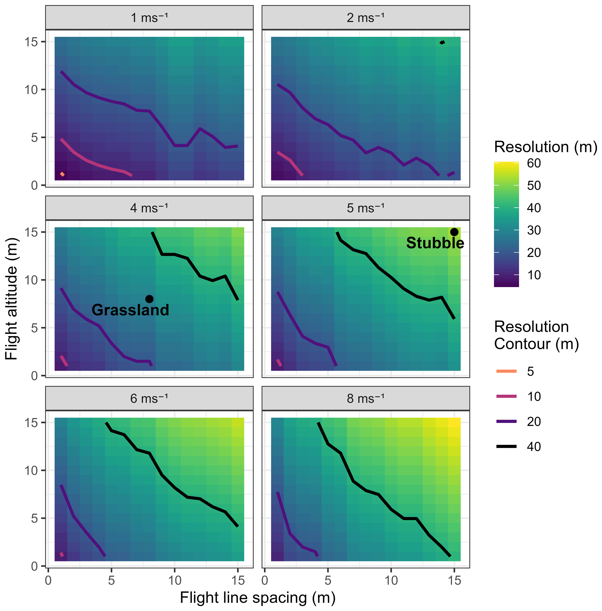
Figure B1Relationship between flight altitude (vertical axis), line spacing (horizontal axis), and platform velocity (panels) versus estimated resolution (fill colour) for a 20 s integration time. Contour lines of 5, 10, 20, and 40 m resolutions and the points corresponding to the stubble and grassland flight profiles are plotted.
The underlying datasets (snow survey observations, lidar snow depth maps, gamma count rates, and snow water equivalent maps (reference (from lidar and observed snow density), gamma, and lidar–gamma fusion) are available through the Federated Research Data Repository (https://doi.org/10.20383/103.0846, Harder et al., 2023).
PH, WDH, and JWP defined the research objectives; PH and WDH performed the fieldwork; and PH completed the data analysis and interpretation and manuscript preparation. All authors contributed to discussions and revisions of the manuscript.
The contact author has declared that none of the authors has any competing interests.
Publisher's note: Copernicus Publications remains neutral with regard to jurisdictional claims made in the text, published maps, institutional affiliations, or any other geographical representation in this paper. While Copernicus Publications makes every effort to include appropriate place names, the final responsibility lies with the authors.
Funding for this work comes from the Canada First Research Excellence Fund through the Global Water Futures programme, Canadian Foundation for Innovation, Western Economic Diversification, and the Canada Research Chairs programme. Field and technical assistance from Bruce Johnson, Anders Hunter, Alistair Wallace, and Medusa Radiometrics is gratefully acknowledged.
This research has been supported by the Canada First Research Excellence Fund (grant no. CFREF-2015-00010), the Natural Sciences and Engineering Research Council of Canada (grant no. CRC-2016-00144), the Western Economic Diversification Canada (grant no. 000014400), and the Canada Foundation for Innovation (grant no. 37227).
This paper was edited by Edward Bair and reviewed by Eunsang Cho and Christopher Donahue.
Bühler, Y., Adams, M. S., Bösch, R., and Stoffel, A.: Mapping snow depth in alpine terrain with unmanned aerial systems (UASs): potential and limitations, The Cryosphere, 10, 1075–1088, https://doi.org/10.5194/tc-10-1075-2016, 2016.
Carroll, S. S. and Carroll, T. R.: Effect of uneven snow cover on airborne snow water equivalent estimates obtained by measuring terrestrial gamma radiation, Water Resour. Res., 25, 1505–1510, https://doi.org/10.1029/WR025i007p01505, 1989.
Carroll, T.: Airborne Gamma Radiation Snow Survey Program: A User's Guide, Version 5. 0, National Operation Hydrologic Remote Sensing Center, Chanhassen, Minnesota, 14 pp., https://www.nohrsc.noaa.gov/technology/pdf/tom_gamma50.pdf (last access: 16 July 2024), 2001.
Cho, E., Jacobs, J. M., and Vuyovich, C. M.: The Value of Long-Term (40 years) Airborne Gamma Radiation SWE Record for Evaluating Three Observation-Based Gridded SWE Data Sets by Seasonal Snow and Land Cover Classifications, Water Resour. Res., 56, 23, https://doi.org/10.1029/2019WR025813, 2019.
Cho, E., Jacobs, J. M., Schroeder, R., Tuttle, S. E., and Olheiser, C.: Improvement of operational airborne gamma radiation snow water equivalent estimates using SMAP soil moisture, Remote Sens. Environ., 240, 111668, https://doi.org/10.1016/j.rse.2020.111668, 2020.
Coles, G. A., Graham, D. R., and Allision, R. D.: Experience Gained Operating Snow Pillows on a near Real-Time Basis on the Mountainous Areas of Alberta, in: Workshop on Snow Property Measurement, Lake Louise, Alberta, 13, https://research-groups.usask.ca/hydrology/documents/pubs/papers/coles_et_al_1985.pdf (last access: 16 July 2024), 1985.
DeBeer, C. M. and Pomeroy, J. W.: Simulation of the snowmelt runoff contributing area in a small alpine basin, Hydrol. Earth Syst. Sci., 14, 1205–1219, https://doi.org/10.5194/hess-14-1205-2010, 2010.
Deems, J., Painter, T., and Finnegan, D.: Lidar measurement of snow depth: a review, J. Glaciol., 59, 467–479, https://doi.org/10.3189/2013JoG12J154, 2013.
Essery, R. and Pomeroy, J.: Implications of spatial distributions of snow mass and melt rate for snow-cover depletion: theoretical considerations, Ann. Glaciol., 38, 261–265, https://doi.org/10.3189/172756404781815275, 2004a.
Essery, R. and Pomeroy, J.: Vegetation and Topographic Control of Wind-Blown Snow Distributions in Distributed and Aggregated Simulations for an Arctic Tundra Basin, J. Hydrometeorol., 5, 735–744, https://doi.org/10.1175/1525-7541(2004)005<0735:VATCOW>2.0.CO;2, 2004b.
Faria, D. A., Pomeroy, J. W., and Essery, R. L. H.: Effect of covariance between ablation and snow water equivalent on depletion of snow-covered area in a forest, Hydrol. Process., 14, 2683–2695, https://doi.org/10.1002/1099-1085(20001030)14:15<2683::AID-HYP86>3.0.CO;2-N, 2000.
Fernández, A.: An energy balance model of seasonal snow evolution, Phys. Chem. Earth, 23, 661–666, https://doi.org/10.1016/S0079-1946(98)00107-4, 1998.
Filhol, S. and Sturm, M.: Snow bedforms: A review, new data, and a formation model, J. Geophys. Res.-Earth, 120, 1645–1669, https://doi.org/10.1002/2015JF003529, 2015.
Gray, D. M. and Landine, P. G.: An Energy-Budget Snowmelt Model for the Canadian Prairies, Can. J. Earth Sci., 25, 1292–1303, 1988.
Grünewald, T., Schirmer, M., Mott, R., and Lehning, M.: Spatial and temporal variability of snow depth and ablation rates in a small mountain catchment, The Cryosphere, 4, 215–225, https://doi.org/10.5194/tc-4-215-2010, 2010.
Harder, P., Schirmer, M., Pomeroy, J., and Helgason, W.: Accuracy of snow depth estimation in mountain and prairie environments by an unmanned aerial vehicle, The Cryosphere, 10, 2559–2571, https://doi.org/10.5194/tc-10-2559-2016, 2016.
Harder, P., Pomeroy, J. W., and Helgason, W. D.: Implications of stubble management on snow hydrology and meltwater partitioning, Can. Water Resour. J./Rev. Can. des ressources hydriques, 44, 193–204, https://doi.org/10.1080/07011784.2019.1575774, 2019.
Harder, P., Pomeroy, J. W., and Helgason, W. D.: Improving sub-canopy snow depth mapping with unmanned aerial vehicles: lidar versus structure-from-motion techniques, The Cryosphere, 14, 1919–1935, https://doi.org/10.5194/tc-14-1919-2020, 2020.
Harder, P., Helgason, W., and Pomeroy, J.: UAV-borne gamma spectrometry and lidar observations of prairie snow water equivalent, Federated Research Data Repository [data set], https://doi.org/10.20383/103.0846, 2023.
He, Z., Shook, K., Spence, C., Pomeroy, J. W., and Whitfield, C. J.: Modeling the sensitivity of snowmelt , soil moisture and streamflow generation to climate over the Canadian Prairies using a basin classification approach, Hydrol. Earth Syst. Sci., 2023.
Hendriks, P. H. G. M., Limburg, J., and de Meijer, R. J.: Full-spectrum analysis of natural gamma-ray spectra, J. Environ. Radioact., 53, 365–380, 2001.
Hopkinson, C. and Collins, T.: Alberta front ranges lidar snow depth assessment: Final report, Applied Geomatics Research Group, Middleton, NS, 55 pp., 2009.
Isenburg, M.: LAStools – Efficient LiDAR Processing Software, rapidlasso GmbH [software], http://rapidlasso.com/LAStools (last access: 7 July 2024), 2019.
Jacobs, J. M., Hunsaker, A. G., Sullivan, F. B., Palace, M., Burakowski, E. A., Herrick, C., and Cho, E.: Snow depth mapping with unpiloted aerial system lidar observations: a case study in Durham, New Hampshire, United States, The Cryosphere, 15, 1485–1500, https://doi.org/10.5194/tc-15-1485-2021, 2021.
Janowicz, J. R., D. M. Gray, and J. W. Pomeroy: Spatial variability of fall soil moisture and spring snow water equivalent within a mountainous sub-arctic watershed, in: Proceedings of the Eastern Snow Conference, vol. 60, 127–139, https://research-groups.usask.ca/hydrology/documents/pubs/papers/janowicz_et_al_2003.pdf (last access: 16 July 2024), 2003.
Kinar, N. J. and Pomeroy, J. W.: Determining snow water equivalent by acoustic sounding, Hydrol. Process., 21, 2623–2640, 2007.
Kinar, N. J. and Pomeroy, J. W.: Measurement of the physical properties of the snowpack, Rev. Geophys., 53, 481–544, https://doi.org/10.1002/2015RG000481, 2015.
King, J., Pomeroy, J. W., Gray, D. M., Fierz, C., Fohn, P. M. B., Harding, R. J., Jordan, R., Martin, E., and Pluss, C.: Snow – atmosphere energy and mass balance, in: Snow and Climate: Physical Processes, Surface Energy Exchange and Modeling, edited by: Armstrong, R. and Brun, E., Cambridge University Press, Cambridge, England, 70–124, ISBN 9780521854542, 2008.
Liston, G. E. and Sturm, M.: A snow-transport model for complex terrain, J. Glaciol., 44, 498–516, https://doi.org/10.3189/S0022143000002021, 1998.
Long, D. G., Brodzik, M. J., and Hardman, M. A.: Enhanced-Resolution SMAP Brightness Temperature Image Products, IEEE T. Geosci. Remote, 57, 4151–4163, https://doi.org/10.1109/TGRS.2018.2889427, 2019.
Marti, R., Gascoin, S., Berthier, E., de Pinel, M., Houet, T., and Laffly, D.: Mapping snow depth in open alpine terrain from stereo satellite imagery, The Cryosphere, 10, 1361–1380, https://doi.org/10.5194/tc-10-1361-2016, 2016.
Martin, P. G., Connor, D. T., Estrada, N., El-turke, A., Megson-smith, D., Jones, C. P., Kreamer, D. K., and Scott, T. B.: Radiological identification of near-surface mineralogical deposits using low-altitude unmanned aerial vehicle, Remote Sens.-Basel, 12, 1–16, https://doi.org/10.3390/rs12213562, 2020.
Medusa Radiometrics: Gamman Manual, Medusa Radiometrics BV, https://docs.medusa-radiometrics.com/gamman-manual/latest/software-reference (last access: 11 April 2024).
Offenbacher, E. L. and Colbeck, S. C.: Remote Sensing of Snow Covers Using the Gamma-Ray Technique, CRREL Report 91-9, Cold Regions Research & Engineering Laboratory, Hanover, New Hampshire, 25 pp., http://hdl.handle.net/11681/9113 (last access: 16 July 2024), 1991.
Painter, T. H., Berisford, D. F., Boardman, J. W., Bormann, K. J., Deems, J. S., Gehrke, F., Hedrick, A., Joyce, M., Laidlaw, R., Marks, D., Mattmann, C., McGurk, B., Ramirez, P., Richardson, M., Skiles, S. M. K., Seidel, F. C., and Winstral, A.: The Airborne Snow Observatory: Fusion of scanning lidar, imaging spectrometer, and physically-based modeling for mapping snow water equivalent and snow albedo, Remote Sens. Environ., 184, 139–152, https://doi.org/10.1016/j.rse.2016.06.018, 2016.
Peck, E. L., Bissell, V. C., Jones, E. B., and Burge, D. L.: Evaluation Snow Water Equivalent by Airborne Measurement of Passive Terrestrial Gamma Radiation, Water Resour. Res., 17, 1425–1430, https://doi.org/10.1029/WR007i005p01151, 1971.
Pomeroy, J. W. and Goodison, B. E.: Winter and Snow, in: The Surface Climates of Canada, edited by: Bailey, W. G., Oke, R., and Rouse, W. R., McGill-Queen's Univ Press, Montreal, ISBN 0-7735-1672-7, 68–100, 1997.
Pomeroy, J. W. and Gray, D. M.: Snow accumulation, relocation and management, Science Report No. 7, National Hydrology Research Institute, Environment Canada, Saskatoon, SK, 144 pp., 1995.
Pomeroy, J. W., Gray, D. M., Shook, K. R., Toth, B., Essery, R. L. H., Pietroniro, A., and Hedstrom, N.: An evaluation of snow accumulation and ablation processes for land surface modelling, Hydrol. Process., 12, 2339–2367, https://doi.org/10.1002/(SICI)1099-1085(199812)12:15<2339::AID-HYP800>3.0.CO;2-L, 1998.
Pomeroy, J. W., de Boer, D., and Martz, L. W.: Hydrology and Water Resources, in: Saskatchewan Geographic Perspectives, edited by: Thraves, B. D., Lewry, M. L., Dale, J. E., and Schlichtmann, H., Canadian Plains Research Center, University of Regina, Regina Saskatchewan 63–80, ISBN 978 0 88977 189 5, 2007.
Reinhardt, N. and Herrmann, L.: Gamma-ray spectrometry as versatile tool in soil science: A critical review, J. Plant Nutr. Soil Sc., 182, 9–27, https://doi.org/10.1002/jpln.201700447, 2019.
Shook, K. and Gray, D. M.: Small-Scale Spatial Structure of Shallow Snowcovers, Hydrol. Process., 10, 1283–1292, 1996.
Shook, K., Gray, D. M., and Pomeroy, J. W.: Temporal Variation in Snowcover Area During Melt in Prairie and Alpine Environments, Nord. Hydrol., 24, 183–198, 1993.
Smith, C. D., Kontu, A., Laffin, R., and Pomeroy, J. W.: An assessment of two automated snow water equivalent instruments during the WMO Solid Precipitation Intercomparison Experiment, The Cryosphere, 11, 101–116, https://doi.org/10.5194/tc-11-101-2017, 2017.
Steppuhn, H.: Accuracy in Estimating Snow Cover Water Equivalents, in: Canadian Hydrology Symposium, in: Canadian Hydrology Symposium – 1975 Proceedings, 11–14 August 1975, Winnipeg, Manitoba, Associate Committee on Hydrology, National Research Council of Canada, 5, https://research-groups.usask.ca/hydrology/documents/pubs/papers/steppuhn_1975.pdf (last access: 16 July 2024), 1975.
Steppuhn, H. and Dyck, G. E.: Estimating True Basin Snowcover, in: Proceedings of Interdisciplinary Symposium on Advanced Concepts and Techniques in the Study of Snow and Ice Resourses, Washington, DC, The National Academies Press, 314–328, https://research-groups.usask.ca/hydrology/documents/pubs/papers/steppuhn_dyck_1974.pdf (last access: 16 July 2024), 1974.
Tedesco, M., Derksen, C., Deems, J. S., and Foster, J. L.: Remote sensing of snow depth and snow water equivalent, in: Remote Sensing ofthe Cryosphere, edited by: Tedesco, M., John Wiley & Sons, Ltd, 73–98, ISBN 9781118368855, 2015.
Tong, J., Déry, S. J., Jackson, P. L., and Derksen, C.: Testing snow water equivalent retrieval algorithms for passive microwave remote sensing in an alpine watershed of western Canada, Can. J. Remote Sens., 36, S74–S86, https://doi.org/10.5589/m10-009, 2010.
Topp, G. C.: Soil Water Content from Gamma Ray Attenuation: A Comparision of Ionization Chamber and Scintillation Detectors, Can. J. Soil Sci., 50, 439–447, 1970.
Trujillo, E., Ramý, J. A., and Elder, K.: Topographic, meteorologic, and canopy controls on the scaling characteristics of the spatial distribution of snow depth fields, Water Resour. Res., 43, W07409, https://doi.org/10.1029/2006WR005317, 2007.
Tsang, L., Durand, M., Derksen, C., Barros, A. P., Kang, D.-H., Lievens, H., Marshall, H.-P., Zhu, J., Johnson, J., King, J., Lemmetyinen, J., Sandells, M., Rutter, N., Siqueira, P., Nolin, A., Osmanoglu, B., Vuyovich, C., Kim, E., Taylor, D., Merkouriadi, I., Brucker, L., Navari, M., Dumont, M., Kelly, R., Kim, R. S., Liao, T.-H., Borah, F., and Xu, X.: Review article: Global monitoring of snow water equivalent using high-frequency radar remote sensing, The Cryosphere, 16, 3531–3573, https://doi.org/10.5194/tc-16-3531-2022, 2022.
Tuttle, S. E., Jacobs, J. M., Vuyovich, C. M., Olheiser, C., and Cho, E.: Intercomparison of snow water equivalent observations in the Northern Great Plains, Hydrol. Process., 32, 817–829, https://doi.org/10.1002/hyp.11459, 2018.
Walker, B., Wilcox, E. J., and Marsh, P.: Accuracy assessment of late winter snow depth mapping for tundra environments using structure-from-motion photogrammetry, Arctic Science, 7, 588–604, https://doi.org/10.1139/as-2020-0006, 2021.
Ward, S. H.: Gamma-Ray Spectrometry in Geologic Mapping and Uranium Exploration, Econ. Geol., https://doi.org/10.5382/AV75.24, 1981.
Wright, M., Kavanaugh, J., and Labine, C.: Performance Analysis of GMON3 Snow Water Equivalency Sensor, in: Western Snow Conference, Stateline, Nevada 18–21 April 2011, 105–108, https://westernsnowconference.org/bibliography/2011Wright.pdf (last access: 16 July 2024), 2011.
- Abstract
- Introduction
- Data and methods
- Results
- Discussion
- Conclusions
- Appendix A: Raw count rates
- Appendix B: Flight planning best practices for UAV-based gamma SWE observations
- Data availability
- Author contributions
- Competing interests
- Disclaimer
- Acknowledgements
- Financial support
- Review statement
- References