the Creative Commons Attribution 4.0 License.
the Creative Commons Attribution 4.0 License.
 | 04 Jul 2024
Seasonal and diurnal variability of sub-ice platelet layer thickness in McMurdo Sound from electromagnetic induction sounding
Gemma M. Brett
Greg H. Leonard
Wolfgang Rack
Christian Haas
Patricia J. Langhorne
Natalie J. Robinson
Anne Irvin
Here, we present observations of temporal variability of sub-ice platelet layer over seasonal and diurnal timescales under Ice Shelf Water-influenced fast ice in McMurdo Sound. Electromagnetic induction (EM) sounding time-series measurements of the thicknesses of fast ice and sub-ice platelet layer were made in winter and late spring of 2018. Winter objectives were to measure the seasonal growth of fast ice and sub-ice platelet layer near the McMurdo Ice Shelf in the east, while in late spring we assessed the diurnal variability of sub-ice platelet layer with coincident EM time-series and oceanographic measurements collected in the main outflow path of supercooled Ice Shelf Water in the west. During winter, we observed when the sub-ice platelet layer formed beneath consolidated ice. Episodes of rapid sub-ice platelet layer growth (∼ 0.5–1 m) coincided with strong southerly wind events and polynya activity, suggesting wind-enhanced Ice Shelf Water circulation from the McMurdo–Ross Ice Shelf cavity. In late spring, we investigated how the tides and ocean properties influenced the sub-ice platelet layer. Over a 2-week neap–spring tidal cycle, changes in sub-ice platelet layer thickness were observed to correlate with the tides, increasing more during neap than spring tide cycles, and on diurnal timescales, more on ebb than flood tides. Neap and ebb tides correspond with stronger northward circulation out of the cavity, indicating that sub-ice platelet layer growth was driven by tidally enhanced Ice Shelf Water outflow. The observed variability indicated that wind-driven circulation and the tides influence Ice Shelf Water outflow in McMurdo Sound and, consequently, sub-ice platelet layer evolution over a range of timescales.
- Article
(9501 KB) - Full-text XML
- BibTeX
- EndNote


In the western Ross Sea, sea ice production in coastal polynyas forms High Salinity Shelf Water (HSSW) (Ohshima et al., 2016), which circulates into the conjoined McMurdo–Ross Ice Shelf cavity (Fig. 1) and drives basal melting at depth in the grounding zone (Jacobs et al., 1992). The resultant meltwater has a potential temperature below the surface freezing point (Jacobs et al., 1985) and is classified as Ice Shelf Water (ISW). The buoyant rise of relatively fresh ISW from deep source regions in the cavity (MacAyeal, 1984), and consequent pressure decrease, induces in situ supercooling (Foldvik and Kvinge, 1974; Jenkins and Bombosch, 1995) and frazil ice formation (Holland and Feltham, 2005; Robinson et al., 2014). Frazil ice grows into larger platelet ice crystals with continued immersion in supercooled ISW (Smith et al., 2012).
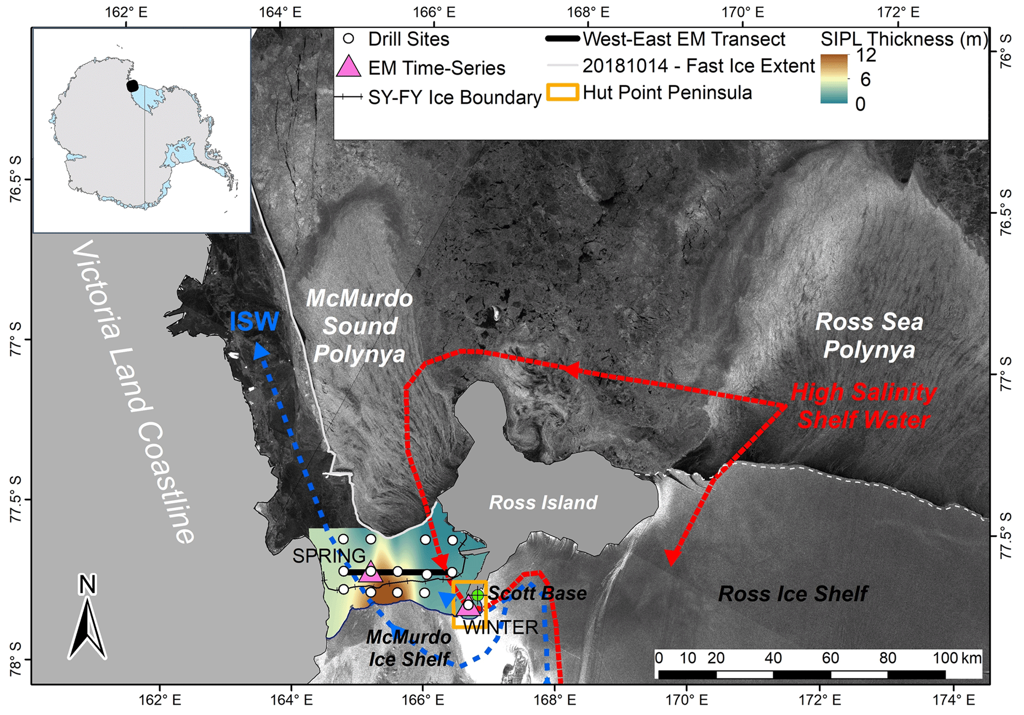
Figure 1McMurdo Sound, western Ross Sea, Antarctica (inset map), with dashed lines illustrating HSSW (red), formed within the Ross Sea and McMurdo Sound polynyas, circulating into the conjoined McMurdo–Ross Ice Shelf cavity and ISW (blue) outflow into McMurdo Sound. The late-spring fast-ice edge (grey line) and boundary between second-year (SY) and first-year (FY) fast ice present in the study region in 2018 are shown with the locations of the Winter and Spring EM time-series sites (pink triangles) and the electronic weather station (EWS) at Scott Base (green crossed circle). SIPL thickness distribution was spline interpolated from drill hole measurements made at 14 drill sites (white circles) in November 2018, along with repeated west–east EM transects (black line) across McMurdo Sound. At the Spring site, we additionally carried out repeated 200 m × 200 m grid surveys and collected oceanographic data at a mooring deployed (500 m to the north) in November 2018 (satellite image: Sentinel-1 SAR, 2 October 2018).
In McMurdo Sound, supercooled ISW with a suspension of frazil and platelet ice crystals reaches the upper surface ocean (Hughes et al., 2014; Lewis and Perkin, 1985; Robinson et al., 2014). Ice crystals are deposited beneath fast ice in proximity to the McMurdo Ice Shelf where they can continue to grow in situ (Leonard et al., 2011; Smith et al., 2001). Through congelation growth of sea ice, platelet ice crystals freeze into the sea ice base forming incorporated platelet ice (Smith et al., 2012, 2001). Once the freezing rate of the sea ice becomes sufficiently low (Wongpan et al., 2021) and is exceeded by the rate of ice crystal deposition from the water column (Dempsey et al., 2010; Gough et al., 2012; Hoppmann et al., 2015a), an unconsolidated mass of platelet ice crystals called a sub-ice platelet layer (SIPL) can form. The abundance of platelet ice provides a quantifiable metric of ice mass transfer (Lewis and Perkin, 1986) from deep glacial source regions to the ocean surface. Indeed, the thickness distribution and volume of consolidated platelet ice and SIPL in McMurdo Sound are the manifestation of supercooled ISW outflow (Langhorne et al., 2015) and thus the regional atmospheric and oceanographic processes driving polynya activity and HSSW and ISW formation in the western Ross Sea (Brett et al., 2020).
The development of a supercooled ISW plume over winter in McMurdo Sound and its effects on fast ice formation have been investigated in previous studies (Gough et al., 2012; Hunt et al., 2003; Leonard et al., 2011, 2006; Mahoney et al., 2011). The annual spatial distributions of ISW-influenced fast ice and SIPL have been observed over multiple years in McMurdo Sound using a variety of techniques including ice coring (Dempsey et al., 2010; Gough et al., 2012), drill hole measurements (Langhorne et al., 2015), electromagnetic induction (EM) sounding (Brett et al., 2020; Haas et al., 2021; Rack et al., 2013), and satellite altimetry (Brett et al., 2021; Price et al., 2015, 2013). However, most observations were collected in late spring, towards the end of the sea ice growth season, and captured a snapshot of a fully developed fast ice cover and SIPL.
Given the difficulty of carrying out in situ measurements (especially in winter), the growth of SIPL has never been continuously assessed in high temporal resolution (Hoppmann et al., 2020). SIPL evolution over winter has not been frequently observed nor has variability in its thickness over short diurnal timescales (Hoppmann et al., 2020). In Atka Bay, Queen Maud Land, SIPL and fast ice growth during winter were observed by drill hole measurements made every 2–5 weeks (Arndt et al., 2020; Hoppmann et al., 2015a, b). Similar low temporal resolution drill hole surveys have been made in McMurdo Sound throughout winter (Leonard et al., 2006; Purdie et al., 2006; Mahoney et al., 2011; Gough et al., 2012). However, neither diurnal variability in SIPL nor inferences on short timescale processes were resolved. In McMurdo Sound, EM techniques were applied to obtain high-resolution spatial measurements of fast ice and SIPL thickness in late spring over multiple years (Brett et al., 2020; Haas et al., 2021). In repeat EM surveys near Hut Point Peninsula (refer to Fig. 1 for location) in eastern McMurdo Sound, Brett et al. (2020) detected significant increases in SIPL thickness (∼ 1 m) occurring over short timescales of days, indicating that an additional forcing more episodic than gradual platelet ice accretion is driving SIPL evolution on short diurnal timescales. Camera observations of individual platelet ice crystals at the base of the SIPL in eastern McMurdo Sound in 2000 (Smith et al., 2012) and 2003 (Leonard et al., 2006) revealed episodic growth bursts of 1–12 cm d−1 during neap tides.
In McMurdo Sound, temporal variability in SIPL thickness distribution is considered to be strongly coupled to variability in the distribution and volume of supercooled ISW circulating out from the ice shelf cavity and beneath the fast ice (Langhorne et al., 2015). ISW outflow, in turn, should be influenced by seasonal changes in regional ocean circulation and on shorter timescales by the tides and episodic forcing such as strong wind events and polynya activity. In this study, we used EM time-series measurements carried out in winter of 2018 to assess the growth of ISW-influenced fast ice and the SIPL near the McMurdo Ice Shelf in the east and in the following late spring over a neap–spring tidal cycle in the main path of ISW outflow in the west (Fig. 1). From the winter EM time series, we identified when the SIPL started to form and captured how it evolved seasonally and in response to strong wind events and satellite-observed polynya activity. In late spring, we used coincident EM time-series and oceanographic measurements to investigate how the tides and ocean properties influenced SIPL over a 2-week neap–spring tidal cycle. We describe the study area and methods in Sect. 2, the results in Sect. 3, and in Sect. 4 we consider our observations in relation to oceanography, episodic wind-driven polynya activity, and the tides in McMurdo Sound.
Figure 1 shows the McMurdo Sound study region located in the western Ross Sea. McMurdo Sound has distinct oceanographic regimes from east to west as illustrated in Fig. 1. In the east, the deep Erebus Basin (700 m) provides a conduit for water mass exchange between open ocean in the Ross Sea and the conjoined McMurdo–Ross Ice Shelf cavity (Assmann et al., 2003; Hunt et al., 2003; Leonard et al., 2011, 2006; Mahoney et al., 2011; Robinson et al., 2010; Stern et al., 2013). Near-surface current directions are variable in the east but predominantly flow south and into the cavity throughout summer in the Hut Point Peninsula region (Barry and Dayton, 1988; Barry, 1988; Hunt et al., 2003; Leonard et al., 2011, 2006; Mahoney et al., 2011; Robinson et al., 2010; Stern et al., 2013). In autumn (March and April), surface currents in eastern McMurdo Sound switch to a northerly direction and out from the ice shelf cavity (Leonard et al., 2011, 2006; Mahoney et al., 2011). In the west, the bathymetry is shallower (200–300 m), and the dominant near-surface flow regime is out from the cavity, to the north, and consists of supercooled ISW with a frazil ice suspension (Barry, 1988; Lewis and Perkin, 1985; Robinson et al., 2014).
The regional oceanography results in a consistent late-spring pattern of thicker fast ice and SIPL in western McMurdo Sound (Brett et al., 2020), which was also observed in November 2018 in drill hole spatial surveys (Brett et al., 2023) (Fig. 1). The fast ice consisted of a 7–15 km wide band of second-year ice that ran parallel to the McMurdo Ice Shelf in the south and more typical first-year ice in the north. The spatial distribution of SIPL thickness was characteristic of McMurdo Sound, with very thick accumulations in the main region of ISW outflow in the centre and west as shown in Fig. 1.
On shorter timescales, we expect that episodic forcings such as strong wind events and polynya activity will influence ocean circulation in McMurdo Sound on timescales of days. In winter 2003 in the eastern sound, Leonard et al. (2006) observed pulses of supercooled ISW outflow associated with increased acoustic backscatter indicative of suspended ice crystals in the upper water column. These pulses could not always be attributed to tidal forcing. To investigate this phenomenon, we assessed temporal variability of SIPL thickness observed in winter in relation to wind data obtained at an electronic weather station (EWS) at Scott Base (Fig. 1) and polynya activity observed in Sentinel-1 SAR and NASA Worldview MODIS satellite images.
On diurnal timescales, the 13.66 d spring–neap cycle (Goring and Pyne, 2003) and diurnal tides in McMurdo Sound influence ocean circulation. In eastern McMurdo Sound, peak southward and northward flows were observed on flood and ebb spring tides, respectively (Leonard et al., 2006; Robinson et al., 2010). In western McMurdo Sound, currents generally persist to the north-northwest, flowing out of the ice shelf cavity on flood and ebb tides (Jendersie et al., 2018; Robinson et al., 2014) except on incursions of spring flood tides when weaker reversal of flows to the southeast have been observed (Frazer et al., 2020). Arrigo et al. (1995) observed that nutrient exchange within the SIPL in McMurdo Sound co-varied with the tides, which they postulated was caused by tidally induced seawater exchange at the SIPL–ocean interface. To investigate tidal influence on the SIPL, we evaluated how SIPL thickness changed over neap and spring tidal cycles and flood and ebb tidal ranges in EM time-series measurements made in late spring as described in Sect. 2.1.
2.1 EM time-series measurements
Electromagnetic induction (EM) sounding time-series measurements of fast ice and SIPL growth in McMurdo Sound were made during winter (8 August to 27 October 2018) in the east and in the following late spring (4–18 November 2018) in the west (refer to Fig. 1) with a single-frequency (9.8 kHz, 3.66 m coil spacing) Geonics Ltd EM31-MK2 instrument. For all EM measurements in this study, the EM31 was configured in vertical-dipole mode with a conductivity sensitivity range of 1000 mS m−1. In winter and spring, different deployment set-ups for the EM31 were used, and separate drill hole campaigns were carried out for EM data processing (Sect. 2.2), which are described in detail in their respective sections below.
For both EM time-series deployments, power was supplied by a 12 V battery and data were recorded at 10 min (winter) or 5 min (spring) intervals by a Campbell Scientific CR3000 data logger, which also logged ambient air temperature. At each sampling interval in both winter and spring, the EM31 was programmed to power up for 60 s before acquiring data at 1 Hz for another 60 s. The standard deviation of the 60 measurements made every 5 or 10 min was used to identify low-quality in-phase and quadrature data converted to parts per million (ppm) (i.e. ratio of the secondary EM field to the primary EM field generated by the EM31). Values exceeding the mean standard deviations were flagged as low quality and removed.
In winter, EM31 measurements were subject to a strong temperature drift in response to very low and highly variable temperatures (−48 to −4 °C). By comparing the variability of EM measurements with coincident air temperatures, we developed an algorithm for temperature correction of the EM data, which is described in the Appendix. All results presented for the winter EM time series in the main text are for temperature-corrected EM data. In spring, given higher and less variable air temperatures (−12 to +7 °C), and our ability to regularly change the EM31 batteries, temperature drift was not significant (refer to the Appendix).
In winter, the mean standard deviations for in-phase and quadrature data were ∼ 17 and ∼ 200 ppm, respectively. Generally, the standard deviations exceeded these values substantially (by a factor of 100) when the air temperature was below −30 °C (in winter) and were easily identified for omission. All EM data in the spring time series were determined to be of high quality from standard deviations, which never exceeded mean values of ∼ 20 ppm for in-phase and ∼ 100 ppm for quadrature data. The difference in standard deviations is driven by the quadrature being twice as large in magnitude as the in-phase data and considerably more variable. Additionally, in-phase data measured by the EM31 require calibration (gain and offset) to be applied as described in Sect. 2.2.
2.1.1 Winter EM time series
In the east, EM time-series measurements were made in winter of 2018 at a site (166.655° E, 77.867° S) in the Hut Point Peninsula region (i.e. where Brett et al. (2020) observed diurnal variability in SIPL thickness), ∼ 5 km north of the McMurdo Ice Shelf. We refer to this as the Winter time series (Fig. 1), and its aim was to observe the growth of fast ice and SIPL. The EM31 was integrated into the University of Otago's Sea Ice Monitoring Station (SIMS) with a thermistor probe and a snow sensor (Richter et al., 2023). The EM31 was deployed in a weather-proof wooden box on the sea ice surface (snow layer removed) of second-year fast ice from 8 August to 27 October 2018. The near-real-time winter fast ice, and SIPL measurements were radio-telemetered to Scott Base (Fig. 1) and then forwarded to the University of Otago in New Zealand. The Winter EM observations were carried out for 80 d (1920 h) with 1342 h of high-quality data collected (Brett et al., 2024a). The instrument generally operated well, except when the battery voltage fell below 11 V or when ambient air temperature measured by the data logger was below −30 °C for prolonged periods of time. Drill hole measurements of fast ice and SIPL thicknesses at the Winter site were made every 3–4 weeks (4 in total) by Scott Base winter staff. An additional drill hole measurement was made on 19 November 2018 by the authors, 23 d after the survey ended. Due to logistical constraints, no oceanographic data were collected with the Winter EM time-series measurements.
2.1.2 Spring EM time series
In the following late spring (November 2018), EM time-series measurements were carried out during a neap–spring tidal cycle in the main path of ISW outflow, ∼ 12 km north of the McMurdo Ice Shelf, in western McMurdo Sound, which we refer to as the Spring site (Fig. 1). We additionally observed temporal changes at two larger spatial scales with respect to the neap–spring tidal cycle: repeated 200 m × 200 m grid surveys (50 m line spacing) carried out near the Spring site and repeated EM surveys on a ∼ 50 km west–east transect across the sound (latitude 77.767° S) (Fig. 1; Brett et al., 2024b). For the Spring EM time series, the EM31 was deployed on a sledge (snow layer not removed) at a drill hole site (165.2° E, 77.767° S) on the long west–east transect (refer to Figs. 1 and 7b for location) when it was not being used for spatial EM surveys. A total of 202 h of EM time-series data were collected between 4 and 18 November 2018 over five separate time intervals ranging from 12–70 h (Brett et al., 2024c). The Spring EM time series was collected with coincident oceanographic measurements of temperature and salinity (Fig. 1) from a mooring deployed 500 m to the north, which is described in Sect. 2.4. In spring, 44 drill hole measurements of fast ice and SIPL thickness collected at 9 drill sites (i.e. ∼ 5 at each of the drill sites) on first-year fast ice only (i.e. north of second-year fast ice boundary in Fig. 1) were used to calibrate (Sect. 2.2) all late-spring EM measurements including the Spring time series, repeat west–east transects, and grid surveys. Over each drill hole, geo-located EM measurements were made with the EM31 for a continuous period of 20 s.
2.2 Forward modelling and inversion of EM measurements
The EM processing method (Irvin, 2018) demonstrated by Brett et al. (2020) was applied in this study to simultaneously obtain sea ice and SIPL thicknesses from single-frequency EM in-phase (I) and quadrature (Q) measurements by inversion of forward modelled EM responses over different conductive horizonal layers: (1) consolidated ice (including the generally thin snow layer), (2) a SIPL, and (3) infinitely deep seawater. We assumed the following conductivities: 0 mS m−1 for consolidated ice and snow (Haas, 1997), 2700 mS m−1 for seawater, typical for McMurdo Sound (Mahoney et al., 2011) and observed in this study (Fig. 5c), and a range of bulk conductivity values for the SIPL (100–1500 mS m−1; Haas et al., 2021). The conductivity of first-year sea ice has a typical range of 0–50 mS m−1 (Haas, 1997), but this can be assumed negligible relative to the much higher conductivities of SIPL and seawater in which EM induction will preferentially occur (Haas, 1997; Haas et al., 2009). We calculated the I and Q responses for an expected range of thicknesses of consolidated ice (0.5–6 m) and SIPL (0–10 m) in 0.01 m increments.
The Q response measured by the EM31 is pre-calibrated by the manufacturers to represent apparent conductivity and requires a conversion from mS m−1 to ppm (McNeil, 1980). The I response is not pre-calibrated, and therefore a calibration factor and offset determined from the drill hole measurements is applied before true ppm values can be obtained and ice thickness can be inverted (Irvin, 2018). Calibrated I and Q value pairs measured with the EM31 over drill holes are then compared with forward modelled values in a “brute force” inversion to obtain the best-matching consolidated ice and SIPL thickness pairs. The “brute force” inversion applied by Irvin (2018) is a model-based grid-search method which determines the best-matching forward model by minimising the distance between two elements in a metric space between synthetic and observed data. Root mean square error between drill hole measured and inverted consolidated ice and SIPL thicknesses is used to assess the quality of the inversion.
Two separate in-phase model calibrations were applied to the Winter and Spring EM datasets to account for different instrument configurations to measure winter and late-spring ice conditions. The Winter EM time-series data were calibrated with the four drill hole measurements made at the site over winter (Sect. 2.1). Comparison of the four drill hole measurements and inverted EM measurements indicated a SIPL bulk conductivity of 900 mS m−1. For the Spring EM time series, repeat west–east transects, and grid surveys, the 44 coincident drill hole measurements of first-year fast ice and SIPL thickness and EM measured I and Q pairs (Sect. 2.1) determined a best-match SIPL bulk conductivity of 800 mS m−1. The 100 mS m−1 difference in SIPL conductivity was not unexpected (Haas et al., 2021) as conductivity could vary depending on SIPL properties from region to region and over time as the layer evolves.

Figure 2Forward model curves of quadrature (Q) versus in-phase (I) measurements for consolidated ice, bulk SIPL, and seawater conductivities of 0, 900, and 2700 mS m−1, respectively. Field-measured Q and I (calibrated) data from the Winter (red) and Spring (black) EM time series are overlaid to illustrate their location in the (Q-vs.-I) domain. Note that the Spring EM time-series data plotted in a similar region of the 800 mS m−1 SIPL bulk conductivity model. The curves illustrate thicknesses of consolidated ice increasing from 0.5–6 m (from top to bottom) and SIPL increasing from 0–10 m along each individual curve (from right to left) shown as grey circles on the 0.5 m consolidated ice thickness curve and in the insets as dots on curves. Insets show magnifications of the Winter and Spring EM time-series measurements as discussed in Sect. 3.1. The model is shown here at 0.10 m resolution for both consolidated ice and SIPL thickness.
Figure 2 shows an example of forward modelled Q versus I for a SIPL bulk conductivity of 900 mS m−1. Each separate curve corresponds to a constant consolidated ice thickness increasing from top to bottom from 0.5–6 m. Along each individual curve, SIPL thickness increases from 0–10 m from right to left. Thinner consolidated ice and SIPL result in larger I and Q responses and vice versa, and both responses are non-linear. Importantly, increases in SIPL thickness drive a larger response in I relative to Q (Haas et al., 2021; Irvin, 2018). As consolidated ice and SIPL increase in thickness, the Q-vs.-I data points become closer together. Thus, the signal-to-noise ratio decreases and the ability to detect changes in thickness is reduced. Errors in the inversion manifest from the combined thickness of the consolidated ice and the SIPL (Irvin, 2018). Inverted consolidated ice consistently has an absolute error less than 0.2 m for all thickness ranges. Inverted SIPL thicknesses less than 2 m have been simulated to have an absolute error of up to 0.5 m, and for thicknesses over 2 m, a relative error of ∼ 5 %–15 % (Irvin, 2018). However, Fig. 5 of Brett et al. (2020) indicates a lower associated error for inverted SIPL thicknesses of 2 m or less.
Changes in EM measured conductivity and resultant inverted ice thicknesses could be driven on longer timescales (weeks and months) by (1) seasonal changes in seawater conductivity, (2) sea ice growth, and (3) gradual SIPL thickness increase through platelet/frazil ice accumulation and crystal growth. Variability on shorter (hours and days) and tidal timescales could be driven by changes in (1) seawater conductivity, (2) SIPL bulk conductivity, or (3) rapid SIPL thickness change. We explore each of these shorter timescale factors and identify possible causes of SIPL variability in Sect. 4.3 with information obtained from the EM measurement, coincident oceanographic observations, and EM sensitivity studies described below.
To investigate tidal influences on the EM measurement, sensitivity studies of the effects of changing seawater and SIPL bulk conductivity on I and Q were carried out. For seawater conductivity, we forward modelled a three-layer case for the conditions observed at the Spring site consisting of constant consolidated ice thickness of 2.7 m (i.e. drill hole measured 2.5 m sea ice thickness plus 0.2 m of snow) and constant SIPL thicknesses of 3 m or 4 m for a fixed bulk SIPL conductivity of 800 mS m−1, and a range of seawater conductivities from 2400–3000 mS m−1. These conductivities correspond to a wide range of absolute salinities of 28.0–38.9 g kg−1, for a seawater temperature of −1.94 °C and pressure of 15 dbar (McDougall and Barker, 2011). The resultant I and Q values were then compared as magnitude of change (in delta ppm) to the assumed 2700 mS m−1 seawater conductivity used in the base forward model in Fig. 3a. For SIPL bulk conductivity, multiple forward models were run for a range of SIPL bulk conductivity values from 700–900 mS m−1, for a constant sea ice thickness of 2.7 m, and SIPL thicknesses of 3 and 4 m (Fig. 3b). The forward modelled I and Q values were then compared (delta ppm) to the 800 mS m−1 bulk SIPL conductivity determined for the Spring EM time series.

Figure 3Forward modelled I and Q for a three-layer case consisting of constant consolidated ice thickness of 2.7 m and SIPL thicknesses of 3 m or 4 m, for (a) a range of seawater conductivities from 2400 to 3000 mS m−1 and a fixed bulk SIPL conductivity of 800 mS m−1, and (b) a range of SIPL bulk conductivity values from 700 to 900 mS m−1 and a fixed bulk seawater conductivity of 2700 mS m−1. The y axes show the magnitude of change in delta ppm with respect to the (a) seawater (2700 mS m−1) and (b) SIPL (800 mS m−1) conductivities used in the base forward model for the Spring EM time series.
2.3 Tidal height in McMurdo Sound
For the interpretation of observed variability of SIPL thicknesses on diurnal and weekly timescales, we compared the Spring EM time-series measurements of SIPL thickness with tidal height generated using the 2008 Circum-Antarctic Tidal Simulation model CATS2008_opt (CATS) (Padman et al., 2008). We additionally assessed how SIPL thickness changed on the repeated west–east transect and grid survey described in Sects. 2.1 and 3.2, with respect to the neap–spring cycle and diurnal tides. All EM, tidal, wind, and oceanographic time-series datasets in this study were converted to and are presented in New Zealand standard time (NZST).
2.4 Oceanographic mooring
Oceanographic data were collected at a mooring deployed (77.7636° S, 165.211° E), 500 m due north of the Spring site, from 3–17 November 2018. Ten Sea-Bird thermistors (SBE-56) measuring temperature at 5 s intervals were deployed at nominal depths of 10, 20, 30, 40, 75, 180, 190, 200, 230, and 250 m b.s.l. (metres below sea level). Three Sea-Bird MicroCATs (SBE-37) measuring conductivity, temperature, and pressure at 10 s intervals were deployed at 50, 101, and 211 m b.s.l. on a rope suspended from a tripod mounted on the fast ice surface. The 50 m depth MicroCAT being suspended in supercooled water became encased in ice and failed to return useful data. However, the 101 m depth MicroCAT provided a continuous record of conductivity (salinity) and temperature for the full Spring EM time series with measurements matching the 50 m instrument before it ceased to operate. We thus considered the 101 m depth MicroCAT times-series measurements representative of shallower depths and use it for our interpretation of SIPL variability observed in the Spring EM time series. Refer to Robinson et al. (2020) for a detailed description of ice deposition on instruments deployed in supercooled ISW and how icing effects are identified in ocean sensor data for removal (as shown in Fig. 9 of that study).
3.1 EM time-series measurements of Ice Shelf Water-influenced fast ice and SIPL
We present EM time-series measurements of consolidated ice and SIPL thicknesses measured at the Winter and Spring sites. In winter, we consider episodic increases in SIPL thickness with respect to wind data and satellite-observed polynya activity. In late spring, we quantify the magnitude of observed change in I, Q, and inverted SIPL thickness with the tides in the Spring EM time series, which we compare with coincident oceanographic measurements of seawater salinity and temperature, as well as the sensitivity studies of seawater and SIPL conductivities described in Sect. 2.2.
3.1.1 Winter EM time series
In Fig. 4, the Winter EM times series of consolidated ice and SIPL thicknesses are compared with drill hole measurements, tidal height, and hourly wind speeds from a southwesterly to southeasterly (110–250°) direction from the EWS at Scott Base (location is shown in Fig. 1). Between 8 August and 19 November 2018, drill hole thicknesses of consolidated ice increased from 1.76–2.40 m and SIPL from 0.13–1.34 m, equating to 0.64 m of sea ice growth (∼ 0.6 cm d−1) over 105 d and 1.21 m of SIPL (∼ 3 cm d−1) over ∼ 40 d from when the SIPL formed and persisted in mid-September. Consolidated ice growth decreased from 20 September onwards as SIPL growth increased. Overall, EM-derived consolidated ice and SIPL thicknesses were overestimated relative to drill hole measurements by ∼ 15 % and ∼ 30 %, respectively (Fig. 4b). An estimated ±0.10 m error can be introduced when identifying the SIPL base with the drill hole method (Price et al., 2014), and the point measurement cannot capture SIPL thickness variability over the metre scales observable within the EM31 footprint. Undulations with ∼ 0.30 m amplitudes and 2–3 m wavelengths have been observed in the SIPL draft (Robinson et al., 2017). On the other hand, the EM model overestimates consolidated ice thickness when a thin SIPL is likely already present but is undetected by the model.

Figure 4Times series of (a) southwesterly to southeasterly (110–250°) hourly wind speeds recorded at the Scott Base EWS (retrieved on 26 August 2019: http://cliflo.niwa.co.nz), (b) EM consolidated ice (positive values) and SIPL thickness (negative values) recorded at the Winter EM time-series site near Hut Point Peninsula (Fig. 1) from 8 August to 27 October 2018 with drill hole measurements of consolidated ice and SIPL thickness (triangles), and (c) CATS tidal height. The stippled vertical lines show the onset of SIPL growth events discussed in Sect. 3.1.
Once the SIPL exceeded ∼ 0.5 m thickness, an effect of the model became apparent where EM consolidated ice thickness decreased and co-varied with SIPL thickness. Figure 2 shows that when drill hole measurements imply an insignificant SIPL (i.e. most of August and first half of September), EM-measured Q-vs.-I data pairs occurred in the forward model where SIPL thickness is 0 m. As shown in the upper panel of Fig. 2 in red, once the SIPL reached a thickness of ∼ 0.5 m, the Q-vs.-I data points occurred in the forward model where consolidated ice thickness contour lines are closely spaced. Thus, a small change in Q-vs.-I with changes in SIPL thickness produced a corresponding decrease and apparent variability in inverted consolidated ice thickness.
Figure 4b shows that the timing of SIPL growth over winter was well captured in the EM time series and correlated with drill hole measurements. Substantial increases in SIPL thickness (0.5–1 m) were observed on 14–16 August, 4–6 and 17–25 September, and 27 September onwards (onset of SIPL growth events are marked by stippled vertical lines in Fig. 4b). These increases coincided with strong southerly wind events recorded at the Scott Base EWS (Fig. 4a) and activity of the McMurdo and Ross Sea polynyas observed in satellite imagery. Refer to Fig. 1 for example SAR images of the McMurdo and Ross Sea polynyas on 2 October 2018. Intriguingly, the SIPL that formed between 14–16 August, 4–6 September, and 17–25 September subsequently decreased to 0 m. At the beginning of October, a prolonged southerly storm occurred with extensive polynya activity observed over ∼ 10 d. Thereafter, the SIPL persisted and increased in thickness for the remainder of the Winter EM time series. Diurnal variability was also observed in SIPL thickness, which was most apparent from 10 October onwards. However, the temperature effect on the EM measurement hindered a reliable quantification of any tidal influence.
3.1.2 Late Spring EM time series
The late Spring EM times series (4–18 November 2018) (refer to Fig. 1 for location) of consolidated ice and SIPL thicknesses are displayed with tidal height and oceanographic measurements in Fig. 5. On 3 November, a range of thicknesses of consolidated ice (2.42–2.61 m) and SIPL (3.76–4.58 m) were observed at the five drill holes measurements made at the Spring site, highlighting considerable variability in SIPL thickness over short spatial scales (15–30 m). Over the 14 d, EM measured consolidated ice and SIPL increased by 0.08 and 0.94 m, from 2.98–3.06 and 2.82–3.78 m, equating to 0.6 cm of sea ice and 7 cm of SIPL growth per day. Note that consolidated ice thickness presented at the Spring site included the 0.20 m snow layer. EM-inverted consolidated ice did not co-vary with SIPL thickness (Fig. 5b) because the SIPL was thicker at ∼ 3–4 m. The Q-vs.-I data thus plotted in a region of the forward model (refer to the lower panel of Fig. 2) where model curves are well spaced and the inversion of consolidated ice thickness more definitive. The EM data plotted in a similar region of the optimum 800 mS m−1 SIPL bulk conductivity model obtained for the Spring EM time series.
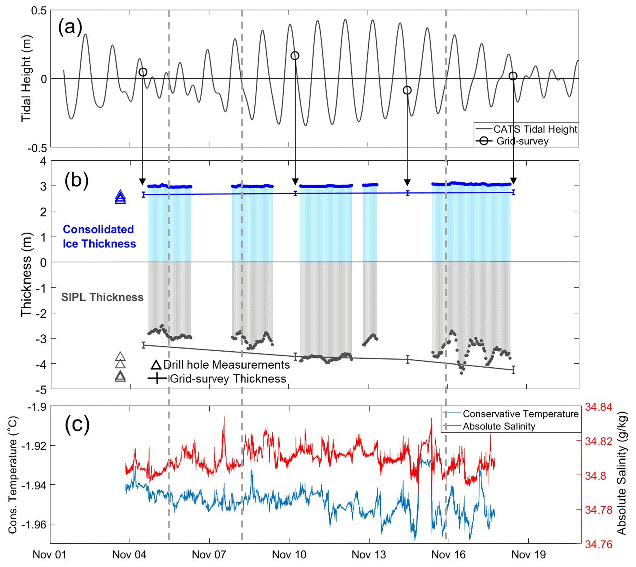
Figure 5(a) CATS tidal height with the times of the repeat grid surveys (circles) shown in (b) as lines of mean EM sea ice and SIPL thickness with standard deviations (vertical bars) plotted with the Spring EM time-series measurements of consolidated ice and SIPL thicknesses and the five drill hole measurements (triangles) of consolidated ice and SIPL thickness made on 3 November 2018. (c) The 101 m depth MicroCAT time series of absolute salinity and conservative temperature from the oceanographic mooring deployed 500 m due north of the Spring site. Stippled vertical lines show the changes in SIPL thickness with the tides on 5, 8, and 16, which are discussed in Sect. 3.1.
3.1.3 Tidal Influence
Significant diurnal variability in SIPL thickness was observed in the Spring EM time series. The stippled vertical lines in Fig. 5 on 5 and 8 November show examples of increases in SIPL thickness (Fig. 5b) occurring on ebb tides during neap and spring tidal ranges. During high spring tidal ranges from 10–12 November, SIPL thickness had both smaller-magnitude increases and decreases. On 16 November, an example of a decrease in SIPL thickness of ∼ 1 m is highlighted in Fig. 5b over a spring flood tide. Indeed, SIPL thickness varied considerably between 15–18 November in correspondence with the oscillation of the tides and as spring tidal ranges decreased in magnitude. To quantify tidal influence, the magnitude of change in I, Q, and inverted SIPL thickness over the tidal range of each flood tide from trough to peak (denoted positive) and ebb tide from peak to trough (denoted negative) during neap and spring cycles was quantified and shown as delta ppm (i.e. magnitude of change over a tidal range) in Fig. 6 with linear fits applied. R2 values of linear fits were 0.53, 0.30, and 0.50 for I, Q, and inverted SIPL thickness, respectively.
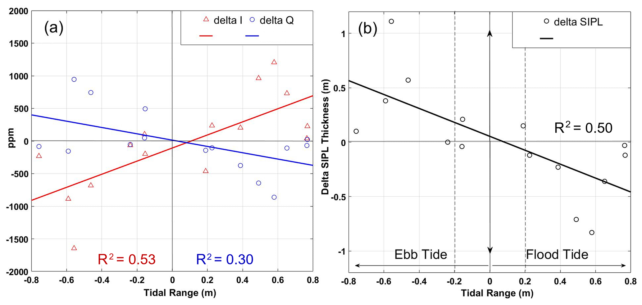
Figure 6The observed magnitude of change in (a) I and Q (delta ppm) and (b) inverted SIPL thickness over the tidal range of each flood from trough to peak (positive) and ebb from peak to trough (negative) tidal range in the Spring EM time series with linear fits and respective R2 values. Stippled vertical lines in (b) delineate neap tidal ranges of ±0.20 m.
Opposing trends were observed in Q and I with the tides (Fig. 6a) where I decreased on ebb tides and increased on flood tides. In contrast, Q increased on ebb tides and decreased on flood tides. Changes in I and Q were largest at maximum ebb tidal ranges of −0.7 m during spring tides. Inverted SIPL thicknesses increased during ebb tides (both spring and neap) (Fig. 6b) and decreased during flood tides, especially during larger-amplitude spring tidal cycles. Neap ebb tides (range of 0.2 m) had on average larger-magnitude increases than decreases in SIPL thickness on flood tides resulting in net overall growth during neap tidal cycles as shown on 5 November in Fig. 5b and by the offset from the origin (0,0) in the linear fit in Fig. 6b. The observed trend of opposing change in I and Q with flood and ebb tides (Fig. 6a) is consistent with forward modelled change in seawater conductivity (Fig. 3a) and inconsistent with forward modelled bulk SIPL conductivity change (Fig. 3b).
3.2 Oceanographic observations
From 3–17 November, the thermistor probes, combined with salinity observed at 101 m depth MicroCAT, showed that the water column was in situ supercooled to a depth of at least 40 m, in agreement with similar observations in this region (Frazer et al., 2020; Stevens et al., 2023). Thus, in situ ice crystal growth and accumulation were supported throughout the Spring EM time series. The 101 m depth MicroCAT time series of absolute salinity and conservative temperature are shown in Fig. 5c. Over the 14 d time series, seawater salinity (conductivity) ranged from 34.80–34.83 g kg−1 (2714–2719 mS m−1) with a maximum change of 0.03 g kg−1 (5 mS m−1) with the tides. Conservative temperature ranged from −1.93 to −1.97 °C with temperature variability broadly corresponding to changes in seawater salinity.
3.3 Temporal variability of the SIPL from repeat EM west–east and grid surveys
Figure 5b also shows mean EM consolidated ice and SIPL thicknesses with standard deviations (error bars) from the 200 m by 200 m grid survey carried out at four occasions on the neap–spring tidal cycle from 4–18 November (Fig. 5a). Mean consolidated ice and SIPL thickness on the grid survey increased by 0.09 m (2.65–2.74 m) and 0.97 m (3.27–4.24 m) over the 14 d neap–spring tidal cycle equating to mean daily growth rates of 0.6 and 7 cm, respectively. Larger increases in SIPL thickness were observed predominately over neap tides between 4 and 10 November and the beginning of neap tides between 14 and 18 November, relative to smaller-magnitude increases observed over spring tides between 10 and 14 November.
Figure 7b shows EM consolidated ice and SIPL thicknesses on the repeated west–east transects across McMurdo Sound, which was fully surveyed with EM on 1 and 19 November and partially surveyed four more times. The colour and time of each survey are displayed on the tidal height curve in Fig. 7a. EM consolidated ice and SIPL thicknesses showed good agreement with drill hole measurements made along the transect between 3 and 19 November. The first survey on 1 November (black) was carried out on a spring flood tide and the last on a neap ebb tide on 19 November (blue) with significant increases in SIPL thickness observed. Over the 18 d survey period, SIPL thickness increased by ∼ 0.6 m in the west (164.8–165.0° E), by ∼ 1.4 m in the centre (165.3–165.6° E), and by ∼ 1.1 m where the Spring site and grid survey were located. This equates to an observed average daily SIPL growth rate of 3 cm in the west, 8 cm in the centre, and 6 cm near the Spring site concurring with the mean SIPL growth rates of the repeat grid surveys (7 cm) and Spring EM time series (7 cm) between 4–18 November.

Figure 7Temporal variability in SIPL thickness on the repeated west–east transect (latitude 77.767° S) (refer to Fig. 1 for location) of EM consolidated ice and SIPL across McMurdo Sound with full surveys carried out on 1 and 19 November and partial surveys on 6, 7, 9, and 13 November (EM surveys on 9 and 13 November are not shown in (b) for clarity). The times of the repeated transects are colour-coded and displayed on the tidal height curve in (a). Drill hole measurements (circles) carried out along the transect between 3–19 November 2018 are also shown. The Spring EM time-series site and grid survey were located at a drill site on the transect at 165.2° E, and the oceanographic mooring was deployed 500 m to the north.
The partial EM transects in November provided additional information on SIPL variability observed at the Spring site and across the sound with respect to the neap–spring tidal cycle between 1 and 19 November. The survey on 6 November (grey) was carried out on a neap ebb tide and showed 0.4–0.6 m of SIPL growth relative to 1 November (black) in the west. This 5 d period between 1 and 6 November was dominated by neap tides. On an ebb tide during the transition from neap to spring cycles on 7 November (red), the SIPL increased substantially relative to the survey on 1 November (black) and had expanded further east. Smaller increases in SIPL thickness were observed on the partial surveys carried out on 9 November (green) (164.8–165.2° E) and 13 November (magenta) (165.2–166.0° E) during spring tides, and these surveys are not shown in Fig. 7b for clarity. The consistency in the EM measured consolidated sea ice thickness in all surveys supports the interpretation of variability in EM measured SIPL thickness over the 18 d survey period.
4.1 Winter evolution of SIPL and temporal variability with strong southerly wind events
The seasonal growth of fast ice and SIPL were captured in the ∼ 7-week Winter EM time series with episodic increases in SIPL thickness co-occurring with strong southerly wind events (Fig. 4). The SIPL began to form in September and persisted from early October. We observed substantial increases in SIPL thickness in the Hut Point Peninsula region during strong southerly wind events, which drove the formation of the McMurdo and Ross Sea polynyas, suggesting a rapid response to wind-driven surface circulation. Brett et al. (2020) observed SIPL thickening of ∼ 1 m in the same region between 13–21 November 2017 which also co-occurred with strong southerly wind events and polynya activity. We speculate whether divergence and upwelling would occur as surface waters are advected offshore by strong southerly winds (Foldvik and Kvinge, 1974). Upwelling could draw water out from beneath the fast ice and out from the ice shelf cavity. The accelerated rise of ISW from deeper in the cavity and decrease in pressure (Foldvik and Kvinge, 1974; Jordan et al., 2015) would promote supercooling and frazil ice formation, which could then be deposited beneath adjacent fast ice. For future winter EM times-series measurement, coincident oceanographic observations are important to determine the mechanisms for rapid increases in SIPL thickness with episodic wind forcing on ocean circulation.
4.2 The influence of the tides on ocean circulation and the SIPL in McMurdo Sound
In the shorter 2-week Spring EM time series, EM inverted SIPL thickness increased on ebb tides (Figs. 5b and 6b) with larger increases observed on spring ebb tides relative to neap ebb tides. However, larger increases on spring ebb tides were negated on spring flood tides when the SIPL thickness decreased by a similar magnitude (Figs. 5b and 6b). During periods of neap tides, larger net growth of SIPL thickness was observed. The same pattern of SIPL thickness increasing more over neap versus spring cycles was observed in the grid surveys (Fig. 5b) and repeat west–east EM transects (Fig. 7b) at the location of the Spring EM time-series site. Increases in SIPL thickness were remarkably similar for the Spring EM time series (0.94 m), the grid survey (0.97 m) over 14 d, and the west–east transect (1.1 m) over 18 d.
A distinct trend emerges of inverted SIPL thickness having larger net overall increases during periods of neap tides relative to spring tides and on diurnal timescales increasing more over ebb tides relative to flood tides. This trend correlates with the tidal current patterns observed in oceanographic studies where neap and spring ebb tides resulted in stronger northward currents (out of the ice shelf cavity) in both east and west McMurdo Sound (Leonard et al., 2011, 2006; Robinson et al., 2010, 2014), which would be comprised of supercooled ISW with a suspension of frazil and platelet ice crystals. Oceanographic observations by Hughes et al. (2014) showed that the depth of in situ supercooling in the centre and east of McMurdo Sound was greater in neap relative to spring tides, which would prime the water column for augmented SIPL growth (Mahoney et al., 2011).
4.3 Potential causes of inverted SIPL thickness variability with the tides
As discussed in Sect. 2.2, EM measures the subsurface bulk conductivity in the form of I and Q, which are then inverted from a three-layer forward model into consolidated ice and SIPL thicknesses. We observed that I decreased on ebb tides and increased on flood tides, and Q increased on ebb tides and decreased on flood tides (Fig. 6a). Considering that the EM measurements are ambiguous and rely on the assumption of specific and constant seawater and SIPL conductivities, we identified three possible causes of variability observed in measured I and Q and resultant inverted SIPL thickness with the oscillation of the tides: (1) change in seawater conductivity, (2) change in SIPL bulk conductivity, or (3) a real physical change in the SIPL thickness. We carried out sensitivity studies of how variability in seawater conductivity and SIPL bulk conductivity would affect I, Q, and inverted SIPL thickness at the Spring site by running multiple forward model scenarios, as described in Sect. 2.2 and shown in Fig. 3. Here we explore the plausibility of 1–3 in consideration of the EM measurements, sensitivity studies, and oceanographic observations.
4.3.1 Seawater conductivity
The trend of opposing change in I and Q with flood and ebb tides fit the pattern of changing seawater conductivity modelled in Sect. 2.2 (Fig. 6a vs. Fig. 3a) (i.e. decreasing seawater conductivity on ebb tides and increasing seawater conductivity on flood tides). However, Fig. 6a shows that seawater conductivity would need to change by a minimum of 150 mS m−1 to account for the change in I and Q with the tides equating to a substantial change in seawater salinity of 1.5 g kg−1. The maximum change in conductivity recorded at the 101 m depth MicroCAT with the tides (Fig. 5c) was 5 mS m−1, corresponding to salinity change of 0.03 g kg−1. Seawater conductivity is thus highly unlikely to have caused the observed change in I and Q and inverted SIPL thickness.
4.3.2 SIPL bulk conductivity
The sensitivity study in Sect. 2.2 demonstrated that increasing and decreasing SIPL bulk conductivity caused concurrent and equal magnitude change in both I and Q, which was not observed in the Spring EM time series (Fig. 6a vs. Fig. 3b). Therefore, it is unlikely that variability in SIPL conductivity with the tides explains the change in EM inverted SIPL thickness. However, for thoroughness, we discuss possible causes and effects of variability in SIPL bulk conductivity. The SIPL is a porous mass of platelet ice crystals with brine-filled interstices. SIPL bulk conductivity could vary with changes in the brine salinity or the solid ice fraction, which could occur with ice formation/melt or brine convection within the layer. However, the SIPL emerges in a mushy layer model to be vertically isothermal with constant brine salinity (Wongpan et al., 2021). These thermohaline properties would make convection within the SIPL weak and inefficient at changing bulk salinity. This would also prevent freezing and consequent change in brine salinity. Although these effects remain to be fully observed, we conclude that a change in SIPL bulk conductivity on diurnal tidal timescales is insufficient to explain the tidal variability in the Spring EM observations.
4.3.3 Change in SIPL thickness
The pattern observed was a consistent increase in SIPL thickness on ebb tides (both spring and neap) and a decrease in thickness on flood tides (Figs. 5b and 6b). Diurnal changes in SIPL thickness could be driven by crystal deposition and growth, movement of masses of SIPL at the base, propagation of ripple-like features at the SIPL–ocean interface analogous to sand dune migration (Robinson et al., 2017), or some combination of these effects. Camera observations of the base of the SIPL in eastern McMurdo Sound (Smith et al., 2012; Leonard et al., 2006) revealed episodic growth bursts of individual platelet ice crystals during neap tides on the order of 1–12 cm d−1. This must contribute to SIPL thickness over long periods of time (i.e. weeks and months), but growth rates of individual platelet crystals seem unlikely to fully account for the rapid response of SIPL thickness to the tides observed within the EM footprint. The movement of masses of SIPL at the base or ripples transported downstream with the currents, as observed by Robinson et al. (2017), could account for rapid changes in SIPL thickness. However, the pattern of change we observed in the EM time-series measurements of SIPL was cyclical (i.e. increasing on ebb tides and decreasing on flood tides in proportion to tidal range), which would not be explained by passing masses of SIPL, which should be more random in occurrence.
Given that northward circulation from the ice shelf cavity is promoted during neap cycles and ebb tides, SIPL thickness increases are most likely caused by enhanced ISW outflow and deposition of frazil and platelet ice crystals from suspension. Video recordings beneath the fast ice in Atka Bay by Hoppmann et al. (2015b) showed a continuous background upward flux of suspended platelet ice crystals with short ∼ 1 h events of very high crystal flux, which they speculate was the main contributor to SIPL growth throughout winter and spring. They observed deposition of the suspended crystals into the porous base of the SIPL, which were frequently resuspended with turbulence and strong currents. Gough et al. (2012) observed frazil and platelet ice crystals in suspension beneath the SIPL in eastern McMurdo Sound to depths of 25 m between 6 June and 20 October 2009. Stevens et al. (2023) observed crystal behaviour with cameras at 1 m beneath the SIPL in the centre-east region of McMurdo Sound. Suspensions of crystals were observed, especially at slack water, with small crystals moving horizontally and larger crystals sometimes seen rising into the SIPL.
In McMurdo Sound, increases of frazil ice density suspended in the upper water column have been observed with supercooled ISW outflow from the cavity (Frazer et al., 2020; Leonard et al., 2006). In Frazer et al. (2020), acoustic profiling of the water column showed that frazil ice suspension was greatest following a tidal current out of the cavity, which correlated with higher levels of supercooling. The modelling of Hughes et al. (2014) showed that higher frazil loads in ISW resulted in higher crystal precipitation rates and SIPL thickening. Similarly, Cheng et al. (2019) modelled multiple vertically modified frazil-laden plumes in McMurdo Sound and found that the SIPL thickening rate is dependent on the vertical distribution of frazil ice concentration and ISW supercooling. This indicates that tidally forced current velocity has complex effects on the mass transport of crystals in suspension, crystal size and trajectory, and rise velocity into the SIPL and requires detailed assessment with respect to SIPL thickness and bulk conductivity.
To summarise, we infer that stronger northward circulation of supercooled ISW out of the McMurdo–Ross Ice Shelf cavity during neap cycles and ebb tides (during both neap and spring cycles) carries a higher density of suspended frazil and platelet ice crystals that are then deposited at the base of the SIPL. To confirm this, future EM time series measurements should be collected with coincident underwater camera footage, observations of ocean properties, current velocities, and acoustic profiling of the water column beneath the SIPL. The induction of the EM field in the SIPL is complex and could vary with spatial and temporal inhomogeneities in the conductive properties or structure of the layer. However, investigations of the properties and structure of the SIPL are inherently difficult to carry out without disturbing its natural state and are thus not well understood. To address this, multi-frequency EM techniques could be applied to better constrain the properties of the SIPL and the response of the EM field to inhomogeneities within the SIPL. Hunkeler et al. (2015) used a multi-frequency EM device and forward modelling techniques to quantify the bulk conductivity and solid ice fraction of the SIPL beneath fast ice in Atka Bay. The method was extended to derive the thickness of the SIPL by applying a drill hole-adjusted geophysical inversion of a three-layer forward model (Hunkeler et al., 2016). Although multi-frequency EM could provide more information on SIPL properties and more detailed resolution of the vertical structure of the SIPL, it requires careful calibration and is more complex, time-consuming, and computationally demanding (Hunkeler et al., 2015).
The late-spring average spatial distributions of Ice Shelf Water-influenced fast ice and sub-ice platelet layer (SIPL) have been well described in McMurdo Sound and compared on interannual timescales in previous studies. However, high-temporal resolution and continuous measurements of fast ice and SIPL evolution on seasonal or diurnal timescales have not been possible due to the significant challenge of collecting frequent in situ measurements, especially in winter. Here, we used an electromagnetic induction instrument deployed on fast ice in McMurdo Sound to capture EM time-series measurements of fast ice and sub-ice platelet thickness in the east in winter and additionally in the west in the main outflow path of Ice Shelf Water (ISW) in late spring. The seasonal evolution of fast ice and SIPL in winter and shorter timescale (episodic and diurnal) variability in SIPL thickness were detected. To investigate the possible processes that could influence SIPL formation, variability observed in SIPL thickness was compared with the occurrence of wind-driven polynya activity during winter and in late spring over shorter diurnal timescales with coincident oceanographic observations and the oscillation of modelled tides.
The winter EM time series successfully captured the seasonal growth of ISW-influenced fast ice and the SIPL in the Hut Point Peninsula region. Substantial increases in SIPL thickness co-occurred with strong southerly wind events and polynya activity in the region in early spring, suggesting wind-enhanced outflow of supercooled ISW from the McMurdo–Ross Ice Shelf cavity. In late spring, EM time-series measurements detected diurnal variability in the thickness of the SIPL, which correlated with the oscillation of the tides. Significant increases in inverted SIPL thickness were observed on ebb tides during both spring and neap cycles with larger net increases during periods of neap tides. This temporal pattern in SIPL variability corresponded with tidal currents recorded in previous oceanographic studies, where ebb tides during both neap and spring tides resulted in northward currents in both eastern and western McMurdo Sound. Northward currents circulate out of the ice shelf cavity and would be comprised of a strong component of supercooled ISW with a suspension of frazil and platelet ice crystals.
We considered how the tides could affect the EM measurement through changing conductive properties of the SIPL and seawater by applying sensitivity studies and considering coincident oceanographic observations. We identified that tidally driven real physical change in SIPL thickness was the most plausible scenario. We conjecture that stronger northward circulation out of the cavity during neap and ebb tides (during both spring and neap cycles) carries a higher density of frazil and platelet ice suspension that is deposited into the base of the SIPL, in agreement with prior modelling and observation studies in McMurdo Sound. Enhanced northward circulation of ISW would also explain the episodic increases in SIPL thickness observed in winter during strong southerly wind events and polynya activity. To identify the exact processes affecting the SIPL on episodic and tidal timescales, future EM time-series measurements should include multi-frequency EM and be collected with dedicated oceanographic moorings and underwater cameras to assess the properties of the SIPL and the ocean circulating beneath.
As discussed in Sect. 2.1, significant temperature drift was observed in the Winter EM time series with large changes in air temperature affecting the EM measurement. Figures A1 and A2 show that air temperature affected Q far more than I with increases in Q correlating with large changes in air temperature that occurred over short time periods (stippled vertical lines show examples in Fig. A1b and d). In spring, the air temperatures were higher in magnitude with a lower observed range (−12 to +7 °C) than during winter. Linear fits of de-trended I and Q versus temperature showed no significant correlation supporting minimal temperature effect in late spring (Fig. A2c and d). Multiple years of field experience with the EM31 instrument in late-spring conditions and the poor linear fits of I and Q versus air temperature gave confidence that the temperature effect was not significant, and no correction was applied.
Figure A1 shows that in winter both I and Q generally decreased as sea ice and SIPL thickness increased over time. For the temperature correction, we removed the growth trend from I and Q before plotting against air temperature (Fig. A2a and b). Linear fits of I and Q versus temperature were applied to obtain an average response across the large range of temperatures observed. We did this for the full EM time-series dataset and separately when no SIPL was present in August and September and in October when SIPL was established. The October EM dataset resulted in the best correction as assessed by linear fits and comparison with drill hole measurements (i.e. after processing the temperature-corrected EM data in the forward model and inversion (Sect. 2.2)). This may be caused by increasing solar elevation and irradiation in October causing a stronger diurnal pattern in air temperature.
As expected, Q had a stronger correlation with air temperature in winter than I (Fig. A2a). The entire winter time series of I and Q were then corrected using their respective equations of the line (Fig. A2). The ratio of Q to I is specific to pairs of consolidated ice and SIPL thickness (Irvin, 2018). Applying separate temperature corrections to Q and I could change the Q–I ratio and result in a poor forward model selection. To assess the temperature corrections applied to I and Q, the raw-uncorrected Q–I and temperature-corrected Q–I ratios are compared in Fig. A1c. The raw-uncorrected and temperature-corrected Q–I ratio values were of similar magnitude with less variability in the temperature-corrected Q–I ratio time series, as was desired.
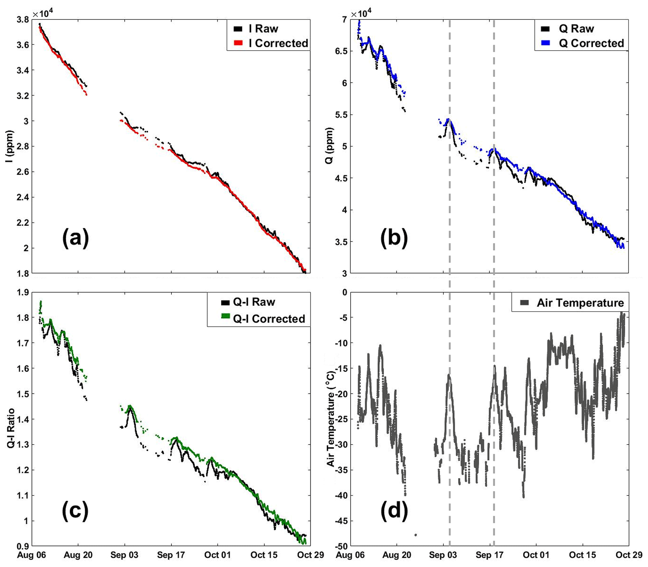
Figure A1Winter EM time-series measurements of raw-uncorrected (black) values with respective temperature-corrected (a) I (red), (b) Q (blue), (c) Q to I ratios (green), and (d) air temperature (grey). Stippled vertical lines in (b) and (d) show examples of raw Q increasing in response to rapid changes in air temperature.
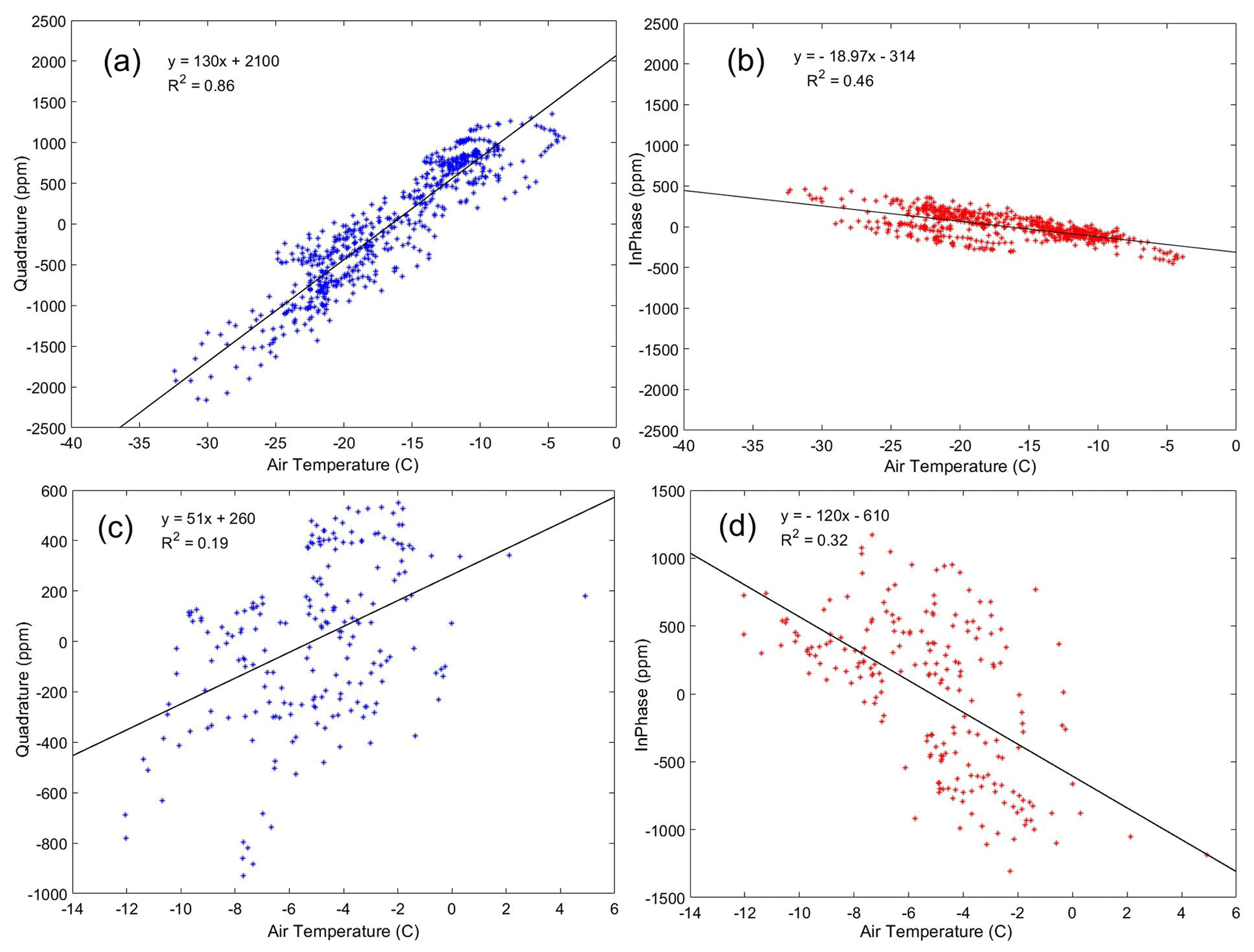
Figure A2Average hourly Q (a, c) and I (b, d), de-trended for the approximately linear growth signal versus air temperature measured by the data logger in winter (a, b) and in late spring (c, d). Lines show linear fits with equations and R2 values.
The drill hole data for 2018 are available at https://doi.org/10.1594/PANGAEA.933050 (Brett et al., 2023), the Winter EM time series at https://doi.pangaea.de/10.1594/PANGAEA.968700 (Brett et al., 2024c), the Spring EM time series at https://doi.pangaea.de/10.1594/PANGAEA.968699 (Brett et al., 2024a), and the west–east EM transects at https://doi.pangaea.de/10.1594/PANGAEA.968701 (Brett et al., 2024b) in the World Data Center PANGAEA (https://www.pangaea.de, last access: 1 October 2023).
GB, GL, and WR modified the EM31 instrument for the winter deployment. GB designed the late-spring fieldwork and GB and GL collected the on-ice field data in November 2018. GB carried out the EM data processing, analyses, and interpretation and wrote the manuscript with input from all co-authors. WR, CH, PL, and AI contributed to the development of the methodology and manuscript. AI developed the EM forward model and inversion technique in collaboration with CH and WR. NR collected and processed all oceanographic data and provided oceanographic expertise.
At least one of the (co-)authors is a member of the editorial board of The Cryosphere. The peer-review process was guided by an independent editor, and the authors also have no other competing interests to declare.
Publisher’s note: Copernicus Publications remains neutral with regard to jurisdictional claims made in the text, published maps, institutional affiliations, or any other geographical representation in this paper. While Copernicus Publications makes every effort to include appropriate place names, the final responsibility lies with the authors.
We thank all contributors of financial and logistical support. We express our deepest gratitude for the invaluable support provided by Scott Base staff and all K063 and K066 field event members, in particular to Inga Smith, Brett Grant, Pete de Joux, and Florence Isaacs. We greatly appreciate the hard efforts of Scott Base winter personnel Sanil Lad and Sam Bamford and to Nick Key and Geoff Graham from the University of Canterbury for their excellent technical support for the first wintertime EM31 deployment. We are very grateful for feedback provided by the editor, Jean-Louis Tison, and the two anonymous reviewers. We acknowledge the use of imagery in our analyses from ESA (available through https://search.asf.alaska.edu, last access: 1 October 2023) and the NASA Worldview application (https://worldview.earthdata.nasa.gov/, last access: 1 October 2023) operated by the NASA/Goddard Space Flight Center Earth Science Data and Information System (EOSDIS) project. Scott Base electronic weather station data were obtained from CliFlo: NIWA's National Climate Database at http://cliflo.niwa.co.nz (last access: 26 August 2019).
This research has been supported by the Ministry of Business, Innovation and Employment (Deep South National Science Challenge: Targeted observations and process-informed modeling of Antarctic sea ice), the University of Canterbury (grant no. Doctoral Scholarship), and Antarctica New Zealand (logistics support under K063 (2018) and K066 (2018) events). The research was carried out in New Zealand at Gateway Antarctica, University of Canterbury, and the University of Otago.
This paper was edited by Jean-Louis Tison and reviewed by two anonymous referees.
Arrigo, K. R., Dieckmann, G., Gosselin, M., Robinson, D. H., Fritsen, C. H., and Sullivan, C. W.: High resolution study of the platelet ice ecosystem in McMurdo Sound, Antarctica: biomass, nutrient, and production profiles within a dense microalgal bloom, Mar. Ecol. Prog. Ser., 127, 255–268, 1995.
Arndt, S., Hoppmann, M., Schmithüsen, H., Fraser, A. D., and Nicolaus, M.: Seasonal and interannual variability of landfast sea ice in Atka Bay, Weddell Sea, Antarctica, The Cryosphere, 14, 2775–2793, https://doi.org/10.5194/tc-14-2775-2020, 2020.
Assmann, K., Hellmer, H., and Beckmann, A.: Seasonal variation in circulation and water mass distribution on the Ross Sea continental shelf, Antarct. Sci., 15, 3–11, 2003.
Barry, J.: Hydrographic patterns in McMurdo Sound, Antarctica and their relationship to local benthic communities, Polar Biol., 8, 377–391, 1988.
Barry, J. and Dayton, P.: Current patterns in McMurdo Sound, Antarctica and their relationship to local biotic communities, Polar Biol. 8, 367–376, 1988.
Brett, G. M., Irvin, A., Rack, W., Haas, C., Langhorne, P. J., and Leonard, G. H.: Variability in the Distribution of Fast Ice and the Sub-ice Platelet Layer Near McMurdo Ice Shelf, J. Geophys. Res.-Oceans, 125, e2019JC015678, https://doi.org/10.1029/2019JC015678, 2020.
Brett, G. M., Price, D., Rack, W., and Langhorne, P. J.: Satellite altimetry detection of ice-shelf-influenced fast ice, The Cryosphere, 15, 4099–4115, https://doi.org/10.5194/tc-15-4099-2021, 2021.
Brett, G. M., Leonard, G. H., Isaacs, F., and Robinson, N. J.: Drill hole measurements of fast ice and sub-ice platelet layer thickness, and snow depth in McMurdo Sound – November 2018, PANGAEA [data set], https://doi.org/10.1594/PANGAEA.933050, 2023.
Brett, G. M., Leonard, G. H., Rack, W., Irvin, A., Haas, C., Langhorne, P. J., and Smith, I.: Winter 2018 time-series measurement of land-fast sea ice and sub-ice platelet layer thicknesses from electromagnetic induction soundings in McMurdo Sound, Antarctica, PANGAEA [data set], https://doi.org/10.1594/PANGAEA.968699, 2024a.
Brett, G. M., Leonard, G. H., Rack, W., Irvin, A., Haas, C., Langhorne, P. J.: Late spring 2018 land-fast sea ice and sub-ice platelet layer thicknesses from electromagnetic induction soundings along repeated west to to east transects in McMurdo Sound, Antarctica, PANGAEA [data set], https://doi.org/10.1594/PANGAEA.968701, 2024b.
Brett, G. M., Leonard, G. H., Rack, W., Irvin, A., Haas, C., Langhorne, P. J., and Smith, I.: Spring 2018 time-series measurement of land-fast sea ice and sub-ice platelet layer thicknesses from electromagnetic induction soundings in McMurdo Sound, Antarctica, PANGAEA [data set], https://doi.org/10.1594/PANGAEA.968700, 2024c.
Cheng, C., Jenkins, A., Holland, P. R., Wang, Z., Liu, C., and Xia, R.: Responses of sub-ice platelet layer thickening rate and frazil-ice concentration to variations in ice-shelf water supercooling in McMurdo Sound, Antarctica, The Cryosphere, 13, 265–280, https://doi.org/10.5194/tc-13-265-2019, 2019.
Dempsey, D. E., Langhorne, P. J., Robinson, N. J., Williams, M. J. M., Haskell, T. G., and Frew, R. D.: Observation and modeling of platelet ice fabric in McMurdo Sound, Antarctica, J. Geophys. Res., 115, C01007, https://doi.org/10.1029/2008jc005264, 2010.
Foldvik, A. and Kvinge, T.: Conditional instability of sea water at the freezing point, Deep-Sea Res. Ocean. Abstr., 21, 169–174, https://doi.org/10.1016/0011-7471(74)90056-4, 1974.
Frazer, E. K., Langhorne, P. J., Leonard, G. H., Robinson, N. J., and Schumayer, D.: Observations of the Size Distribution of Frazil Ice in an Ice Shelf Water Plume, Geophys. Res. Lett., 47, e2020GL090498, https://doi.org/10.1029/2020GL090498, 2020.
Goring, D. G. and Pyne, A.: Observations of sea-level variability in Ross Sea, Antarctica, New Zeal. J. Mar. Fresh., 37, 241–249, 2003.
Gough, A. J., Mahoney, A. R., Langhorne, P. J., Williams, M. J., Robinson, N. J., and Haskell, T. G.: Signatures of supercooling: McMurdo Sound platelet ice, J. Glaciol., 58, 38–50, 2012.
Haas, C.: Comparison of sea-ice thickness measurements under summer and winter conditions in the Arctic using a small electromagnetic induction device, Geophysics, 62, 749, https://doi.org/10.1190/1.1444184, 1997.
Haas, C., Lobach, J., Hendricks, S., Rabenstein, L., and Pfaffling, A.: Helicopter-borne measurements of sea ice thickness, using a small and lightweight, digital EM system, J. Appl. Geophys., 67, 234–241, https://doi.org/10.1016/j.jappgeo.2008.05.005, 2009.
Haas, C., Langhorne, P. J., Rack, W., Leonard, G. H., Brett, G. M., Price, D., Beckers, J. F., and Gough, A. J.: Airborne mapping of the sub-ice platelet layer under fast ice in McMurdo Sound, Antarctica, The Cryosphere, 15, 247–264, https://doi.org/10.5194/tc-15-247-2021, 2021.
Holland, P. R. and Feltham, D. L.: Frazil dynamics and precipitation in a water column with depth-dependent supercooling, J. Fluid Mech., 530, 101–124, 2005.
Hoppmann, M., Nicolaus, M., Hunkeler, P. A., Heil, P., Behrens, L. K., König-Langlo, G., and Gerdes, R.: Seasonal evolution of an ice-shelf influenced fast-ice regime, derived from an autonomous thermistor chain, J. Geophys. Res.-Oceans, 120, 1703–1724, https://doi.org/10.1002/2014jc010327, 2015a.
Hoppmann, M., Nicolaus, M., Paul, S., Hunkeler, P. A., Heinemann, G., Willmes, S., Timmermann, R., Boebel, O., Schmidt, T., and Kühnel, M.: Ice platelets below Weddell Sea landfast sea ice, Ann. Glaciol., 56, 175–190, 2015b.
Hoppmann, M., Richter, M. E., Smith, I. J., Jendersie, S., Langhorne, P. J., Thomas, D. N., and Dieckmann, G. S.: Platelet ice, the Southern Ocean's hidden ice: a review, Ann. Glaciol., 61, 1–28, 2020.
Hughes, K., Langhorne, P., Leonard, G., and Stevens, C.: Extension of an Ice Shelf Water plume model beneath sea ice with application in McMurdo Sound, Antarctica, J. Geophys. Res.-Oceans, 119, 8662–8687, 2014.
Hunkeler, P. A., Hendricks, S., Hoppmann, M., Paul, S., and Gerdes, R.: Towards an estimation of sub-sea-ice platelet-layer volume with multi-frequency electromagnetic induction sounding, Ann. Glaciol., 56, 137–146, https://doi.org/10.3189/2015AoG69A705, 2015.
Hunkeler, P. A., Hoppmann, M., Hendricks, S., Kalscheuer, T., and Gerdes, R.: A glimpse beneath Antarctic sea ice: Platelet layer volume from multifrequency electromagnetic induction sounding, Geophys. Res. Lett., 43, 222–231, https://doi.org/10.1002/2015GL065074, 2016.
Hunt, B. M., Hoefling, K., and Cheng, C.-H. C.: Annual warming episodes in seawater temperatures in McMurdo Sound in relationship to endogenous ice in notothenioid fish, Antarct. Sci., 15, 333–338, 2003.
Irvin, A.: Towards Multi-Channel Inversion of Electromagnetic Sea Ice Surveys, PhD thesis, York University, Toronto, Canada, http://hdl.handle.net/10315/35925 (last access: 4 June 2023), 2018.
Jacobs, S., Helmer, H., Doake, C., Jenkins, A., and Frolich, R.: Melting of ice shelves and the mass balance of Antarctica, J. Glaciol., 38, 375–387, 1992.
Jacobs, S. S., Fairbanks, R. G., and Horibe, Y.: Origin and evolution of water masses near the Antarctic continental margin: Evidence from H218O/H216O ratios in seawater, Oceanology of the Antarctic continental shelf, 43, 59–85, 1985.
Jendersie, S., Williams, M. J., Langhorne, P. J., and Robertson, R.: The density-driven winter intensification of the Ross Sea circulation J. Geophys. Res.-Oceans, 123, 7702–7724, 2018.
Jenkins, A. and Bombosch, A.: Modeling the effects of frazil ice crystals on the dynamics and thermodynamics of ice shelf water plumes, J. Geophys. Res.-Oceans, 100, 6967–6981, 1995.
Jordan, J. R., Kimura, S., Holland, P. R., Jenkins, A., and Piggott, M. D.: On the conditional frazil ice instability in seawater, J. Phys. Oceanogr., 45, 1121–1138, 2015.
Langhorne, P. J., Hughes, K. G., Gough, A. J., Smith, I. J., Williams, M. J. M., Robinson, N. J., Stevens, C. L., Rack, W., Price, D., Leonard, G. H., Mahoney, A. R., Haas, C., and Haskell, T. G.: Observed platelet ice distributions in Antarctic sea ice: An index for ocean-ice shelf heat flux, Geophys. Res. Lett., 42, 5442–5451, https://doi.org/10.1002/2015gl064508, 2015.
Leonard, G. H., Purdie, C. R., Langhorne, P. J., Haskell, T. G., Williams, M. J. M., and Frew, R. D.: Observations of platelet ice growth and oceanographic conditions during the winter of 2003 in McMurdo Sound, Antarctica, J. Geophys. Res.-Oceans, 111, C04012, https://doi.org/10.1029/2005JC002952, 2006.
Leonard, G. H., Langhorne, P. J., Williams, M. J., Vennell, R., Purdie, C. R., Dempsey, D. E., Haskell, T. G., and Frew, R. D.: Evolution of supercooling under coastal Antarctic sea ice during winter, Antarctic Sci., 23, 399–409, 2011.
Lewis, E. L. and Perkin, R. G.: The Winter Oceanography of McMurdo Sound, Antarctica, in: Oceanology of the Antarctic Continental Shelf, edited by: Jacobs, S. S., 145–165, ISBN 9780875901961, https://agupubs.onlinelibrary.wiley.com/doi/abs/10.1029/AR043p0145 (last access: 1 December 2022), 1985.
Lewis, E. and Perkin, R.: Ice pumps and their rates, J. Geophys. Res.-Oceans, J. Geophys. Res., 91, 11756–11762, https://doi.org/10.1029/JC091iC10p11756, 1986.
MacAyeal, D. R.: Thermohaline circulation below the Ross Ice Shelf: A consequence of tidally induced vertical mixing and basal melting, J. Geophys. Res.-Oceans, 89, 597–606, 1984.
Mahoney, A. R., Gough, A. J., Langhorne, P. J., Robinson, N. J., Stevens, C. L., Williams, M. M., and Haskell, T. G.: The seasonal appearance of ice shelf water in coastal Antarctica and its effect on sea ice growth, J. Geophys. Res.-Oceans, 116, C11032, https://doi.org/10.1029/2011JC007060, 2011.
McDougall, T. J. and Barker, P. M.: Getting started with TEOS-10 and the Gibbs Seawater (GSW) oceanographic toolbox, SCOR/IAPSO WG, 127, 1–28, 2011.
McNeil, J.: Technical note TN-6, Electromagnetic terrain conductivity measurement at low induction numbers/Geonics Ltd, 1980.
Ohshima, K. I., Nihashi, S., and Iwamoto, K.: Global view of sea-ice production in polynyas and its linkage to dense/bottom water formation, Geosci. Lett., 3, 13, https://doi.org/10.1186/s40562-016-0045-4, 2016.
Padman, L., Erofeeva, S. Y., and Fricker, H. A.: Improving Antarctic tide models by assimilation of ICESat laser altimetry over ice shelves, Geophys. Res. Lett., 35, L22504, https://doi.org/10.1029/2008GL035592, 2008.
Price, D., Rack, W., Haas, C., Langhorne, P. J., and Marsh, O.: Sea ice freeboard in McMurdo Sound, Antarctica, derived by surface-validated ICESat laser altimeter data, J. Geophys. Res.-Oceans, 118, 3634–3650, 2013.
Price, D., Rack, W., Langhorne, P. J., Haas, C., Leonard, G., and Barnsdale, K.: The sub-ice platelet layer and its influence on freeboard to thickness conversion of Antarctic sea ice, The Cryosphere, 8, 1031–1039, https://doi.org/10.5194/tc-8-1031-2014, 2014.
Price, D., Beckers, J., Ricker, R., Kurtz, N., Rack, W., Haas, C., Helm, V., Hendricks, S., Leonard, G., and Langhorne, P.: Evaluation of CryoSat-2 derived sea-ice freeboard over fast ice in McMurdo Sound, Antarctica, J. Glaciol., 61, 285–300, 2015.
Purdie, C., Langhorne, P., Leonard, G., and Haskell, T.: Growth of first year land-fast Antarctic sea ice determined from winter temperature measurements, Ann. Glaciol., 44, 170–176, 2006.
Rack, W., Haas, C., and Langhorne, P. J.: Airborne thickness and freeboard measurements over the McMurdo Ice Shelf, Antarctica, and implications for ice density, J. Geophys. Res.-Oceans, 118, 5899–5907, https://doi.org/10.1002/2013jc009084, 2013.
Richter, M. E., Leonard, G. H., Smith, I. J., Langhorne, P. J., Mahoney, A. R., and Parry, M.: Accuracy and precision when deriving sea-ice thickness from thermistor strings: a comparison of methods, J. Glaciol., 69, 879–898, https://doi.org/10.1017/jog.2022.108, 2023.
Robinson, N., Williams, M., Barrett, P., and Pyne, A.: Observations of flow and ice-ocean interaction beneath the McMurdo Ice Shelf, Antarctica, J. Geophys. Res.-Oceans, 115, C03025, https://doi.org/10.1029/2008JC005255, 2010.
Robinson, N. J., Williams, M. J. M., Stevens, C. L., Langhorne, P. J., and Haskell, T. G.: Evolution of a supercooled Ice Shelf Water plume with an actively growing subice platelet matrix, J. Geophys. Res.-Oceans, 119, 3425–3446, https://doi.org/10.1002/2013JC009399, 2014.
Robinson, N. J., Stevens, C. L., and McPhee, M. G.: Observations of amplified roughness from crystal accretion in the sub-ice ocean boundary layer, Geophys. Res. Lett., 44, 1814–1822, https://doi.org/10.1002/2016gl071491, 2017.
Robinson, N. J., Grant, B. S., Stevens, C. L., Stewart, C. L., and Williams, M. J. M.: Oceanographic observations in supercooled water: Protocols for mitigation of measurement errors in profiling and moored sampling, Cold Reg. Sci. Technol., 170, 102954, https://doi.org/10.1016/j.coldregions.2019.102954, 2020.
Smith, I. J., Langhorne, P. J., Haskell, T. G., Joe Trodahl, H., Frew, R., and Ross Vennell, M.: Platelet ice and the land-fast sea ice of McMurdo Sound, Antarctica, Ann. Glaciol., 33, 21–27, 2001.
Smith, I. J., Langhorne, P. J., Frew, R. D., Vennell, R., and Haskell, T. G.: Sea ice growth rates near ice shelves, Cold Reg. Sci. Technol., 83–84, 57–70, https://doi.org/10.1016/j.coldregions.2012.06.005, 2012.
Stern, A., Dinniman, M., Zagorodnov, V., Tyler, S., and Holland, D.: Intrusion of warm surface water beneath the McMurdo Ice Shelf, Antarctica, J. Geophys. Res.-Oceans, 118, 7036–7048, 2013.
Stevens, C., Robinson, N., O'Connor, G. and Grant, B.: Ocean turbulent boundary-layer influence on ice crystal behaviour beneath fast ice in an Antarctic ice shelf water plume: The “dirty ice”, Front. Mar. Sci., 10, 1103740, https://doi.org/10.3389/fmars.2023.1103740, 2023.
Wongpan, P., Vancoppenolle, M., Langhorne, P. J., Smith, I. J., Madec, G., Gough, A. J., Mahoney, A. R., and Haskell, T. G.: Sub-Ice Platelet Layer Physics: Insights From a Mushy-Layer Sea Ice Model, J. Geophys. Res.-Oceans, 126, e2019JC015918, https://doi.org/10.1029/2019JC015918, 2021.