Past and future of the Arctic sea ice in High-Resolution Model Intercomparison Project (HighResMIP) climate models

We examine the past and projected changes in Arctic sea ice properties in six climate models participating in the High-Resolution Model Intercomparison Project (HighResMIP) in the Coupled Model Intercomparison Project Phase 6 (CMIP6). Within HighResMIP, each of the experiments is run using a reference resolution configuration (consistent with typical CMIP6 runs) and using higher-resolution configurations. The role of horizontal grid resolution in both the atmosphere model component and the ocean model component in reproducing past and future changes in the Arctic sea ice cover is analysed. Model outputs from the coupled historical (hist-1950) and future (highres-future) runs are used to describe the multi-model, multi-resolution representation of the Arctic sea ice and to evaluate the systematic differences (if any) that resolution enhancement causes. Our results indicate that there is not a strong relationship between the representation of sea ice cover and the ocean/atmosphere grids; the impact of horizontal resolution depends rather on the sea ice characteristic examined and the model used. However, the refinement of the ocean grid has a more prominent effect compared to the refinement of the atmospheric one, with eddy-permitting ocean configurations generally providing more realistic representations of sea ice area and sea ice edges. All models project substantial sea ice shrinking: the Arctic loses nearly 95 % of sea ice volume from 1950 to 2050. The model selection based on historical performance potentially improves the accuracy of the model projections and predicts that the Arctic will turn ice-free as early as 2047. Along with the overall sea ice loss, changes in the spatial structure of the total sea ice and its partition in ice classes are noticed: the marginal ice zone (MIZ) will dominate the ice cover by 2050, suggesting a shift to a new sea ice regime much closer to the current Antarctic sea ice conditions. The MIZ-dominated Arctic might drive development and modification of model physics and parameterizations in the new generation of general circulation models (GCMs).

1 Introduction

Sea ice is the key feature of high-latitude climate through its role in the surface energy budget, ocean and atmosphere dynamics, and marine ecosystems. Over recent decades, the Arctic has witnessed unprecedented sea ice loss, which is a key indicator of global climate change (e.g. Onarheim et al., 2018; Serreze and Meier, 2019), driven by both anthropogenic activities and internal climate variability (e.g. Notz and Stroeve, 2016). Arctic sea ice has declined in every month of the year, with the strongest trends in September: a sea ice extent (SIE) reduction of 7.9×10⁴ km² yr⁻¹ in the period 1979–2022 compared to that in March, 3.92×10⁴ km² yr⁻¹, in 1979–2022 (http://nsidc.org/arcticseaicenews/2022/, last access: 4 June 2024). The overall decrease in SIE reveals large seasonal and regional variability. Although winter sea ice loss is dominated by the reduction in the Barents Sea (Årthun et al., 2021), the most pronounced summer sea ice decreases occur in the East Siberian Sea (explaining more than 20 % of the September trend; Watts et al., 2021) and in the Beaufort, Chukchi, Laptev and Kara seas (Onarheim et al., 2018). Along with a severe reduction in sea ice coverage, Arctic sea ice has also thinned, with a ∼ 70 % reduction in summer sea ice volume (SIV) from 1979 to 2021 (https://nsidc.org/, last access: 4 June 2024). As a consequence, the Arctic ice is getting younger: the proportion of multi-year ice, which previously was the iconic feature of the Arctic in winter months, has decreased from ∼ 30 % in 1985 (the beginning of the satellite era) to ∼ 4.4 % in 2020 (Perovich et al., 2020). The Arctic transition toward a first-year-ice regime might substantially alter the interactions in the ocean–atmosphere–ice system (Aksenov et al., 2017). The changes in total SIE and in sea ice thickness (SIT) cause a redistribution of the sea ice classes; in particular, the marginal ice zone (MIZ) is strongly affected (Rolph et al., 2020). The Arctic MIZ holds interest as it is the fundamental region supporting many physical, biological, and biogeochemical processes (Galí et al., 2021). The MIZ is traditionally defined as the region where polar air, ice, and water masses interact with the ocean temperature and subpolar climate system (Wadhams and Deacon, 1981). It corresponds to the portion of the ice-covered ocean often characterized by highly variable ice conditions, where surface gravity waves significantly impact the dynamics of sea ice (e.g. Dumont et al., 2011). Due to the large uncertainties in observed and forecasted waves within sea ice, the MIZ is still operationally defined through sea ice concentration (SIC) thresholds as the transition zone between open water and consolidated pack ice, where the total area of the ocean is covered by 15 %–80 % sea ice (e.g. Strong et al., 2017; Paul et al., 2021; Rolph et al., 2020). While there have been no significant changes in the area of the Arctic MIZ during the satellite era (Rolph et al., 2020), the marginal ice zone fraction (MIZF), defined as the percentage of total sea ice area (SIA) covered by MIZ (Horvat, 2021), increases by more than 50 % in August and September as the total SIA decreases drastically (Rolph et al., 2020; Horvat, 2021). Since the MIZ differs from the pack ice in higher sensitivity to the dynamic and thermodynamic forces, the growing MIZF changes the Arctic response to global warming, which may worsen the pace of sea ice melt and cause repercussions for local and global climate.

Assuming that the Arctic Ocean will continue to lose sea ice, a relevant question is how fast the Arctic will turn ice-free in summer. Coupled climate models can be used in the prediction and projection of the climate system, including the sea ice conditions. In the majority of simulations from CMIP6 (Eyring et al., 2016), the Arctic Ocean becomes practically sea-ice-free (SIA < 1×10⁶ km²) in September in all scenarios for the first time before 2050 (Notz and SIMIP Community, 2020) or even by 2035 when selecting only the models that best represent the present Arctic sea ice state and northward ocean heat transport (Docquier and Koenigk, 2021). Even using a process-based selection criterion, uncertainties in the model projections are relatively large, which undermines the model's trustworthiness (Docquier and Koenigk, 2021). Besides, the accurate simulation of past and present Arctic sea ice is still challenging. Although the CMIP6 multi-model ensemble mean is closer to the observed sensitivity of Arctic sea ice to global warming (Notz and SIMIP Community, 2020; Shu et al., 2020), there is little difference in overall model performance among CMIP3, CMIP5, and CMIP6. CMIP6 models still simulate a wide spread of mean sea ice area and volume in March and September (Davy and Outten, 2020; Notz and SIMIP Community, 2020; Watts et al., 2021).

Among the model developments and improvements needed to produce more accurate future projections, increasing horizontal spatial resolution is recognized to be a key step in enhancing the representation of the complex processes at high latitudes and in obtaining trustworthy projections of ice variability. In order to address the impact of the model grid resolution on the simulated oceanic and atmospheric phenomena, the High-Resolution Model Intercomparison Project (HighResMIP; Haarsma et al., 2016) was designed within the EU Horizon 2020 PRIMAVERA project (PRocess-based climate sIMulation: AdVances in high-resolution modelling and European climate Risk Assessment, https://www.primavera-h2020.eu/, last access: 4 June 2024). HighResMIP is one of the CMIP6-endorsed model intercomparison projects, which provides a useful framework to investigate the role of enhanced horizontal resolution in representing the features of the climate system. A number of climate modelling groups contributed to the project, providing the same simulations in at least two different configurations. The impact of the increased resolution within the HighResMIP is examined in many studies with regard to the atmosphere, sea ice, and ocean components of the climate systems (e.g. Fuentes-Franco and Koenigk, 2019; Docquier et al., 2019; Bador et al., 2020; Roberts et al., 2020; Jackson et al., 2020; Lohmann et al., 2021; Meccia et al., 2021). Even though high-resolution models can resolve specific dynamical features, the role of the enhanced horizontal resolution is not uniform across ocean regions and models. Grist et al. (2018) demonstrated that refining the ocean grid to eddy-permitting resolution raises the Atlantic meridional heat transport and improves agreement with observational estimates – they also show the significantly smaller impact of atmosphere resolution on the strength of the heat transport. Docquier et al. (2019) confirmed this finding and showed that a better representation of Atlantic surface characteristics, velocity fields, and sea surface temperature (in addition to transports toward the Arctic) improves the representation of the Arctic SIA and SIV. Nevertheless, the role of ocean resolution in the representation of ocean heat transport (OHT) and SIA is less clear when considering the regional effect on specific Arctic sectors, as shown for the Barents Sea in Docquier et al. (2020).

Here, we focus on the impact of horizontal resolution on the Arctic sea ice properties in the past and future at hemispheric and regional scales using the model outputs from coupled historical (hist-1950) and future (highres-future) runs in HighResMIP. We assess seasonal and interannual variability and trends in the SIA and SIV and examine when the Arctic will see its first ice-free summer. We aim to explore the role of enhanced ocean/atmosphere horizontal resolution in the representation of past and current sea ice and to provide some insight into whether the grid refinement improves the model performance in predicting future Arctic sea ice conditions.

2 Data

In this study, we analyse the outputs from the six coupled climate models participating in the HighResMIP. We use coupled runs with historical forcing (hist-1950) covering the period of 1950–2014 and future projections (highres-future) from 2015 to 2050 based on the fossil-fuelled development SSP5-8.5 scenario. For the ocean, five models use different versions of the Nucleus for European Modelling of the Ocean framework (NEMO, Madec et al., 2016), whereas MPI-ESM is based on the Max Planck Institute Ocean Model (MPIOM; Jungclaus et al., 2013). The basic characteristics of the models are given in Table 1. Because each model uses at least two different resolutions, we evaluate 14 configurations in total. CMCC-CM2 and MPI-ESM use one ocean (eddy-permitting) resolution with two different atmospheric grids. ECMWF-IFS and EC-Earth3P run two of three configurations with an eddy-permitting ocean and different atmosphere resolutions. In other models, ocean and atmosphere resolutions vary in concert among configurations. ECMWF-IFS is not considered in the analysis of future projections since it does not provide the outputs from highres-future experiments. It is important to note that ECMWF-IFS, EC-Earth3P, and CNRM benefit from several ensemble members (eight, three, and six members for ECMWF LR, MR, and HR, respectively, and three members for both configurations of EC-Earth3P and CNRM). Given the small ensemble size of multi-ensemble configurations, a clear assessment of internal variability is not feasible in the context of this paper. We use only the first ensemble member in this study. For the past sea ice properties, we mainly focus on the time period beginning in 1979 to compare model results with available satellite records. The simulated SIA is validated against satellite observations. We use monthly SIC from two satellite-based products: the NOAA/NSIDC Climate Data Record (version 4; Meier et al., 2021, hereafter CDR) and the European Organisation for the Exploitation of Meteorological Satellites (EUMETSAT) Ocean and Sea Ice (OSI) Satellite Application Facility (SAF) Climate Data Record and Interim Climate Data Record (release 2, products OSI-450 and OSI-430-b; Lavergne et al., 2019) for the period 1979–2021. CDR uses gridded brightness temperatures in low frequencies from the Nimbus-7 Scanning Multichannel Microwave Radiometer (SMMR; 18 and 37 GHz) and the Defense Meteorological Satellite Program (DMSP) series of Special Sensor Microwave Imager (SSM/I) and Special Sensor Microwave Imager/Sounder (SSMIS) instruments (19.4, 22.2, and 37 GHz). Different ratios of frequencies are used to filter weather effects. The output data are distributed on a 25 km × 25 km polar stereographic grid. The CDR algorithm blends the NASA Team (NT; Cavalieri et al., 1984) and the Bootstrap algorithms (BT; Comiso, 1986) by selecting the higher concentration value for each grid cell, thus taking advantage of the strengths of each algorithm to produce concentration fields that are more accurate than those from either algorithm alone (Meier et al., 2014). OSI SAF comprises two SIC products based on passive microwave sensors: OSI-450 (from 1979 to 2015) and the OSI-430-b extension from 2016 onwards. OSI-450 uses data from the SMMR (1979–1987), SSM/I (1987–2008), and SSMIS (2006–2015) instruments (19.35 and 37 GHz frequencies) together with Era Interim reanalysis (Dee et al., 2011), while OSI-430-b is based on SSMIS and operational analysis and forecasts from the ECMWF. We use estimates of SIT and SIV from the Pan-Arctic Ice Ocean Modeling and Assimilation System (PIOMAS; Zhang and Rothrock, 2003) that comprise the global Parallel Ocean and sea Ice Model (POIM) coupled to an eight-category thickness and enthalpy distribution sea ice model and a data assimilation of sea surface temperature (SST from NCEP/NCAR reanalysis; Kalnay et al., 1996) and SIC (from the National Snow and Ice Data Center, NSIDC, near-real-time product; Brodzik and Stewart, 2016). PIOMAS proved its credibility versus in situ measurements (Stroeve et al., 2014; Wang et al., 2016), and therefore it is widely used in numerous intercomparison studies as the observational proxy (e.g. Labe et al., 2018). Note that PIOMAS tends to underestimate the thick ice north of Greenland and the Canadian Arctic Archipelago and to overestimate SIT in the areas of thin ice (Stroeve et al., 2014; Wang et al., 2016). Monthly fields of SIC and effective SIT from 1979 to 2021 are used in this work. We describe sea ice coverage in terms of SIA (the integral sum of the product of ocean grid-cell areas and the corresponding sea ice concentration) instead of SIE (the integral sum of the areas of all grid cells with at least 15 % SIC). To compute SIV, the equivalent SIT (the sea ice volume per grid cell) is multiplied by the area of the individual grid-cell and then summed over the Arctic region. To derive integrative metrics, only the grid cells with at least 15 % SIC are considered, owing to the high uncertainty in passive microwave retrievals in low-sea-ice conditions. Apart from model evaluation at the hemispheric scale, we provide a regional analysis of sea ice variability in six subregions of the Arctic Ocean (north of 65° N), as defined in Fig. 1.

Table 1 Models and specifications of the configurations used in this study.

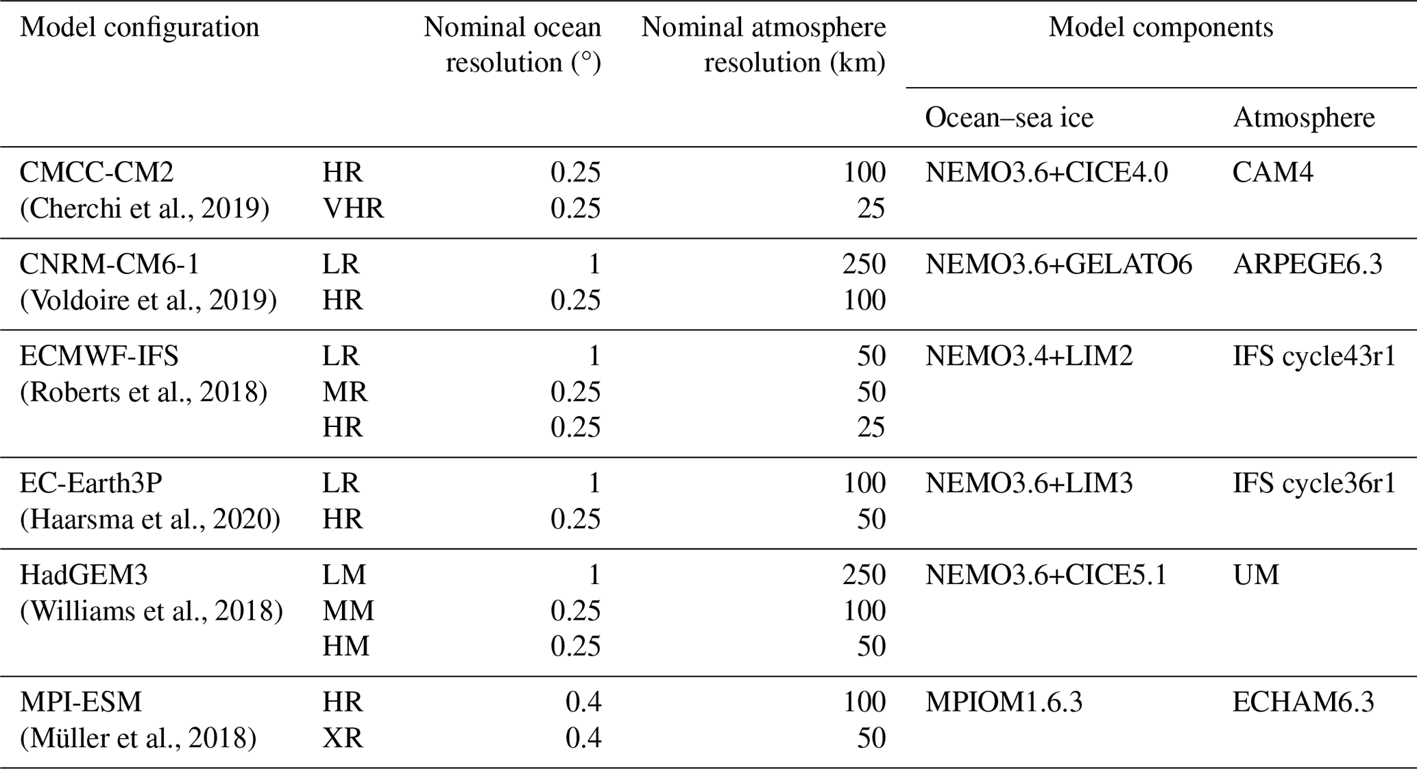
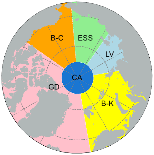
Figure 1 Map of the sub-regions used in the regional analysis: central Arctic Basin (CA), Barents–Kara seas (B-K), Laptev Sea (LV), East Siberian Sea (ESS), Beaufort–Chukchi seas (B-C), and Canadian Arctic Archipelago and Greenland coast (GD).

3 Results

3.1 Mean state

First, we assess the spatial patterns of simulated ice properties against observation-based estimates over the historical period restricted to 1979–2014. Figure 2 shows the climatological mean distribution of SIT in March and September for model outputs and PIOMAS. The mean position of 15 % and 80 % of the SIC edges from each model and CDR (over PIOMAS) is also shown. In general, most models struggle to reasonably simulate the spatial pattern of SIT and produce either thicker (ECMWF-IFS, EC-Earth3P, and CMCC-CM2 VHR4) or thinner (CNRM-CM6 and MPI-ESM) ice over a vast area compared to PIOMAS. Some models are able to correctly locate the thickest ice north of Greenland and the Canadian Arctic Archipelago and the thinner ice in the Siberian Shelf seas (HadGEM3 and CMCC-CM2 HR4), but the simulated ice can thicken up to 7 m. EC-Earth3P HR and ECMWF-IFS MR, despite capturing the overall SIT pattern, also simulate high thickness in the East Siberian and Chukchi seas, which is clearly visible in March. This might be related to unrealistic sea ice drift. As in PIOMAS, most models reproduce changes in the SIT between March and September showing a more pronounced seasonal retreat in the Siberian sector.

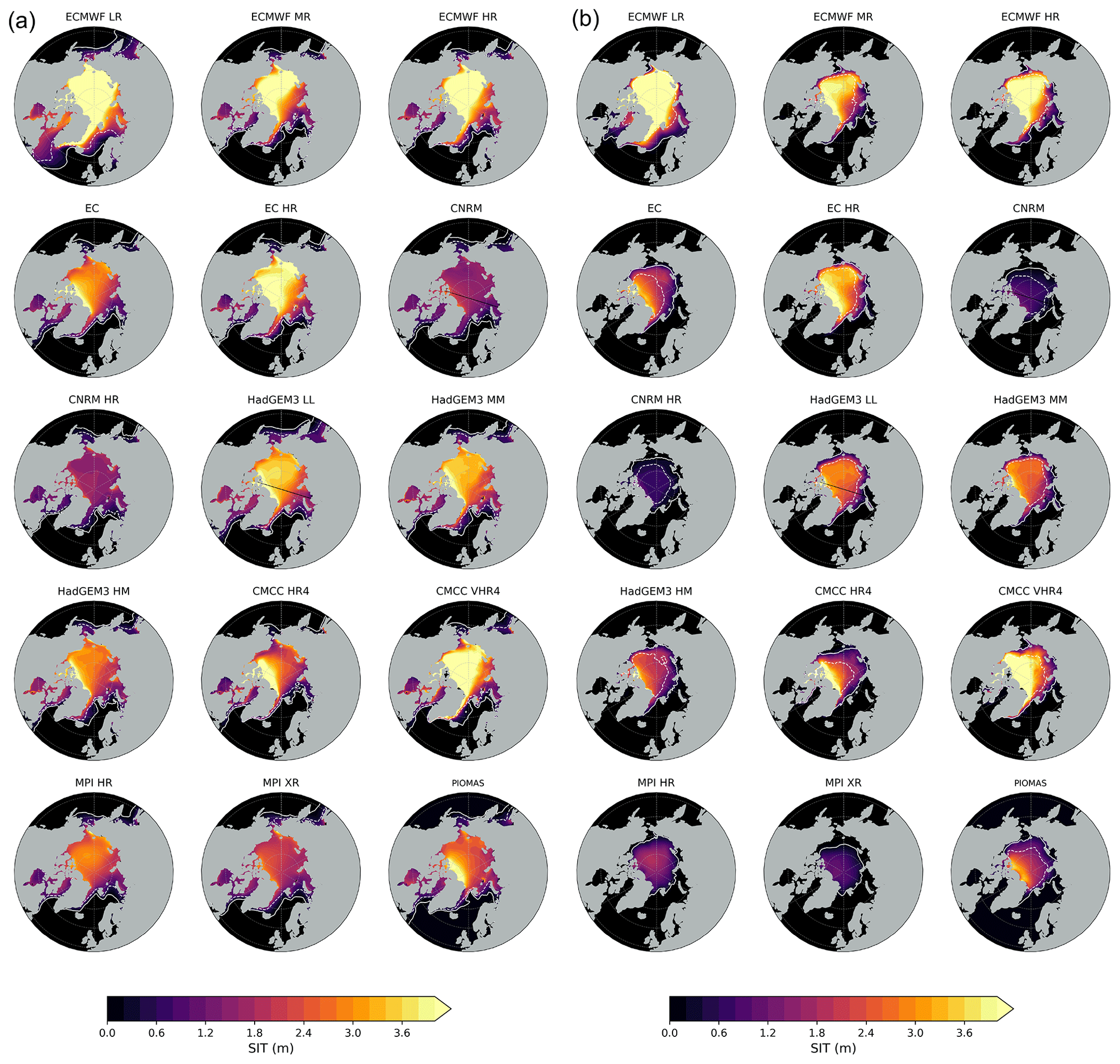
Figure 2 The 1979–2014 climatological mean sea ice thicknesses from the model outputs and from PIOMAS in March (a) and September (b). White contours show the edges of 15 % (solid) and 80 % (dashed) sea ice concentrations from each model. SIC from CDR is used for PIOMAS.

There is no direct effect of horizontal resolution on the spatial distribution of SIT. When the ocean resolution is increased, the mean SIT decreases for ECMWF-IFS, does not change notably for HadGEM3 and CNRM-CM6, and increases for EC-Earth3P. The role of atmosphere resolution also depends on the model; for example, the finer-atmosphere-resolution MPI-ESM reproduces on average slightly thinner ice compared to the LR configuration, while the finer CMCC-CM2 simulates thicker ice over a larger area. Biases in the representation of SIT pattern can be related to poor representation of surface pressure and large-scale atmospheric patterns (Kwok and Untersteiner, 2011; Stroeve et al., 2014), sea ice motion, and ocean forcing (Watts et al., 2021).

Most models tend to realistically simulate the position of the sea ice edge in both March and September. The LR configuration of ECMWF-IFS tends to overestimate the sea ice cover in the far south of the North Atlantic and North Pacific oceans compared to CDR. The bias can be explained by the poor representation of the ocean advection. Docquier et al. (2019) showed that the northward OHT is improved when the ocean resolution increases from 1 to 0.25°, both across the Bering Strait (83 km wide) and through the Nordic seas, establishing the Atlantic warm inflow into the Arctic Ocean. Similarly for SIT, the effect of the atmospheric grid resolution on the sea ice extent is model dependent. When it is enhanced, there are no notable changes in the location of the March ice edge in the ECMWF-IFS and HadGEM3 models, but it is largely overestimated in CMCC-CM2 and MPI-ESM, particularly in the Nordic seas. Specifically, CMCC-CM2 HR4 underestimates March sea ice coverage in the northern Barents Sea, the Bering Sea, and the Sea of Okhotsk, whereas the VHR4 version (with a finer atmospheric grid) reproduces a reasonable amount of winter ice in marginal seas. In September, higher atmosphere resolution leads to a larger SIA in ECMWF-IFS and CMCC-CM2; conversely it has the opposite effect in the HadGEM3 and MPI-ESM models. In addition, MPI-ESM XR significantly melts sea ice in the Siberian seas, which are almost ice-free in summer. The width of the MIZ (marked in Fig. 2 by the area between 15 % and 80 % SIC contours) also varies among different models. In many of them, March MIZ surrounds the inner ice pack in a similar way, comparing well with CDR. In September, most models simulate an extension of MIZ that is fairly comparable to the observed one. Exceptions are the MPI-ESM runs that lose all consolidated pack ice in summer and ECMWF LR runs that tend to overestimate the total and pack ice, with a small portion covered by marginal ice in the Barents Sea and Nordic seas.

3.2 Seasonal variability

Figure 3 shows the mean seasonal cycle of the total Arctic SIA and SIV computed over the 1979–2014 period. Satellite estimates from both OSI SAF and CDR are included to validate the model outputs. The CDR Arctic ice area expands to its maximum in March, with coverage of nearly 14×10⁶ km², and returns to its minimum in September at around 6×10⁶ km². Similar seasonality is displayed by the OSI SAF dataset, which has a slightly smaller SIA in all months.

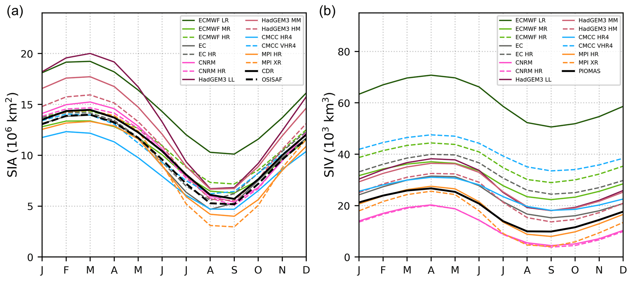
Figure 3 The 1979–2014 seasonal cycle in SIA (a) and SIV (b) from HighResMIP hist-1950 model outputs versus CDR and OSI SAF for SIA and versus PIOMAS for SIV.

As in the CMIP5 and CMIP6 low-resolution models (Shu et al., 2020; Notz and SIMIP Community, 2020), most HighResMIP models adequately reproduce the mean seasonal cycle of SIA, with the melt season starting in March and lasting until September when a minimum is reached (Fig. 3a). There is a considerable spread among models; it is relatively larger in winter than in summer. March SIA ranges from 12 to 20×10⁶ km², while September values lie in the range between 3 and 7.5×10⁶ km² in all but one model. The ECMWF-ISF LR overestimates the Arctic SIA all year round, but it can properly represent the amplitude of SIA seasonal variability and hence correctly reproduces the ice advance and retreat phases. The comparison between the model configurations indicates that finer resolution generally results in a simulated SIA closer to satellite products. The effect of changing atmosphere resolution varies among models, however. For instance, the CMCC-CM2 HR constantly stays in the lower bound of the model ensemble and reproduces a weaker amplitude of the seasonal cycle compared to observations; applying the atmospheric grid refinement (CMCC-CM2 VHR4 configuration) favourably increases sea ice coverage and does not significantly change the seasonal cycle amplitude. A different impact is observed for the MPI-ESM model: the finer atmospheric grid leads to closer agreement with observations in SIA during winter but increases the spring/summer melting, resulting in an underestimated September minimum of up to ∼ 50 % compared to observations. In general, in other HighResMIP runs, the atmosphere grid refinement gives smaller changes to Arctic sea ice coverage compared to the ocean resolution enhancement. In the ECMWF-IFS, the LR shows a constant SIA overestimation that is largely resolved in the model configuration with an eddy-permitting ocean (HR), particularly in summer. The same behaviour is seen for six ECMWF ensemble members (Fig. S1 in the Supplement). As for the CMCC-CM2 model, a further refinement in the atmosphere resolution increases the SIA in the whole year, with the best agreement with observations from October to July. The HadGEM3 runs are relatively close to observations in summer, but they tend to overestimate the sea ice growth – the impact of increased ocean and atmosphere resolution is evident for this model, with a strong reduction in winter sea ice of ∼ 25 % from LL to HM and a smaller but still remarkable contraction in summer. Here, the increase in the atmosphere resolution further reduces SIA in contrast to previous models. Finally, the EC-Earth3P and CNRM-CM6 models show negligible differences between model configurations, regardless of ocean and atmosphere grid resolutions.

In our reference product, PIOMAS, the Arctic SIV ranges from ∼ 25×10³ km³ at its peak in April to ∼ 10×10³ km³ at its minimum in August/September (Fig. 3b). All models capture the timing of the SIV maximum in April and the minimum in August/September, with a realistic seasonal cycle amplitude that ranges between 15 and 20×10³ km³. However, there is a large spread among different models, with most models overestimating PIOMAS–ECMWF-ISF LR is a clear outlier, exceeding 70×10³ km³ in April and 50×10³ km³ in September. Although in some models the bias in SIA is seasonally dependent, with larger errors in winter, the bias in simulated SIV is consistent throughout the year in all models. In general, large SIV is mainly due to poorly simulated SIT rather than incorrect sea ice cover (Figs. 2 and 3a). Only in ECMWF-IFS LR does the combination of large ice expansion and extremely thick ice lead to unrealistically high SIV. The SIV overestimation in the CMCC-CM2 and EC-Earth3P models is caused by the sea ice being too thick, even though their SIAs compare well with observations. Only one model (CNRM-CM6 in both configurations) has thin ice and hence low bias in SIV compared to PIOMAS all year round. The changes in resolution have no visible impact in this case. The increase in only ocean resolution largely improves the representation of SIV (the same for SIA) in ECMWF-IFS with a large volume reduction (including six ensemble members; Fig. S1) but does not affect the volume seasonality in HadGEM3. Finer atmosphere resolution and the combined resolution increases tend to increase the ice volume, except in HadGEM3 and MPI-ESM. MPI-ESM has a good fit to PIOMAS for SIV, although this model underestimates SIA and cannot simulate consolidated pack ice (SIC > 80 %, Fig. 2).

In addition to the total SIA, we show the seasonal variability in the area covered by marginal ice over the same 1979–2014 period (Fig. 4a). It is worth noting that the evaluation of the simulated MIZ area is highly dependent on the reference product used, particularly in summer. This can be mainly ascribed to the treatment of wet surfaces (e.g. melt ponds and snow wetness) that causes difficulty in retrieving the SIC using passive microwave radiometers (Ivanova et al., 2015). OSI SAF has a small portion of MIZ in winter, but it overestimates CDR from May to November. The maximum difference between the two products increases to nearly 0.9×10⁶ km² in July. The observed MIZ seasonal variability contrasts with that shown by the total ice area: the MIZ expands in spring when the consolidated pack ice starts to melt, and this process leads to the MIZ area peak occurring in summer. After reaching its maximum in July, the marginal ice starts to melt and its area decreases with the total and consolidated pack ice cover simultaneously until September. Before the next year's melting season, the MIZ stays relatively stable, but with a secondary peak in October at the beginning of sea ice advance. The models are overall able to simulate the seasonal cycle, reasonably capturing the phases of the MIZ expansion and retreat. However, they tend to overestimate the MIZ in winter, but most of their estimates lie between the OSI SAF and CDR summer estimates. Generally, models struggle to properly simulate the timing and magnitude of the MIZ maximum. ECMWF-IFS LR is higher than observations from November to May due to a large overestimation of the total ice area; nevertheless, it lies between CDR and OSI SAF during the rest of the year. Noteworthy, the ECMWF-IFS finer-resolution configurations are in better agreement with observed values. In the HadGEM3 LL configuration, the marginal ice expansion starts earlier, with a large bias in the MIZ area from March to June. Increasing resolution in the HadGEM3 model does not have a visible impact on the rest of the year. The impact of changes in the ocean and atmosphere resolution is small in other models. Finally, MPI-ESM configurations fail to reproduce the MIZ seasonal cycle from June to November. This pairs with Fig. 2, which shows underestimation of consolidated pack ice and MIZ predominance in the MPI-ESM runs.

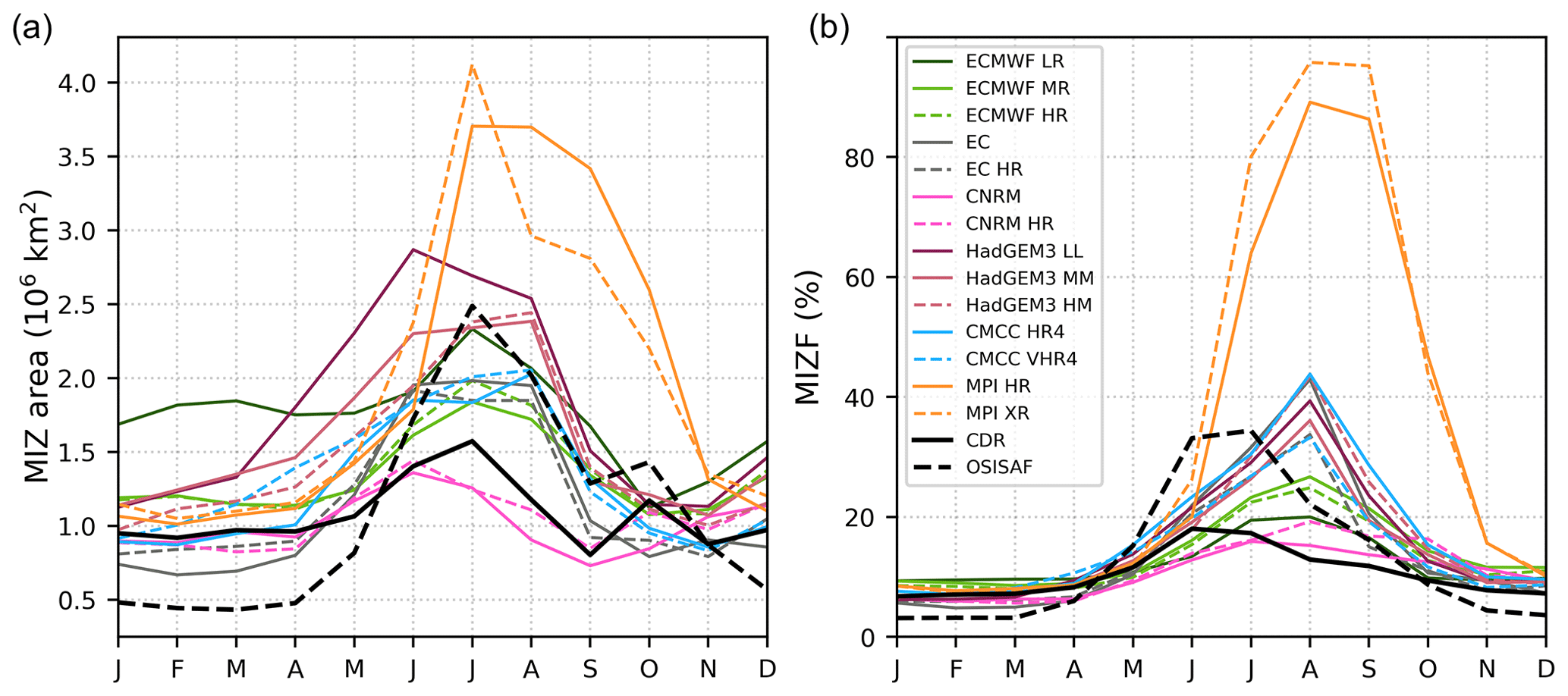
Figure 4 The 1979–2014 seasonal cycle in the MIZ area (a) and MIZF percentage (b) from HighResMIP hist-1950 model outputs and satellite products.

We also show the seasonal cycle of the MIZ area fraction (MIZF) from 1979 to 2014, calculated from model and satellite product outputs (Fig. 4b). The MIZF is defined as the percentage of the ice cover that is MIZ (Horvat, 2021) and reflects the relative changes in the MIZ, which are highlighted since the total ice experiences substantial seasonal variability. The observed MIZF ranges from about 5 %–10 % in winter to about 20 %–40 % at its maximum between June/July. For all models, the simulated MIZF maxima are delayed compared to the satellite estimates and to the MIZ area by about 1 month, when the total ice area approaches the September minimum, and the MIZ area is still large. Notably, the HighResMIP models are in better agreement with observations when considering the MIZF rather than the MIZ area. Excluding the MPI-ESM configurations, all models are in general agreement from November to May; the model spread enlarges in spring/summer but the models lie within the observation envelope regardless. The use of the MIZF metric highlights the peculiar representation of Arctic sea ice in the MPI-ESM: up to 95 % of sea ice in the model consists of marginal ice.

3.3 Seasonal variability in the sub-regions

Since sea ice changes in the Arctic region are not uniform in space and time as a result of local climate effects (Parkinson et al., 1999; Meier et al., 2007; Peng and Meier, 2018), it is important to also monitor the sea ice change on regional scales. We analyse the seasonal variability in SIA and SIV in six sub-regions, and we compare it with that of reference products (Fig. 5, Table 2).

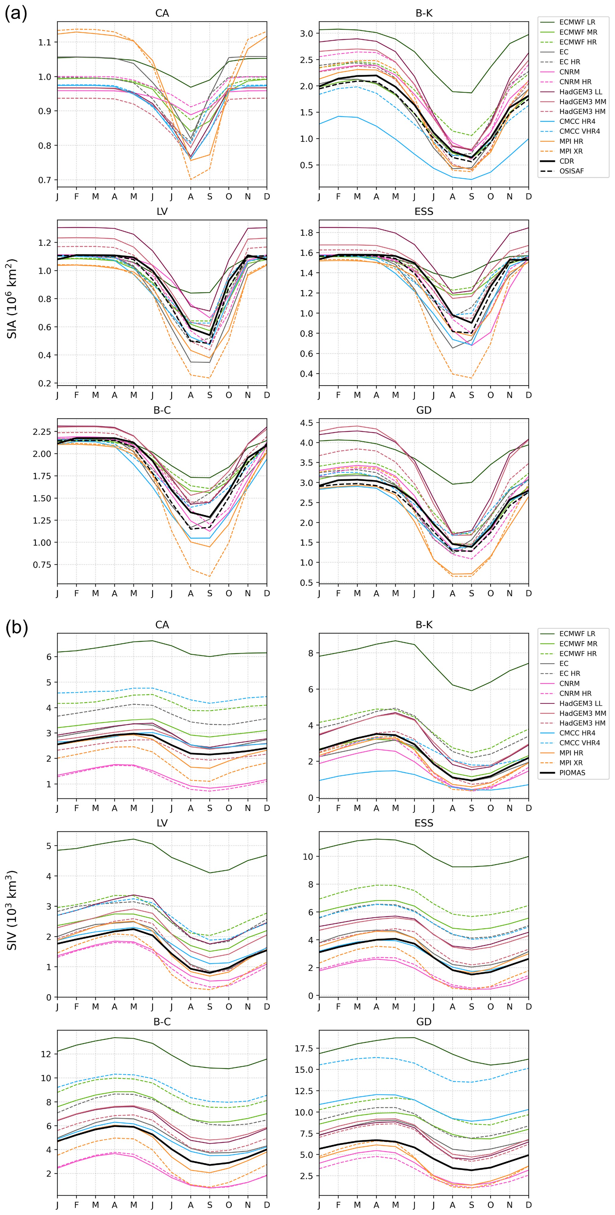
Figure 5 The 1979–2014 seasonal cycle in (a) SIA and (b) SIV in the Arctic sub-regions from HighResMIP hist-1950 model outputs versus CDR and OSI SAF for SIA and versus PIOMAS for SIV.

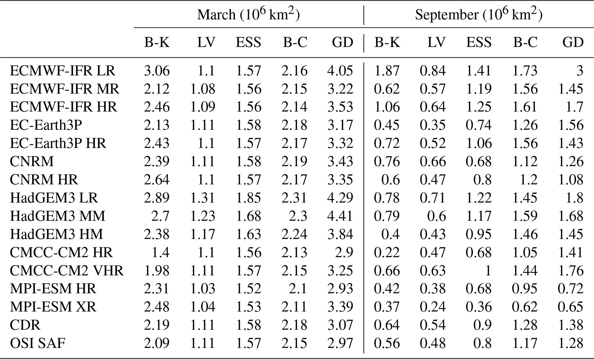
Table 2 March and September SIA for each region (except CA) in each model for 1979–2014.

Satellite estimates of SIA are not shown in the central Arctic sector (CA) due to the observation gap near the North Pole. In this region, all models simulate a pronounced seasonal cycle in SIA, with the widest area between December and April and a minimum in August. Although most models agree in winter when the region is fully covered by sea ice, the inter-model spread increases in summer. HadGEM3 and CMCC-CM2 simulate similar seasonal cycles in all configurations, with slightly lower values in HadGEM3 HM. The ECMWF-IFS LR is an outlier also in this region, with a large SIA all year round and a minimum in August that is as large as the autumn/winter values in other models. Also, EC-Earth3P LR has SIA comparable to ECMWF-IFS LR from November to May; however, it overestimates the melting and growing phases, with an August minimum comparable to other models. The CNRM-CM6 model produces the smallest seasonal cycle amplitude at both resolutions, with a decrease between the winter values and the minimum of ∼ 10 %. On the contrary, both MPI-ESM configurations display the strongest seasonal cycle, with the largest area in winter and the smallest in summer. These differences among models do not clearly depend on the resolution changes. For SIV, PIOMAS shows an increase of ∼ 30 % between the minimum in August/September and the maximum in May. The seasonal cycle magnitude is captured by most models, but with a large spread mainly driven by differences in the simulated thickness (Fig. 2). The models generally perform similarly in simulating the SIV seasonal cycle in the sub-regions and at the hemispheric scale (Fig. 3b). For the sake of conciseness, only the specific features of the SIV representation at the regional scale will be indicated below. The Barents–Kara seas (B-K) is the only sub-region where satellite products show a distinct maximum peak that occurs in April (1 month after the hemispheric SIA maximum); cf. Fig. 5a. Except for CMCC-CM2, the models generally overestimate SIA in winter, with a large spread among them which reduces in summer when models are in closer agreement with satellite estimates. The strong underestimation of SIA in the CMCC-CM2 HR4 configuration could be attributed to the increased poleward Atlantic OHT simulated by this model (Docquier et al., 2020). The warmer ocean temperatures not only promote sea ice melting in winter but also hinder its growth in autumn. The ocean and atmosphere spatial resolutions generally have the opposite effects on simulated SIA. Increasing only the ocean resolution in ECMWF-IFS (from LR to MR) and HadGEM3 (from LL to MM) results in lower SIA and a better fit to the observations. Conversely, increasing the atmosphere resolution generally leads to a larger SIA, except for a decrease in SIA in HadGEM3. The combined effect of enhanced resolution in both ocean and atmosphere in the CNRM-CM6 and EC-Earth3P models increases the winter SIA, exacerbating the disparity when compared to observational data. For SIV, nearly half of the model ensemble is within the 15 % of the PIOMAS seasonal variability from January to June, which is not the case for other sectors. The Barents–Kara seas is the only region where CMCC-CM2 HR underestimates SIV as a result of too low SIA. In addition, both configurations of CMCC-CM2 underestimate the seasonal variation in SIV. At the same time, CNRM-CM6 better fits PIOMAS SIV in the Barents–Kara sea sector compared to the other parts of the Arctic Ocean. The increased ocean resolution has a clear positive effect on SIV representation in ECMWF-IFS configurations, whereas other models display similar values when changing such parameter. On the other hand, the enhanced atmosphere resolution leads to higher SIV in ECMWF-IFS and CMCC-CM2, lower SIV in HadGEM3, and no affect on SIV in MPI-ESM.

The Laptev (LV), East Siberian (ESS), and Beaufort–Chukchi seas (B-C) show similar SIA and SIV behaviour. They can be analysed together and grouped as in Peng and Meier (2018). In these regions, there is no noticeable peak in the observed seasonal variability in SIA; instead, the annual maximum is extended between December and May since the winter sea ice expansion is constrained by land. In spring, the downward shortwave radiation increases, causing the rapid sea ice melt that ends in September. Notably, the disagreement between satellite estimates in summer SIA is higher in all three regions, probably due to the enhanced presence of melt ponds, which complicate the SIC retrievals from passive microwave radiometers (Ivanova et al., 2015). The models exhibit better agreement in winter, while the spread across models is larger in summer. This could possibly be associated with the model differences in simulating atmospheric circulation, river discharge (Park et al., 2020), and the transport of Pacific waters through the Bering Strait (Watts et al., 2021), which modifies the thermohaline structure of the upper ocean and affects sea ice growth and melt. In all three regions, SIA from ECMWF-IFS LR fits well with satellite estimates in winter, which is not the case for other sectors with a greater role of the Atlantic OHT where the model is biased high. HadGEM3 overestimates SIA, particularly in its lower-resolution configuration. This behaviour is also common for other parts of the Arctic Ocean, which points to the fact that bias in HadGEM3 is similarly distributed across the regions. MPI-ESM underestimates SIA to a greater degree in summer since the model is struggling to simulate consolidated pack ice (Fig. 2). CNRM-CM6, CMCC-CM2 and the HR run of EC-Earth3P show fairly good agreement with satellite estimates in all three regions. The lower-resolution configuration of EC-Earth3P displays an earlier and faster sea ice retreat in the Laptev and East Siberian seas, resulting in the second-lowest SIA, while the model compares well to OSI SAF estimates in the Beaufort–Chukchi seas. Increased ocean resolution leads to lower SIA for all models except for EC-Earth3P, which has higher values in its HR configuration. The effect of the ocean resolution is stronger in summer; however, the impact on HadGEM3 is substantial all year round. Enhancement of the atmosphere resolution does not significantly affect ECMWF-IFS but leads to higher summer SIA in CMCC-CM2 as well as in the other regions. For MPI-ESM, the increase in atmosphere resolution has a larger impact on summer SIA in the Laptev, East Siberian, and Beaufort–Chukchi seas compared to other sectors: MPI-ESM XR simulates SIA almost 2 times lower than CDR in August and September. In the Laptev, East Siberian, and Beaufort–Chukchi seas, SIV reaches a maximum in May (April–May in B-C), while the annual minimum occurs in September. Most models overestimate SIV, with the highest bias (ECMWF LR) in the East Siberian and Beaufort–Chukchi seas. CMCC-CM2 HR and MPI-ESM HR are the closest to PIOMAS, even though the latter fails to reasonably simulate SIC (Fig. 2). The effect of the ocean resolution on SIV is clearly seen in ECMWF-IFS and EC-Earth3P in all three regions and in HadGEM3 in the Laptev Sea – the only region where the LL and MM configurations of HadGEM3 differ. Other models do not show considerable differences in SIV when changing ocean resolutions. Finally, increased atmosphere resolution results in higher SIV for ECMWF-IFS, EC-Earth3P, and CMCC-CM2 and in lower SIV for HadGEM3 and MPI-ESM.

The Greenland region (GD) holds the largest area of sea ice in both winter and summer (3 and 1.5×10⁶ km², respectively, according to the satellite estimates). Most models tend to overestimate SIA all year round, with the highest bias in winter in ECMWF-IFS LR and HadGEM3. The models are generally capable of melting away the excess sea ice by August, so there is more consistency among most models in summer, when MPI-ESM underestimates SIA more than all other models. An increase in the ocean resolution from 1 to 0.25° effectively improves the representation of SIA in ECMWF-IFS, whereas it does not produce notable changes in HadGEM3 and EC-Earth3P. The effect of atmosphere resolution again depends on the model. ECMWF-IFS and CMCC-CM2 display slightly higher SIA in their finer-atmosphere configurations, particularly in winter. Conversely, HadGEM3 has lower SIA in its HM configuration in winter, which fits better to the observations. For MPI-ESM, there are no differences between different configurations, as can be seen in the Barents–Kara seas region. For SIV, both configurations of CMCC-CM2 have a large error in the Greenland region owing to high bias in SIT (Fig. 2), while at least one configuration of the model is in good agreement with PIOMAS in other sectors. Enhanced ocean resolution leads to lower SIV in ECMWF-IFS and higher SIV in EC-Earth3P. At the same time, there are no significant differences between configurations of HadGEM3 and CNRM-CM6 when changing ocean resolution. An increase in the atmosphere resolution has almost no effect on SIV in HadGEM3 and in MPI-ESM but leads to higher SIV in CMCC-CM2.

The displayed analysis reveals that the model performance and the accuracy of simulated SIA largely depend on the Arctic region and the season studied. While the Barents–Kara seas and Greenland regions mainly contribute to the winter inter-model spread, the largest summer differences among models are seen in the Laptev, East Siberian, and Beaufort–Chukchi seas. There are no considerable differences in the model abilities to simulate SIV at the regional scale; in fact, the biases are generally uniform across regions and seasons. Generally, we find no strong dependence of sea ice realism on the horizontal resolution. The impact of the ocean resolution on the representation of SIA is most pronounced in the Barents–Kara seas and Greenland sea ice regions that are strongly influenced by the Atlantic OHT. The effect of the atmosphere resolution is less clear, but there is evidence that the atmosphere resolution has a stronger impact on SIV rather than on SIA, particularly in the regions of thicker ice (B-C, GD).

3.4 Interannual variability and trends

Next, we evaluate the long-term variability in the Arctic SIA and SIV from the hist-1950 simulations from 1979 to 2014. Figure 6a illustrates monthly anomalies of SIA (with respect to 1979–2014 climatologies) simulated by the models and derived from satellite datasets. The inter-model spread is relatively similar throughout the period, but it increases from the mid-2000s when the ice reduction begins to accelerate. All models are able to reproduce the sea ice shrinking, but with varying intensities: ECMWF-IFS LR, HadGEM3 LL, and MPI-ESM HR show larger negative trends compared to observations ($-\mathrm{44}\times {\mathrm{10}}^{\mathrm{3}}$ km² yr⁻¹ in CDR and $-\mathrm{46}\times {\mathrm{10}}^{\mathrm{3}}$ km² yr⁻¹ in OSI SAF), while the MR and HR versions of ECMWF-IFS, both configurations of CNRM-CM6, EC-Earth3P, HadGEM3 HM, and CMCC-CM2 HR display weaker negative trends (Table 3). An increase in ocean resolution generally results in smaller negative trends, except for EC-Earth3P, which shows a similar decline rate in both configurations. Note that weaker trends are also observed in six HR ensemble members of ECMWF-IFR in comparison to their low-resolution counterparts (Table S1 in the Supplement). The effect of finer atmosphere resolution is different among models: the SIA decrease is stronger in ECMWF-IFS and CMCC-CM2 and weaker in HadGEM3 and MPI-ESM.

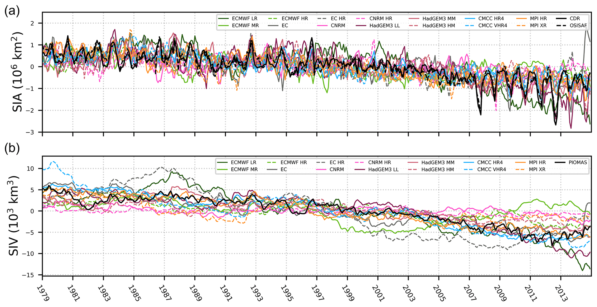
Figure 6 Monthly anomalies of SIA (a) and SIV (b) from 1979–2014 from HighResMIP model outputs and reference products.

Table 3 Linear trends in SIA and SIV and their standard deviations for the 1979–2014 and 2015–2050 periods.

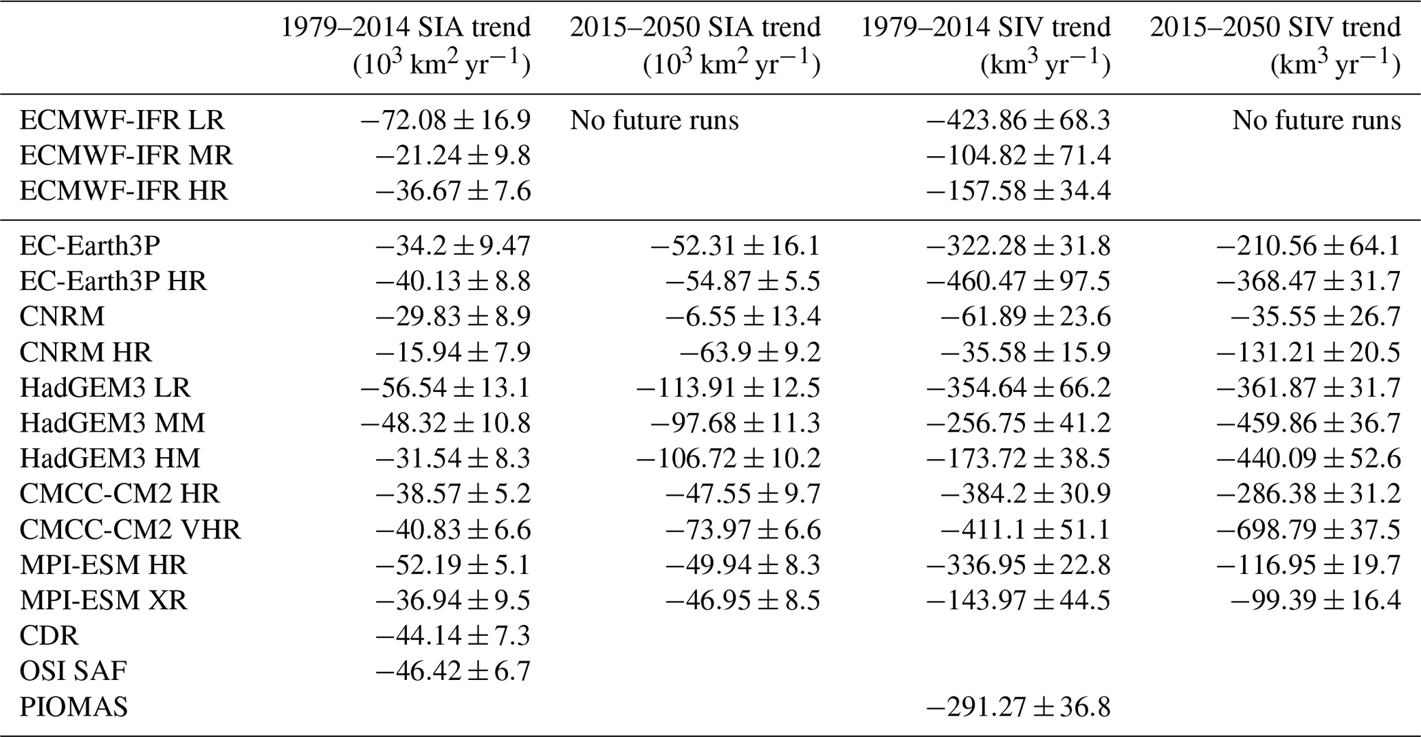
Figure 6b shows monthly anomalies of SIV (with the seasonal cycle removed) from 1979–2014 in the HighResMIP models and in PIOMAS. There is a substantial inter-model spread for SIV compared to SIA, particularly at the beginning and the end of the observed period (55 %–85 % of yearly averaged SIV from PIOMAS). The biases from a few models are not consistent throughout the years, varying significantly from positive to negative (EC Earth-3P HR, ECMWF MR, and HadGEM3 LL).

PIOMAS simulates sea ice shrinking at a rate of −291 km³ yr⁻¹; similarly, all models simulate a SIV decrease. There is no straightforward impact on the linear trends in SIV from changing resolution in the ocean and atmosphere since the impact of horizontal resolution on SIA and SIT differs between the models. However, we find that configurations with coarse ocean resolution generally tend to simulate more negative trends (−424 km³ yr⁻¹ in ECMWF LR compared to −105 and −157 km³ yr⁻¹ in its finer configurations; for HadGEM3, the trend ranges from −355 km³ yr⁻¹ at lower resolutions to −257 and −174 km³ yr⁻¹ in finer resolution configurations). We observe the same for the ECMWF ensemble members (Table S1). Here, the exception is EC-Earth3P, in which the eddy-permitting configuration has a larger negative trend in SIV (−322 and −460 km³ yr⁻¹). This might be attributed to the thicker ice simulated in the HR configuration (Fig. 2). In CNRM-CM6, the SIV decrease is very weak (−62 and −36 km³ yr⁻¹ for LR and HR configurations, respectively), which might reflect the negative ice growth–ice thickness feedback: thin ice allows sea ice to grow more rapidly, mitigating ice loss. The finer atmosphere resolution has a different impact on the pace of sea ice retreat in different models: CMCC-CM2, VHR4, and ECMWF-IFS HR simulate slightly stronger trends compared to their coarser counterparts (−384 and −411 km³ yr⁻¹ in CMCC-CM2 and −105 and −158 km³ yr⁻¹ in ECMWF-IFS). On the other hand, in MPI-ESM and HadGEM3, the finer configuration has less of a negative trend compared to the coarser one (−337 and −144 km³ yr⁻¹ in MPI-ESM and −174 and −257 km³ yr⁻¹ in HadGEM3).

We also examine how the models simulate sea ice response to external forcing on a seasonal scale. The monthly trends in the Arctic-wide SIA (computed over the period of 1979–2014) reveal that the models tend to underestimate the rate of sea ice loss in the melting season and in summer (not shown). Most models reproduce more negative trends from November to May and underestimate the magnitude of trends in other seasons. MPI-ESM HR trends are found to have a closer fit to the observed trends for the total Arctic, although the model simulates SIC and sea ice classes poorly. For SIV, the models vary greatly in the representation of trends. Despite all models being able to simulate a SIV decline in all months, they cannot capture the observed magnitude of sea ice loss and have values ranging from almost 0 to −450 km³ yr⁻¹. They also struggle to reproduce the seasonal cycle in the trends, which in PIOMAS has a slightly stronger signal in June and a weaker signal in the winter months (−320 and −260 km³ yr⁻¹, respectively).

Since there is a substantial difference in model performance in reproducing seasonal variability on a regional scale, we analyse monthly trends in SIA and SIV in each sea ice zone from 1979–2014 (Fig. 7). The magnitude and timing of sea ice loss strongly depend on the season and region. According to observations, the winter decrease in SIA is most dramatic in the Barents–Kara seas (nearly $-\mathrm{17}\times {\mathrm{10}}^{\mathrm{3}}$ km² yr⁻¹; 0.8 % yr⁻¹), while the summer trends are dominated by the Eastern Siberian Sea and Beaufort–Chukchi seas (almost $-\mathrm{25}\times {\mathrm{10}}^{\mathrm{3}}$ km² yr⁻¹; 2 %–3 % yr⁻¹). The Barents–Kara seas and the Greenland region show a pattern of SIA trends that differs from the total Arctic and the rest of the regions, which have one pronounced negative peak in September and trends close to zero in winter. Instead, in the Atlantic sector, i.e. the Barents–Kara seas and Greenland coast, sea ice loss is observed all year round with a slightly stronger decrease in July. In the central Arctic, the models simulate a weak SIA reduction, with the strongest signal in August–September, which is not significant in most models (less than 5 % of the SIA of the sector). In the other sectors, the models generally tend to underestimate the pace of sea ice loss indicated by satellite estimates. The exception is the Barents–Kara seas and the Greenland sector, where some models produce more negative trends compared to the observations. In the Laptev, East Siberian, and Beaufort–Chukchi seas, some of the models do not simulate a reduction in summer SIA and even display weak yet insignificant positive trends. Given that all these regions contain a large MIZF in summer (Fig. 4), the inability to capture trends points to inaccurate sensitivity of sea ice to external forcing, particularly within the MIZ.

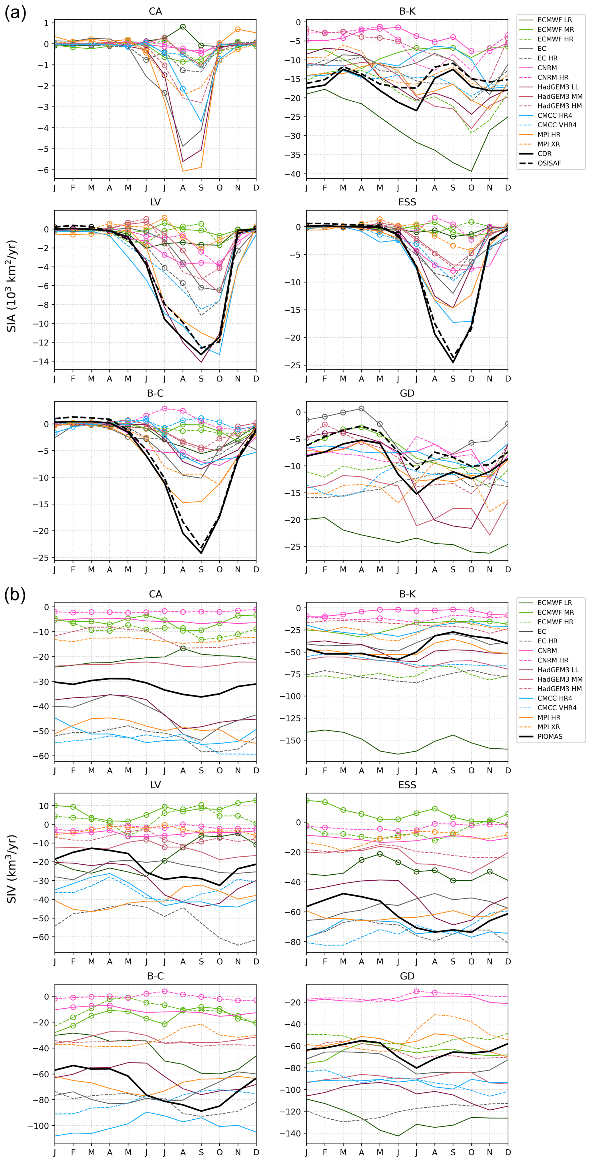
Figure 7 The 1979–2014 monthly trends in SIA (a) and SIV (b) in the Arctic sub-regions for HighResMIP hist-1950 model outputs versus CDR and OSI SAF for SIA and versus PIOMAS for SIV. Dots indicate non-significant trends.

The strongest negative trends in SIV are observed in the areas of thick ice: the Beaufort–Chukchi seas (up to −90 km³ yr⁻¹ in September), the Greenland sector (−80 km³ yr⁻¹ in July), and the East Siberian Sea (−70 km³ yr⁻¹ in summer months). The seasonal cycle of the Barents–Kara sea SIV trend contrasts with that of other sectors, where the highest rate of sea ice decline is observed in September. Notably, in the Laptev, East Siberian, and Beaufort–Chukchi seas, SIV experiences a substantial decrease in the winter months, while SIA stays nearly stable, reflecting a considerable ice thinning primarily driven by basal melting. In the East Siberian Sea and Beaufort–Chukchi seas, almost all models tend to underestimate trends in SIV (10 out of 14 model simulations produce less-negative trends), while in the rest of the Arctic zones, PIOMAS is nearly in the middle of the inter-model spread. Compared to other models, both CNRM-CM6 configurations and the two finest configurations of ECMWF-IFS have changes in SIA and SIV closest to zero in almost all regions and months. On the one hand, CNRM-CM6 simulates very thin ice, so the lack of trend is consistent with the concept of negative ice thickness–ice growth feedback. On the other hand, ECMWF-IFS MR and HR underestimate sea ice reduction everywhere despite simulating very thick ice. HadGEM3 performs differently at the regional scale, but at least one of the configurations has a very good fit to the PIOMAS estimates. Generally, both configurations of CMCC-CM2 present the large SIV decrease in all sectors except for the Barents–Kara Sea, and the rate of decline is similar between the two resolutions despite a significant difference in the mean SIV. The HR configuration of MPI-ESM is in fairly good agreement with PIOMAS in all regions except the central Arctic and the Laptev Sea, where it tends to produce more negative trends. Conversely, MPI-ESM XR underestimates negative SIV trends in all parts of the Arctic Ocean, except the Greenland zone where it is close to its HR configuration.

Overall, there is no consistent link between the strength of sea ice retreat and the ocean/atmosphere resolution: it instead depends on the region and the model used. Considering only SIA, the models generally underestimate the trends, especially in finer ocean configurations and in the Laptev, East Siberian, and Beaufort–Chukchi seas in summer. However, the beneficial effects of increased ocean resolution for SIA trends are observed for ECMWF-IFS in the Barents–Kara seas and in the Greenland area. In these regions, other models do not differ considerably between configurations: low- and high-resolution configurations show a closer fit to the observations according to the season. Moreover, the increased atmosphere resolution also does not improve the representation of SIA trends: the HadGEM3, CMCC-CM2, and MPI-ESM finer atmosphere configurations lead to underestimating the negative SIA trends more than their counterparts at coarse resolutions do. The relation between ocean/atmosphere resolution and SIV trends is less clear and depends on the region and the model.

3.5 Future projections

In this section, we analyse the results of HighResMIP models when simulating future Arctic sea ice changes, using highres-future model outputs from 2015 up to 2050. HighResMIP future projections generally show stronger sea ice loss compared to historical runs (Table 3). These simulations can elucidate when the Arctic will reach its first ice-free summer, i.e. the condition typically defined as the timing when September sea ice drops below 10⁶ km². Reaching ice-free conditions is an unprecedented change in the Arctic environment and the tipping-point in the Earth's climate system. Considering the large inter-model spread in simulating observed mean sea ice state and trends, we assume that a selection of the models which better agree with observations can reduce the spread and decrease uncertainty in the model projections. We select models based on the historical performance of September SIA and SIV mean state and trends versus CDR and PIOMAS, respectively (Fig. 8). To exclude outliers, we define the 75th-percentile threshold, and we select the models whose values do not exceed the threshold for both variables. The resulting subset includes four models: the low-resolution configuration of EC-Earth3P, HadGEM3 MM and HM, and CMCC-CM2 HR. These models are used in the further analysis of sea ice future evolution.

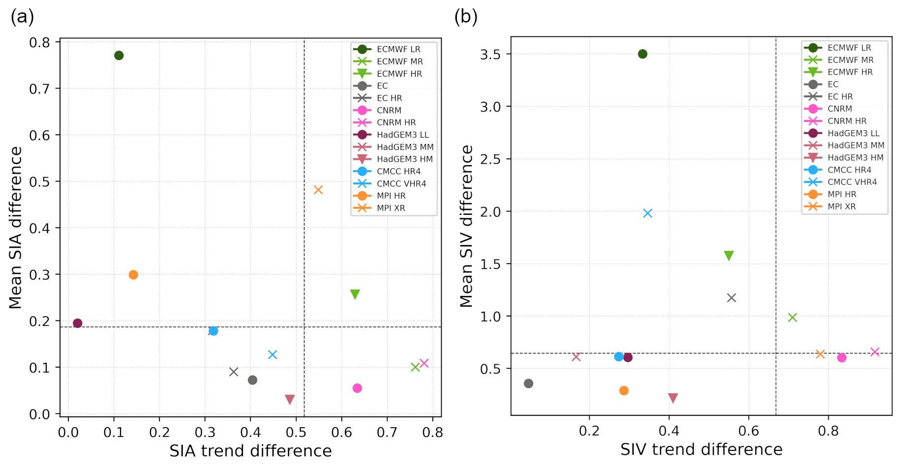
Figure 8 Normalized difference in the mean September SIA versus September SIA trend from 1979–2014 (a). Same for SIV (b). The difference is computed with reference to CDR (for SIA) and PIOMAS (for SIV). Dashed lines indicate the 75th percentile for a set of the model outputs excluding ECMWF-IFS.

Figure 9 illustrates the September SIV time series from 1950 to 2050 computed for the total Arctic and for the sub-regions. The vertical lines mark the first ice-free September in the multi-model mean with and without model selection (yellow and green, respectively) and in CDR (black, data available between 1971–2021). At the regional scale, the timing of ice-free conditions refers to the threshold of 25 % of the CDR SIA averaged over the 1980–2010 period in the given region. It is evident that a huge sea ice reduction takes place in all Arctic sectors; however, the pace of sea ice loss varies across the regions owing to differences in the initial state and dominant processes driving the change. We note that applying model selection results in earlier timing of the ice-free conditions in Barents–Kara, Laptev, East Siberian, and Beaufort–Chukchi seas and in ice-free conditions in the total Arctic, central Arctic, and Greenland region. In the latter sub-regions, the multi-model mean without model selection does not predict the event everywhere before 2050. The comparison between the model configurations in simulating the timing of ice-free conditions shows that there is no clear link between the model resolution and the pace of sea ice loss (not shown).

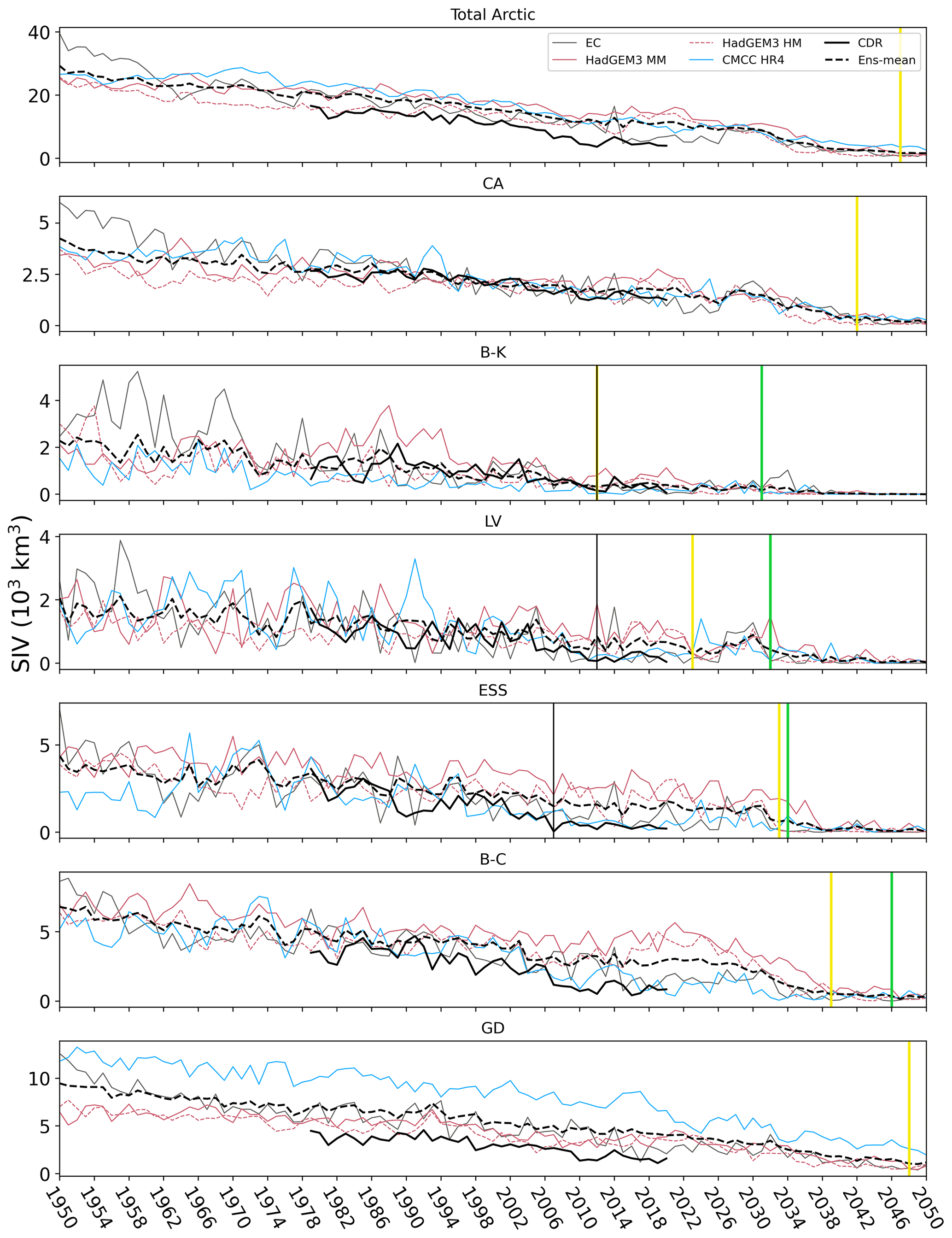
Figure 9 Time series of September SIV from 1950 to 2050 using HighResMIP historical and future runs and PIOMAS for the entire Arctic and sub-regions. The multi-model mean SIV with model selection is shown by the dashed line. The vertical lines indicate the year of ice-free conditions: green for the multi-model mean without model selection, yellow for the multi-model mean with model selection, and black for CDR. “Ice-free conditions ”signifies that SIA falls below 10⁶ km² for the total Arctic and reaches 25 % of the CDR SIA averaged over 1980–2010 for the sub-regions.

The September Arctic-wide sea ice from the multi-model mean (with model selection) shrinks by 95 % from 1950 to 2050; cf. the top panel of Fig. 9. The inter-model spread decreases throughout the century, from 14×10³ in 1950 to 1.64×10³ km³ in 2050. The Arctic does not reach ice-free conditions before 2050 in the multi-model mean without model selection, although applying selection criteria advances the timing of the event to 2047. The central Arctic September sea ice will lose 96 % of its volume by 2050 in the multi-model ensemble, which is in good agreement with PIOMAS during the overlapping period. The inter-model spread again narrows substantially, from 2.58×10³ km³ in 1950 to 0.23×10³ km³ in 2050. Ice-free conditions in the central Arctic are not reached before 2050 in the multi-model mean when considering all models. However, the exclusion of outliers leads to approaching the threshold in 2042. The Barents–Kara seas experience the most dramatic sea ice loss, accounting for almost 100 % of SIV from 1950 to 2050 in the model ensemble. The first ice-free September in the Barents–Kara seas is accurately simulated by the multi-model mean with model selection: the event occurs in 2012, as shown in CDR. Avoiding model selection postpones the event by 19 years. In the Barents–Kara seas, the spread among models decreases from 1.46×10³ km³ in 1950 to almost vanishing in 2050. The multi-model mean SIV in the Laptev Sea shrinks by 99 % in 100 years. The inter-model spread narrows from nearly 0.9×10³ km³ at the beginning of the run to 0.05×10³ km³ at the end. The timing of the first ice-free summer is similar to that in the Barents–Kara seas: SIA drops below the threshold in 2012 in CDR and in 2032 in the multi-model mean without model selection. When applying selection criteria, ice-free conditions are reached in 2023. In the East Siberian Sea, September ensemble-mean SIV is reduced by 99 % by the middle of this century. The East Siberian Sea reaches the threshold in SIA earlier compared to the other regions. CDR produces the event in 2007, when the Arctic broke the first record low, while the multi-model mean with model selection simulates the first ice-free conditions in 2033 (2034 without model selection). The inter-model spread ranges between 4.76×10³ km³ in 1950 and 0.1×10³ km³ in 2050. The Beaufort–Chukchi seas lose nearly 96 % of SIV in 100 years in the ensemble mean. The inter-model spread decreases from 3.44×10³ km³ at the beginning to 0.37×10³ km³ at the end of the run. The multi-model mean reaches the first ice-free September in 2046. When adopting model selection, the Beaufort–Chukchi seas will be ice-free in 2039. The Greenland region is undergoing the least prominent sea ice loss, accounting for 88 % throughout the period from 1950 to 2050. However, there is a great narrowing of the inter-model spread from 6.12×10³ km³ in the middle of the last century to 1.15×10³ km³ 100 years after. Both multi-model means project that Greenland SIA might turn ice-free in 2048. Overall, the models simulate the first ice-free September later than CDR in all sub-regions studied. Therefore, we can reasonably assume the same behaviour for the total Arctic.

Along with overall sea ice loss, there are substantial changes in the structure of sea ice cover. Figure 10 shows the time series of September SIA and the MIZF from 1950 to 2050. For SIA (top panel), the models are in fairly good agreement with the observations yet have systematic biases and underestimate the negative trend. In addition, the inter-model spread is large but relatively similar throughout the years (∼ 4×10⁶ km²). For the MIZF (bottom panel), the spread among models increases considerably with time, from ∼ 10 % in 1950 to ∼ 75 % in 2050. Most models simulate MIZF growth, which reflects the transition of the sea ice state to the marginal, ice-dominated state. MIZ in the 2040s is projected to account for up to 80 % of the total ice area in September, although the interannual variability at the end of the run is large in most models. The CNRM-CM6 and MPI-ESM models are two outliers: CNRM-CM6 has a nearly constant MIZ fraction during the whole period, while MPI-ESM has MIZF close to 100 % from the beginning of the run, but it occasionally drops to 0 at the end of the run. Distinct model performances in simulating MIZF show that an accurate representation of total SIA does not guarantee the same for all sea ice classes, highlighting the importance of studying the Arctic MIZ.

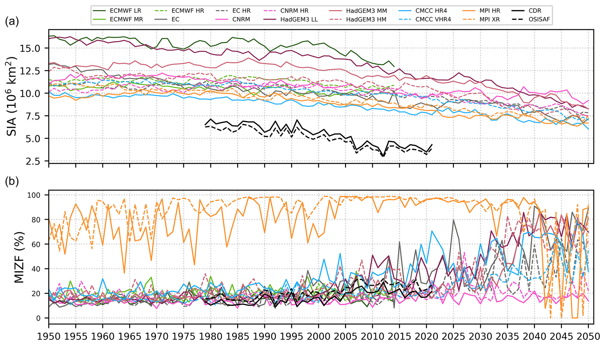
Figure 10 Time series of September SIA (a) and MIZF (b) from 1950 to 2050 using HighResMIP historical and future runs and satellite products (CDR and OSI SAF).

4 Discussion

Although the latest generation of the models does a fairly reasonable job simulating the mean state and long-term variability in sea ice cover (Notz and Community, 2020), the models still suffer from biases, which decrease model trustworthiness in projecting the future sea ice state in the Arctic. The enhancement in the model component horizontal resolutions is used in CMIP6 HighResMIP as one of the factors capable of improving the realism of the model simulations and reducing biases in polar regions. In this study, we investigated the ability of HighResMIP to simulate Arctic sea ice variability and the impact of the ocean and atmosphere horizontal resolution on the representation of sea ice properties in the recent-past and future climate. We do not find a strong link between ocean/atmosphere resolution and the representation of sea ice properties, and the realism of model performance instead depends on the model used. Nevertheless, there is evidence that enhanced ocean resolution leads to an improved representation of winter SIA in some models. This is associated with more accurate meridional heat transport (Docquier et al., 2019), which is a key process that can regulate the location of the ice edge and of SIA (Li et al., 2017; Muilwijk et al., 2019). The Atlantic Ocean is the main heat source entering the Arctic, accounting for 73 TW on average per year (Smedsrud et al., 2010); therefore, an adequate simulation of the boundary currents is particularly important in the Atlantic sector of the Arctic Ocean, which is confirmed by the regional analysis in our study. Another process that might be sensitive to horizontal ocean resolution is the Arctic river discharge, which contributes to both seasonal variations in sea ice cover and long-term sea ice variability. The freshwater input stabilizes the upper ocean stratification and isolates the warm Atlantic layer from the bottom of the sea ice cover (Carmack et al., 2015), resulting in higher ice growth in winter. On the other hand, the heat input from the rivers accelerates sea ice melt and increases the ocean temperature, which has possible implications for the next year's growing season (Park et al., 2020). Representation of river discharge in HighResMIP models needs additional investigation. Our results do not show a systematic impact of atmosphere resolution on the representation of the Arctic sea ice. This is confirmed by other studies reporting the minor role of atmosphere resolution compared to that of the ocean (Roberts et al., 2020; Koenigk et al., 2021; Meccia et al., 2021). However, increasing atmosphere resolution might permit a more realistic representation of precipitation, which can lead to increased snowfall (Strandberg and Lind, 2021) and consequently generate cooling and sea ice expansion (Bintanja et al., 2018).

SIT is less responsive to changes in the ocean grid resolution compared to SIA, and its representation largely depends on the sea ice model. Our results show that in some cases large biases in SIT reduce the beneficial effect of increased horizontal resolution on SIA. Poor representation of SIT is a great obstacle to the robustness of sea ice projections. The high uncertainty cannot be overcome without constraining the model simulations with a sufficient number of in situ measurements of the Arctic SIT, which are still sparse and unreliable (Massonnet et al., 2018). Apart from the horizontal resolution, there are other important factors affecting the model performance, for example inaccurate representations of mixed layer depth (Watts et al., 2021), surface air temperature (Papalexiou et al., 2020), surface pressure and geostrophic winds (Kwok and Untersteiner, 2011; Stroeve et al., 2014), and sea ice sensitivity to global warming (Zhang, 2010). These elements pair with the intrinsic complexity of sea ice models that include thermodynamics schemes and parameterizations (Keen et al., 2021), sea ice dynamics components (Hunke, 2010), and coupling between the ocean and atmosphere components (Hunke et al., 2020). Given that there were few improvements with increased horizontal resolution, we argue that running the models at higher resolutions might not be worth the major effort of costly computations. Our results suggest that the efforts of the modelling groups should be aimed rather at the improvement of the sea ice model physics and parameterizations.

Our analysis is limited to only one ensemble member of each model configuration, which does not allow for a proper assessment of the role of internal variability. It is important to emphasize that internal variability can easily lead to marked differences between the basic features of the climate models. Results from large ensembles of multi-decadal simulations are required to robustly quantify internal climate variability and convincingly identify deficiencies and demonstrate the potential progress of the climate models (e.g. Deser et al., 2020; Maher et al., 2020). Large ensembles with individual CMIP-class models show that the differences between ensemble members reflect simulated internal variability. For Arctic sea ice, internal variability has a large influence on multi-decadal trends (e.g. Swart et al., 2015) and has reinforced anthropogenic September Arctic ice loss since 1979 (Kay et al., 2011). Using a single member or small ensembles to conclude that a climate model is in error can lead to inappropriate conclusions about the model fidelity. While a large number of ensemble members is desirable to account for fluctuations due to internal variability, we acknowledge that these are computationally expensive and may not always be available. Unfortunately, not all HighResMIP models used in this study provide multiple members. ECMWF-IFR LR, MR, and HR have 8, 3, and 6 ensemble members, respectively, and EC-Earth3P and CNRM have 3 ensemble members for both the LR and HR systems. Only one member is available for all the other configurations. In the Supplement, we provide additional analysis of the abovementioned models that includes all existing model members to show the weakness and robustness of the single-model response. For these three models, we show SIA and SIV variability on seasonal (Figs. S1, S3, and S5 in the Supplement) and interannual (Figs. S2, S4, and S6 in the Supplement) timescales and linear SIA and SIV trends (Tables S1–S3 in the Supplement) from 1979 to 2014 for ensemble members with LR and HR configurations. The minimum and maximum deviation among the “control” member for each month depict the bounds of simulated internal variability. The internal variability tends to be largest in late autumn and winters and smallest at the summer sea ice minimum when the reduced ice coverage leads to relatively low variability, as seen in the seasonal cycle. In this case, the effect of resolution does not depend on the choice of ensemble member. The magnitude of the 36-year trends in SIA and SIV is most affected, but the small-ensemble mean is generally comparable with the single-member results (with the exception of the CNRM ice area). Still, the LR area and volume exhibit stronger (weaker) negative trends than their HR counterparts in ECMWF (EC-Earth3P). It is worth noting that these very small ensembles do not offer considerably better sampling of internal climate variability than a single-model ensemble. Although the correct sampling of internal variability is a necessary condition for assessing model fidelity, it is also crucial to assess how the model simulates the physical mechanisms of interest. However, our analysis highlights the fact that large ensembles of multi-decadal credible simulations, along with strengthening of the effort towards developing more realistic climate models, are needed to understand sea ice trends.

In this study, we try to understand when the Arctic will see its first ice-free summer using HighResMIP outputs. Models show a wide temporal range for the occurrence of ice-free conditions in the Arctic. To reduce the inter-model spread in sea ice projections, we apply a widely used approach based on the selection of models according to their historical performance (Wang and Overland, 2012; Senftleben et al., 2020). Although close agreement with observations does not guarantee the realism of the models, we believe that excluding the models that struggle to reproduce the present-day SIA and SIV mean state and trends might improve the accuracy of future sea ice projections. Different criteria to select “best-performing” models exist and almost always lead to earlier near-disappearance of sea ice compared to no selection (Docquier and Koenigk, 2021). The timing of the first ice-free Arctic in our model selection compares well with similar criteria applied to CMIP6 models that predict the event between 2047 and 2052, while the process-based criteria advance the timing of the first ice-free summer to 2035 (Docquier and Koenigk, 2021). However, the investigation of model selection criteria is outside of scope of this study; our goal is to give insight into when the Arctic might turn ice-free.

Our results highlight the increasing role of the MIZ in the response of Arctic sea ice to climate change. We show that the MIZ will be the dominant sea ice class in the Arctic by 2050, which implies a shift to new sea ice conditions similar to those in Antarctica. The chaotic interannual variability in the summer MIZF in the last years of simulations indicates that current model physics might not be suitable for changing sea ice conditions (Fig. 10). In order to realistically simulate (thermo)dynamical processes, the new sea ice regime requires modifications in model physics and sea ice rheology, which is formulated for thick pack ice (Aksenov et al., 2017). Additionally, the growing fraction of the MIZ requires changes in the parameterization of the lateral and basal melt (Smith et al., 2022). The proper simulation of the MIZ is essential for achieving reasonable projections of future sea ice conditions since small and thin ice floes within the MIZ are more vulnerable to external dynamic and thermodynamic forces than consolidated pack ice is. In addition, the water patches between the ice floes permit the absorption of solar radiation in the upper ocean, increasing the role of the ice–albedo effect, which causes anticipation of the ice advance onset and acceleration of the overall sea ice loss. To demonstrate positive feedback between summer MIZ and minimum SIA for the following year, we plot the mean MIZF over June, July, August, and September (JJAS) versus September SIA with a 1 year lag, computed for the years 2015–2050 (Fig. 11a). All models except one simulate negative regressions ranging from ∼ −0.13 % per 10⁶ km² to −0.06 % per 10⁶ km², which means that the larger summer MIZF leads to lower September SIA the following year. We suggest that the MIZ might act as a predictor of future sea ice conditions in the model simulations. Figure 12b shows JJAS MIZF in 2015 (start of the highres-future run) versus the first September when the Arctic becomes ice-free. Note that not all models simulate the event before 2050. Our analysis indicates that with higher initial MIZF, the September sea ice disappears earlier. This indicates that a reasonable representation of the MIZ at the beginning of the run might impact the pace of sea ice loss and potentially improve the accuracy of model projections. We assume that the MIZF might represent a robust criterion to examine model fidelity. The impact of the MIZ on the accuracy of the model simulations needs further investigation.

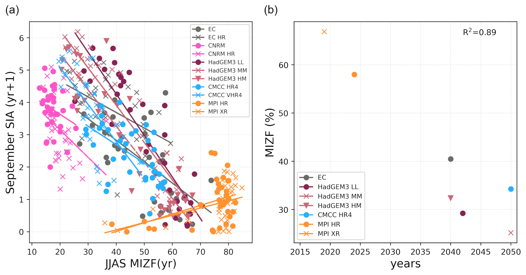
Figure 11 June, July, August, and September (JJAS) MIZF mean versus September SIA with a 1-year lag, from 2015–2050 (a). Timing of the first ice-free Arctic year versus JJAS MIZF in 2015 (b).

5 Conclusions

In this study, we evaluate the historical and future variability in the Arctic sea ice area and volume using six coupled atmosphere–ocean general models participating in the HighResMIP experiments of the sixth phase of the Coupled Model Intercomparison Project (CMIP6). For the period of 1979–2014, we find that most models can properly simulate the maximum and minimum of the SIA seasonal cycle at hemispheric and regional scales. However, some of them cannot correctly capture their magnitude, failing to realistically reproduce the ice growth and retreat phases, with systematic overestimation or underestimation of the seasonal variability. We find that the models are generally able to reproduce the seasonal cycle of the Arctic-wide MIZ area, although not all of them can capture the timing of the annual maximum. The models simulate different areas of the MIZ, especially in summer; however, there is stronger agreement among models regarding MIZF. We find that different regional contributions to the inter-model spread are associated with seasonal variability: the winter inter-model spread in SIA is attributed to the Atlantic sector (Barents–Kara seas and the Greenland ice zones), while the summer differences are tied to the Laptev, East Siberian, and Beaufort–Chukchi seas.

Selected models differ broadly across the spatial distribution of the mean SIT and its average values. Only a few models reveal a pattern similar to PIOMAS, characterized by thicker ice off the coast of Greenland and the Canadian Arctic Archipelago. Most models simulate ice that is too thick, which affects the representation of sea ice volume; excluding one outlier, all but two models overestimate ice volume all year round: up to 1.5 times in April and 3.5 times in August. However, regardless of large systematic biases, most models simulate a realistic seasonal cycle of SIV with a maximum in April and a minimum in August. All models capture declines in SIA and SIV over the historical period, but they disagree on the pace of sea ice loss. The response to the external forcing does change with season and region: the winter trends are dominated by changes in the Barents–Kara seas and the Greenland ice zone, while the summer trends are driven by those in the East Siberian and Beaufort–Chukchi seas. Most models underestimate ice loss in all regions, particularly in summer; conversely, they tend to simulate more negative trends in the Greenland zone, leading to overestimating the Arctic-wide SIA trend in some configurations. In this study, we find that there is no strong relationship between ocean/atmosphere resolution and sea ice cover representation: the impact of horizontal resolution rather depends on the studied variable and the model used. However, the ocean has a stronger effect than the atmosphere and an increase in ocean resolution from ∼ 1 to ∼ 0.25° has a favourable impact on the representation of SIA and sea ice edges, which is especially evident for the ECMWF-IFS and HadGEM3 models. At the same time, the simulation of SIT does not directly rely on the grid spacing or on the derived SIV. A finer ocean resolution leads to lower SIV for ECMWF-IFS and to almost no differences for HadGEM3. On the other hand, enhanced atmosphere resolution leads to higher SIV for ECMWF-IFS and CMCC-CM2, and increasing the resolution in both the ocean and the atmosphere results in little difference between configurations in CNRM and in higher SIV for EC-Earth3P. We also find that the differences between configurations vary from one region to another, which highlights the importance of examining the model performance at a regional scale. For example, SIA and SIV are too low in CMCC-CM2 HR4 in the Barents Sea, caused by overestimating the OHT at the Barents Sea Opening (Docquier et al., 2020), while performing well in the rest of the sectors. On the other hand, MPI-ESM has similar SIA in two configurations in the Barents–Kara seas and the Greenland ice zone, whereas the finer-atmosphere configuration displays less sea ice in summer in the rest of the regions.

Considering the period 2015–2050, all models simulate a long-term decrease in SIA and SIV, with a generally stronger rate of ice loss compared to the historical period. Model simulations predict that the Arctic loses nearly 95 % of SIV from 1950 to 2050. There is again no systematic impact of horizontal resolution on the occurrence of the first ice-free conditions. The multi-model mean of all models does not project the Arctic to become ice-free before 2050. However, applying model selection based on historical performance advances the event to 2047. Considering that the model selection leads to closer agreement with CDR on the year of the first ice-free summer in the regions where it has already happened (the East Siberian, Barents–Kara, and the Laptev seas), we infer that model selection application may potentially improve the accuracy of model projections of Arctic sea ice evolution. Together with overall ice shrinking, we studied the changes in the structure of sea ice cover, and we concluded that the MIZ will constitute up to 60 %–80 % of the September SIA by 2050. This suggests a shift to a new sea ice regime similar to that in the Antarctic. Given that the MIZ will play a major role in the response of the Arctic sea ice to external forcing, modifications in the model physics and parameterizations are encouraged in the new generations of coupled climate models.