the Creative Commons Attribution 4.0 License.
the Creative Commons Attribution 4.0 License.
 | 12 Jan 2024
Modeled variations in the inherent optical properties of summer Arctic ice and their effects on the radiation budget: a case based on ice cores from 2008 to 2016
Peng Lu
Matti Leppäranta
Bin Cheng
Ruibo Lei
Bingrui Li
Qingkai Wang
Zhijun Li
Variations in Arctic sea ice are apparent not only in its extent and thickness but also in its internal properties under global warming. The microstructure of summer Arctic sea ice changes due to varying external forces, ice age, and extended melting seasons, which affect its optical properties. Sea ice cores sampled in the Pacific sector of the Arctic obtained by the Chinese National Arctic Research Expedition (CHINARE) during the summers of 2008 to 2016 were used to estimate the variations in the microstructures and inherent optical properties (IOPs) of ice and determine the radiation budget of sea ice based on a radiative transfer model. The variations in the volume fraction of gas bubbles (Va) of the ice top layer were not significant, and the Va of the ice interior layer was significant. Compared with 2008, the mean Va of interior ice in 2016 decreased by 9.1 %. Meanwhile, the volume fraction of brine pockets increased clearly during 2008–2016. The changing microstructure resulted in the scattering coefficient of the interior ice decreasing by 38.4 % from 2008 to 2016, while no clear variations can be seen in the scattering coefficient of the ice top layer. These estimated ice IOPs fell within the range of other observations. Furthermore, we found that variations in interior ice were significantly related to the interannual changes in ice ages. At the Arctic basin scale, the changing IOPs of interior ice greatly changed the amount of solar radiation transmitted to the upper ocean even when a constant ice thickness is assumed, especially for thin ice in marginal zones, implying the presence of different sea ice bottom melt processes. These findings revealed the important role of the changing microstructure and IOPs of ice in affecting the radiation transfer of Arctic sea ice.
- Article
(2943 KB) - Full-text XML
-
Supplement
(461 KB) - BibTeX
- EndNote


The recent rise in air temperature in the Arctic is almost twice the global average, known as Arctic amplification (Dai et al., 2019), which has been seen in the retreat of sea ice, especially in summer. The extent of sea ice in summer has decreased (Comiso et al., 2008; Parkinson and Comiso, 2013; Petty et al., 2018), and summer ice is thinner (Kwok, 2018), younger (Stroeve and Notz, 2018), and warmer (Wang et al., 2020) than before. These changes have affected the transfer of sunlight into the Arctic Ocean, and the optical properties of sea ice are changing the solar radiation budget in the area.
Variations in Arctic sea ice cover are related not only to the macroscale properties described above but also to the ice microstructure. Sea ice is a multiphase medium consisting of pure ice, gas bubbles, brine pockets, salt crystals, and sediments (Hunke et al., 2011). In the last few decades, the length of the Arctic ice melt season has shown a significant positive trend (Markus et al., 2009), and the Arctic ice cover has experienced a transition from predominantly old ice to primarily first-year ice (Tschudi et al., 2020; Stroeve and Notz, 2018). At the same time, in melting ice, gas bubbles and brine pockets tend to become larger (Light et al., 2003), and phase changes due to brine drainage and temperature result in variations in the volume of gas and brine (Crabeck et al., 2019; Weeks and Ackley, 1986). Except for the abovementioned factors, absorption of shortwave radiation, synoptic weather, and surface melt pooling can also partly affect the ice microstructure. Therefore, the physical properties of ice have changed, and in the past 10 years the bulk density of summer Arctic sea ice has been lower than reported in the 1990s due to increased ice porosity (Wang et al., 2020). Despite the changing ice microstructure having attracted attention, there is still no quantitative description of its evolution and affecting factors (Petrich and Eicken, 2010).
Gas bubbles and brine pockets, as dominant optical scatterers, directly influence the inherent optical properties (IOPs) of sea ice (Grenfell, 1991; Perovich, 2003a). IOPs include scattering and absorption coefficients and information about the phase function of the domain. The varying IOPs of ice have attracted attention due to their important role in the process of light penetration in ice. Light et al. (2008) and Katlein et al. (2019, 2021) demonstrated clear different IOPs in sea ice of different depths. The differences in the IOPs between first-year ice and multiyear ice have been ascertained in many observations (e.g., Light et al., 2015; Grenfell et al., 2006). There are also some differences in the bulk IOPs of first-year ice because of the different stages of melting (Veyssière et al., 2022). However, the available observed or estimated ice IOPs were rare, which resulted in quantitative knowledge of the progression of the sea ice IOPs and their influencing factors still being absent (Light et al., 2015). Even in the latest studies and sea ice models, IOPs are set as constants based on previous field observations (Briegleb and Light, 2007), which is somewhat in contrast to the reality in the Arctic Ocean.
Changes in ice microstructure or IOPs are especially important for the energy budget of Arctic ice under the general warming climate and decreasing ice age. The reason for this is their direct effect on ice apparent optical properties (AOPs), which influence the partitioning of radiation in the Arctic by various feedback processes. However, the observed relationships between ice microstructure, IOPs, and AOPs are rare in the available literature. Parameterization proposed by Grenfell (1991) has been the most widely used method to estimate the response of ice IOPs to microstructure. Due to the lack of detailed, observed ice microstructure, this method has usually been used to build models (Light et al., 2004; Yu et al., 2022; Hamre, 2004). In the latest MOSAiC expedition during 2019–2020, Smith et al. (2022) observed the formation of a porous surface layer (i.e., surface scattering layer, SSL) of sea ice and its enhancement of ice albedo. Macfarlane et al. (2023) described the microstructure of the SSL in further detail using X-ray tomography and its effects on ice optical properties. The authors are the first to link ice microstructure and optical properties by field observations.
In this study, in situ observations of the physical properties of summer Arctic sea ice during the Chinese National Arctic Research Expedition (CHINARE) from 2008 to 2016 were employed as input data. Variations in the microstructure and the IOPs of Arctic sea ice are presented. Also shown are their quantitative effects on the radiation budget. Applying these varying IOPs to satellite-observed sea ice conditions has allowed us to estimate the role of ice microstructure in the radiation budget on the Arctic basin scale.
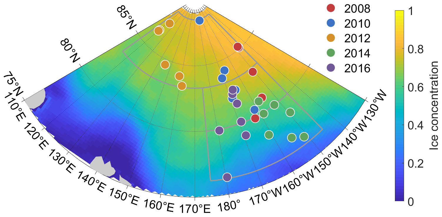
Figure 1Locations of the sampled ice cores during CHINARE cruises. The ice cores were sorted into three parts according to latitude and ice concentration. Their quantities were nearly the same in each zone. The ice concentration in the base map is the mean in August from 2008 to 2016.
2.1 Arctic sea ice coring
The Arctic sea ice cores were sampled in the Pacific sector of the Arctic Ocean during summer cruises of the CHINARE program from 2008 to 2016 (Fig. 1). The ice cores in each year were composed of different quantities of first-year ice and multiyear ice with thicknesses from 0.6 to 1.9 m. Detailed volume fractions of the gas bubbles and brine pockets (Va, Vb) in the ice cores were given by Wang et al. (2020). The mean sampling date of ice cores was 20 August ±8 d, when the ice had been melting for a while (∼59 d) and had not yet begun to freeze according to the melting onset data from NASA. According to previous observations, the SSL of sea ice can be re-formed within a couple of days of removal (Smith et al., 2022). There are no clear temporal changes in the microstructure of surface ice in the whole of July (Macfarlane et al., 2023). Furthermore, the ice surface melt rate in August was only of that in July (Nicolaus et al., 2021; Perovich, 2003b). That is, it is expected that the microstructure of the ice surface was similar in the middle and late melting seasons that cover the sampling dates of the present ice cores. Therefore, the short-term temporal variability in ice cores was expected not to affect their surface ice microstructure.
To further reduce the impact of temporal variations in the ice cores on the ice microstructure, we preprocessed the ice core data. The ice cores in each year were allocated different weights according to their sampling date. The weight (w) of ice cores in the affecting period (D) can be obtained according to the Cressman method: , where d is the number of days from the mean sampling date. Then the weighted mean of ice properties was . D was set to 30 d because the weighted mean values and deviations were nearly unaffected when D was over 30 d. In the following analyses, the mean values of each year refer to the weighted ones. After the preprocessing, the deviation of melting days in a single year was reduced by ∼50.5 %. As for the spatial variations in the ice cores, it is difficult for field observations to avoid the effects of spatial variations. Therefore, related studies have generally ignored the effects of sampling locations on the statistics (Carnat et al., 2013; Frantz et al., 2019; Katlein et al., 2019; Light et al., 2022). Related discussion about the temporal and spatial variations can be found in Sect. 4.2.
A typical undeformed sea ice floe consists texturally of three layers due to its growth conditions (Tucker et al., 1992). The first two layers are relatively thin and consist of a granular layer and a transition layer, and the lowest layer generally consists of columnar ice. The ice texture controls the ice microstructure (Crabeck et al., 2016). Thus, the development of gas bubbles, brine pockets, and IOPs in the three ice layers is different. Analogously to the parameterization of the Los Alamos sea ice model (CICE; Briegleb and Light, 2007), Each ice core was evenly divided into 10 layers. The top () layer of an ice core was defined as the top layer (TL), the second layer () was the drained layer (DL), and layers – collectively constituted the internal layer (IL). Note that the surface scattering layer (SSL) and part of the DL were mixed in the TL and could not be separated completely. Layer was also a mixture of the DL and IL and is therefore neglected in the following analysis.
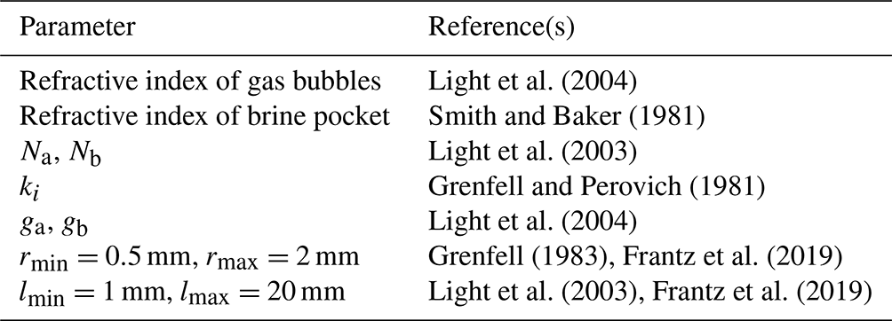
Table 1Parameters used in the radiation transfer model in the Arctic summer and their sources.
2.2 Sea ice optics modeling
The IOPs of sea ice, including the scattering coefficient, σ; absorption coefficient, κ; and asymmetry parameter, g, can be determined directly from the ice microstructure. Following the theory of Grenfell (1991), scattering in ice is caused by gas bubbles and brine pockets and absorption is caused by brine pockets and pure ice. This parameterization has been proved by extensive observations (Light et al., 2004; Smedley et al., 2020). The IOPs of sea ice can be obtained from the sum of the scatterers weighted by their relative volumes as
In these equations, the subscripts a and b represent gas bubbles and brine pockets, respectively, and r is their radius (or equivalent radius) and l the length of the brine pockets. Qsca and Qabs are the scattering and absorption efficiencies, respectively, which can be calculated using Mie theory. N is the size distribution function. Subscript i represents pure ice, and is its volume fraction. The values of these parameters are summarized in Table 1. Brine pockets longer than 0.03 mm are modeled as cylinders rather than spheres (Light et al., 2003). The conversion function from Grenfell and Warren (1999) is employed to represent hexagon columns as spheres with the same optical properties. Besides, Qabs and Qsca in the required size range are obtained using their effective radii, which are calculated according to Hansen and Travis (1974).
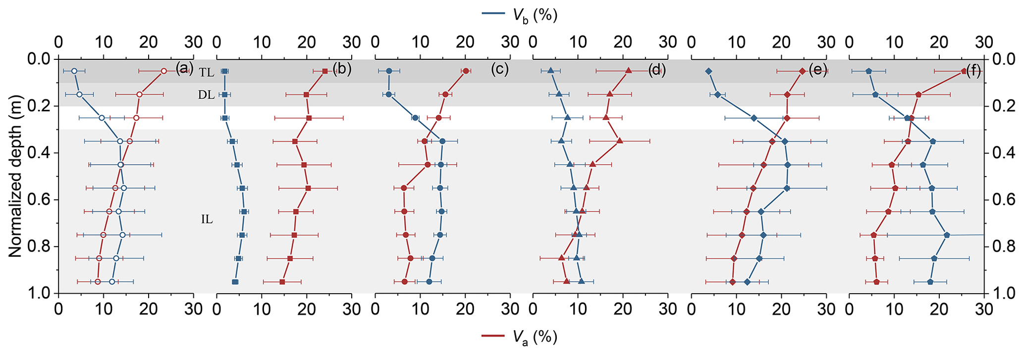
Figure 2Profiles of Va and Vb against normalized depth in (a) the whole study period, (b) 2008, (c) 2010, (d) 2012, (e) 2014, and (f) 2016. The error bars show the standard deviation from the mean of the results. The shaded areas represent the ice layer structure.
The delta-Eddington multiple-scattering model, where the constant IOPs from Briegleb and Light (2007) were replaced by the modeled IOPs, was employed to estimate the apparent optical properties (AOPs: albedo αλ, transmittance Tλ, and absorptivity Aλ) of the ice at the sampling sites (Yu et al., 2022). This radiative transfer model has been commonly used, and its accuracies have been widely accepted. The integrated albedo (αB), transmittance (TB), and absorptivity (AB) were calculated by integrating the spectral values over the band of the incident solar radiation, F0, as
In the following sections, the integrated absorption coefficient, κB, was also derived by this equation, following CICE (Briegleb and Light, 2007). Considering the generally cloudy weather in Arctic summer, the incident solar irradiance under an overcast sky in August from Grenfell and Perovich (2008) was chosen as the default value for F0. The studied wavelength band was set as the photosynthetically active band: λ1=400 nm and λ2=700 nm.
2.3 Arctic-wide up-scaling
To conduct an up-scaling analysis of the radiative budget of the Arctic sea ice cover based on observations of the ice microstructure in the Pacific sector, we used representative basin-scale sea ice data to estimate the variations in the distribution of radiation fluxes in summer during 2008–2016. The sea ice concentration (C) was provided by the National Snow and Ice Data Center (NSIDC) (DiGirolamo et al., 2022), the sea ice thickness was based on CryoSat-2/SMOS data fusion (Ricker et al., 2017), and the downward shortwave radiation flux at the surface (Ed) was obtained from the European Centre for Medium-Range Weather Forecasts (ECMWF). The latter two data sets were interpolated to a 25 km NSIDC polar stereographic grid. Then, the mean radiation fluxes and ice concentrations from July to September from 2008 to 2016 were set as the representative values in summer. Due to the limitation of satellite remote-sensing data of summer ice thickness, the representative thickness was estimated according to the mean value in October from 2011 to 2016, together with the growth rate estimated by Kwok and Cunningham (2016). Then, representative ice thickness can be obtained. These gridded ice thickness and IOP profiles from ice cores were inputted into the radiative transfer model to estimate the ice AOPs. From all these data sets and the derived parameters, the reflected, absorbed, and transmitted radiation fluxes by Arctic sea ice were calculated as , , and , respectively.
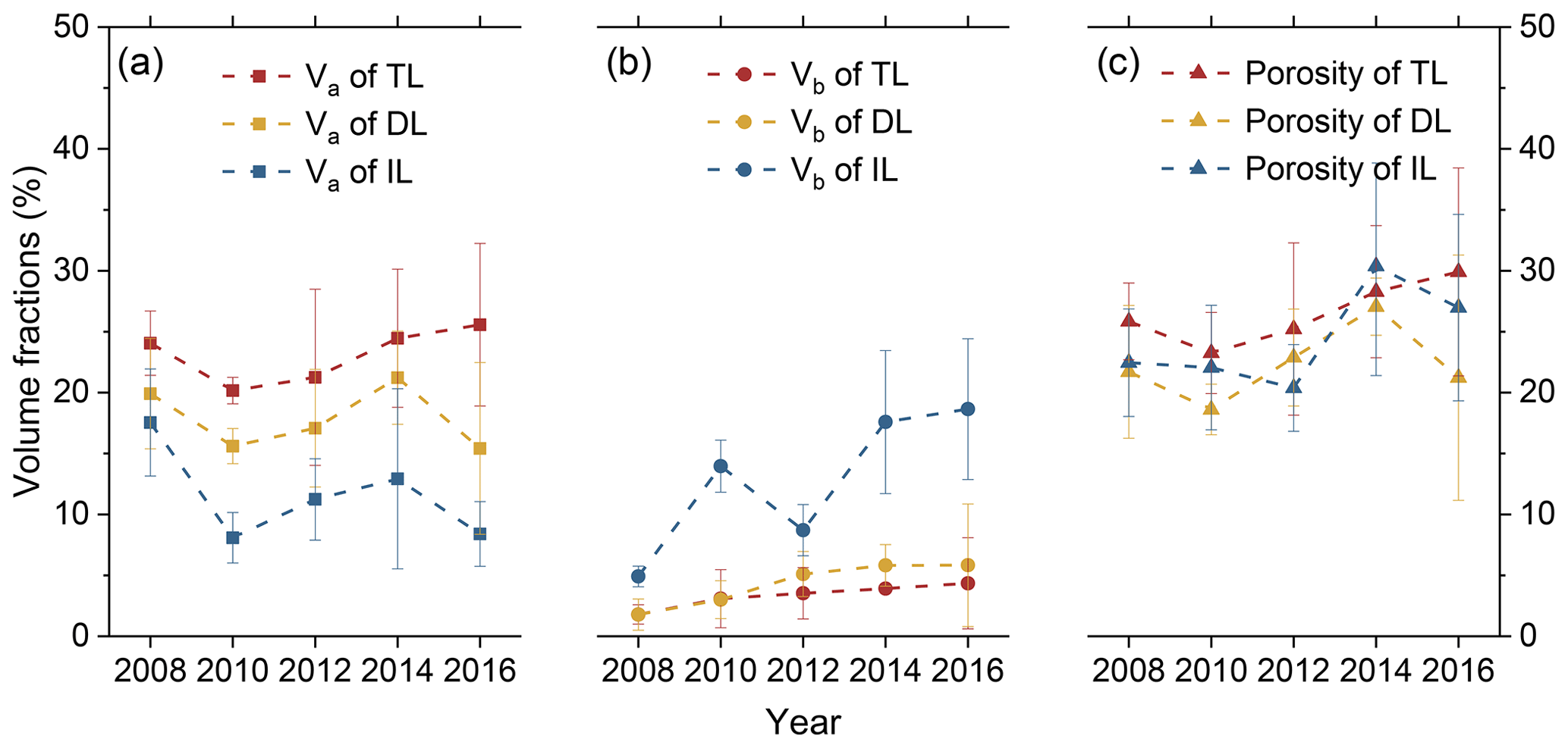
Figure 3Variations in (a) Va, (b) Vb, and (c) the porosity of the TL, DL, and IL of the ice cores during 2008–2016. The error bars show the standard deviation for each year.
3.1 Microstructure of the ice cores
There were different variation trends in the volume fraction of gas bubbles and brine pockets (Va, Vb) as a function of ice core depth (Fig. 2). The upper granular ice was typically bubbly, associated with the drainage of brine, and the interior columnar ice was usually depleted in gas bubbles (Cole et al., 2004). Thus, a significantly different Va could be seen (analysis of variance (ANOVA), P<0.01) with a decreasing trend along depth (Pearson correlation coefficient , P<0.01). The mean Va of the TL, DL, and IL for all ice cores was 23.4 ± 5.6 %, 17.9 ± 5.3 %, and 11.6 ± 5.9 %, respectively. These values are similar to the observations made by Eicken et al. (1995), where Va decreased from >20 % at the top to <5 % at the bottom for summer Arctic sea ice.
The different Vb values between layers were significant (ANOVA, P<0.01). The drainage of brine resulted in a relatively small Vb of TL, with a mean of 3.5 ± 2.4 %, while it was 4.6 ± 3.1 % and 13.5 ± 6.7 % in the other two layers, respectively (Fig. 2a). Vb=5 % is usually chosen as a threshold where discrete brine inclusions start to connect and the columnar ice is permeable enough to enable drainage (Carnat et al., 2013). Thus, the ice cores in the present study have been melting for some time, agreeing with the sampling season during CHINARE. Most Vb profiles had a maximum in the middle depth, except for the ice cores in 2012 (Fig. 2d). This can be explained by the later sampling date in 2012 relative to the other years by about 10 d, which resulted in enhanced brine drainage. Furthermore, the shape of the Vb profile was also associated with the ice age (Notz and Worster, 2009). Compared with the ice cores in 2010, although the ice cores in 2016 had similar sampling dates (1 d difference), the maximum position of Vb in 2016 was lower than in 2010 (Fig. 2c, f). This was because all ice cores in 2010 were sampled from first-year ice, and the ice cores in 2016 were comprised of first-year ice and multiyear ice (Wang et al., 2020).
In addition to the different variations in Va and Vb with depth, the annual variations in each layer were also different (Fig. 3a). Va was relatively small in the TL of 2010 because all ice cores were sampled from first-year ice (Wang et al., 2020). The quantities of first-year ice cores were similar to the quantities of multiyear ice cores in the other years. The variation in Va of the TL between years was statistically insignificant (ANOVA, P>0.1). This indicated that the melting process of the ice surfaces of the cores in different years was not different significantly. Contrary to the TL, the Va in the IL was different significantly (ANOVA, P<0.05). Compared with 2008, the mean Va of the IL in 2016 decreased by 9.1 %. The Va values of the DL were relatively stable and did not show significant variations in the study period.
Things were different for Vb and ice porosity. There were increases in the mean Vb of all three ice layers (Fig. 3b). Furthermore, the increases in mean Vb in the IL were statistically significant (r=0.84, P<0.1; ANOVA, P<0.01). From 2008 to 2016, the increase in the mean Vb of the IL was 13 %. Simultaneously, the ice salinity of the IL decreased (Fig. S1 in the Supplement), which agreed well with the observed and modeled results with warming conditions (Vancoppenolle et al., 2009). From the combined effects of changing Va and Vb, there are no significant differences in the porosity of three layers (ANOVA, P>0.1). Furthermore, the developments of porosity in the three layers are also similar (Fig. 3c). Among the three layers, the statistical significance of changing porosity of the IL between years was relatively good (ANOVA, P<0.1).
3.2 Variations in the IOPs of the ice cores
The mean scattering coefficient, σ, of the TL, DL, and IL for all ice cores was 264.5 ± 26.7, 208.9 ± 26.5, and 160.9 ± 33.3 m−1, respectively (Fig. 4a). There was a significant decreasing tendency along with depth in the mean σ of all ice cores (, P<0.01; ANOVA, P<0.01), associated with a decreasing volume of gas bubbles (Fig. 2). Although the Vb values of the ice cores increased clearly with depth, their effects on ice σ were covered by the decreasing Va. The reason for this was that the refractive indices of brine pockets and pure ice are close (Smith and Baker, 1981; Grenfell and Perovich, 1981), which results in the effects of brine pockets on ice σ being relatively weak compared to the gas bubbles.
The vertical variations in κB and g were not clear unlike for σ because they depend on Vi and , respectively. Due to the effects of the ice porosity (Va+Vb), κB did not show a statistically significant trend with depth (ANOVA, P>0.1), which varied in the range 0.09–0.1 m−1. The mean value of g was 0.93 except in 2008 (which was g=0.89), and it significantly increased with depth (r=0.91, P<0.01; ANOVA, P<0.01). This value is similar to the commonly used one; for example, the previous typical range of g was from 0.86 to 0.99 (Ehn et al., 2008), and 0.94 was often adopted for computational efficiency in models (Light et al., 2008). We note that the volume of brine pockets in ice cores of 2008 is relatively small, which was a reason for the different values of g found here.
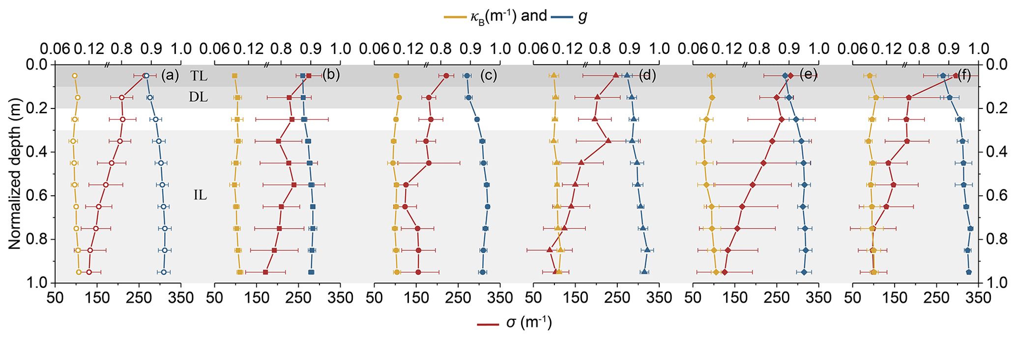
Figure 4IOP profiles of ice cores against normalized depth in (a) the whole study period, (b) 2008, (c) 2010, (d) 2012, (e) 2014, and (f) 2016. The error bars show the standard deviation from the mean of the results.
The annual mean IOPs of the TL, DL, and IL of the ice cores are shown in Fig. 5. As shown in Fig. 5a, the variations in σ of the TL, DL, and IL were different. The variation in σ of the TL between years was statistically insignificant (ANOVA, P>0.1), which reveals the relatively stable scattering ability of the ice surface. Things were different for the IL: there were statistically significant variations in σ between years (ANOVA, P<0.05). Compared with 2008, the σ of the IL in 2016 decreased by 38.4 % due to the decreased Va (Fig. 3). The overall variations in the σ of the DL were similar to those seen in the IL, whereas the former variations were not as clear as the latter due to ongoing drainage and were not significant (ANOVA, P>0.1).
There were no statistically significant differences in the integrated absorption coefficient, κB, of the TL, DL, and IL (ANOVA, P>0.1), indicating that the absorptivity of ice in different depths is similar. Furthermore, the developments of κB in the three layers are similar (∼0.001 yr−1, Fig. 5b). Among the three layers, the statistical significance of changing κB values of the IL between years was better (ANOVA, P<0.05) than of the TL and DL. As shown in Fig. 5c, the values of g of the TL and DL were nearly constant. Because their values of Vb were sufficiently small and similar due to drainage (Fig. 3b), their values of g are mainly attributed to gas bubbles. In contrast, the g of the IL varied significantly (ANOVA, P<0.01). The values of g of the IL increased by 5 % with increasing Vb in the study years (Fig. 3b).
3.3 Variations in the AOPs of the ice cores
Having seen that the IOP profiles of the sea ice were not constant in the different years (Fig. 5), a more important question is how these changes affected the AOPs. The radiative transfer model was employed here to estimate the AOPs of sampling sites, as shown in Fig. 6. Note that the AOPs here were calculated based on the level ice. Surface properties, such as a snow layer or melt ponds, were not considered here because the focus was on the effects of the ice microstructure on ice AOPs. The results obtained with the same IOP profiles but for a constant reference ice thickness (1 m) are also presented to quantify the contributions from the ice microstructure and thickness separately. This reference thickness was chosen to study the vertical structure relation to the surface and bottom and compare the samples with different thicknesses. This does not affect the trends in Fig. 6.
It can be seen from Fig. 6a that the thickness of ice cores decreased in study years with a statistically significant trend (, P<0.05) and variations (ANOVA, P<0.05). The values of αB changed because of the effects of the ice IOPs and thickness (Fig. 6b). The variations in mean αB during 2008–2014 were similar to those in the σ of the TL and DL. In 2016, the mean αB decreased due to the decreasing ice thickness. As a result, there are no statistically significant variations in αB between years (ANOVA, P>0.1). This was different from the remote-sensing results (−0.05 per decade from 1982 to 2009) of Lei et al. (2016). Part of the reason for this was that the direct factor that reduces the annual ice albedo is not the ice microstructure but rather the surface conditions. Eicken et al. (2004) and Landy et al. (2015) reported that the evolution of melt ponds on the ice surface could explain 85 % of the variance in the summer ice albedo.
Differently from αB, annual variations in TB and AB were significant (ANOVA, P<0.05). The TB (AB) tended to increase (decrease) with years (Fig. 6c). The mean value of TB in 2016 was over treble that in 2008. Meanwhile, AB decreased by about 19.5 % from 2008 to 2016. Furthermore, the change in AB in the study years was lower than the actual change in the ice thickness (−35.0 %). Thus, the difference, 23.8 % , was attributed to an increase in the absorbed solar energy per unit volume of sea ice. This result does match the findings of Light et al. (2015), which showed that the thickness of first-year ice was less by 13.3 % than multiyear ice (1.3 m vs. 1.5 m, respectively). However, the radiation absorbed by the former was less by 2 % than the latter. In other words, the solar energy absorbed by a unit volume of first-year ice was greater than multiyear ice by 12.5 %.
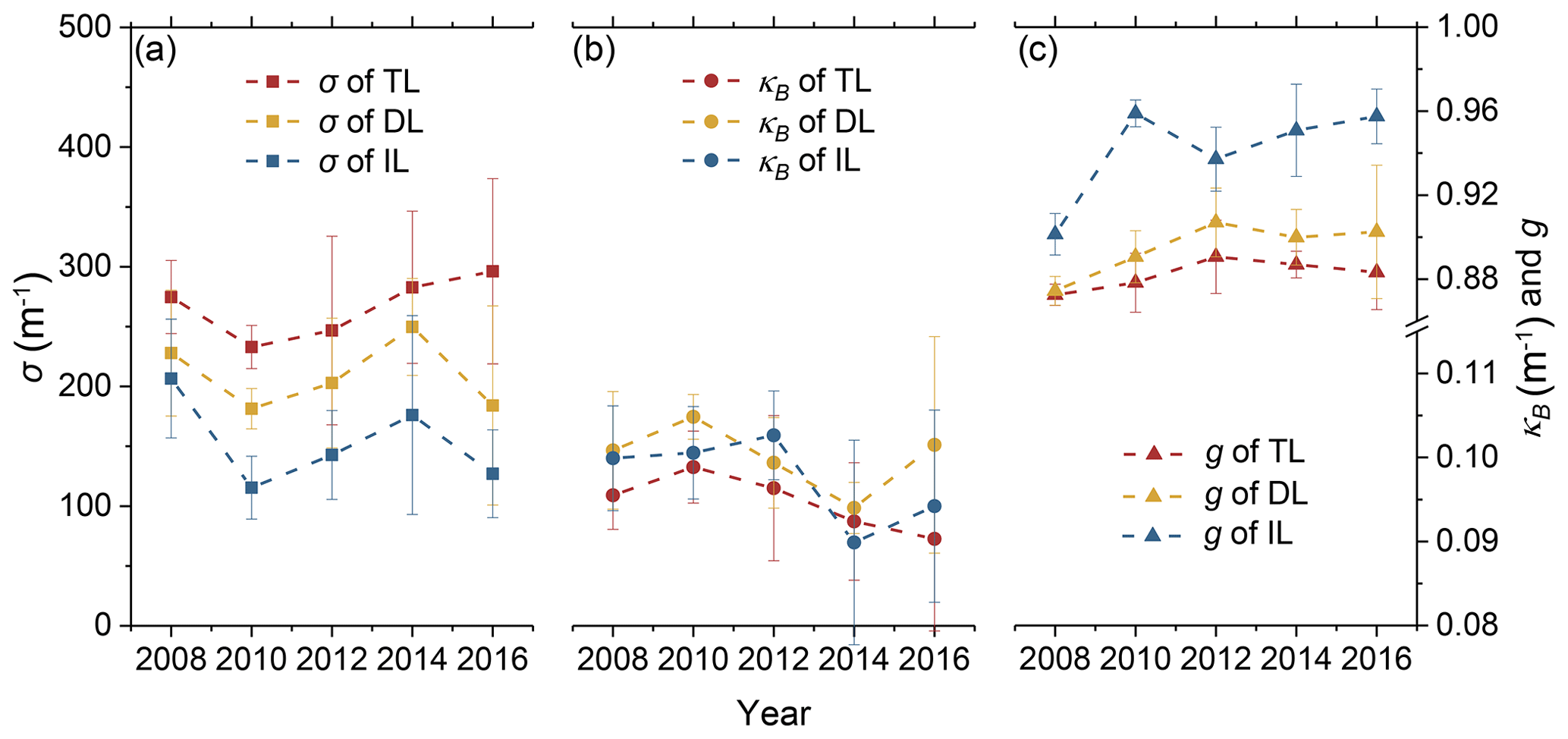
Figure 5Annual (a) σ, (b) κB, and (c) g for the TL, DL, and IL of the ice cores from 2008 to 2016. The error bars show the standard deviation in each year.
To make a direct comparison with the above variations, we considered a constant ice thickness, finding no clear changes in αB (Fig. 6b). Meanwhile, the variations in TB and AB were clearly different with similar overall trends (dashed lines in Fig. 6c). TB increased from 0.03 to 0.07 from 2008 to 2016, accounting for about 33.1 % of the real change ratio with changing thickness. Thus, the changing microstructure of the melting ice resulted in an increased transmittance that was independent of the ice thickness. A similar result was observed in the laboratory, where the changing ice microstructure during the warming process (no decrease in thickness) increased the ice transmittance (Light et al., 2004). Differently from TB and AB, whether the thickness was accounted for or not, the variations in αB were hardly affected. This demonstrated that the present variations in ice thickness had more effects on the ice TB and AB than αB.
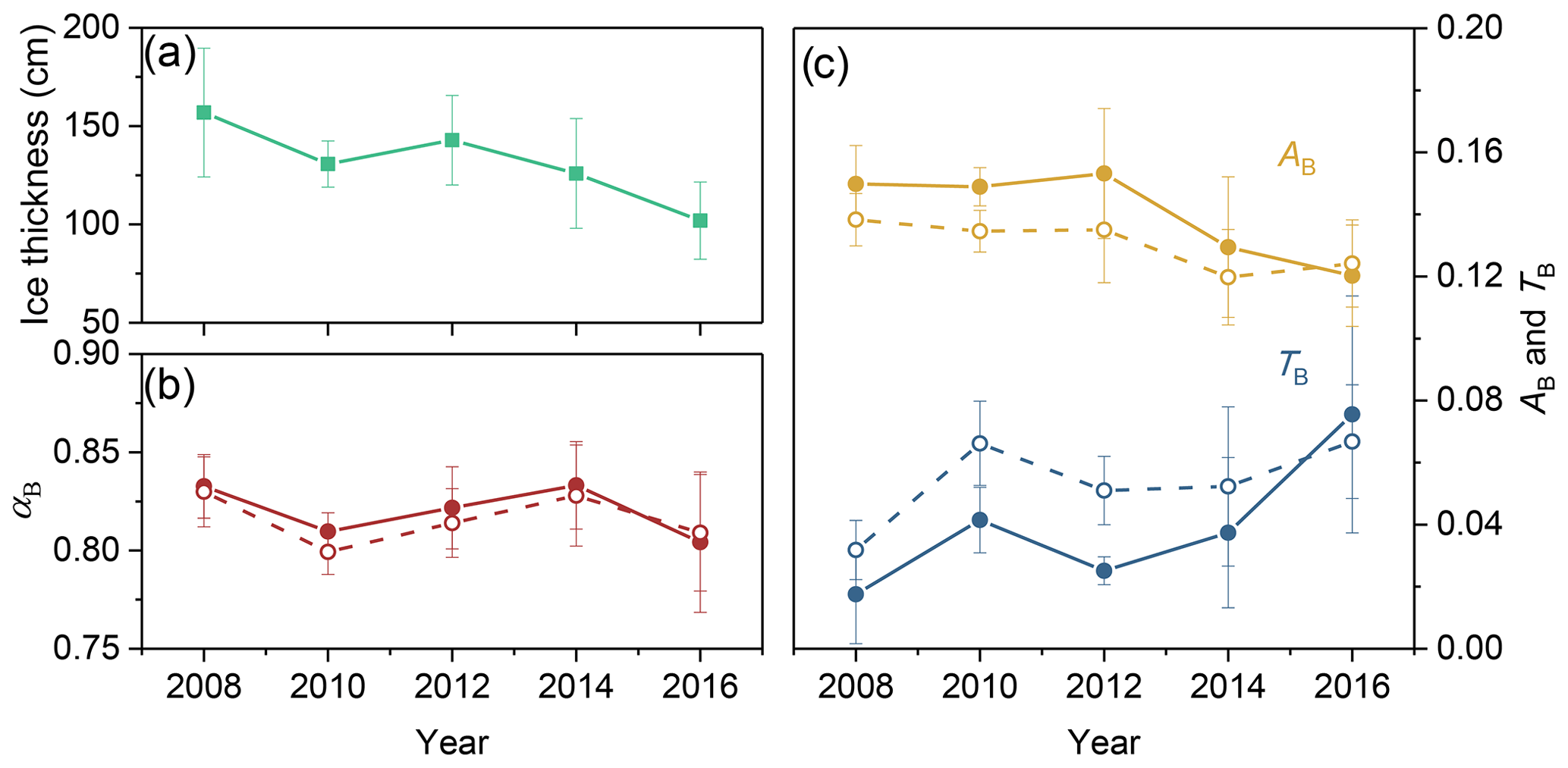
Figure 6(a) Thickness and (b, c) estimated AOPs of the ice cores from 2008 to 2016. Also shown as dashed lines are the AOPs with the same IOPs and constant thickness (1 m). The error bars show the standard deviation in each year.
3.4 Arctic-wide estimation
It may be interesting to estimate the quantitative effects of varying IOPs on the radiation distribution of the Arctic with a real ice thickness field. We expand the variations in the ice cores (Fig. 5) to an Arctic-wide scale under the following assumptions. (1) The IOPs of Arctic ice can be represented by our ice cores data. They are taken as constant, and seasonal and spatial differences are ignored. This is justified since such a hypothesis has been widely used (Briegleb and Light, 2007). (2) A decreasing trend of −5.8 cm yr−1 in ice thickness according to Lindsay and Schweiger (2015) was adopted to obtain a general view of the contributions of the changing ice thickness to the radiation budget. The representative basin-scale sea ice and radiation data in summer (see Sect. 2.3) were used here to estimate the variations in the distribution of radiation fluxes.
With the combined effects of the changing microstructure and thickness of ice, Arctic-wide variations in the mean αB, TB, and AB were statistically significant (ANOVA, P<0.01) and clearer than those in Fig. 6 (Fig. 7a), especially the overall trends of the mean TB (r=0.95, P<0.01) and AB (, P<0.01) of ice. Although the mean αB decreased from 2008 to 2016, there was not much change in reflected solar flux (Er), about 51.2 W m−2 during the study years (Fig. 7b). This resulted from the decreasing αB being largely provided by marginal ice zones. The decreasing rate of αB in regions with ice thicknesses <1 m (equivalent to 16.4 % of the entire ice area) was over 1.6 times the rate of the entire ice cover (Fig. S2). With the retreat of sea ice, the reflected flux of the marginal zone contributes less and less to the reflected flux of the entire ice cover.
Differently from Er, the overall trends of transmitted (Et) and absorbed solar flux (Ea) were clear under the combined effects of the changing microstructure and ice thickness. The mean Et was significantly different between years (ANOVA, P<0.01) and increased from 1.8 to 9.0 W m−2 from 2008 to 2016 significantly (r=0.93, P<0.05, Fig. 7b). Most of the increase in Et is ascribed to thin ice in marginal ice zones (ice thicknesses <1 m), which contributed 51.8 % of the increasing Et from 2008 to 2016 (Fig. 8a–e). Meanwhile, variations in transmitted solar radiation Ea were significant (ANOVA, P<0.01). The Ea decreased from 8.6 W m−2 in 2008 to 7.2 W m−2 in 2016 significantly (, P<0.05). As the decrease in ice volume from 2008 to 2016 was 32.2 %, the solar energy absorbed by a unit volume of sea ice increased by 23.4 % on the Arctic scale.
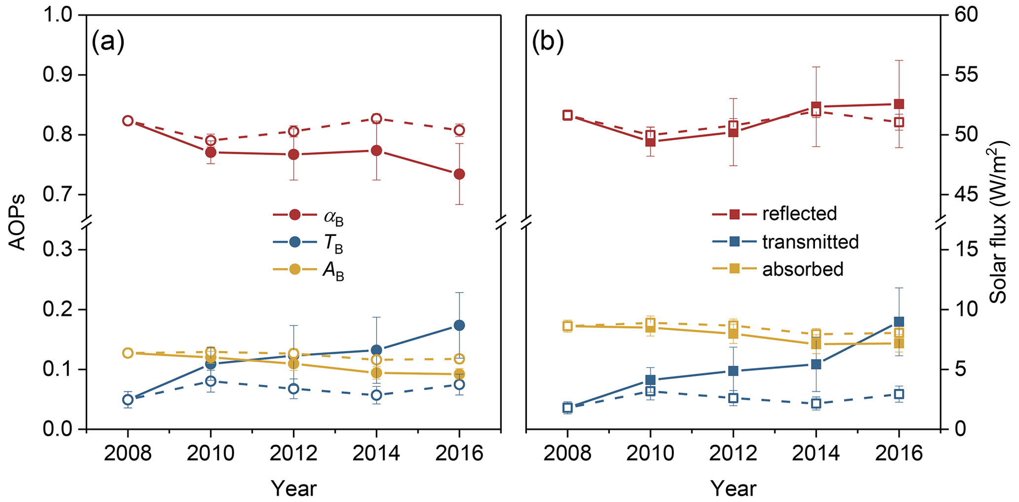
Figure 7Arctic-wide variations in the mean (a) AOPs of ice and (b) solar flux distribution during 2008–2016. Also shown as dashed lines are the AOPs and fluxes with the same IOPs and constant thickness field. The error bars show the standard deviation in each year.
When the ice thickness was set as a constant, variations in the mean AOPs were different, which resulted in differences in the solar flux (dashed lines in Fig. 7b). Among them, differences in the reflected flux Er were relatively small. Meanwhile, the mean Et increased from 1.8 W m−2 in 2008 to 2.9 W m−2 in 2016, with no significant trend. Ea decreased from 8.6 to 8.0 W m−2 in the same period. These changes corresponded to 16.0 % and 39.3 % of the combined effects of the ice IOPs and thickness, respectively, from 2008 to 2016. Furthermore, marginal ice zones with ice thicknesses <1 m still contributed 38.5 % of the increasing Et from 2008 to 2016 (Fig. 8f–j). This value was about 74.3 % of the rate of the combined effects of the changing IOPs and thickness of ice. In other words, the same changes in the ice microstructure had more effects on the TB of thin sea ice, and these effects were clearer than those resulting from general decreasing ice thickness.
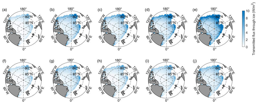
Figure 8Distribution of transmitted solar radiation through sea ice in the summers of 2008 to 2016 when the sea ice thickness was set (a–e) to decrease and (f–j) to a constant value. Only flux that penetrated through the sea ice is considered in these maps.
4.1 Comparisons with IOP measurements
In Sect. 3.2, we estimated the ice IOPs according to the observed ice physics and structural–optical theory. Other methods have been used to estimate ice IOPs in previous studies. In this section, we compare the ice scattering coefficient, the most variable value among IOPs, determined in the present study with previous results (Fig. 9). It is difficult for us to consider the potential affecting factors because the variations in σ were still unclear. So we pay more attention to the comparison of the σ range. The differences in wavelength bands were ignored in the comparisons because σ was nearly wavelength-independent.
It is clear from Fig. 9 that the range of σ of the present study covered the majority of previous results. The derived values of σ for the SSL and DL of melting bare ice in August ranged from 920 to 2000 and 40 to 150 m−1, respectively (Light et al., 2008). According to the layer structure, wherein the TL was composed of a 5 cm SSL and the others were DLs, the bulk σ of the TL in Light et al. (2008) ranged from 270 to 435 m−1. This result was slightly higher than our results. The results of Mobley et al. (1998) and Perron et al. (2021) agree with our range. The σ of the DL in Perron et al. (2021) was in our range, and the values of Light et al. (2008) were smaller than those in the present study.
Differences in the σ of the IL were clearer than in the TL and DL. The σ values of the IL of most our cores were relatively large compared to those of Light et al. (2008, 2015) and Frantz et al. (2019). In these results, Light et al. (2008) estimated the σ using the observed ice albedo and a three-layer structure with fixed thicknesses. The results of Light et al. (2015) and Frantz et al. (2019) were obtained in a cold laboratory by simulating the radiative transport in subsections of sea ice. Meanwhile, the results of Grenfell et al. (2006) and Perron et al. (2021) are close to the minimum of our range. The σ of ice in Grenfell et al. (2006) was calculated from the ice extinction coefficient, and it was measured in situ using a diffuse reflectance probe in Perron et al. (2021). The values calculated by the same method as used in the present study by Mobley et al. (1998) were close to the maximum of our range. Thus, it was expected that the differences in the IL's σ partly resulted from the different methods used in the myriad studies.
One possible reason for the differences was the uncertainties in the ice microstructure introduced by brine loss during measurement and segmenting. Thus, our Va values of the IL are greater than the values derived from nondestructive methods (e.g., Perron et al., 2021). As a result, the maximum underestimate of Vb was 15 %–25 % and the maximum overestimate of Va was 96 %–160 % when taking the uncertainties introduced by the measurements and brine drainage into account (Wang et al., 2020). Taking the mean Va and Vb of all ice cores as an example, these uncertainties overestimated the σ of the IL by 78 m−1 at most. Although brine loss during sampling and measurements introduced uncertainties into Va and Vb, the methods used for obtaining and measuring the ice cores during the CHINARE cruises were the same. Therefore, the uncertainties introduced by the methodology hardly affected the changes seen in Figs. 6 and 7.
Another source of difference is the distribution function of gas bubbles employed in the IOP parameterization. Many distributions are obtained in a cold laboratory, where the ice temperature is not consistent with that in the summer Arctic. As the refractive indices of brine and pure ice were similar, the distribution function of brine pockets had a smaller influence on the ice IOPs than gas bubbles (Yu et al., 2022). Here, we tentatively adjusted the exponent of the distribution function of the gas bubbles from its default value of −1.5 to −1; i.e., the fraction of small bubbles decreases, which coincides with warming ice (Light et al., 2003). Then, the changed distribution function was used for 1 m thick ice with mean values of Va and Vb for every ice core. This change resulted in an uncertainty of 8 m−1 in the σ of each layer. These uncertainties did not alter the above results and are considered acceptable.
Although brine loss and the difference in the distribution functions of gas bubbles introduced uncertainties into σ, they did not affect the ice AOPs much. Considering a 1 m thick ice layer described by the mean physics of ice cores, the effects of the former factor on the ice AOPs were less than 0.02. The uncertainties in αB and TB introduced by the latter factor were 0.005 and 0.002, respectively. Therefore, our estimated αB range (0.76–0.87) agreed with the observed results of Light et al. (2008, 2015) and Grenfell et al. (2006). Meanwhile, the estimated TB (0.01–0.1) was also in the corresponding observed ranges.
4.2 On the potential interannual variations in the IOPs
Extensive measurements of the IOPs of Arctic sea ice have been carried out, and some authors have noticed the seasonal variations in the ice microstructure and IOPs (Light et al., 2008; Frantz et al., 2019; Katlein et al., 2021). However, if there are interannual variations in sea ice IOPs is still not clear, although such changes in sea ice extent, thickness, and age are evident. A lack of continuous IOP measurements is the primary reason. Compared with previous observations, the ice core data in the present study were more appropriate for analyses on the potential interannual variations in ice IOPs because of their long time span and consistencies in the sampling method, seasons, and sea areas. The reason we could not introduce other ice core data (SHEBA, ICESCAPE, N-ICE, MOSAiC, etc.) into this study was that not only do the differences in sampling seasons, sites, and methods increase the dispersion in time and space during such an analysis, but also the lack of information about the ice microstructure or essential physical properties will limit how much we can determine from such a comparison. We consider the presented ice core data to comprise the best possible estimate on the potential interannual variations at this time while acknowledging that further improvements of the data products are needed. Considering that sampling ice cores is a commonly used method for in situ observations, with more suitable ice core data in the future, large-scale time series of ice IOPs may be obtained.
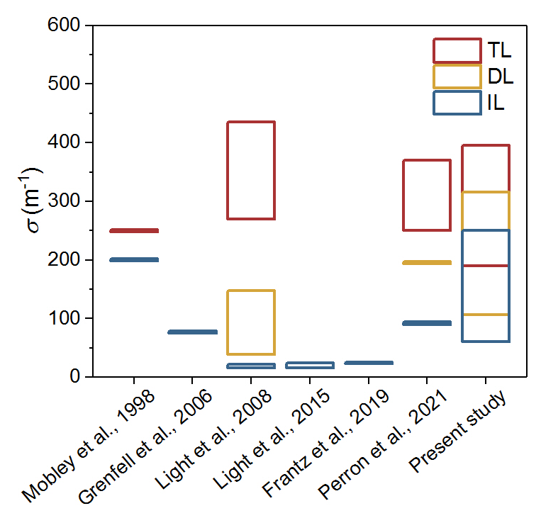
Figure 9Comparison of the ice scattering coefficient in the present study to the published results for Arctic sea ice using various methods. All comparison results have been scaled to the layer structure used in the current study according to their ice thicknesses.
The ice cores used in the present study were sampled at different ice stations but not at the same floe (Fig. 1). That is, the data did not form a continuous observation in the strictest meaning. Thus, the variations shown in Sect. 3 can be regarded as the combined effects from three parts, i.e., spatial, temporal, and interannual variations. To discuss interannual variability, it is necessary to first establish the spatial and temporal variability in ice cores. Figure 10 illustrates the different IOPs of the ice cores in three latitude zones, which shows that there are spatial differences in the present ice core data. Among the three IOPs, variations in σ are the clearest (up to 20 %, Fig. 10a). The differences in κB and g in the different latitude zones were not more than 5 % and 3 %, respectively (Fig. 10b, c). As a transition layer between the TL and IL, variations in the IOPs of the DL were more discrete than in the other two layers. For now, we have little quantitative knowledge of the progressions of the sea ice IOPs and their influencing factors in the available literature. In the following discussion, the σ was set as the main content.
It can be seen from Fig. 10a that there were no clear changes in the mean σ of TL in different latitude zones. Therefore, we ignore the spatial variations in σ of the TL. We further discuss all its variations in different years. The variability in the ice surface is directly related to the number of melt days. The melt days are affected by the radiation balance, water vapor, air temperature, and other factors (Persson, 2012; Crawford et al., 2018; Mortin et al., 2016). Figure 11a shows the data obtained from ECMWF: the downward longwave radiation was 300.2 ± 4.0 W m−2 at the surface during the study years with no statistically significant trend (, P>0.1). The total column vertically integrated water vapor was also similar (11.9 ± 0.4 kg m−2) with no significant trend (, P>0.1). Differently from the surface radiation, we found the observed air temperature increased at a speed of 0.14∘ yr−1 (r=0.84, P<0.1, Fig. 11a). This clear difference in the temperatures was not an exception but a general circumstance in the Arctic during 2008–2016 (Collow et al., 2020). This could also be seen in the reanalysis data of ECMWF, where the mean air temperature in the summer of the study area has been increasing gradually (0.12∘ yr−1, r=0.84, P<0.1). With the effects of several factors, the melting days of sampling sites, which were calculated according to the sampling date and melt onset from Markus et al. (2009), totaled 59 ± 7 d (Fig. 11a). Their variation between years was statistically insignificant (ANOVA, P>0.1). In other words, there are no significant differences in the surface melt of the ice cores in different years.
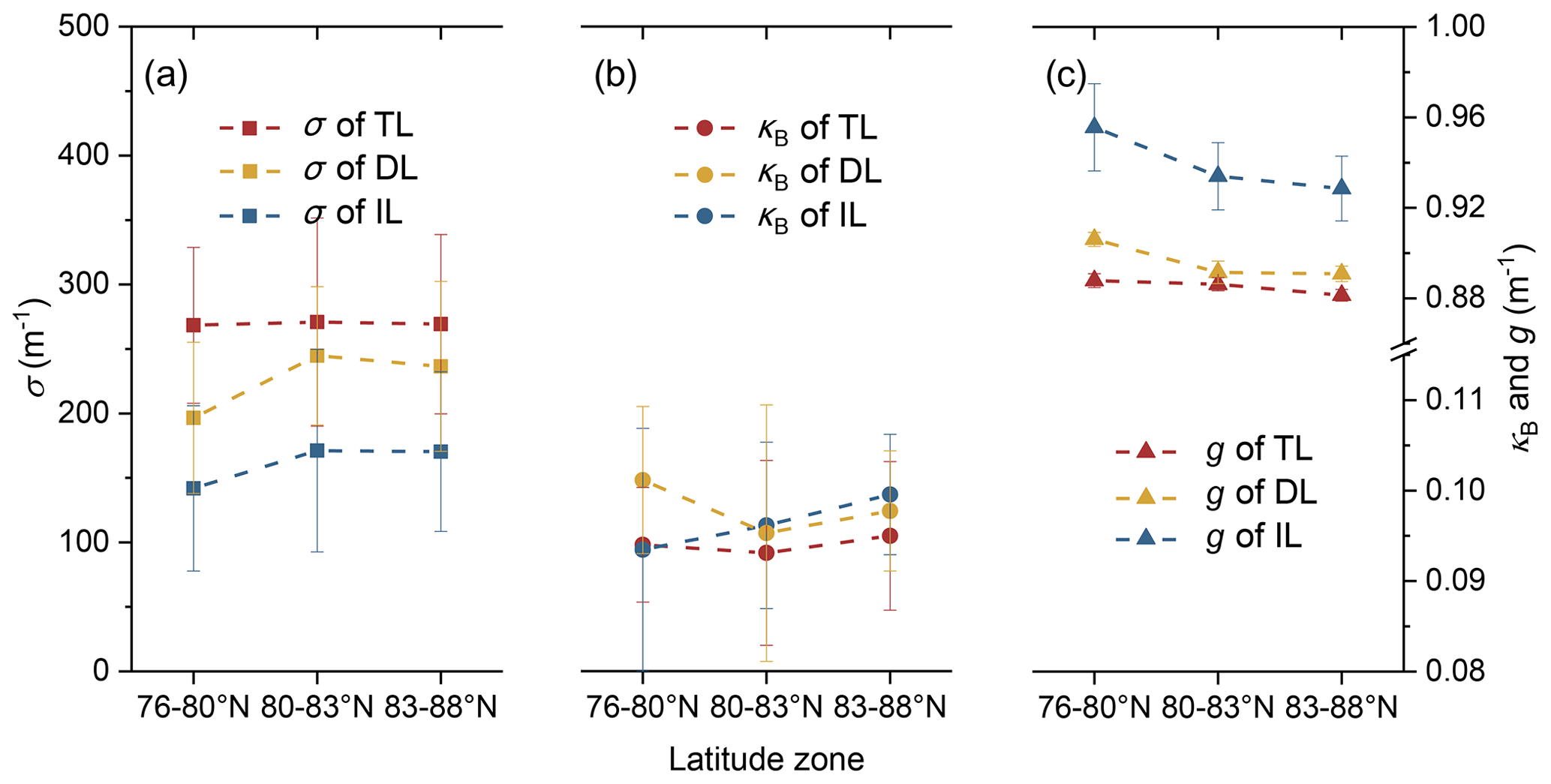
Figure 10Different values of (a) σ, (b) κB, and (c) g for the TL, DL, and IL of the ice cores in the three latitude zones. The error bars show the standard deviation in each latitude zone.
Previous observations demonstrated that ice surface melt was relatively weak in August (Nicolaus et al., 2021; Perovich, 2003b). Macfarlane et al. (2023) further found that the SSL microstructure of melting ice had no temporal changes. Meanwhile, the differences in longwave radiation and vapor between sampling sites in single years were relatively small (Fig. 11a). So it is expected that the scattering coefficient of the TL also has no clear seasonal variations, whereas an increasing scattering in the SSL during the melt season was found in Light et al. (2008). This seems contrary to the findings of Macfarlane et al. (2023), but it is not. As stated in Light et al. (2008), the observed increase in scattering represents not only an increased scattering in a fixed depth layer but also an increased physical depth of the SSL or increased scattering of the next ice layer because the modeled layer thickness is fixed. What was the same in the two studies was approximately constant albedo (or reflectance). This agrees with the similar albedo in Fig. 6b of the present study; i.e., small seasonal differences do not affect the reflectivity of bare ice. Up until now, there has been no theoretical explanation or quantitative description of the evolution of the microstructure of the ice surface during the melt (Petrich and Eicken, 2010). It can be seen from the present result that the increasing air temperature does not seem to be the predominant affecting factor in the late melting season. In short, it is expected that the effects of temporal variations on the microstructure and IOPs of the ice surface are relatively small. Considering that all the variations in microstructure (Fig. 3) and IOPs (Fig. 5) were not significant, there are no clear temporal, spatial, or interannual variations in the ice surface of the present ice core data.
The σ of the IL is relatively constant during the entire melt season (Light et al., 2008). That is to say, all the variations in the ice interior layer did not result from temporal factors. Meanwhile, the latitudinal differences in the σ of the IL are clear. The σ of the ice IL in the low-latitude zone was relatively small compared to that in middle- or high-latitude zones (Fig. 10a). It is expected that the ice at lower latitudes is generally warmer earlier, which increases the brine inclusion size and connectivity of ice. This naturally reduces the ice scattering coefficient. The spatial variation in mean σ in the IL can be up to 30 m−1 between low-latitude and middle- or high-latitude zones. This value is equivalent to 32.9 % of the maximum of the whole variation. This implies that the spatial and interannual variations in ice properties together result in the changing IOPs shown in Fig. 5. So it is necessary to exclude the spatial variations before discussing the interannual changes in σ. According to the propagation law of variation, the square of all the variations in IL σ can be expressed as the square sum of their spatial variations and interannual variations. For the convenience of calculation, we ignored the small difference in IL σ between middle- and high-latitude zones. There are five and three cores from 2014 and 2016 sampled in the low-latitude zone, respectively. According to the differences between ice cores from different years (all variations, Fig. 3) and different latitude zones (spatial variations, Fig. 10a), we correct the mean σ of the IL in 2014 from 176 to 182 m−1. That is to say, the interannual variations were larger than all the variations by 6 m−1. The value of 2016 was also corrected from 127 to 131 m−1 accordingly. Then, variations among the corrected σ of the IL could be regarded as the result of the interannual factors.
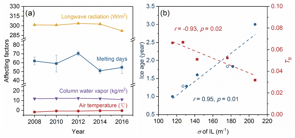
Figure 11(a) Changing melting days, surface downward longwave radiation flux, total column vertically integrated water vapor, and observed air temperature at the sampling sites. The error bars show the standard deviation in each year. Some error bars are invisible because they are small. (b) Correlations among the σ values of the IL with ice age and TB. The circles denote the uncorrected data.
Then, the corrected σ of the IL was used to discuss the interannual changes. Figure 11b shows the correlations among the corrected σ of the IL, ice age, and TB in study years. Also shown in circles are the uncorrected σ of the IL in 2014 and 2016. Note that TB here is the result obtained under the assumption of a constant ice thickness (dashed line in Fig. 6c). The ice ages were obtained according to fieldwork (Wang et al., 2020) and remote-sensing data (Tschudi et al., 2019). Because the ice age of each grid cell in the remote-sensing data is represented as the age of the oldest floe, once an ice core was distinguished as first-year ice in the fieldwork, the corresponding ice age was set as 1 year regardless of the remote-sensing data. The use of remote-sensing data is acceptable because the ice cores in this study were all sampled in large and thick floes for safe fieldwork. These floes were more likely older than the surrounding ice. Figure 11b demonstrates that the decrease in the σ of the IL is significantly correlated with changing ice age (r=0.95, P<0.01). In other words, the ice age was largely manifested in the ice microstructure in the IL. A similar result was also observed: the σ of the IL in the first-year ice was smaller than in multiyear ice (e.g., Light et al., 2015). This could also partly explain the spatial variations in the σ of the IL (Fig. 10a) because sea ice in high-latitude zones was likely older than in the other zones (Stroeve and Notz, 2018). Furthermore, there are significant correlations between σ of the IL and ice TB (, P<0.05). That is to say, the changing ice age can be responsible for the modeled results of changing ice transmittance shown in Fig. 7, even without any decrease in the ice thickness. One other thing to point out is that the changing ice age does not seem to affect the albedo of bare ice (Fig. 6b). Light et al. (2022) suggest that the principal reason for this is the SSL shows invariance across location, decade, and ice age, which was confirmed by comparing data from MOSAiC (2019–2020) and SHEBA (1997–1998). Our results partly prove this view; i.e., there are significant variations in the ice age but no significant variations in microstructure or IOPs of the TL during 2008–2016.
In summary, we did not find significant variations in the IOPs of the ice top layer. Meanwhile, the differences in the IOPs of the ice IL were related to interannual variations in the ice age. To our knowledge, this is the first study to link ice microstructure and optical properties at interannual scales. Although these ice core data are not a time series in the strictest meaning, they are still helpful for understanding the general effects of the scenario where the Arctic ice ages are decreasing. Our results suggest that in this scenario, the σ values of the IL of summer ice tend to be smaller than before. This is expected to lead to interannual trends of the ice microstructure and IOPs. Then, more solar radiation is transmitted into the ocean. The effects of this process need more attention in future observations and simulations.
4.3 Implications for the future Arctic
Previous studies have reported that surface properties (snow, ponds, etc.) largely control the variations in the ice albedo (Landy et al., 2015). The present results also indicate that variations in the ice's microstructure or IOPs had little effect on the albedo of bare ice (<2 %), but they do play an important role in ice transmittance (Fig. 6). With continued Arctic warming, the summer ice age is on the decrease, and the ice microstructure and IOPs change accordingly, leading to an overall higher ice transmittance. Furthermore, the transmitted solar energy affects the temperature of the upper ocean and results in further melting of the bottom of sea ice (Timmermans, 2015). Along with the melting of ice, gas bubbles, and brine pockets change simultaneously (Light et al., 2004), which affects the IOPs of ice in turn. Consequently, the sea ice is expected to become thinner and more porous than before. This process has been seldom considered in previous studies. Related studies have generally regarded the surface properties and thickness of the ice as predictors for light transmittance (Katlein et al., 2015; Perovich et al., 2020). The microstructure and morphological parameters of sea ice (e.g., thickness, extent) may together influence the melting processes of Arctic sea ice.
For safe field observations, the ice core data used in this study were all sampled in large and thick floes. Therefore, variations in the microstructure of the ice in marginal zones or under melt ponds cannot be addressed by this study. Light et al. (2015) reported that the differences in the σ between the IL of ponded first-year ice and multiyear ice were larger than those between bare first-year ice and multiyear ice. Therefore, the changes in the IOPs of the marginal ice zone were expected to be more obvious than those found in the present results because the ice in marginal zones is more likely young and ponded (Rigor and Wallace, 2004; Zhang et al., 2018). Furthermore, the same changes in the ice microstructure have more effects on the TB of thin sea ice (Sect. 3.4). Marginal ice zones, comprising 16.4 % of the entire ice area, contributed 39.3 % of the extra transmitted solar energy due to the changing ice microstructure from 2008 to 2016 (Fig. 8). Both processes promote an increase in transmitted flux through sea ice and ice bottom melting in marginal ice zones. Arndt and Nicolaus (2014) quantified light transmittance through the sea ice into the ocean for all seasons as a function of variable sea ice types. The mean annual trend was 1.5 % yr−1, which mainly depended on the timing of melt onset. If the variations in the microstructure of bare and ponded ice are taken into consideration, this trend is expected to increase. We suggest that future ice observations and models should pay more attention to variations in the ice age, microstructure, and their effects, especially in marginal ice zones.
We want to emphasize the Arctic basin-scale analysis is a highly idealized investigation. To obtain a real distribution of the transmitted solar radiation through sea ice in the Arctic basin scale in the summer is far more complicated and would require a massive amount of ice core sampling collected simultaneously in various parts of the Arctic Ocean. Such field expeditions will not be able to be arranged anytime soon in the future. We intend to provide one possible scenario of IOPs. We call for further strengthening international collaborations to make possible a better understanding of the Arctic IOP distribution.
This is the first study to link the ice microstructure, IOPs, and AOPs at interannual scales. Based on ice cores sampled during the CHINARE expeditions (2008–2016), the variations in the IOPs of Arctic sea ice in summer due to the changing microstructure of ice were modeled according to structural–optical theory. Variations in the AOPs and solar flux distribution due to the changing IOPs in the summer Arctic were also estimated. Clear variations in the microstructure and IOPs of each year (Fig. 5) enabled us to construct a quantitative view of changes that the Arctic sea ice interior underwent in these years.
As a result of our study, there were no significant variations in the microstructure and IOPs of the ice TL. This is related to the stable melt days in study years. Because σ values of the upper layers (TL and DL) mainly control the albedo of bare ice, the variations in αB between years were relatively small. Meanwhile, variations in the microstructure and IOPs of the IL were significant. These variations consist mainly of interannual factors and minor spatial factors. After excluding the effects of spatial variations, we found these interannual variations in σ of the ice IL were highly related to the changing ice ages. That is to say, the ice age largely manifested in the ice microstructure of the IL. The changing σ of the ice IL affects the ice transmittance clearly. Furthermore, the same changes in the ice IOPs had more effects on the transmittance of the thin ice in marginal ice zones.
Previous studies have paid more attention to changing transmittance due to declining ice thickness. The present findings demonstrate that the changing IOPs of interior ice derived from the ice microstructure could also alter the partitioning of solar radiation in sea ice by itself. With continued Arctic warming, summer ice will become younger and more porous than before, leading to more light reaching the upper ocean. This reminds us to pay more attention to the variations in the IOPs of interior ice, especially ice with different ages.
The sea ice and radiation data are available at https://doi.org/10.5067/MPYG15WAA4WX (DiGirolamo et al., 2022), https://data.meereisportal.de/relaunch/thickness?lang=en (Ricker et al., 2017), and https://doi.org/10.24381/cds.f17050d7 (Hersbach et al., 2023). The ice core data applied in this work can be accessed at https://doi.org/10.1029/2020JC016371 (Wang et al., 2020).
The supplement related to this article is available online at: https://doi.org/10.5194/tc-18-273-2024-supplement.
MY carried out the estimations and wrote the paper. RL, BL, and QW provided the ice core data. All co-authors discussed the results and edited the manuscript.
At least one of the (co-)authors is a member of the editorial board of The Cryosphere. The peer-review process was guided by an independent editor, and the authors also have no other competing interests to declare.
Publisher’s note: Copernicus Publications remains neutral with regard to jurisdictional claims made in the text, published maps, institutional affiliations, or any other geographical representation in this paper. While Copernicus Publications makes every effort to include appropriate place names, the final responsibility lies with the authors.
We would like to thank the handing editor Marie Dumont and the four anonymous reviewers. Their criticism and constructive comments helped to improve this paper significantly. We are grateful to the NSIDC, Alfred Wegener Institute, and ECMWF for providing the sea ice and radiation data. This work was financially supported by the National Key Research and Development Program of China (grant number 2018YFA0605901), the National Natural Science Foundation of China (grant numbers 41922045, 41906198, 41976219, and 41876213), and the Academy of Finland (grant numbers 333889, 325363, and 317999). We also wish to acknowledge the crews of the R/V Xuelong for their fieldwork during CHINARE.
This research has been supported by the National Key Research and Development Program of China (grant no. 2018YFA0605901), the National Natural Science Foundation of China (grant nos. 41922045, 41906198, 41976219, and 41876213), and the Academy of Finland (grant nos. 333889, 325363, and 317999).
This paper was edited by Marie Dumont and reviewed by four anonymous referees.
Arndt, S. and Nicolaus, M.: Seasonal cycle and long-term trend of solar energy fluxes through Arctic sea ice, The Cryosphere, 8, 2219–2233, https://doi.org/10.5194/tc-8-2219-2014, 2014.
Briegleb, B. P. and Light, B.: A Delta-Eddington Multiple Scattering Parameterization for Solar Radiation in the Sea Ice Component of the Community Climate System Model (No. NCAR/TN-472+STR), University Corporation for Atmospheric Research, https://doi.org/10.5065/D6B27S71, 2007.
Carnat, G., Papakyriakou, T., Geilfus, N. X., Brabant, F., Delille, B., Vancoppenolle, M., Gilson, G., Zhou, J., and Tison, J.: Investigations on physical and textural properties of Arctic first-year sea ice in the Amundsen Gulf, Canada, November 2007–June 2008 (IPY-CFL system study), J. Glaciol., 59, 819–837, https://doi.org/10.3189/2013JoG12J148, 2013.
Cole, D. M., Eicken, H., Frey, K., and Shapiro, L. H.: Observations of banding in first-year Arctic sea ice, J. Geophys. Res.-Oceans, 109, C08012, https://doi.org/10.1029/2003JC001993, 2004.
Collow, A. B., Cullather, R. I., and Bosilovich, M. G.: Recent Arctic Ocean Surface Air Temperatures in Atmospheric Reanalyses and Numerical Simulations, J. Climate, 33, 4347–4367, https://doi.org/10.1175/JCLI-D-19-0703.1, 2020.
Comiso, J. C., Parkinson, C. L., Gersten, R., and Stock, L.: Accelerated decline in the Arctic sea ice cover, Geophys. Res. Lett., 35, L1703, https://doi.org/10.1029/2007GL031972, 2008.
Crabeck, O., Galley, R., Delille, B., Else, B., Geilfus, N.-X., Lemes, M., Des Roches, M., Francus, P., Tison, J.-L., and Rysgaard, S.: Imaging air volume fraction in sea ice using non-destructive X-ray tomography, The Cryosphere, 10, 1125–1145, https://doi.org/10.5194/tc-10-1125-2016, 2016.
Crabeck, O., Galley, R. J., Mercury, L., Delille, B., Tison, J. L., and Rysgaard, S.: Evidence of Freezing Pressure in Sea Ice Discrete Brine Inclusions and Its Impact on Aqueous Gaseous Equilibrium, J. Geophys. Res.-Oceans, 124, 1660–1678, https://doi.org/10.1029/2018JC014597, 2019.
Crawford, A. D., Horvath, S., Stroeve, J., Balaji, R., and Serreze, M. C.: Modulation of Sea Ice Melt Onset and Retreat in the Laptev Sea by the Timing of Snow Retreat in the West Siberian Plain, J. Geophys. Res.-Atmos., 123, 8691–8707, https://doi.org/10.1029/2018JD028697, 2018.
Dai, A., Luo, D., Song, M., and Liu, J.: Arctic amplification is caused by sea-ice loss under increasing CO2, Nat. Commun., 10, 121, https://doi.org/10.1038/s41467-018-07954-9, 2019.
DiGirolamo, N. E., Parkinson, C., Cavalieri, D. J., Gloersen, P., and Zwally, H. J.: updated yearly, Sea Ice Concentrations from Nimbus-7 SMMR and DMSP SSM/I-SSMIS Passive Microwave 40 Data, Version 2, Boulder, Colorado USA, NASA National Snow and Ice Data Center Distributed Active Archive Center, https://doi.org/10.5067/MPYG15WAA4WX, 2022.
Ehn, J. K., Papakyriakou, T. N., and Barber, D. G.: Inference of optical properties from radiation profiles within melting landfast sea ice, J. Geophys. Res., 113, C9024, https://doi.org/10.1029/2007JC004656, 2008.
Eicken, H., Lensu, M., Leppäranta, M., Tucker, W. B., Gow, A. J., and Salmela, O.: Thickness, structure, and properties of level summer multiyear ice in the Eurasian sector of the Arctic Ocean, J. Geophys. Res., 100, 22697–22710, https://doi.org/10.1029/95JC02188, 1995.
Eicken, H., Grenfell, T. C., Perovich, D. K., Richter-Menge, J. A., and Frey, K.: Hydraulic controls of summer Arctic pack ice albedo, J. Geophys. Res.-Oceans, 109, https://doi.org/10.1029/2003JC001989, 2004.
Frantz, C. M., Light, B., Farley, S. M., Carpenter, S., Lieblappen, R., Courville, Z., Orellana, M. V., and Junge, K.: Physical and optical characteristics of heavily melted “rotten” Arctic sea ice, The Cryosphere, 13, 775–793, https://doi.org/10.5194/tc-13-775-2019, 2019.
Grenfell, T. C.: A theoretical model of the optical properties of sea ice in the visible and near infrared, J. Geophys. Res.-Oceans, 88, 9723–9735, https://doi.org/10.1029/JC088iC14p09723, 1983.
Grenfell, T. C.: A radiative transfer model for sea ice with vertical structure variations, J. Geophys. Res.-Oceans,, 96, 16991–17001, https://doi.org/10.1029/91JC01595, 1991.
Grenfell, T. C. and Perovich, D. K.: Radiation Absorption Coefficients of Polycrystalline ice from 400 to 1400 nm, J. Geophys. Res., 86, 7447–7450, https://doi.org/10.1029/2007JD009744, 1981.
Grenfell, T. C. and Warren, S. G.: Representation of a nonspherical ice particle by a collection of independent spheres for scattering and absorption of radiation, J. Geophys. Res., 104, 31697–31709, https://doi.org/10.1029/1999JD900496, 1999.
Grenfell, T. C. and Perovich, D. K.: Incident spectral irradiance in the Arctic Basin during the summer and fall, J. Geophys. Res., 113, D12117, https://doi.org/10.1029/2007JD009418, 2008.
Grenfell, T. C., Light, B., and Perovich, D. K.: Spectral transmission and implications for the partitioning of shortwave radiation in arctic sea ice, Ann. Glaciol., 44, 1–6, https://doi.org/10.3189/172756406781811763, 2006.
Hamre, B.: Modeled and measured optical transmittance of snow-covered first-year sea ice in Kongsfjorden, Svalbard, J. Geophys. Res., 109, C10006, https://doi.org/10.1029/2003JC001926, 2004.
Hansen, J. E. and Travis, L. D.: Light scattering in planetary atmosphere, Space Sci. Rev., 16, 527–610, https://doi.org/10.1007/BF00168069, 1974.
Hersbach, H., Bell, B., Berrisford, P., Biavati, G., Horányi, A., Muñoz Sabater, J., Nicolas, J., Peubey, C., Radu, R., Rozum, I., Schepers, D., Simmons, A., Soci, C., Dee, D., and Thépaut, J.-N.: ERA5 monthly averaged data on single levels from 1940 to present, Copernicus Climate Change Service (C3S) Climate Data Store (CDS), https://doi.org/10.24381/cds.f17050d7, 2023.
Hunke, E. C., Notz, D., Turner, A. K., and Vancoppenolle, M.: The multiphase physics of sea ice: a review for model developers, The Cryosphere, 5, 989–1009, https://doi.org/10.5194/tc-5-989-2011, 2011.
Katlein, C., Arndt, S., Nicolaus, M., Perovich, D. K., Jakuba, M. V., Suman, S., Elliott, S., Whitcomb, L. L., McFarland, C. J., Gerdes, R., Boetius, A., and German, C. R.: Influence of ice thickness and surface properties on light transmission through Arctic sea ice, J. Geophys. Res.-Oceans, 120, 5932–5944, https://doi.org/10.1002/2015JC010914, 2015.
Katlein, C., Arndt, S., Belter, H. J., Castellani, G., and Nicolaus, M.: Seasonal Evolution of Light Transmission Distributions Through Arctic Sea Ice, J. Geophys. Res.-Oceans, 124, 5418–5435, https://doi.org/10.1029/2018JC014833, 2019.
Katlein, C., Valcic, L., Lambert-Girard, S., and Hoppmann, M.: New insights into radiative transfer within sea ice derived from autonomous optical propagation measurements, The Cryosphere, 15, 183–198, https://doi.org/10.5194/tc-15-183-2021, 2021.
Kwok, R.: Arctic sea ice thickness, volume, and multiyear ice coverage: losses and coupled variability (1958–2018), Environ. Res. Lett., 13, 105005, https://doi.org/10.1088/1748-9326/aae3ec, 2018.
Kwok, R. and Cunningham, G. F.: Contributions of growth and deformation to monthly variability in sea ice thickness north of the coasts of Greenland and the Canadian Arctic Archipelago, Geophys. Res. Lett., 43, 8097–8105, https://doi.org/10.1002/2016GL069333, 2016.
Landy, J. C., Ehn, J. K., and Barber, D. G.: Albedo feedback enhanced by smoother Arctic sea ice, Geophys. Res. Lett., 42, 710–714, https://doi.org/10.1002/2015GL066712, 2015.
Lei, R., Tian-Kunze, X., Leppäranta, M., Wang, J., Kaleschke, L., and Zhang, Z.: Changes in summer sea ice, albedo, and portioning of surface solar radiation in the Pacific sector of Arctic Ocean during 1982–2009, J. Geophys. Res.-Oceans, 121, 5470–5486, https://doi.org/10.1002/2016JC011831, 2016.
Light, B., Maykut, G. A., and Grenfell, T. C.: Effects of temperature on the microstructure of first-year Arctic sea ice, J. Geophys. Res.-Oceans, 108, 3051, https://doi.org/10.1029/2001JC000887, 2003.
Light, B., Maykut, G. A., and Grenfell, T. C.: A temperature-dependent, structural-optical model of first-year sea ice, J. Geophys. Res., 109, C6013, https://doi.org/10.1029/2003JC002164, 2004.
Light, B., Grenfell, T. C., and Perovich, D. K.: Transmission and absorption of solar radiation by Arctic sea ice during the melt season, J. Geophys. Res., 113, C3023, https://doi.org/10.1029/2006JC003977, 2008.
Light, B., Perovich, D. K., Webster, M. A., Polashenski, C., and Dadic, R.: Optical properties of melting first year Arctic sea ice, J. Geophys. Res.-Oceans,, 120, 7657–7675, https://doi.org/10.1002/2015JC011163, 2015.
Light, B., Smith, M. M., Perovich, D. K., Webster, M. A., Holland, M. M., Linhardt, F., Raphael, I. A., Clemens-Sewall, D., Macfarlane, A. R., Anhaus, P., and Bailey, D. A.: Arctic sea ice albedo: Spectral composition, spatial heterogeneity, and temporal evolution observed during the MOSAiC drift, Elementa, 10, 000103, https://doi.org/10.1525/elementa.2021.000103, 2022.
Lindsay, R. and Schweiger, A.: Arctic sea ice thickness loss determined using subsurface, aircraft, and satellite observations, The Cryosphere, 9, 269–283, https://doi.org/10.5194/tc-9-269-2015, 2015.
Macfarlane, A. R., Dadic, R., Smith, M. M., Light, B., Nicolaus, M., Henna-Reetta, H., Webster, M., Linhardt, F., Hämmerle, S., and Schneebeli, M.: Evolution of the microstructure and reflectance of the surface scattering layer on melting, level Arctic sea ice, Elementa, 11, 00103, https://doi.org/10.1525/elementa.2022.00103, 2023.
Markus, T., Stroeve, J. C., and Miller, J.: Recent changes in Arctic sea ice melt onset, freezeup, and melt season length, J. Geophys. Res., 114, C12024, https://doi.org/10.1029/2009JC005436, 2009.
Mobley, C. D., Cota, G. F., Grenfell, T. C., Maffione, R. A., Pegau, W. S., and Perovich, D. K.: Modeling Light Propagation in Sea Ice, IEEE T. Geosci. Remote, 36, 1743–1749, https://doi.org/10.1109/36.718642, 1998.
Mortin, J., Svensson, G., Graversen, R. G., Kapsch, M., Stroeve, J. C., and Boisvert, L. N.: Melt onset over Arctic sea ice controlled by atmospheric moisture transport, Geophys. Res. Lett., 43, 6636–6642, https://doi.org/10.1002/2016GL069330, 2016.
Nicolaus, M., Hoppmann, M., Arndt, S., Hendricks, S., Katlein, C., Nicolaus, A., Rossmann, L., Schiller, M., and Schwegmann, S.: Snow depth and air temperature seasonality on sea ice derived from snow buoy measurements, Front. Mar. Sci., 8, 655446, https://doi.org/10.3389/fmars.2021.655446, 2021.
Notz, D. and Worster, M. G.: Desalination processes of sea ice revisited, J. Geophys. Res., 114, C05006, https://doi.org/10.1029/2008JC004885, 2009.
Parkinson, C. L. and Comiso, J. C.: On the 2012 record low Arctic sea ice cover: Combined impact of preconditioning and an August storm, Geophys. Res. Lett., 40, 1356–1361, https://doi.org/10.1002/grl.50349, 2013.
Perovich, D. K.: Complex yet translucent: the optical properties of sea ice, Physica B, 338, 107–114, https://doi.org/10.1016/S0921-4526(03)00470-8, 2003a.
Perovich, D. K.: Thin and thinner: Sea ice mass balance measurements during SHEBA, J. Geophys. Res., 108, 8050, https://doi.org/10.1029/2001JC001079, 2003b.
Perovich, D., Light, B., and Dickinson, S.: Changing ice and changing light: trends in solar heat input to the upper Arctic ocean from 1988 to 2014, Ann. Glaciol., 61, 401–407, https://doi.org/10.1017/aog.2020.62, 2020.
Perron, C., Katlein, C., Lambert-Girard, S., Leymarie, E., Guinard, L.-P., Marquet, P., and Babin, M.: Development of a diffuse reflectance probe for in situ measurement of inherent optical properties in sea ice, The Cryosphere, 15, 4483–4500, https://doi.org/10.5194/tc-15-4483-2021, 2021.
Persson, P. O. G.: Onset and end of the summer melt season over sea ice: thermal structure and surface energy perspective from SHEBA, Clim. Dynam., 39, 1349–1371, https://doi.org/10.1007/s00382-011-1196-9, 2012.
Petrich, C. and Eicken, H.: Growth, Structure and Properties of Sea Ice, in: Sea ice, edited by: Thomas, D. N., Dieckmann, G. S., 2nd ed. Hoboken, NJ: Wiley Online Library, 23–77, 2010.
Petty, A. A., Stroeve, J. C., Holland, P. R., Boisvert, L. N., Bliss, A. C., Kimura, N., and Meier, W. N.: The Arctic sea ice cover of 2016: a year of record-low highs and higher-than-expected lows, The Cryosphere, 12, 433–452, https://doi.org/10.5194/tc-12-433-2018, 2018.
Ricker, R., Hendricks, S., Kaleschke, L., Tian-Kunze, X., King, J., and Haas, C.: A weekly Arctic sea-ice thickness data record from merged CryoSat-2 and SMOS satellite data, The Cryosphere, 11, 1607–1623, https://doi.org/10.5194/tc-11-1607-2017, 2017.
Rigor, I. G. and Wallace, J. M.: Variations in the age of Arctic sea-ice and summer sea-ice extent, Geophys. Res. Lett., 31, https://doi.org/10.1029/2004GL019492, 2004.
Smedley, A. R. D., Evatt, G. W., Mallinson, A., and Harvey, E.: Solar radiative transfer in Antarctic blue ice: spectral considerations, subsurface enhancement, inclusions, and meteorites, The Cryosphere, 14, 789–809, https://doi.org/10.5194/tc-14-789-2020, 2020.
Smith, M. M., Light, B., Macfarlane, A. R., Perovich, D. K., Holland, M. M., and Shupe, M. D.: Sensitivity of the Arctic Sea Ice Cover to the Summer Surface Scattering Layer, Geophys. Res. Lett., 49, e2022GL098349, https://doi.org/10.1029/2022GL098349, 2022.
Smith, R. C. and Baker, K. S.: Optical properties of the clearest natural waters (200–800 nm), Appl. Opt., 20, 177, https://doi.org/10.1364/AO.20.000177, 1981.
Stroeve, J. and Notz, D.: Changing state of Arctic sea ice across all seasons, Environ. Res. Lett., 13, 103001, https://doi.org/10.1088/1748-9326/aade56, 2018.
Timmermans, M. L.: The impact of stored solar heat on Arctic sea ice growth, Geophys. Res. Lett., 42, 6399–6406, https://doi.org/10.1002/2015GL064541, 2015.
Tschudi, M. A., Meier, W. N., and Stewart, J. S.: An enhancement to sea ice motion and age products at the National Snow and Ice Data Center (NSIDC), The Cryosphere, 14, 1519–1536, https://doi.org/10.5194/tc-14-1519-2020, 2020.
Tschudi, M., Meier, W., Stewart, J. S., Fowler, C., and Maslanik, J.: EASE-Grid Sea Ice Age, Version 4, Indicate subset used, Boulder, Colorado USA, NASA National Snow and Ice Data Center Distributed Active Archive Center, https://doi.org/10.5067/UTAV7490FEPB, 2019.
Tucker III, W. B., Perovich, D. K., Gow, A. J., Weeks, W. F., and Drinkwater, M. R.: Physical Properties of Sea Ice Relevant to Remote Sensing, in: Microwave Remote Sensing of Sea Ice, American Geophysical Union, 9–28, edited by: Carsey, F. D., https://doi.org/10.1029/GM068p0009, 1992.
Vancoppenolle, M., Fichefet, T., and Goosse, H.: Simulating the mass balance and salinity of Arctic and Antarctic sea ice, 2. Importance of sea ice salinity variations, Ocean Model., 27, 54–69, https://doi.org/10.1016/j.ocemod.2008.11.003, 2009.
Veyssière, G., Castellani, G., Wilkinson, J., Karcher, M., Hayward, A., Stroeve, J. C., Nicolaus, M., Kim, J., Yang, E., Valcic, L., Kauker, F., Khan, A. L., Rogers, I., and Jung, J.: Under-Ice Light Field in the Western Arctic Ocean During Late Summer, Front. Earth Sci., 9, 643737, https://doi.org/10.3389/feart.2021.643737, 2022.
Wang, Q., Lu, P., Leppäranta, M., Cheng, B., Zhang, G., and Li, Z.: Physical Properties of Summer Sea Ice in the Pacific Sector of the Arctic During 2008–2018, J. Geophys. Res.-Oceans, 125, e2020JC016371, https://doi.org/10.1029/2020JC016371, 2020.
Weeks, W. F. and Ackley, S. F.: The Growth, Structure, and Properties of Sea Ice, https://doi.org/10.1007/978-1-4899-5352-0_2, 1986.
Yu, M., Lu, P., Cheng, B., Leppäranta, M., and Li, Z.: Impact of Microstructure on Solar Radiation Transfer Within Sea Ice During Summer in the Arctic: A Model Sensitivity Study, Front. Mar. Sci., 9, 861994, https://doi.org/10.3389/fmars.2022.861994, 2022.
Zhang, J., Schweiger, A., Webster, M., Light, B., Steele, M., Ashjian, C., Campbell, R., and Spitz, Y.: Melt Pond Conditions on Declining Arctic Sea Ice Over 1979–2016: Model Development, Validation, and Results, J. Geophys. Res.-Oceans, 123, 7983–8003, https://doi.org/10.1029/2018JC014298, 2018.