the Creative Commons Attribution 4.0 License.
the Creative Commons Attribution 4.0 License.
 | 03 Jun 2024
Coupled ice–ocean interactions during future retreat of West Antarctic ice streams in the Amundsen Sea sector
Alexander T. Bradley
C. Rosie Williams
Paul R. Holland
Robert J. Arthern
Daniel N. Goldberg
The Amundsen Sea sector has some of the fastest-thinning ice shelves in Antarctica, caused by high, ocean-driven basal melt rates, which can lead to increased ice streamflow, causing increased sea level rise (SLR) contributions. In this study, we present the results of a new synchronously coupled ice-sheet–ocean model of the Amundsen Sea sector. We use the Wavelet-based, Adaptive-grid, Vertically Integrated ice sheet model (WAVI) to solve for ice velocities and the Massachusetts Institute of Technology general circulation model (MITgcm) to solve for ice thickness and three-dimensional ocean properties, allowing for full mass conservation in the coupled ice–ocean system. The coupled model is initialised in the present day and run forward under idealised warm and cold ocean conditions with a fixed ice front. We find that Thwaites Glacier dominates the future SLR from the Amundsen Sea sector, with a SLR that evolves approximately quadratically over time. The future evolution of Thwaites Glacier depends on the lifespan of small pinning points that form during the retreat. The rate of melting around these pinning points provides the link between future ocean conditions and the SLR from this sector and will be difficult to capture without a coupled ice–ocean model. Grounding-line retreat leads to a progressively larger Thwaites Ice Shelf cavity, leading to a positive trend in total melting, resulting from the increased ice basal surface area. Despite these important sensitivities, Thwaites Glacier retreats even in a scenario with zero ocean-driven melting. This demonstrates that a tipping point may have been passed in these simulations and some SLR from this sector is now committed.
- Article
(12093 KB) - Full-text XML
- BibTeX
- EndNote


The West Antarctic Ice Sheet (WAIS) is a marine ice sheet of particular importance for future sea level rise (SLR), contributing ∼6.5 mm to global SLR between 1992 and 2021 (Otosaka et al., 2023). Within the WAIS, the Amundsen Sea sector has seen the largest SLR contribution over the satellite era (Shepherd et al., 2019). The region experienced a 77 % ice mass flux increase from 1973 to 2013, with Thwaites Ice Shelf specifically observing a 33 % speedup during this period (Mouginot et al., 2014).
The Amundsen Sea sector's ice sheet is grounded on bathymetry below sea level, and the presence of retrograde slopes in the bathymetry may make the region susceptible to rapid and sustained retreat in the future (Favier et al., 2014). Any reduction in ice shelf buttressing via pinning points and side drag can lead to acceleration in ice shelf speed and retreat of the grounding line (Thomas, 1979). Ocean melting can reduce buttressing by thinning ice shelves, reducing side drag and aiding the ungrounding of pinning points. Of particular concern is Thwaites Glacier, which has a largely unconfined ice shelf but whose current pinning point on its eastern ice shelf appears to be weakening and has been predicted to unground within decades (Wild et al., 2022).
In the Amundsen Sea, warm modified Circumpolar Deep Water (CDW) resides below a colder and fresher layer of Winter Water (Jacobs et al., 1996) and flows through bathymetric troughs to the base of ice shelves (Walker et al., 2007), causing high melt rates. The region experiences large decadal variability in its ocean conditions, most notably in the thickness of the modified CDW layer (Jenkins et al., 2018; Dutrieux et al., 2014). In addition, it has been suggested that there is an average anthropogenic warming trend superimposed on this internal variability (Holland et al., 2022; Naughten et al., 2022). Future anthropogenic warming of the Amundsen Sea is a key mechanism by which human activities may influence SLR from the Antarctic Ice Sheet (Holland et al., 2022; Jourdain et al., 2022; Holland et al., 2019).
Previous studies have used uncoupled ice-only simulations to simulate the future evolution and retreat of the Amundsen Sea sector and WAIS (e.g. Yu et al., 2018; Alevropoulos-Borrill et al., 2020; Feldmann and Levermann, 2015; Reese et al., 2020). However, these studies use ocean melting parameterisations that contain simplifications of important ocean physics, such as Coriolis force, ocean mixing parameterisations, barotropic ocean flow and lateral variation in the direction parallel to the grounding line, and hence lack spatial variation in melt rates caused by differences in ocean velocity and temperature. Therefore, these models incompletely represent the complex interactions between ice shelf geometry, ocean dynamics and melt rates, potentially leading to overestimations in rates of grounding-line retreat and mass loss (Seroussi et al., 2017; De Rydt and Gudmundsson, 2016). To accurately simulate ice evolution, a coupled ice–ocean model must be used.
Previous coupled modelling studies have used different approaches to the coupling using either an “asynchronous” (e.g. Seroussi et al., 2017; De Rydt and Gudmundsson, 2016; Naughten et al., 2021) or a “synchronous” coupling (e.g. Goldberg and Holland, 2022; Goldberg et al., 2018; Jordan et al., 2018). Synchronous coupling involves continuously changing the ice geometry during the ocean simulation at the ocean model time step, while asynchronous coupling involves information being exchanged every one or few ice model time steps, with the ice geometry and ocean state modified at each coupling period. Regional coupled models have been used to simulate parts of the Amundsen Sea sector, for example simulating Thwaites Glacier over 50 years (Seroussi et al., 2017), and the Pope, Smith and Kohler glaciers (Goldberg and Holland, 2022).
In this study we use a new synchronously coupled ice–ocean model of the Amundsen Sea sector to simulate the evolution of its ice streams over the next 180 years. We consider three different idealised forcing scenarios: no basal melting and cold and warm Amundsen Sea conditions. We use these simulations to explore both the future evolution of the ice sheet in this sector and the physical processes that determine the speed of the retreat. This allows us to better understand the mechanisms by which the ice loss is sensitive to future ocean conditions and thus to anthropogenic forcing.
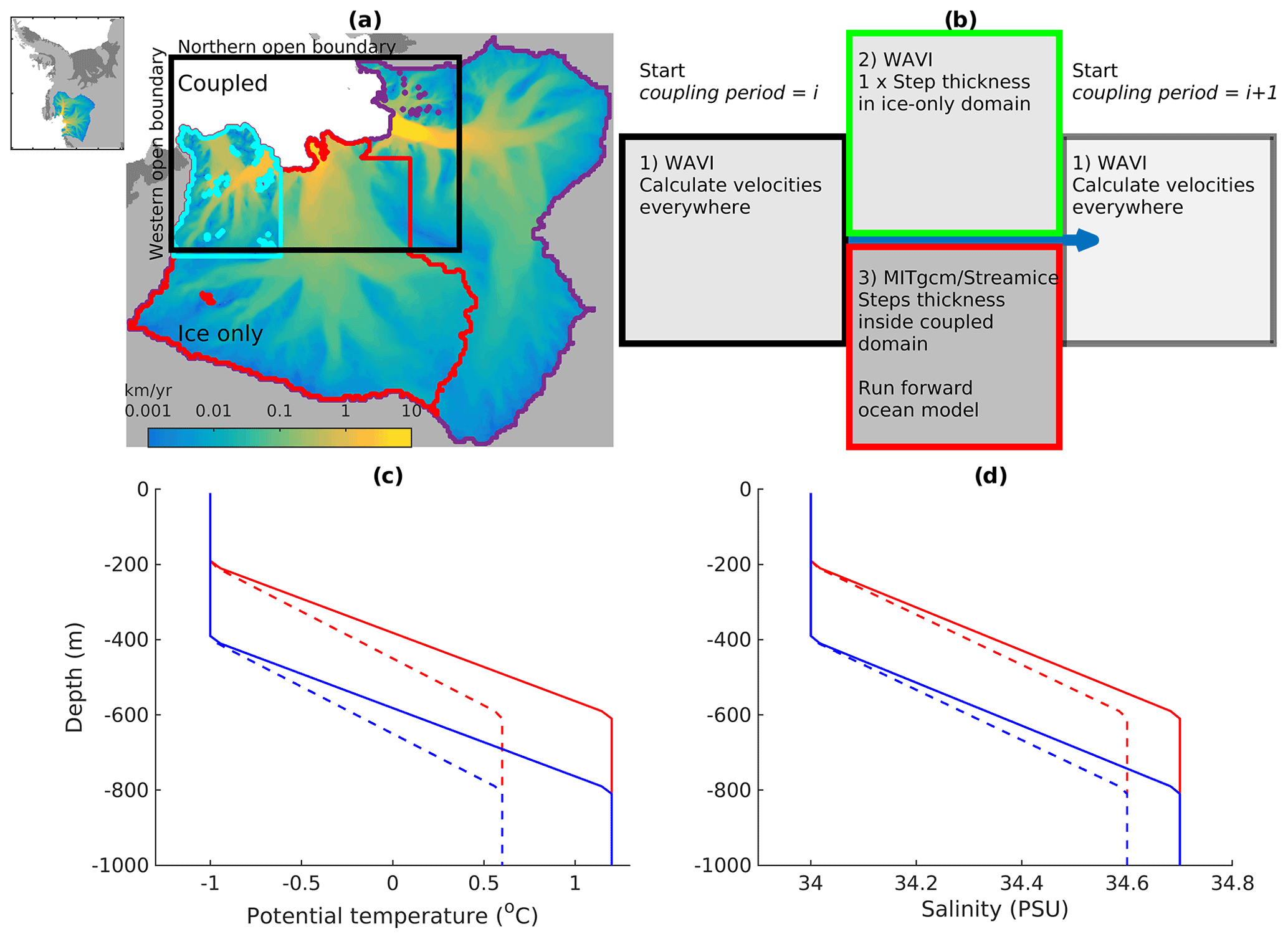
Figure 1(a) Outline of the whole Amundsen Sea sector domain. The black box shows the outline of the coupled domain; the ice-only domain is defined as everywhere outside of this box. The coloured contours represent the three regions used in the analysis: PIG (purple), Thwaites (red) and Smith (cyan). These areas are edited by hand from the Zwally et al. (2012) basins. (b) A schematic diagram of the three grouped steps of the coupled model applied during one coupling period, which are repeated during the coupled simulations. (c) Potential temperature boundary conditions for the northern (solid line) and western (dashed line) boundaries for the warm (red) and cold (blue) cases. Panel (d) as in (c), but for salinity.
2.1 Ice model
In the coupled ice–ocean model, ice velocities are calculated using the Wavelet-based, Adaptive-grid, Vertically Integrated ice sheet model, WAVI (Arthern et al., 2015; Arthern and Williams, 2017). WAVI is a finite-volume ice sheet model including a treatment of both membrane and simplified vertical shear stresses as described by Goldberg (2011). We use a numerical model with a time step of 20 d and a 2 km horizontal resolution covering the whole Amundsen Sea sector domain shown in Fig. 1a. This horizontal resolution has been found to be appropriate in a recent study, currently under review, testing the impact of resolution on grounding-line retreat and SLR contributions, with a nearly identical configuration of the Amundsen Sea sector (Williams et al., 2024). The ice rheology is described using Glen's flow law, with an exponent of n=3. A Weertman sliding law is used (Weertman, 1964), for which basal sliding drag scales with the cube root of sliding velocity, multiplied by a basal sliding drag coefficient C. As described in Arthern et al. (2015), WAVI uses a data assimilation method to match modelled ice velocities and rates of thickness changes with observations of the MEaSUREs 2014/2015 surface velocities (Mouginot et al., 2017a, b) and rate of change of surface elevation from Smith et al. (2020), resulting in an initial state representing conditions in approximately 2015. Partially grounded cells are utilised using a sub-grid parameterisation to better represent the grounding line (e.g. Arthern and Williams, 2017; Pattyn et al., 2006; Cornford et al., 2012; Seroussi et al., 2014), where the grounding fraction is used to proportionally apply the Weertman sliding drag coefficient. An ice model relaxation is then run for a set period of time (4000 years). During this relaxation the grounding line and the thickness of ice shelves remain fixed, but the grounded ice thickness is allowed to change (see Arthern et al., 2015, for full details). This brings the flux divergence into much better agreement with observations of accumulation and rates of ice thickness change but at the cost of the surface elevation and ice velocities agreeing less well with observations (see Appendix A). Ice thickness prior to relaxation and bathymetry fields are from BedMachine V3 (Morlighem et al., 2020; Morlighem, 2022), where a minimum thickness of 50 m is applied to determine the initial ice extent, which includes the current gaps between the east and west of Thwaites Ice Shelf. The ice front and outer catchment boundaries are kept fixed throughout the simulations. Accumulation and englacial temperatures are kept constant in the forward simulations, using data sets from Arthern et al. (2006) and Pattyn (2010), respectively.
2.2 Ocean model
We use the Massachusetts Institute of Technology general circulation model (MITgcm; Marshall et al., 1997) to simulate the ocean circulation in the Amundsen Sea. The model grid uses polar stereographic Cartesian coordinates with horizontal resolution of 2 km and vertical resolution of 20 m, and we use a time step of 200 s. The ocean model domain extent is shown by the black box in Fig. 1a. Note that this does not include the whole continental shelf, so we apply ocean boundary conditions and velocities to the northern and western open boundaries of the domain to impose prescribed Amundsen Sea conditions in idealised “warm” and “cold” experiments. We also examine a third “no melting” case in which no ocean-driven melting is applied to the ice shelves. This study focuses solely on the ice sheet, ice shelf and ocean interactions driven by wider Amundsen Sea conditions, so sea ice and other freshwater sources/sinks are not included in the simulations, and no atmospheric forcing is applied over the model domain.
The boundary conditions in warm and cold experiments are as follows. Following previous studies, an idealised, piecewise linear, vertical profile is applied to replicate the warm CDW layer below cold Winter Water, with a thermocline 400 m thick (De Rydt et al., 2014). The base of the thermocline is placed at 600 m depth in the warm scenario and lowered to 800 m depth in the cold scenario (Fig. 1c, d). These profiles correspond to the warmest and coldest observed Amundsen Sea conditions, in 2009 and 2012, respectively (Dutrieux et al., 2014). On the northern boundary the warm CDW layer has a temperature of 1.2 °C and a salinity of 34.7 (PSU), whereas the western boundary is forced with a more modified CDW layer, with temperature 0.6 °C and salinity 34.6 (PSU) (Fig. 1c, d). In all simulations, at the boundaries, we apply average ocean velocities (1965–2015) from a larger regional model (Holland et al., 2022; Naughten et al., 2022), and we restore sea level to zero.
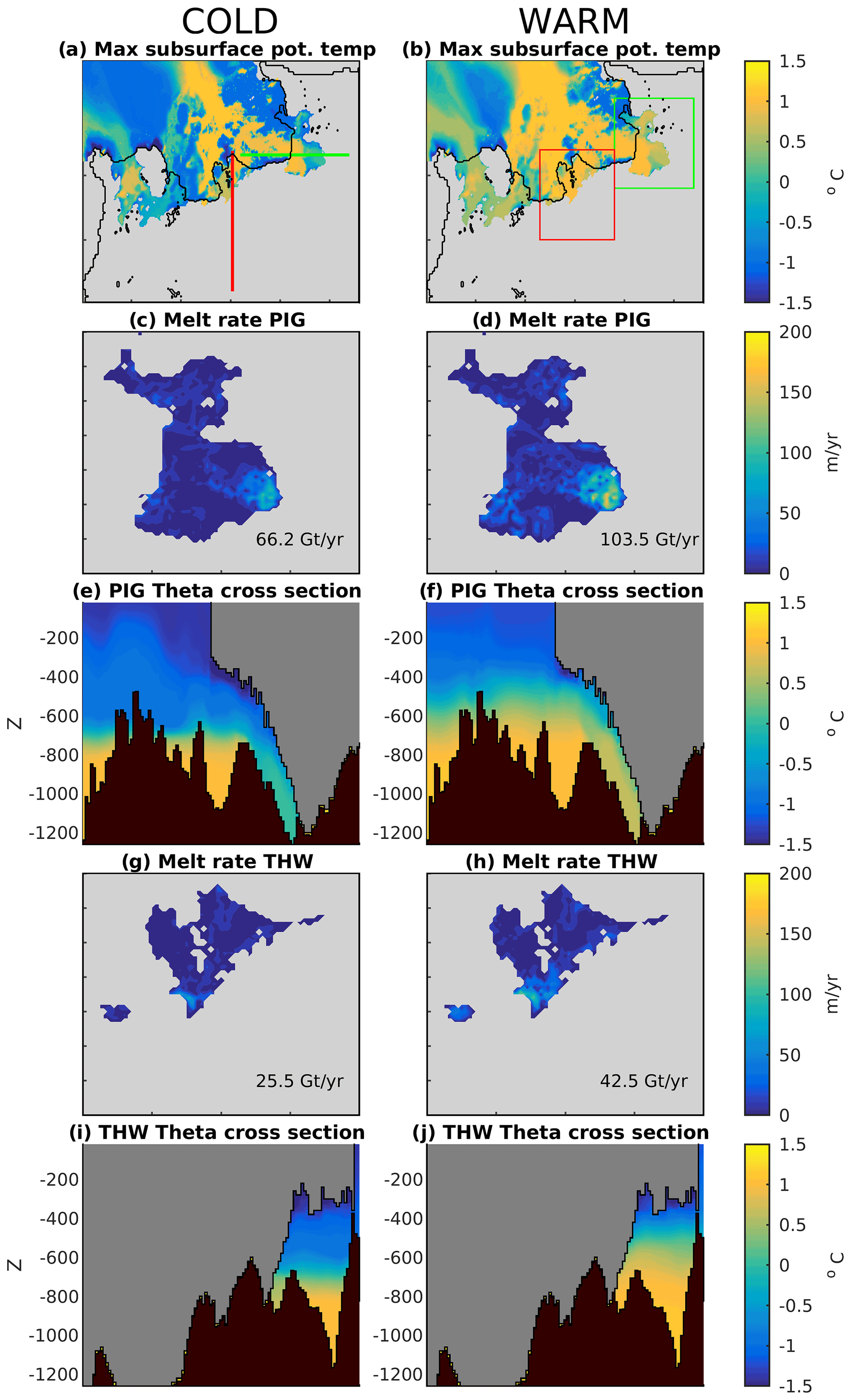
Figure 2(a) Initial maximum subsurface potential temperature over the ice–ocean domain for the cold case. (c) Initial melt rate under PIG Ice Shelf in the cold forcing case over the green box in (b). The label shows the total initial meltwater flux. (e) Cross-section through PIG Ice Shelf taken along the west–east green line in (a) showing initial potential temperature in the cold case. (g) Initial melt rate over Thwaites Ice Shelf in the cold forcing case over the red box in (b). (i) Cross-section through Thwaites Ice Shelf taken along the south–north red line in (a), showing initial potential temperature in the cold case. Panels (b), (d), (f), (h) and (j) as in (a), (c), (e), (g) and (i), respectively, but for the warm forcing case.
Ocean-only simulations, with fixed initial ice geometry, are simulated for 2 years as a spin-up before coupling. The resultant conditions in the ocean model are designed to match the spatial distribution of present-day observed maximum subsurface temperatures over the region (Dutrieux et al., 2014), as shown in Fig. 2a and b. The warm and cold oceanic forcing cases enable different amounts of CDW to reach the base of the present-day Thwaites and Pine Island Glacier (PIG) ice shelves (Fig. 2e, f, i, j). The initial melt rates, after the 2-year ocean-only spin-up, of the Thwaites and PIG ice shelves for the warm and cold simulations are shown in Fig. 2c, d, g and h.
Ice shelf melting is represented by a standard three-equation formulation (Holland and Jenkins, 1999). We tune the dimensionless ice shelf melting drag coefficient in this parameterisation to 0.008. This drag coefficient parameterises the ocean stress on the ice base as a function of the ocean model's mixed layer velocities in order to calculate turbulent ocean heat and salt fluxes for use in the melting calculation (Jenkins et al., 2010). For the PIG and Thwaites ice shelves combined, this value produces the closest average match between the initial MITgcm ice shelf melt rates and those that are implicit in the WAVI initialisation (see Appendix B). This minimises the “coupling shock” – the response of the ice model to any mismatch between these two fields – which occurs when the coupled model simulation commences. Without this calibration, the ice sheet trajectory could be impacted, potentially for many decades (Goldberg and Holland, 2022), by the adjustment of the ice due to the transition from implicit initialised melt rates to arbitrarily different ocean model melt rates at the start of the simulation. Note also that this tuned value is close to a value of 0.01 derived from observations (Jenkins et al., 2010).
BedMachine V3 is used as the basis for the bed and seabed geometry throughout the model. However, we found that without modification this dataset led to rapid grounding and advance of PIG. Closer inspection revealed that the seabed bathymetry may have been underestimated near the grounding line of this glacier in BedMachine V3 (Appendix C). Therefore, throughout the domain we deepen the seabed wherever needed to achieve a minimum water column thickness of 280 m on the staggered Arakawa C-grid's velocity grid points, located on the grid faces, tapering towards grounded ice over 6 km down to a minimum water column thickness of 140 m. This procedure is only applied to cells with no ice basal sliding drag in the initial state and is only done once at the start of the simulation before the WAVI ice sheet model is initialised and relaxed rather than being an ongoing process. This edited bathymetry is used in both MITgcm and WAVI.
2.3 Ice–ocean coupling
This study uses a new, synchronously coupled ice–ocean model, which combines the WAVI ice sheet model with MITgcm. Crucially, this coupling occurs through the MITgcm ice sheet package STREAMICE (Goldberg and Heimbach, 2013), making use of previous synchronous coupling developments (Jordan et al., 2018; Goldberg et al., 2018), which enables the STREAMICE ice thickness to evolve continuously in the ocean model. The basic concept of the new model is that WAVI solves for the ice velocities; MITgcm STREAMICE solves for the ice thickness; and the MITgcm ocean model solves for all ocean properties, including melting and also where the ice thickness evolves. Dividing up computations in this way allows for a fully synchronous coupling because both the ice thickness and ocean properties are solved within MITgcm on the ocean time step. This has two advantages: firstly, the ice thickness and ocean free-surface equations are solved simultaneously, allowing full conservation of mass in the ice and ocean coupled system. Secondly, the melt rate responds instantly to changes in ice thickness.
In principle, this approach is no more expensive than other coupling approaches because the two-dimensional ice thickness equations can be solved on the ocean time step with negligible computational expense compared to that incurred in solving three-dimensional ocean equations. However, the approach does require the MITgcm grid to exist wherever ice may go afloat during the simulation, since grounding-line retreat in MITgcm is accomplished naturally. MITgcm solves the ocean free-surface equation every ocean time step in order to conserve mass, which naturally inflates the water column in the MITgcm ocean model wherever the pressure loading of the ice decreases below floatation (Goldberg et al., 2018). In regions of ice which are not floating, a thin subglacial layer is specified in order to enable the expansion of the ocean column during grounding-line retreat (Goldberg et al., 2018; Jordan et al., 2018). We set it to be 4 m thick, but it could have been set to any relatively small thickness compared to the ocean model vertical resolution. This small value has been previously demonstrated to have no impact on the evolution of the coupled system (Goldberg et al., 2018). This layer, which has no effect on basal sliding drag computed by the ice model, is treated as a porous medium, with Darcy flow used to connect the subglacial cells to each other (Goldberg et al., 2018).
Using an MITgcm domain covering the entire catchment of the Amundsen Sea sector would be very inefficient, since it would include large areas of grounded ice that would never go afloat in the ocean/STREAMICE grid. To avoid this, we introduce the concept of “ice-only” and “coupled” domains (Fig. 1a): in the ice-only domain, WAVI is used to solve for both ice sheet velocities and thickness, while in the coupled domain, WAVI solves for ice velocities and MITgcm solves for ice thickness and ocean properties, as described above. The coupled domain only needs to extend far enough inland to accommodate the grounding-line retreat occurring during a projection, which for this study was determined using test simulations.
The coupled model solution procedure is split into coupling periods, chosen to equal the WAVI time step of 20 d, meaning that the WAVI model state is fixed during each coupling period. Over each coupling period (Fig. 1b) the following takes place: (1) WAVI calculates ice velocities over the whole ice domain for one 20 d time step; (2) WAVI steps forward the ice thickness in the ice-only domain for one 20 d time step; (3) MITgcm receives the ice velocity for the coupled domain and the updated ice thickness on its boundaries and sub-cycles the ice thickness, grounding line and ocean properties within the coupled domain using the 200 s ocean time step for the full 20 d coupling period; and (4) MITgcm passes the new ice thickness and therefore the new ice grounding line for the coupled domain back to WAVI, and the next coupling period commences. Therefore, the choice of the length of the coupling period determines the fastest response time for which the ice velocities can respond to changes in buttressing in the coupled domain, where the ice thickness changes with the ocean time step. The WAVI boundary cells outside of the coupled domain are passed to the MITgcm domain and held fixed while MITgcm runs, and then the thickness throughout the coupled domain is passed from MITgcm to WAVI after each coupling step. This procedure, in addition to WAVI being fixed during each coupling period, keeps the two models'/domains' ice thicknesses from diverging and ensures a smooth transition between the two domains.
For consistency, the same advection scheme that is used in WAVI (Arthern et al., 2015) has been coded into STREAMICE. Ice divergences are updated with the changing ice thickness in STREAMICE every ocean time step, while the ice velocity remains fixed over each coupling period. We adopt the principle that the ocean may only melt ice that has no basal sliding drag applied (Arthern and Williams, 2017), so the WAVI ice basal sliding drag field is passed to MITgcm to decide where melting can occur during each coupling period. This means that no melting can occur on partially grounded cells, as recommend by Seroussi and Morlighem (2018). In addition, this means that if a cell becomes fully ungrounded in MITgcm, ice shelf melting only occurs once the coupling period finishes and a new one starts, which updates the ice thickness in WAVI and subsequently passes back a new basal sliding drag field. However, if, during a coupling period, a grid cell becomes grounded in MITgcm, melting on this cell is immediately switched off. In both the WAVI and STREAMICE models a minimum ice thickness of 50 m is applied.
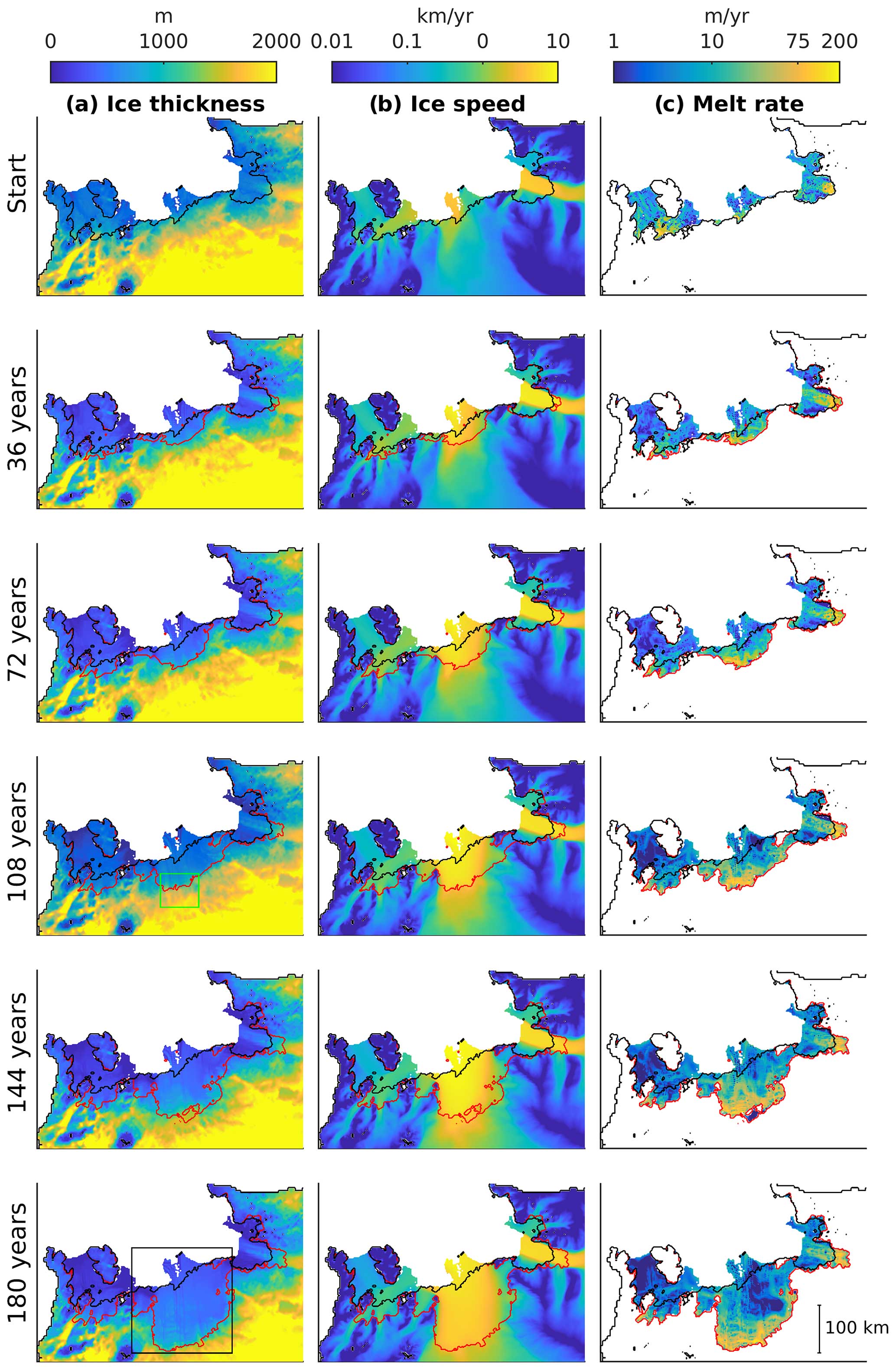
Figure 3Warm forcing case evolution over 180 years. Panels show snapshots of (a) ice thickness, (b) ice speed and (c) melt rates plotted on a logarithmic scale, taken every 36 years throughout the simulation. Initial (black) and final (red) grounding lines are included.
3.1 Simulated evolution of the Amundsen Sea sector
Following initialisation, the coupled ice–ocean model is run forward for 180 years under both forcing cases, as well as a zero-melting case. The evolution of the warm simulation is shown in Fig. 3. The most prominent feature of the simulation is the acceleration (Fig. 3b) and grounding-line retreat of Thwaites Glacier (Fig. 3a). At the start of the simulation, Thwaites Ice Shelf hosts the observed fast-flowing western shelf and slower eastern ice shelf (Fig. 3b), where a pinning point restrains the flow of ice. However, as the simulation progresses, both sides of the ice shelf accelerate, reaching speeds of up to ∼10 km yr−1, but then the whole ice shelf shows signs of deceleration between 144 and 180 years. In addition, Thwaites Glacier experiences substantial grounding-line retreat during this simulation, approximately 130 km of north–south retreat, leading to a reduction in the total mass of grounded ice and the formation of a new, larger ice shelf cavity, which features high melt rates near the grounding line (Fig. 3c). The fixed ice front leads to a large and thin future Thwaites Ice Shelf, which may lead to artificially elevated melting overall, though only low ice shelf melt rates occur on the thinner ice (Fig. 3a, c). However, such trends in ice speed and grounding-line retreat are restricted to Thwaites: neither PIG nor Smith Glacier experiences the same level of acceleration or retreat, although we do observe an initial acceleration of the PIG (which is later reversed) and some grounding-line retreat in both PIG and Smith.
In order to analyse SLR contributions, melting and grounded ice area loss from different regions and to compare the three forcing cases, we divide the domain into three areas: Thwaites, PIG and Smith (Fig. 1a). These areas are edited from the Zwally et al. (2012) basins, where the Smith area has been separated out. In addition, the boundary between the PIG and Thwaites areas is edited by hand to address the otherwise mis-assignment of SLR contributions, melting and grounding ice loss to PIG as Thwaites retreats (Fig. 3). The model projects notable SLR contributions from all three regions, even in the zero-melting case for the Thwaites and Smith areas, which has important implications. This result demonstrates that the initialised ice sheet state in WAVI is intrinsically unsteady and will continue the present-day ice loss for some period of time irrespective of future climatic forcing. This implies that a tipping point may have been passed at some point for this particular initialised ice sheet, likely during the 20th century (Mouginot et al., 2014), and some amount of SLR (at least ∼40 mm in our simulations) is now committed. Zero melting can never occur in the real world because even seawater at the surface freezing point will drive melting at depth due to the pressure decrease in the freezing temperature, so this is a very conservative test of the presence of committed ice change. In the PIG area there is a negative SLR contribution for the zero-melting case (mass gain), though the contribution from PIG is dependent on the particular choice of bathymetry deepening that is implemented (Appendix C). Notably, we observe the largest zero-melting SLR contribution from the Thwaites area, leading to ∼45 mm in 180 years, with a near-constant SLR rate. For the Thwaites area we also obtain some grounding-line retreat, though the rate of loss reduces during the simulation, suggesting that the SLR contribution would stabilise after a further period of simulation.
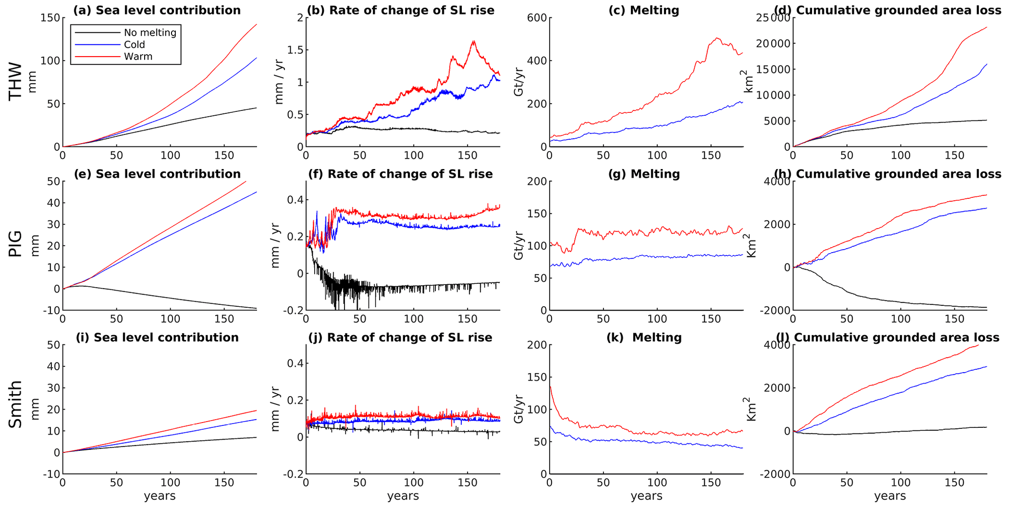
Figure 4Time series shown for the three cases: no melting (black line), cold (blue line) and warm (red line). (a) Cumulative global sea level contribution from the Thwaites area. (b) Rate of change of global sea level contribution for the Thwaites area. (c) Total ice shelf melt rate from the Thwaites area with a 2-year running average applied. (d) Cumulative grounded area loss from the Thwaites area. (e–h) Same as (a–d), but for the PIG area. (i–l) Same as (a–d), but for the Smith area.
The cold and warm cases are far more realistic since they are based on observed Amundsen Sea conditions. Both scenarios contribute much more SLR than the zero-melting case (Fig. 4a, e, i). In both cases, the Thwaites area dominates SLR contributions from the sector, providing approximately two-thirds of the total, and responds differently to melting than the PIG and Smith areas. In the PIG and Smith areas, the rates of SLR with melting are approximately constant but are higher than the rates of SLR in the zero-melting case, increasing to ∼0.3 and ∼0.1 mm yr−1 in the warm case, respectively (Fig. 4f, j). However, in the Thwaites area with melting a trend emerges in the SLR rate (Fig. 4b), increasing from ∼0.2 mm yr−1 at the start of the simulation to ∼1.1 mm yr−1 at the end in the warm case. In addition, we observe rapid jumps in the SLR rate for Thwaites that are not present in the other areas. The increase in the SLR rate in the Thwaites results in an approximately quadratic SLR contribution (Fig. 4a) rather than the more linear SLR contributions obtained for PIG and Smith. In all three areas “noise” is present in the SLR rates due to the instant effects of the changing basal sliding drag field, though this is harder to see for the Thwaites area due to the larger y-axis scale. In addition, we observe an increase in the total melting that occurs from the Thwaites Ice Shelf as the simulation progresses: over the 180 years of the simulation, the total melt flux from Thwaites increases by an order of magnitude, from ∼45 (∼25, respectively) Gt yr−1 at the start of the simulation to over ∼440 (∼210) Gt yr−1 at the end in the warm (cold) case (Fig. 4c), which occurs despite constant oceanic boundary forcings during the simulation. This is explored further in Sect. 3.3. In the PIG and Smith areas, the total melt flux is approximately constant (Fig. 4g, k). However, we do observe a strong correlation between the cumulative integral of melting and the SLR contribution individually for each region (Appendix D). In addition, while the effect of the inclusion is small, we do include ice shelf melting that occurs on ice that has reached the minimum thickness, as while this melting is not allowed to thin the ice further, it still has a partial glaciological effect by stopping the ice from thickening. Furthermore, this melting still has an oceanographic effect in the simulation by cooling and freshening the ocean.
For all regions, we obtain consistently higher SLR rates and grounded ice area loss in the warm forcing case compared to the cold forcing case (Fig. 4b, f, j). However, as a fraction of the total SLR in these models, the difference between warm and cold scenarios is remarkably small, only ∼27 % of total SLR from all regions by the end of the simulations. Given that these scenarios bracket the coldest and warmest ocean conditions on record in the Amundsen Sea, this suggests that the future SLR from this region is only weakly influenced by variations within the observed range of present-day ocean conditions: while melting is important to the SLR, its typical climatic variations are less so. Despite this, in the Thwaites area we observe different timings and strengths in the jumps in the SLR rate between the cold and warm cases (Fig. 4b). We also observe an increasing difference between the cold and warm total melt rates for Thwaites Ice Shelf (Fig. 4c), while for the PIG and Smith areas this difference remains approximately constant (Fig. 4g, k). Additionally, there is a larger relative difference between the melting and no melting cases for the PIG area compared to Thwaites. In the PIG area, ice shelf melting prevents the ice shelf from thickening and re-grounding on the bathymetric ridge below it. In the no melting case, the ice shelf re-grounds on this ridge; the buttressing provided by this re-grounding leads to the large differences between the no melting and melting cases for the PIG area (though this is dependent on bathymetry deepening). While there is a smaller relative difference for the Thwaites area, the presence of melting still has a significant impact, changing the SLR contribution from linearly increasing to quadratic.
Overall, we conclude that melting and SLR have a fundamentally different response in the Thwaites area than the other areas, leading to an increasing SLR rate and total melting rate. In addition, the Thwaites area dominates the SLR contribution for the Amundsen Sea sector over the 180 years simulated. Therefore, the remainder of this study focusses upon the processes underlying this behaviour in the Thwaites area.
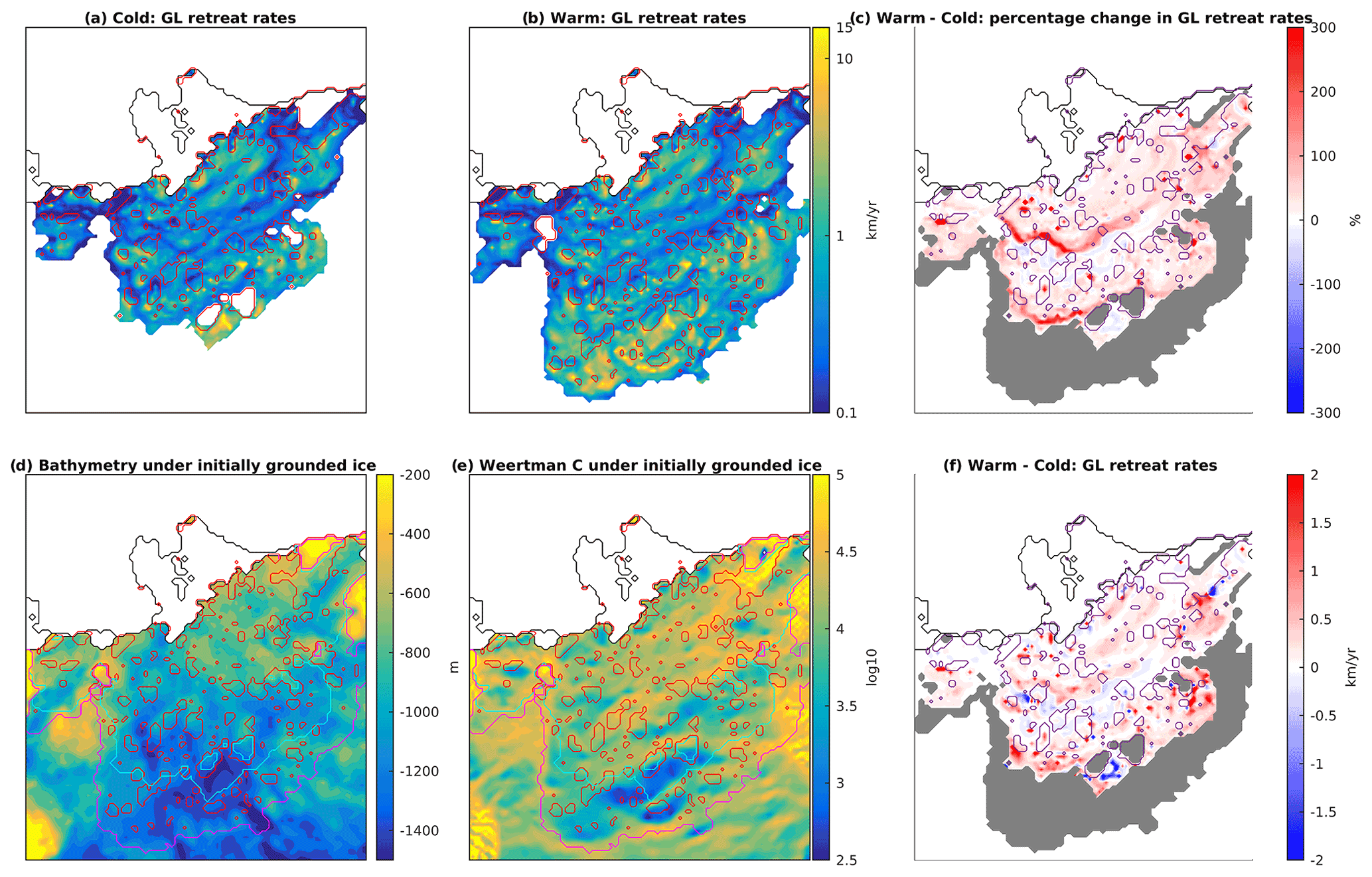
Figure 5(a, b) Grounding-line retreat rates over the 180-year simulations in the cold (a) and warm (b) cases indicated by colours, with colour bar shown in (b). The red contours in (a), (b), (d) and (e) and the purple contours in (c) and (f) show the presence of isolated pinning points during the simulation. (c) Percentage change in grounding-line retreat rates between the cold and warm cases (i.e. the percentage difference between those retreat rates shown in (a) and (b), respectively). Bathymetry (d) and Weertman C coefficient (e) shown under initially grounded ice with final extents of the grounding-line retreat in the warm (magenta) and cold (cyan) cases. (f) The difference in grounding-line retreat rates between the cold and warm cases (colours), as well as final grounding-line area (grey area). The area shown in each panel corresponds to that displayed as a black box in Fig. 3.
3.2 Thwaites Glacier retreat and ice shelf pinning points
Figure 5 shows quantities related to Thwaites grounding-line retreat, which is one of the key features that differentiates this area from the PIG and Smith areas. Over the simulation, the warm case has a larger area of grounding-line retreat than the cold case, with a faster rate on average (Fig. 5a, b, c, f). Grounding-line retreat rates are calculated from the discrete migration of the grounding line across grid cells. Specifically, the retreat rate in each grid cell is calculated as , where ΔtGL is the time between when the subject cell first becomes a grounding-line cell (any of the eight adjacent cells are floating) to when that cell ungrounds, and ΔxGL is the grid cell width or diagonal extent depending on which adjacent cell was first floating. Figure 5d and e show the bed depth and “Weertman C” drag coefficient over the ice area that is initially grounded. A lower Weertman coefficient corresponds to a more slippery bed. In addition, the bathymetry in this area generally deepens inland, which could promote grounding-line retreat (Weertman, 1974; Schoof, 2007). In both warm and cold cases, highly heterogeneous retreat rates are observed (Fig. 5a, b), with areas of fast retreat as high as ∼10 km yr−1 in proximity to areas of much slower retreat. Towards the end of the warm case simulation, the grounding line experiences rapid retreat (Fig. 5b) across a deep and slippery bed section (Fig. 5d–e) before slowing down as it encounters a ridge of shallower and less slippery bed (Fig. 5d–e), where it remains until the end of the simulation. These features explain the large variations in the Thwaites area SLR rate in the last ∼50 years of the simulation (Fig. 4b). In particular, the retreat onto the shallower and less slippery ridge at the end of the warm simulation decreases the ice flux across the grounding line and corresponds with the Thwaites region's decreasing SLR rate during the last 25 years of the simulation.
Comparing the cold and warm scenarios we see the effect of increased melting on grounding-line retreat rates. More specifically, we observe areas of elevated grounding-line retreat rate in the northern part of the ungrounding area, below which is an area with minimal sensitivity to melting scenario, and again increased rates in the south (Fig. 5f). There are very large percentage increases in grounding-line retreat rates in two clear bands on the retreated area (Fig. 5c), where two bands of slow retreat rates in the cold case are not present in the warm case.
In addition, we observe the formation of many pinning points as Thwaites Glacier retreats, shown by red and purple contours in Fig. 5 for the different cases. An ice grid cell is flagged as a “pinning point” if it is grounded but separated from the main grounded ice sheet by floating ice. The red and purple contour is then drawn around all cells that are flagged as pinning points in any one of the outputs. The pinning points are generally located on areas of shallower bathymetry that are downstream of areas of deeper bathymetry (Fig. 5d). The pinning points typically feature slower retreat rates, and inshore of these pinning points we generally observe areas of faster retreat (Fig. 5a, b). These pinning points are crucial for the future evolution of Thwaites Glacier, as they provide drag and buttressing as the ice retreats. The importance of these pinning points is determined by their size, position and duration, so we examine these features and their relationship to SLR rates from the Thwaites area.
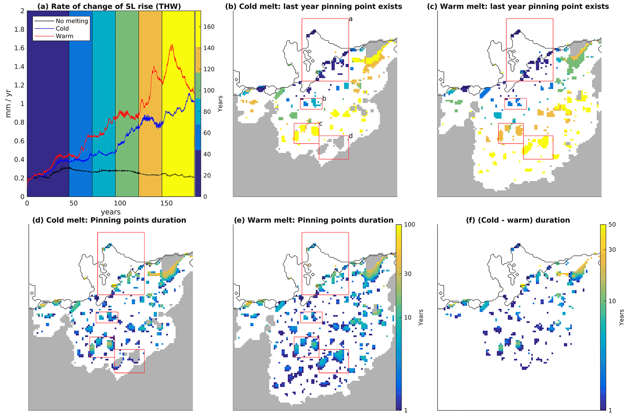
Figure 6(a) SLR contribution rates for the Thwaites area for warm (red), cold (blue) and no melting (black) cases. The background colour indicates the time in the simulation according to bands of 25 years with a longer starting (ending) band of 45 (35) years. (b) Colours indicate the band of the final year that pinning point cells exist for the cold melt case, according to the colours shown in (a). Note that only pinning points that exist for over 1 year are shown. Red labelled boxes refer to groups of pinning points discussed in the text. (c) Same as (b), but for the warm case. (d, e) Pinning point duration, taken as the time from isolation to ungrounding, for cold (d) and warm (e) cases. (f) Difference in pinning point duration between cold and warm cases (i.e. the difference of the data shown in d and e) where pinning point locations match. In (b)–(e), grey regions indicate areas which do not become ungrounded during the simulation. The area shown in panels (b)–(f) is shown with a black box in Fig. 3.
Figure 6b–c show the ungrounding time of pinning points in the cold and warm cases, respectively. By examining these times, we can compare how the ungrounding of pinning points relates to jumps in SLR rate that we observe from the Thwaites area. The labelled red boxes in Fig. 6b show the key groups of pinning points in the simulations.
Within the first 60 years, the SLR rates of the warm and cold forcing cases diverge (Fig. 6a). In the warm case, pinning point group “a” completely ungrounds between years 25 and 60 (Fig. 6c), with the final ungrounding of the last pinning point in group “a” coinciding with the ungrounding of group “b”. The removal of the combined associate buttressing leads to a large jump in SLR rate in the warm simulation at ∼60 years. However, in the cold simulation, some of these pinning points in group “a” remain grounded until beyond 95 years (Fig. 6b), leading to a period of relatively steady SLR rate in this simulation (Fig. 6a). In the zero-melting case, part of pinning point group “a” and all of “b” remain grounded throughout the simulation (not shown), and SLR rates remain approximately constant as a result (Fig. 6a). In the warm simulation, group “c” becomes ungrounded by ∼130 years, causing a rapid increase in SLR rate, and the loss of group “d” at ∼145 years leads to another large jump. The cold simulation loses group “c” at ∼170 years, leading to a small jump in SLR rate, while group “d” remains grounded at the end of the simulation.
Figure 6d–e show the duration of the pinning points – the time between separation from the main body of grounded ice to ungrounding. There is a large variation in pinning point durations, with some lasting less than a year, while others persist for decades. In general, the duration of pinning points is lower in the warm case (Fig. 6d–f), with an average pinning point duration of ∼6 years over matching pinning locations, compared to ∼10 years in the cold case, leading to the different ungrounding timings and SLR rates as described above. Reducing the duration of pinning points increases the intensity of periods of rapid ice acceleration and grounding-line retreat, leading to the differences in the spatial map of grounding-line retreat rates between the cold and warm cases shown in Fig. 5c and f.
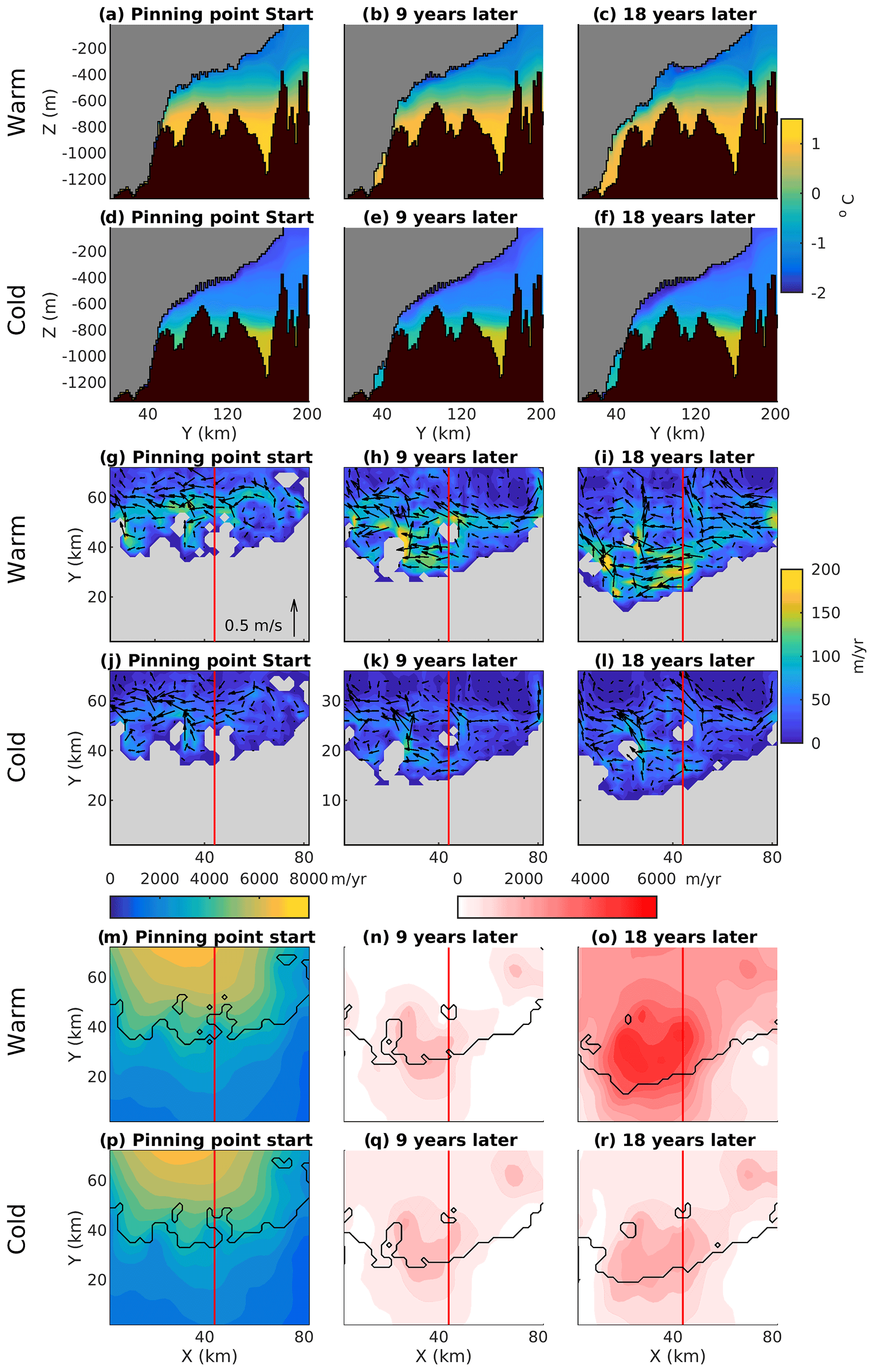
Figure 7Evolution of conditions as grounding line retreats over pinning points. Snapshots every 9 years starting from the date of group “c” pinning point formation in the warm and cold cases (118 and 144 years, respectively). (a–c) Cross-section through the Thwaites Ice Shelf, taken along the red line in (g) extended to ice front for the warm case. (d–f) Same as (a–c), but for the cold case. (g–i) Melt rates for the warm case, with arrows showing ice shelf boundary layer ocean velocities. (j–l) Same as (g–i), but for the cold case. (m) Ice speed snapshots at start of pinning point formation, and (n) and (o) show differences for the warm case. (p–r) Same as (m–o), but for the cold case. Area shown in (i)–(x) is shown in Fig. 3 as a small green box.
To illustrate the key role of pinning points, we now focus on the ungrounding of group “c”, which causes the rapid jump in SLR rate at year 130 in the warm simulation and the smaller jump at year 170 in the cold simulation. Figure 7 shows the evolution of the two simulations, starting from the individual dates of formation of the group “c” pinning points. Figure 7a–l show the ice geometry and ocean conditions throughout the subsequent evolution. To begin with, the grounding line is located in shallower bathymetry at the top of a retrograde slope (Fig. 7a, d). Ungrounding then occurs laterally around this point, including upstream, encircling the pinning point and leaving it isolated from the rest of the grounded ice (Fig. 7h, k). Note that the pinning point is grounded on the side of the shallower bathymetry rather than on top of the bathymetric feature. With the grounding line now in a deeper bed an acceleration is expected, although the pinning point continues to provide basal sliding drag that resists the flow. The advection of thicker ice from the deeper bed upstream enables the ice to remain grounded on the shallower bed beneath the pinning point. Therefore, only a small acceleration is observed at 9 years, while the ice remains grounded on the pinning point (Fig. 7m–r).
However, melting now occurs in the newly opened cavity upstream of the pinning point. This thins the ice, enlarging this cavity, enabling greater oceanic connection, and leading to higher ocean velocities and melt rates (Fig. 7h, k). This melting and thinning feedback eventually leads to sufficient thinning upstream of the pinning point for it to unground completely (Fig. 7i). The resulting loss in buttressing leads to a large increase in ice speed (Fig. 7o), further rapid grounding-line retreat and a jump in SLR rate. Therefore, the distribution and strength of localised melt rate patterns strongly determine the duration of these pinning points and thus the overall ice retreat. This is shown clearly in Fig. 7g–l, with the warm case leading to higher melt rates and a much faster ungrounding of the pinning point. The melt rates around these pinning points are highly heterogeneous (Fig. 7g–l), with elevated melt rates typically occurring on their eastern side, where rapid ocean currents drive high melt rates. These rapid currents occur where buoyancy-driven meltwater flow is trapped against the grounding line by Coriolis force (Holland and Feltham, 2006).
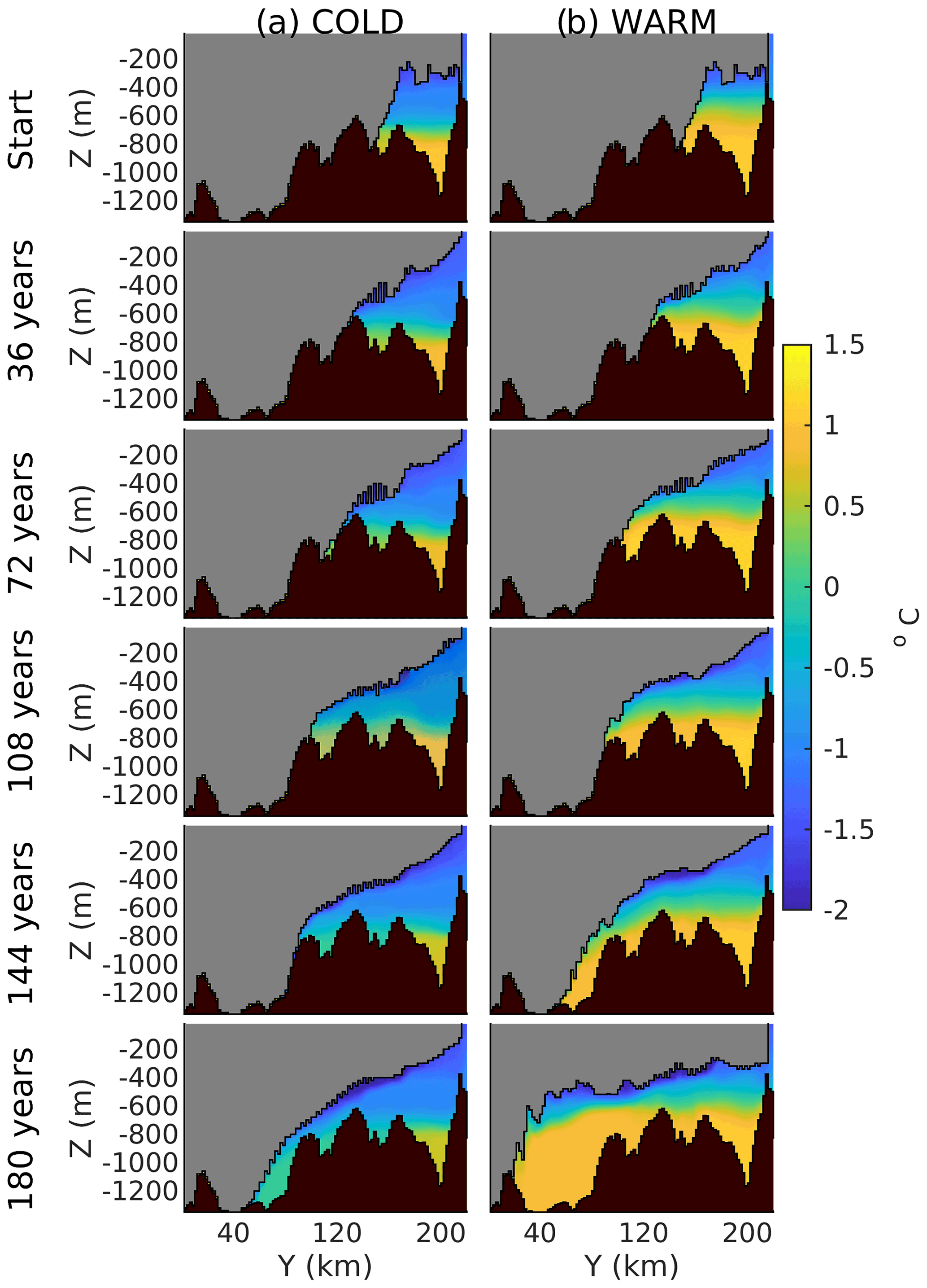
Figure 8Cross-sections of potential temperature beneath Thwaites Ice Shelf for cold (a) and warm (b) cases, taken every 36 years, along the same section as shown in Figs. 7 and 2i and j, which is represented in Fig. 2a as the red line.
3.3 Thwaites Ice Shelf geometric melting trends
An increasing trend in the total ice shelf melting occurs over the evolving Thwaites Ice Shelf during both the warm and cold forcing simulations (Fig. 4c). The wider oceanic forcings are fixed, so these trends must be driven by geometric changes in the ice shelf cavity. In Fig. 8 we show how the Thwaites cavity geometry and ocean conditions evolve in the two cases. The warm case has a higher thermocline, so the warm CDW is more easily able to flow over ridges and flood the new cavity areas. In the cold case, the access of the warmest CDW is blocked by seabed highs, with only more heavily modified CDW reaching the ice base. However, sufficiently warm water is still able to drive melting close to the grounding line. In both cases the ice base near the grounding line remains steeply sloped throughout the retreat.
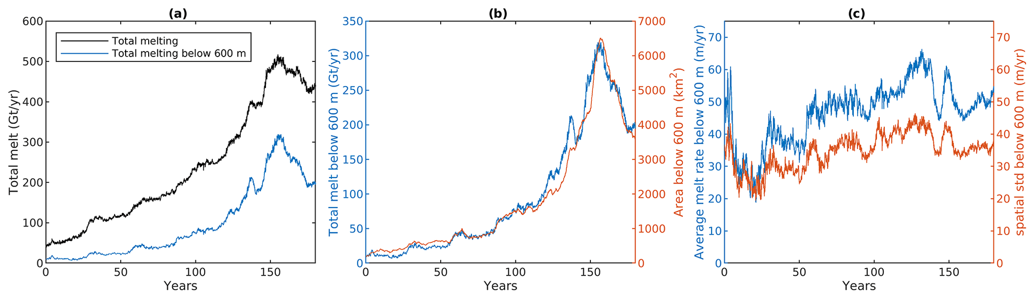
Figure 9(a) Total melt flux from the full Thwaites Ice Shelf area (black) and from grid cells located below 600 m depth only (blue). (b) Total melt flux from grid cells below 600 m and total ice area below 600 m. (c) Average melt rate on grid cells located below 600 m depth and spatial standard deviation of these melt rate values.
Figure 9a shows the evolution of total melt flux from the Thwaites Ice Shelf in the warm case for both the entire ice shelf and for ice below 600 m depth only, which is the thermocline depth in this case. For the majority of the simulation, the total melt flux from the entire ice shelf increases, but it decreases during the last 25 years. Most of the trend in ice shelf melting occurs in the deeper ice, with melting below 600 m peaking at an increase of ∼30 times its initial value, which suggests that as the grounding line retreats, an increase in ice shelf base area below the thermocline controls total melting (Fig. 9b). This confirms that the trend in melting does not result from the increasing ice shelf area associated with an artificially fixed ice front. The increase in deep ice area occurs because the groundling line retreats into deeper bathymetry but also because the slope of the ice shelf base, below 600 m, gets shallower during the simulation, as shown for example in Fig. 8. Without an increasing trend in melt flux, the thicker ice advected across the grounding line as the ice sheet retreats into deeper bathymetry would result in re-grounding on pinning points further downstream. However, towards the end of the simulation the groundling line retreats slowly onto a shallower ridge (Fig. 5d), where the shallowing grounding-line depth decreases the ice shelf area below 600 m and subsequently decreases the total amount of melting below 600 m. The close correspondence in the increase between total melting (10 to 197 Gt yr−1) and ice base area (180 to 3560 km2) implies that the average melt rate (m yr−1) beneath deep ice below 600 m is approximately constant at ∼45 m yr−1 (Fig. 9c). However, we do find some temporal variability in this average melt rate, with it varying up to 50 %, and importantly the local melt rates are highly spatially variable, with a spatial standard deviation close to the mean value. This spatial variability is important for the effect of melting on small-scale pinning points, as described above.
This study considers the future evolution of ice streams in the Amundsen Sea sector using a coupled ice–ocean model. Under both warm and cold forcing we find large grounding-line retreat and ice acceleration from Thwaites Glacier, with the Thwaites area dominating future SLR contributions from the region. The SLR from the Thwaites area is consistent with a previous coupled model study (Seroussi et al., 2017), which considered a shorter time span of 50 years. In this study however, we show a larger sensitivity to a realistic range of ocean forcings, in the shorter and longer term, and an increasing SLR rate, which continues over the first 160 years, from the Thwaites area. This was not observed in previous coupled modelling of Thwaites Glacier (Seroussi et al., 2017), although it was observed in some ice-only simulations, depending on uncertainty in ice dynamics (Nias et al., 2019) and uncertainty in melt rates (Arthern and Williams, 2017). A previous ice-only study has set 1 mm yr−1 SLR rate to be the threshold that implies rapid retreat and collapse of Thwaites Glacier (Joughin et al., 2014), and this is exceeded sooner in our simulations, within 125 years, than in the simulations of this previous study. However, our simulations are not long enough to see how the full implications play out over multiple centuries.
The SLR contributions in this study of 70–89 mm after 100 years for the Amundsen Sea sector are within the uncertainties of previous ensemble studies (Nias et al., 2019; Edwards et al., 2021). However, the SLR and stability suggestions in this study do differ from recent studies, which found that the present-day geometry is not inherently unstable when starting from a stable starting position (Hill et al., 2023) and that the Amundsen Sea sector has not tipped yet (Reese et al., 2023). We suggest that these differences arise primarily through the different ice sheet model initialisation strategies adopted, which variously use a spin-up period (Reese et al., 2023), data assimilation of ice velocities into a steady state (Hill et al., 2023), or assimilation of ice velocities and observations of unsteady thinning (present study). Also, the date of initialisation and differences in resolutions, datasets used and model physics may also play an important role. Larger coupled model ensembles are needed to assess these aspects. Without these model ensembles there is high uncertainty, for example, in SLR contributions and the timing of when pinning points become ungrounded. This study is designed to provide a small number of physically advanced coupled simulations focusing on ice–ocean processes rather than providing a larger but uncoupled set of predictions of future SLR contributions from the region.
In our simulations, the increase in SLR rate from the Thwaites area is caused by ocean-driven melting, and the magnitude of this increase is sensitive to different rates of melting in warm and cold scenarios. The SLR rate is governed by a balance between retreat of the grounding line into deeper bed regions and the formation and duration of pinning points during this retreat. Crucially, this study shows the importance of ocean-driven melting in ungrounding these pinning points, reducing ice shelf buttressing and enhancing grounding-line retreat. It should be noted that the modelled rates of ungrounding upstream of pinning points are high enough to explain recent observations of grounding-line retreat rates (Graham et al., 2022). Other studies have hypothesised about the mechanics and importance of pinning points (Thomas, 1979) and have shown the effect of pinning points in an idealised ice–ocean coupled model (De Rydt and Gudmundsson, 2016). In this study we clearly show the importance of these mechanisms in a synchronous coupled model of the future Thwaites Ice Shelf, with strong spatial variability in ice shelf melting determining the duration of these pinning points and therefore their influence on SLR. Our use of a synchronously coupled model means variations in the ice thickness are instantly felt in the ocean model's melting calculation. This could impact the speed of the evolution of these pinning points, though further work is required to determine the impact of this coupling on the ice dynamics. The importance of future pinning points suggests the need for more accurate knowledge of bathymetry and bed properties in the grounded portion of Thwaites Glacier, as well as highlights the importance of accurately modelling the effects of pinning points in both ice sheet and ocean models. We have shown that high-resolution coupled ice–ocean models are required to investigate the effect of pinning points on ice dynamics, as these small features need to be resolved in the ice model, and the strong spatial variability in ice shelf melting around them needs to be recreated.
One important question raised by our study is why Thwaites Glacier appears to behave differently from the other glaciers in the region. We speculate that this is caused by the wide trunk of this glacier. As the grounding line of the Thwaites Glacier retreats it forms an extremely short and wide ice shelf, unlike the other glaciers in the region, whose ice shelves are confined within embayments. As a result, the buttressing provided by lateral ice shelf margins is very weak for Thwaites Glacier; this also explains the high sensitivity to pinning points which therefore provide the majority of the buttressing of Thwaites. Therefore, while a recent study found that Thwaites Ice Shelf provides limited buttressing in the present day (Gudmundsson et al., 2023), we find that future configurations of Thwaites Ice Shelf will provide important buttressing, via future pinning points, as its groundling line retreats. The dependence of this future buttressing on ocean forcings will determine the future SLR from this sector.
The simulations show how the geometric changes in the Thwaites Ice Shelf and its cavity can lead to an increasing ice area being exposed to deep warm waters, leading to an increasing trend in total melt flux. Although this general depth dependence on melting is often captured by parameterisations of melting (Asay-Davis et al., 2017), we have shown that there is strong spatial variability in melting, and this spatial variability has important consequences for pinning point duration. Therefore, as parameterisations of basal melting generally lack a strong physical basis and perform poorly in spatial detail (Burgard et al., 2022), they may be expected to struggle to capture this spatial variability, affecting the evolution of these pinning points and the resultant SLR contribution rate from Thwaites. However, future work is required, running sets of ice-only simulations, to perform an extensive comparison of the wide range of basal melt rate parameterisations. Observations of ice shelf melt rates around such features with sufficient spatial coverage are currently lacking but are essential for improving future modelling efforts. The increasing trend in total melt rates is needed to maintain the ice retreat, as it counteracts increased ice thickness advection across the grounding line, which would otherwise ground the ice on bathymetry further downstream.
One of the limitations of this study is that steady, idealised, ocean forcings are applied to the northern and western boundaries. However, ocean conditions in the region are known to have strong decadal variability (Jenkins et al., 2018; Dutrieux et al., 2014). Some of the pinning points only exist for ∼10 years, so decadal variability in oceanic forcings may have an important role in how quickly these pinning points are ungrounded. In addition, a superimposed anthropogenic warming trend in ocean forcing may be expected in the Amundsen Sea (Holland et al., 2022; Naughten et al., 2022), which could decrease the duration of future pinning points and speed up the retreat of Thwaites Glacier. However, while the forcings used in this study are idealised, they are based on the best available information of present-day extremes in observations (Dutrieux et al., 2014). These forcings also agree approximately with the time average of recent projections of future warming in the region (Naughten et al., 2023), which found linearly rising trends of ocean temperature in all tested climatic scenarios. The steady warm and cold forcings used in this study have an average temperature between 200–700 m depth of ∼0.35 and °C, respectively. The warm case approximates the time-averaged temperatures at this depth over the similar trends projected in 100-year simulations of the Paris 1.5 °C, Paris 2 °C and RCP 4.5 climatic conditions (Naughten et al., 2023), while the cold case approximates a cold historical state (Naughten et al., 2023). Another limitation of this study is the use of an ocean model that does not represent the evolution of oceanic conditions and sea ice on the wider Amundsen Sea continental shelf. As such, our model might lack important feedbacks such as increased ocean currents driven by ice shelf meltwater bringing more CDW onto the shelf and driving higher melt rates (Kimura et al., 2017; Jourdain et al., 2017; Donat-Magnin et al., 2017). With an order-of-magnitude increase in ice shelf melting in our projections, such feedbacks would be substantial. In addition, the ocean simulation lacks the physical presence and effect of some freshwater sources, like sea ice and icebergs, which impact the stratification of the water column, oceanic currents and the delivery of warm CDW to the base of ice shelves in the region (Bett et al., 2020). The lack of sea ice in particular could increase the heat content of CDW reaching the ice shelf bases due to the lack of sea-ice-driven convective processes cooling the CDW layer (St-Laurent et al., 2015; Webber et al., 2017). However, it remains unknown how this cooling influence might vary over the coming centuries. These simulations additionally lack subglacial freshwater discharge, which at the grounding line has been found to increase ice shelf melting locally in previous ocean modelling studies (Nakayama et al., 2021), but overall, its effect is small in this region (Holland et al., 2023).
A key limitation of the model used in this study is the lack of calving-front retreat, which could impact ice dynamics, ocean conditions and total melting (e.g. Bradley et al., 2022; Joughin et al., 2021). As well as using a fixed temperature field, the model lacks an evolving damage field (Lhermitte et al., 2020). Therefore, the model may be sensitive to the time of initialisation, as this will determine the level of the damage that is applied for the entire forward simulation. However, we believe that these limitations cause our simulations to be a conservative estimate of Thwaites Glacier retreat for the cold and warm cases, as calving and evolving damage are only expected to enhance the retreat. Barring the existence of major calving- or damage-driven ice retreat over the next 180 years, our results suggest that the ocean-driven ungrounding of pinning points will dictate the future SLR from the Amundsen Sea sector. However, strong sensitivity of ice sheet projections to basal friction laws provides uncertainty to modelled ice retreat rates and mass loss, with the Weertman sliding law used in this study found to systematically predict the lowest ice mass losses (Brondex et al., 2019; Cornford et al., 2020). It should also be noted that uncertainties in the accumulation field could potentially affect the modelled ice dynamics, including modelled SLR and grounding-line retreat rates. In addition, the accumulation field used in this study is held steady, and therefore any effects of future trends in this field are omitted, which could mitigate ocean-driven ice loss to some extent (Edwards et al., 2021). Thus, this study focusses solely on dynamical ice loss driven by ocean melting.
All these ice dynamical limitations affect the no melting case results in this study. However, some of these limitations lead to specific additional caveats to the no melting case, where they may have the greatest impact. For example, the fixed ice front mask includes the current gaps between the east and west of Thwaites Ice Shelf, and these gaps cannot recover during the simulation. In the no melting case, where the ice shelf thickens and recovery of this damage should be possible, this could lead to an overestimation of SLR contributions from this hypothetical case.
This study presents, for the first time, 180 years of ice evolution in the Amundsen Sea sector of the West Antarctic Ice Sheet using a new synchronously coupled ice–ocean model, which includes full mass conservation in the coupled ice–ocean system and an instantaneous response of melt rates to the evolving ice geometry. The coupled simulations were forced with idealised warm and cold ocean conditions in the wider Amundsen Sea and compared to each other, as well as to a zero ice shelf melting case.
Even in the zero-melting case, the model predicts that the Thwaites and Smith areas lose ice mass during the simulations. This implies that the ice sheet model is initialised into an intrinsically unsteady state so that in these simulations a tipping point may have occurred in the past and we are now committed to further sea level rise from this sector. However, when melting is activated in the coupled model, the rates of ice loss are much higher. This implies that ocean melting plays an important role in the future SLR contribution from this sector, though the difference between warm and cold scenarios is relatively modest at only ∼27 % of the total SLR.
For Pine Island and Smith glaciers, the rate of SLR remains relatively constant at approximately 0.3 and 0.1 mm yr−1, respectively, throughout the projections, leading to a linearly increasing sea level contribution. The Thwaites Glacier area provides a much larger sea level contribution and features an increasing SLR rate, which causes its sea level contribution to increase approximately quadratically with time. The rate of SLR from Thwaites Glacier is closely controlled by the formation and duration of isolated pinning points during the retreat of its grounding line. Ocean-driven melting is crucial in driving the ungrounding of these pinning points by thinning the ice upstream, and this is the key mechanism by which future ocean conditions affect the SLR from this sector.
The coupled simulations show a large geometry-induced increase in total ocean-driven melting as Thwaites Glacier retreats and its ice shelf enlarges. This increased melting counteracts ice shelf thickening associated with thicker ice being advected across the deeper grounding line, which would otherwise cause the ice to ground downstream and arrest the retreat. Our simulations indicate large spatial and temporal variability in the melt rates at depths below 600 m. This variability will not appear within simple melting parameterisations.
Our results also suggest that accurate modelling of ocean-driven melting and ice response around pinning points and accurate characterisation of the bed geometry and properties that lead to the formation of pinning points must be future research priorities. In addition, the further development and application of coupled ice–ocean models must be a priority, as it is difficult to envision how many of these results could have been achieved with parameterised ocean-driven melting, though further work is required to symmetrically compare the ice–ocean coupled model to the wide selection of melting parameterisations.
The relaxation step that is applied to the ice model brings the rates of elevation change into much better agreement with observations whilst resulting in only relatively small differences in the ice surface speed (Fig. A1 e, f) and grounded ice thickness (Fig. A1 b, c) compared to observations.
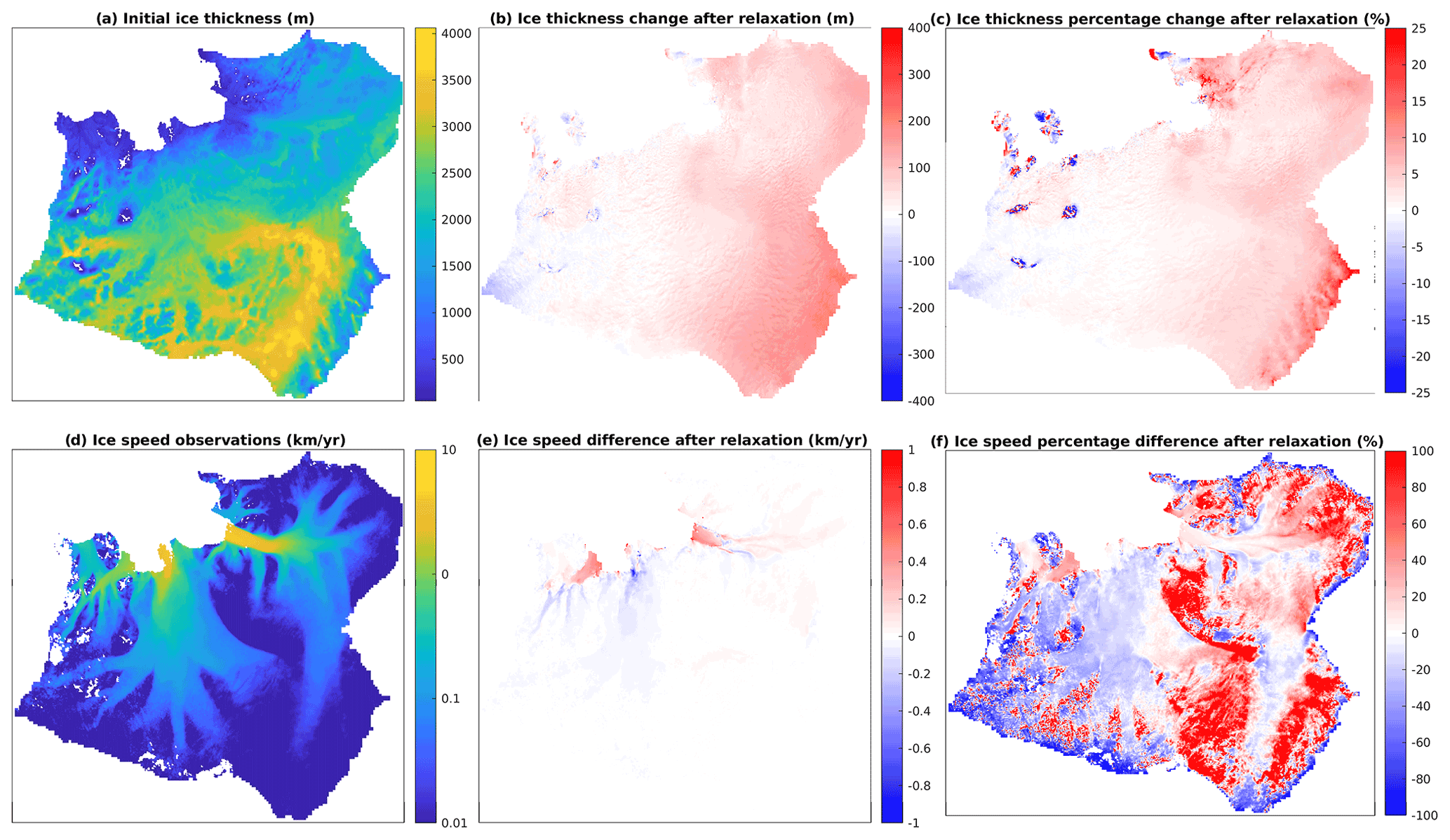
Figure A1(a) Initial ice thickness from the BedMachine V3 dataset (Morlighem et al., 2020; Morlighem, 2022) before relaxation. (b) Changes in ice thickness from relaxation step. (c) Percentage changes in ice thickness after relaxation step. (d) Surface ice speed from MEaSUREs 2014/2015 (Mouginot et al., 2017a, b). (e) Model ice speed difference to observations after the relaxation step. (f) Model ice speed percentage difference to observations after the relaxation step. All plots shown for the full ice domain.
In the initial setup of the ice model, we can calculate the implicit melt rate (IMR), which is the melt rate required to recreate observed present-day surface elevation changes in the ice model, given initial ice model velocities and geometry (Arthern and Williams, 2017). In this model, we attempt to minimise initial coupling shock by reducing the mismatch between the ice model IMR and the initial ice shelf melting field calculated from the MITgcm ocean model. To do so, we tune the dimensionless ice shelf melting drag coefficient in the three-equation formulation of melting parameterisation used in MITgcm (Jenkins et al., 2010). We found that a choice of drag coefficient of 0.008 minimises the combined PIG and Thwaites ice shelve mismatch in total melt flux (Fig. B1), while average ocean forcings are applied with the thermocline placed at 700 m depth.
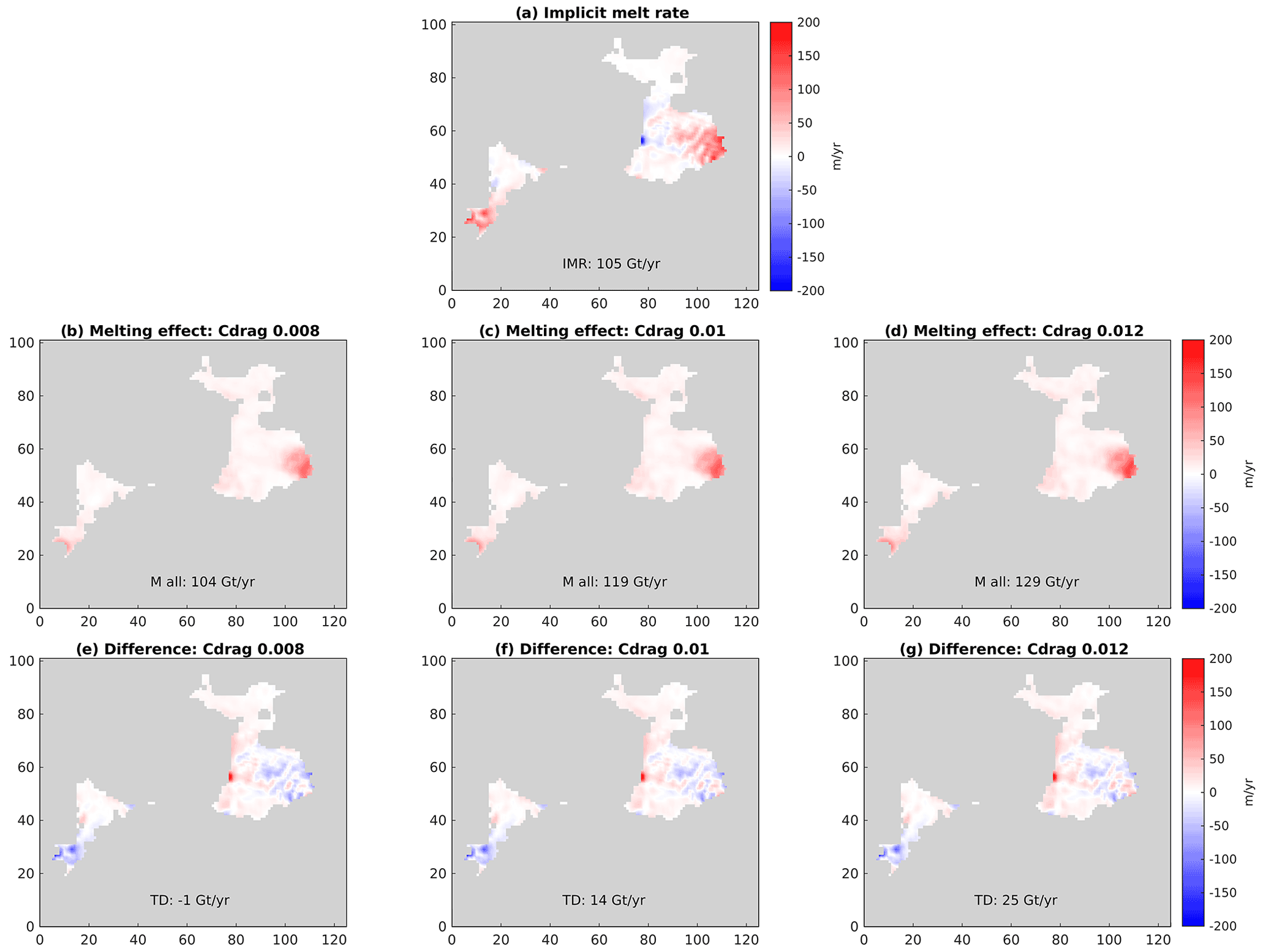
Figure B1Area shown for the PIG and Thwaites ice shelves. (a) Initial implicit melt rate from the WAVI ice sheet model. (b) Initial ice shelf melt rate from MITgcm for different values of the ice shelf melting drag coefficient as follows (and labelled): 0.008 (b), 0.01 (c) and 0.012 (d). (e–g) Difference between initial implicit melt rate and initial ice shelf melting for MITgcm melt rates shown in panels (e)–(g).
To ensure the bathymetry field from BedMachine V3 (Morlighem et al., 2020; Morlighem, 2022) has a specified minimum water column thickness under the initially floating ice area on the staggered Arakawa C-grid's velocity grid points, located on grid faces, we performed a “deepening” procedure, in which the bathymetry in areas with a water column thinner than a specific value is artificially deepened. This procedure was applied only to grid cells in which no ice basal sliding drag is applied in the initial state and occurs only once in a simulation before the WAVI ice sheet model is initialised and then relaxed. This is because the bathymetry in ice shelf cavities is poorly known, while beneath the grounded ice sheet the bed is better known from radar soundings. We found this step is necessary because, without it, the initial PIG Ice Shelf cavity has an excessively thin water column near the grounding line. This leads to minimal ice shelf melting in this region (Fig. C1c), which leads to a large mismatch with the calculated initial IMR (Fig. B1). This, combined with the shallow bathymetry, leads PIG to re-ground immediately at the start of the simulation, resulting in unrealistically low SLR rates from this region (Fig. C1d).
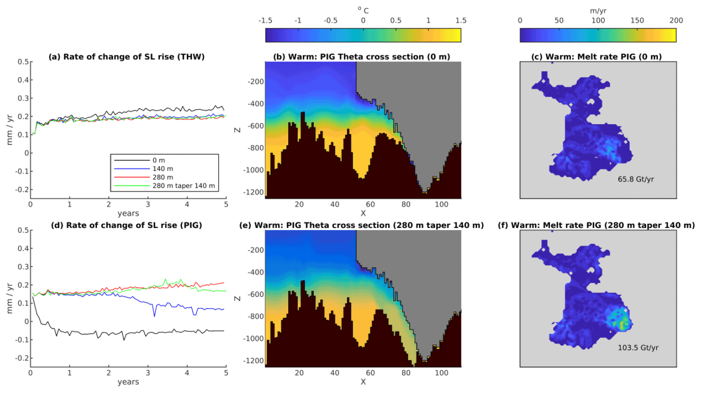
Figure C1(a) SLR rate of change for the Thwaites area for zero deepening, 140 m deepening, 280 m deepening and 280 m deepening tapering to 140 m over 6 km. (b) Cross-section through PIG Ice Shelf (taken along the green line shown in Fig. 2a) showing initial potential temperature in the warm case in the zero-deepening setup. (c) Initial melt rate over PIG Ice Shelf in the warm forcing case for the zero-deepening setup. (d) Same as (a), but for the PIG area. (e) Same as (b), but for the 280 m tapering 140 m deepening setup. (f) Same as (c), but for the 280 m tapering 140 m deepening setup.
Therefore, an initial deepening step was applied in order to prevent re-grounding and minimise any changes in SLR rate at the start of the simulation (Fig. C1d). However, enforcing a uniform minimum water column thickness everywhere would create a sudden step-change in the bathymetry at the initial grounding-line location. Therefore, a taper is applied to the water column thickness used in the deepening procedure, increasing the minimum thickness from a low value at the grounding line to its standard value over 6 km distance. After applying this initial deepening procedure, PIG does not re-ground at the start of the simulation. We note that the SLR rate from the Thwaites region (Fig. C1a) is only minimally affected by the deepening procedure. While the deepening of the PIG water column is somewhat subjective, the deeper water column better reflects the sparsely available observations of the cavity near the grounding line (Dutrieux et al., 2014). Overall, the necessity of deepening emphasises the importance of obtaining more detailed observations of the geometry of ice shelf cavities, beneath PIG in particular.
A strong correlation is found when comparing the sea level contribution against the integrated melt for both forcing cases in the areas of Thwaites and PIG (Fig. D1). However, no variation to the oceanic boundary forcing is applied during the simulations, and hence only geometric-induced changes in the ice shelf melt rates can occur. These strong correlations are due to the melt rate and rate of change of SLR being approximately constant from PIG's area and having an approximately linear trend from Thwaites's area. The regression between the SLR contribution and the integrated melt for both the Thwaites and PIG areas are different for the two oceanographic forcings applied, which suggests that the ratio of mass loss between ice shelf melting and calving is different between the cases, with the warm case having a higher relative ice shelf melting.
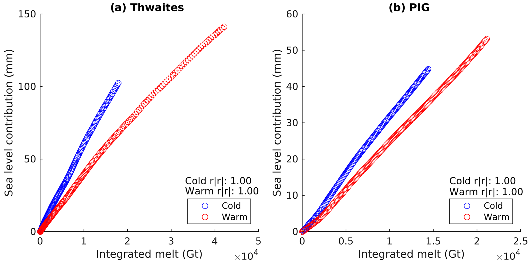
Figure D1(a) Yearly points of sea level contribution plotted against integrated melt from the Thwaites area for the warm (red) and cold (blue) forcing cases. Panel (b) as in (a), but for the PIG area. In both, correlation coefficients are shown for the warm and cold cases.
The version of MITgcm used in this study is available at https://github.com/David-Bett4/MITgcm/tree/Coupling_wHoriz_lat_Pchild_new_divout (commit 26ffb9f, last access: 30 May 2024) and https://doi.org/10.5281/zenodo.11394744 (Campin et al., 2024). The version of WAVI used in this study is available at https://github.com/David-Bett4/WAVI.jl/tree/MITgcm_coupling (commit 7c292f1, last access: 30 May 2024) and https://doi.org/10.5281/zenodo.11389948 (Bradley et al., 2024). Coupling scripts and input text files are available at https://github.com/David-Bett4/MITgcm_WAVI_coupling and https://doi.org/10.5281/zenodo.11384525 (Bett et al., 2024a). The model output underlying the figures and calculations in this paper is available through the UK Polar Data Centre (https://doi.org/10.5285/baa5097e-5139-4d8b-8986-3cc84c3319b7, Bett et al., 2024b).
DTB implemented coupling, set up ocean initial state, ran coupled simulations, performed analysis and led the manuscript writing. ATB and CRW set up initial WAVI ice model states and performed WAVI ice model relaxation simulations. RJA, PRH, CRW and DNG designed and supervised the project. All of the co-authors contributed to coupling design, experiment design and editing the manuscript.
The contact author has declared that none of the authors has any competing interests.
Publisher's note: Copernicus Publications remains neutral with regard to jurisdictional claims made in the text, published maps, institutional affiliations, or any other geographical representation in this paper. While Copernicus Publications makes every effort to include appropriate place names, the final responsibility lies with the authors.
This work used the ARCHER2 UK National Supercomputing Service (https://www.archer2.ac.uk, last access: 1 March 2024). The authors thank the two anonymous reviewers for their careful reading of the manuscript and their helpful comments.
David T. Bett, Alexander T. Bradley, C. Rosie Williams, Paul R. Holland and Robert J. Arthern were supported by the NERC grant NE/S010475/1. C. Rosie Williams was partly funded by the MELT project, a component of the International Thwaites Glacier Collaboration (ITGC), with support from the National Science Foundation (NSF: grant no. 1739003) and Natural Environment Research Council (NERC: grant no. NE/S006656/1). Daniel N. Goldberg acknowledges support from ITGC project PROPHET, ITGC contribution no. ITGC-108. This publication was supported by PROTECT. This project has received funding from the European Union's Horizon 2020 research and innovation programme (grant no. 869304), PROTECT contribution number 93.
This paper was edited by Nicolas Jourdain and reviewed by two anonymous referees.
Alevropoulos-Borrill, A. V., Nias, I. J., Payne, A. J., Golledge, N. R., and Bingham, R. J.: Ocean-forced evolution of the Amundsen Sea catchment, West Antarctica, by 2100, The Cryosphere, 14, 1245–1258, https://doi.org/10.5194/tc-14-1245-2020, 2020.
Arthern, R. J. and Williams, C. R.: The sensitivity of West Antarctica to the submarine melting feedback, Geophys. Res. Lett., 44, 2352–2359, https://doi.org/10.1002/2017GL072514, 2017.
Arthern, R. J., Winebrenner, D. P., and Vaughan, D. G.: Antarctic snow accumulation mapped using polarization of 4.3-cm wavelength microwave emission, J. Geophys. Res.-Atmos., 111, D06107, https://doi.org/10.1029/2004JD005667, 2006.
Arthern, R. J., Hindmarsh, R. C. A., and Williams, C. R.: Flow speed within the Antarctic ice sheet and its controls inferred from satellite observations, J. Geophys. Res.-Earth Surf., 120, 1171–1188, https://doi.org/10.1002/2014JF003239, 2015.
Asay-Davis, X. S., Jourdain, N. C., and Nakayama, Y.: Developments in Simulating and Parameterizing Interactions Between the Southern Ocean and the Antarctic Ice Sheet, Current Climate Change Reports, 3, 316–329, https://doi.org/10.1007/s40641-017-0071-0, 2017.
Bett, D. T., Holland, P. R., Naveira Garabato, A. C., Jenkins, A., Dutrieux, P., Kimura, S., and Fleming, A.: The Impact of the Amundsen Sea Freshwater Balance on Ocean Melting of the West Antarctic Ice Sheet, J. Geophys. Res.-Oceans, 125, e2020JC016305, https://doi.org/10.1029/2020JC016305, 2020.
Bett, D. T., Bradley, A. T., Williams, R., Holland, P. R., Arthern, R. J., and Goldberg, D. N.: MITgcm and WAVI coupling scripts, Zenodo [code], https://doi.org/10.5281/zenodo.11384525, 2024a.
Bett, D. T., Bradley, A. T., Williams, R., Holland, P. R., Arthern, R. J., and Goldberg, D. N.: Amundsen Sea sector MITgcm/WAVI coupled model output forced with idealised ocean boundary conditions over 180 years (Version 1.0), NERC EDS UK Polar Data Centre [data set], https://doi.org/10.5285/baa5097e-5139-4d8b-8986-3cc84c3319b7, 2024b.
Bradley, A. T., Bett, D. T., Dutrieux, P., De Rydt, J., and Holland, P. R.: The Influence of Pine Island Ice Shelf Calving on Basal Melting, J. Geophys. Res.-Oceans, 127, e2022JC018621, https://doi.org/10.1029/2022JC018621, 2022.
Bradley, A., Arthern, R., Williams, R., Bett, D., and Thodoroff, P.: David-Bett4/WAVI.jl: Release of WAVI with MITgcm coupling (v0.0.2-coupling), Zenodo [code], https://doi.org/10.5281/zenodo.11389948, 2024.
Brondex, J., Gillet-Chaulet, F., and Gagliardini, O.: Sensitivity of centennial mass loss projections of the Amundsen basin to the friction law, The Cryosphere, 13, 177–195, https://doi.org/10.5194/tc-13-177-2019, 2019.
Burgard, C., Jourdain, N. C., Reese, R., Jenkins, A., and Mathiot, P.: An assessment of basal melt parameterisations for Antarctic ice shelves, The Cryosphere, 16, 4931–4975, https://doi.org/10.5194/tc-16-4931-2022, 2022.
Campin, J.-M., Heimbach, Patrick, Losch, M., Forget, G., edhill, Adcroft, A., amolod, Menemenlis, D., dfer22, Hill, C., Jahn, O., Scott, J., stephdut, Mazloff, M., Fox-Kemper, B., antnguyen13, Doddridge, E., Fenty, I., Bates, M., Eichmann, A., Smith, T., mitllheisey, Martin, T., Lauderdale, J., Abernathey, R., samarkhatiwala, hongandyan, Deremble, B., dngoldberg, and Wang, O.: David-Bett4/MITgcm: Release of MITgcm with WAVI coupling (v1.0.0), Zenodo [code], https://doi.org/10.5281/zenodo.11394744, 2024.
Cornford, S. L., Gladstone, R. M., and Payne, A. J.: Resolution requirements for grounding-line modelling: sensitivity to basal drag and ice-shelf buttressing, Ann. Glaciol., 53, 97–105, https://doi.org/10.3189/2012AoG60A148, 2012.
Cornford, S. L., Seroussi, H., Asay-Davis, X. S., Gudmundsson, G. H., Arthern, R., Borstad, C., Christmann, J., Dias dos Santos, T., Feldmann, J., Goldberg, D., Hoffman, M. J., Humbert, A., Kleiner, T., Leguy, G., Lipscomb, W. H., Merino, N., Durand, G., Morlighem, M., Pollard, D., Rückamp, M., Williams, C. R., and Yu, H.: Results of the third Marine Ice Sheet Model Intercomparison Project (MISMIP+), The Cryosphere, 14, 2283–2301, https://doi.org/10.5194/tc-14-2283-2020, 2020.
De Rydt, J. and Gudmundsson, G. H.: Coupled ice shelf-ocean modeling and complex grounding line retreat from a seabed ridge, J. Geophys. Res.-Earth Surf., 121, 865–880, https://doi.org/10.1002/2015JF003791, 2016.
De Rydt, J., Holland, P. R., Dutrieux, P., and Jenkins, A.: Geometric and oceanographic controls on melting beneath Pine Island Glacier, J. Geophys. Res.-Oceans, 119, 2420–2438, https://doi.org/10.1002/2013JC009513, 2014.
Donat-Magnin, M., Jourdain, N. C., Spence, P., Le Sommer, J., Gallée, H., and Durand, G.: Ice-Shelf Melt Response to Changing Winds and Glacier Dynamics in the Amundsen Sea Sector, Antarctica, J. Geophys. Res.-Oceans, 122, 10206–10224, https://doi.org/10.1002/2017JC013059, 2017.
Dutrieux, P., De Rydt, J., Jenkins, A., Holland, P. R., Ha, H. K., Lee, S. H., Steig, E. J., Ding, Q., Abrahamsen, E. P., and Schröder, M.: Strong Sensitivity of Pine Island Ice-Shelf Melting to Climatic Variability, Science, 343, 174–178, https://doi.org/10.1126/science.1244341, 2014.
Edwards, T. L., Nowicki, S., Marzeion, B., Hock, R., Goelzer, H., Seroussi, H., Jourdain, N. C., Slater, D. A., Turner, F. E., Smith, C. J., McKenna, C. M., Simon, E., Abe-Ouchi, A., Gregory, J. M., Larour, E., Lipscomb, W. H., Payne, A. J., Shepherd, A., Agosta, C., Alexander, P., Albrecht, T., Anderson, B., Asay-Davis, X., Aschwanden, A., Barthel, A., Bliss, A., Calov, R., Chambers, C., Champollion, N., Choi, Y., Cullather, R., Cuzzone, J., Dumas, C., Felikson, D., Fettweis, X., Fujita, K., Galton-Fenzi, B. K., Gladstone, R., Golledge, N. R., Greve, R., Hattermann, T., Hoffman, M. J., Humbert, A., Huss, M., Huybrechts, P., Immerzeel, W., Kleiner, T., Kraaijenbrink, P., Le clec'h, S., Lee, V., Leguy, G. R., Little, C. M., Lowry, D. P., Malles, J.-H., Martin, D. F., Maussion, F., Morlighem, M., O'Neill, J. F., Nias, I., Pattyn, F., Pelle, T., Price, S. F., Quiquet, A., Radiæ, V., Reese, R., Rounce, D. R., Rückamp, M., Sakai, A., Shafer, C., Schlegel, N.-J., Shannon, S., Smith, R. S., Straneo, F., Sun, S., Tarasov, L., Trusel, L. D., Van Breedam, J., van de Wal, R., van den Broeke, M., Winkelmann, R., Zekollari, H., Zhao, C., Zhang, T., and Zwinger, T.: Projected land ice contributions to twenty-first-century sea level rise, Nature, 593, 74–82, https://doi.org/10.1038/s41586-021-03302-y, 2021.
Favier, L., Durand, G., Cornford, S. L., Gudmundsson, G. H., Gagliardini, O., Gillet-Chaulet, F., Zwinger, T., Payne, A. J., and Le Brocq, A. M.: Retreat of Pine Island Glacier controlled by marine ice-sheet instability, Nat. Clim. Change, 4, 117–121, https://doi.org/10.1038/nclimate2094, 2014.
Feldmann, J. and Levermann, A.: Collapse of the West Antarctic Ice Sheet after local destabilization of the Amundsen Basin, P. Natl. Acad. Sci. USA, 112, 14191–14196, https://doi.org/10.1073/pnas.1512482112, 2015.
Goldberg, D. N.: A variationally derived, depth-integrated approximation to a higher-order glaciological flow model, J. Glaciol., 57, 157–170, https://doi.org/10.3189/002214311795306763, 2011.
Goldberg, D. N. and Heimbach, P.: Parameter and state estimation with a time-dependent adjoint marine ice sheet model, The Cryosphere, 7, 1659–1678, https://doi.org/10.5194/tc-7-1659-2013, 2013.
Goldberg, D. N. and Holland, P. R.: The Relative Impacts of Initialization and Climate Forcing in Coupled Ice Sheet-Ocean Modeling: Application to Pope, Smith, and Kohler Glaciers, J. Geophys. Res.-Earth Surf., 127, e2021JF006570, https://doi.org/10.1029/2021JF006570, 2022.
Goldberg, D. N., Snow, K., Holland, P., Jordan, J. R., Campin, J. M., Heimbach, P., Arthern, R., and Jenkins, A.: Representing grounding line migration in synchronous coupling between a marine ice sheet model and a z-coordinate ocean model, Ocean Model., 125, 45–60, https://doi.org/10.1016/j.ocemod.2018.03.005, 2018.
Graham, A. G. C., Wåhlin, A., Hogan, K. A., Nitsche, F. O., Heywood, K. J., Totten, R. L., Smith, J. A., Hillenbrand, C.-D., Simkins, L. M., Anderson, J. B., Wellner, J. S., and Larter, R. D.: Rapid retreat of Thwaites Glacier in the pre-satellite era, Nat. Geosci., 15, 706–713, https://doi.org/10.1038/s41561-022-01019-9, 2022.
Gudmundsson, G. H., Barnes, J. M., Goldberg, D. N., and Morlighem, M.: Limited Impact of Thwaites Ice Shelf on Future Ice Loss From Antarctica, Geophys. Res. Lett., 50, e2023GL102880, https://doi.org/10.1029/2023GL102880, 2023.
Hill, E. A., Urruty, B., Reese, R., Garbe, J., Gagliardini, O., Durand, G., Gillet-Chaulet, F., Gudmundsson, G. H., Winkelmann, R., Chekki, M., Chandler, D., and Langebroek, P. M.: The stability of present-day Antarctic grounding lines – Part 1: No indication of marine ice sheet instability in the current geometry, The Cryosphere, 17, 3739–3759, https://doi.org/10.5194/tc-17-3739-2023, 2023.
Holland, D. M. and Jenkins, A.: Modeling Thermodynamic Ice–Ocean Interactions at the Base of an Ice Shelf, J. Phys. Oceanogr., 29, 1787–1800, https://doi.org/10.1175/1520-0485(1999)029<1787:MTIOIA>2.0.CO;2, 1999.
Holland, P. R. and Feltham, D. L.: The Effects of Rotation and Ice Shelf Topography on Frazil-Laden Ice Shelf Water Plumes, J. Phys. Oceanogr., 36, 2312–2327, https://doi.org/10.1175/JPO2970.1, 2006.
Holland, P. R., Bracegirdle, T. J., Dutrieux, P., Jenkins, A., and Steig, E. J.: West Antarctic ice loss influenced by internal climate variability and anthropogenic forcing, Nat. Geosci., 12, 718–724, https://doi.org/10.1038/s41561-019-0420-9, 2019.
Holland, P. R., O'Connor, G. K., Bracegirdle, T. J., Dutrieux, P., Naughten, K. A., Steig, E. J., Schneider, D. P., Jenkins, A., and Smith, J. A.: Anthropogenic and internal drivers of wind changes over the Amundsen Sea, West Antarctica, during the 20th and 21st centuries, The Cryosphere, 16, 5085–5105, https://doi.org/10.5194/tc-16-5085-2022, 2022.
Holland, P. R., Bevan, S. L., and Luckman, A. J.: Strong Ocean Melting Feedback During the Recent Retreat of Thwaites Glacier, Geophys. Res. Lett., 50, e2023GL103088, https://doi.org/10.1029/2023GL103088, 2023.
Jacobs, S. S., Hellmer, H. H., and Jenkins, A.: Antarctic ice sheet melting in the Southeast Pacific, Geophys. Res. Lett., 23, 957–960, https://doi.org/10.1029/96gl00723, 1996.
Jenkins, A., Nicholls, K. W., and Corr, H. F. J.: Observation and Parameterization of Ablation at the Base of Ronne Ice Shelf, Antarctica, J. Phys. Oceanogr., 40, 2298–2312, https://doi.org/10.1175/2010JPO4317.1, 2010.
Jenkins, A., Shoosmith, D., Dutrieux, P., Jacobs, S., Kim, T. W., Lee, S. H., Ha, H. K., and Stammerjohn, S.: West Antarctic Ice Sheet retreat in the Amundsen Sea driven by decadal oceanic variability, Nat. Geosci., 11, 733–738, https://doi.org/10.1038/s41561-018-0207-4, 2018.
Jordan, J. R., Holland, P. R., Goldberg, D., Snow, K., Arthern, R., Campin, J.-M., Heimbach, P., and Jenkins, A.: Ocean-Forced Ice-Shelf Thinning in a Synchronously Coupled Ice-Ocean Model, J. Geophys. Res.-Oceans, 123, 864–882, https://doi.org/10.1002/2017JC013251, 2018.
Joughin, I., Smith, B. E., and Medley, B.: Marine Ice Sheet Collapse Potentially Under Way for the Thwaites Glacier Basin, West Antarctica, Science, 344, 735–738, https://doi.org/10.1126/science.1249055, 2014.
Joughin, I., Shapero, D., Smith, B., Dutrieux, P., and Barham, M.: Ice-shelf retreat drives recent Pine Island Glacier speedup, Sci. Adv., 7, eabg3080, https://doi.org/10.1126/sciadv.abg3080, 2021.
Jourdain, N. C., Mathiot, P., Burgard, C., Caillet, J., and Kittel, C.: Ice Shelf Basal Melt Rates in the Amundsen Sea at the End of the 21st Century, Geophys. Res. Lett., 49, e2022GL100629, https://doi.org/10.1029/2022GL100629, 2022.
Jourdain, N. C., Mathiot, P., Merino, N., Durand, G., Le Sommer, J., Spence, P., Dutrieux, P., and Madec, G.: Ocean circulation and sea-ice thinning induced by melting ice shelves in the Amundsen Sea, J. Geophys. Res.-Oceans, 122, 2550–2573, https://doi.org/10.1002/2016JC012509, 2017.
Kimura, S., Jenkins, A., Regan, H., Holland, P. R., Assmann, K. M., Whitt, D. B., Van Wessem, M., van de Berg, W. J., Reijmer, C. H., and Dutrieux, P.: Oceanographic Controls on the Variability of Ice-Shelf Basal Melting and Circulation of Glacial Meltwater in the Amundsen Sea Embayment, Antarctica, J. Geophys. Res.-Oceans, 122, 10131–10155, https://doi.org/10.1002/2017JC012926, 2017.
Lhermitte, S., Sun, S., Shuman, C., Wouters, B., Pattyn, F., Wuite, J., Berthier, E., and Nagler, T.: Damage accelerates ice shelf instability and mass loss in Amundsen Sea Embayment, P. Natl. Acad. Sci. USA, 117, 24735–24741, https://doi.org/10.1073/pnas.1912890117, 2020.
Marshall, J., Hill, C., Perelman, L., and Adcroft, A.: Hydrostatic, quasi-hydrostatic, and nonhydrostatic ocean modeling, J. Geophys. Res.-Oceans, 102, 5733–5752, https://doi.org/10.1029/96JC02776, 1997.
Morlighem, M.: MEaSUREs BedMachine Antarctica, Version 3, Boulder, Colorado USA. NASA National Snow and Ice Data Center Distributed Active Archive Center [data set], https://doi.org/10.5067/FPSU0V1MWUB6, 2022.
Morlighem, M., Rignot, E., Binder, T., Blankenship, D., Drews, R., Eagles, G., Eisen, O., Ferraccioli, F., Forsberg, R., Fretwell, P., Goel, V., Greenbaum, J. S., Gudmundsson, H., Guo, J., Helm, V., Hofstede, C., Howat, I., Humbert, A., Jokat, W., Karlsson, N. B., Lee, W. S., Matsuoka, K., Millan, R., Mouginot, J., Paden, J., Pattyn, F., Roberts, J., Rosier, S., Ruppel, A., Seroussi, H., Smith, E. C., Steinhage, D., Sun, B., Broeke, M. R. v. d., Ommen, T. D. v., Wessem, M. v., and Young, D. A.: Deep glacial troughs and stabilizing ridges unveiled beneath the margins of the Antarctic ice sheet, Nat. Geosci., 13, 132–137, https://doi.org/10.1038/s41561-019-0510-8, 2020.
Mouginot, J., Rignot, E., and Scheuchl, B.: Sustained increase in ice discharge from the Amundsen Sea Embayment, West Antarctica, from 1973 to 2013, Geophys. Res. Lett., 41, 1576–1584, https://doi.org/10.1002/2013GL059069, 2014.
Mouginot, J., Rignot, E., Scheuchl, B., and Millan, R.: Comprehensive Annual Ice Sheet Velocity Mapping Using Landsat-8, Sentinel-1, and RADARSAT-2 Data, Remote Sens.-Basel, 9, 364, https://doi.org/10.3390/rs9040364, 2017a.
Mouginot, J., Scheuchl, B., and Rignot, E.: MEaSUREs Annual Antarctic Ice Velocity Maps, Version 1, Boulder, Colorado USA. NASA National Snow and Ice Data Center Distributed Active Archive Center [data set], https://doi.org/10.5067/9T4EPQXTJYW9, 2017b.
Nakayama, Y., Cai, C., and Seroussi, H.: Impact of Subglacial Freshwater Discharge on Pine Island Ice Shelf, Geophys. Res. Lett., 48, e2021GL093923, https://doi.org/10.1029/2021GL093923, 2021.
Naughten, K. A., De Rydt, J., Rosier, S. H. R., Jenkins, A., Holland, P. R., and Ridley, J. K.: Two-timescale response of a large Antarctic ice shelf to climate change, Nat. Commun., 12, 1991, https://doi.org/10.1038/s41467-021-22259-0, 2021.
Naughten, K. A., Holland, P. R., Dutrieux, P., Kimura, S., Bett, D. T., and Jenkins, A.: Simulated Twentieth-Century Ocean Warming in the Amundsen Sea, West Antarctica, Geophys. Res. Lett., 49, e2021GL094566, https://doi.org/10.1029/2021GL094566, 2022.
Naughten, K. A., Holland, P. R., and De Rydt, J.: Unavoidable future increase in West Antarctic ice-shelf melting over the twenty-first century, Nat. Clim. Change, 13, 1222–1228, https://doi.org/10.1038/s41558-023-01818-x, 2023.
Nias, I. J., Cornford, S. L., Edwards, T. L., Gourmelen, N., and Payne, A. J.: Assessing Uncertainty in the Dynamical Ice Response to Ocean Warming in the Amundsen Sea Embayment, West Antarctica, Geophys. Res. Lett., 46, 11253–11260, https://doi.org/10.1029/2019GL084941, 2019.
Otosaka, I. N., Shepherd, A., Ivins, E. R., Schlegel, N.-J., Amory, C., van den Broeke, M. R., Horwath, M., Joughin, I., King, M. D., Krinner, G., Nowicki, S., Payne, A. J., Rignot, E., Scambos, T., Simon, K. M., Smith, B. E., Sørensen, L. S., Velicogna, I., Whitehouse, P. L., A, G., Agosta, C., Ahlstrøm, A. P., Blazquez, A., Colgan, W., Engdahl, M. E., Fettweis, X., Forsberg, R., Gallée, H., Gardner, A., Gilbert, L., Gourmelen, N., Groh, A., Gunter, B. C., Harig, C., Helm, V., Khan, S. A., Kittel, C., Konrad, H., Langen, P. L., Lecavalier, B. S., Liang, C.-C., Loomis, B. D., McMillan, M., Melini, D., Mernild, S. H., Mottram, R., Mouginot, J., Nilsson, J., Noël, B., Pattle, M. E., Peltier, W. R., Pie, N., Roca, M., Sasgen, I., Save, H. V., Seo, K.-W., Scheuchl, B., Schrama, E. J. O., Schröder, L., Simonsen, S. B., Slater, T., Spada, G., Sutterley, T. C., Vishwakarma, B. D., van Wessem, J. M., Wiese, D., van der Wal, W., and Wouters, B.: Mass balance of the Greenland and Antarctic ice sheets from 1992 to 2020, Earth Syst. Sci. Data, 15, 1597–1616, https://doi.org/10.5194/essd-15-1597-2023, 2023.
Pattyn, F.: Antarctic subglacial conditions inferred from a hybrid ice sheet/ice stream model, Earth Planet. Sc. Lett., 295, 451–461, https://doi.org/10.1016/j.epsl.2010.04.025, 2010.
Pattyn, F., Huyghe, A., De Brabander, S., and De Smedt, B.: Role of transition zones in marine ice sheet dynamics, J. Geophys. Res.-Earth Surf., 111, https://doi.org/10.1029/2005JF000394, 2006.
Reese, R., Levermann, A., Albrecht, T., Seroussi, H., and Winkelmann, R.: The role of history and strength of the oceanic forcing in sea level projections from Antarctica with the Parallel Ice Sheet Model, The Cryosphere, 14, 3097–3110, https://doi.org/10.5194/tc-14-3097-2020, 2020.
Reese, R., Garbe, J., Hill, E. A., Urruty, B., Naughten, K. A., Gagliardini, O., Durand, G., Gillet-Chaulet, F., Gudmundsson, G. H., Chandler, D., Langebroek, P. M., and Winkelmann, R.: The stability of present-day Antarctic grounding lines – Part 2: Onset of irreversible retreat of Amundsen Sea glaciers under current climate on centennial timescales cannot be excluded, The Cryosphere, 17, 3761–3783, https://doi.org/10.5194/tc-17-3761-2023, 2023.
Schoof, C.: Ice sheet grounding line dynamics: Steady states, stability, and hysteresis, J. Geophys. Res.-Earth Surf., 112, F03S28, https://doi.org/10.1029/2006JF000664, 2007.
Seroussi, H. and Morlighem, M.: Representation of basal melting at the grounding line in ice flow models, The Cryosphere, 12, 3085–3096, https://doi.org/10.5194/tc-12-3085-2018, 2018.
Seroussi, H., Morlighem, M., Larour, E., Rignot, E., and Khazendar, A.: Hydrostatic grounding line parameterization in ice sheet models, The Cryosphere, 8, 2075–2087, https://doi.org/10.5194/tc-8-2075-2014, 2014.
Seroussi, H., Nakayama, Y., Larour, E., Menemenlis, D., Morlighem, M., Rignot, E., and Khazendar, A.: Continued retreat of Thwaites Glacier, West Antarctica, controlled by bed topography and ocean circulation, Geophys. Res. Lett., 44, 6191–6199, https://doi.org/10.1002/2017GL072910, 2017.
Shepherd, A., Gilbert, L., Muir, A. S., Konrad, H., McMillan, M., Slater, T., Briggs, K. H., Sundal, A. V., Hogg, A. E., and Engdahl, M. E.: Trends in Antarctic Ice Sheet Elevation and Mass, Geophys. Res. Lett., 46, 8174–8183, https://doi.org/10.1029/2019GL082182, 2019.
Smith, B., Fricker, H. A., Gardner, A. S., Medley, B., Nilsson, J., Paolo, F. S., Holschuh, N., Adusumilli, S., Brunt, K., Csatho, B., Harbeck, K., Markus, T., Neumann, T., Siegfried, M. R., and Zwally, H. J.: Pervasive ice sheet mass loss reflects competing ocean and atmosphere processes, Science, 368, 1239–1242, https://doi.org/10.1126/science.aaz5845, 2020.
St-Laurent, P., Klinck, J. M., and Dinniman, M. S.: Impact of local winter cooling on the melt of Pine Island Glacier, Antarctica, J. Geophys. Res.-Oceans, 120, 6718–6732, https://doi.org/10.1002/2015JC010709, 2015.
Thomas, R. H.: The Dynamics of Marine Ice Sheets, J. Glaciol., 24, 167–177, https://doi.org/10.3189/S0022143000014726, 1979.
Walker, D. P., Brandon, M. A., Jenkins, A., Allen, J. T., Dowdeswell, J. A., and Evans, J.: Oceanic heat transport onto the Amundsen Sea shelf through a submarine glacial trough, Geophys. Res. Lett., 34, L02602, https://doi.org/10.1029/2006gl028154, 2007.
Webber, B. G. M., Heywood, K. J., Stevens, D. P., Dutrieux, P., Abrahamsen, E. P., Jenkins, A., Jacobs, S. S., Ha, H. K., Lee, S. H., and Kim, T. W.: Mechanisms driving variability in the ocean forcing of Pine Island Glacier, Nat. Commun., 8, 14507, https://doi.org/10.1038/ncomms14507, 2017.
Weertman, J.: The Theory of Glacier Sliding, J. Glaciol., 5, 287–303, https://doi.org/10.3189/S0022143000029038, 1964.
Weertman, J.: Stability of the Junction of an Ice Sheet and an Ice Shelf, J. Glaciol., 13, 3–11, https://doi.org/10.3189/S0022143000023327, 1974.
Wild, C. T., Alley, K. E., Muto, A., Truffer, M., Scambos, T. A., and Pettit, E. C.: Weakening of the pinning point buttressing Thwaites Glacier, West Antarctica, The Cryosphere, 16, 397–417, https://doi.org/10.5194/tc-16-397-2022, 2022.
Williams, C., Thodoroff, P., Arthern, R., Byrne, J., Hosking, J. S., Kaiser, M., Lawrence, N., and Kazlauskaite, I.: Calculating exposure to extreme sea level risk will require high resolution ice sheet models, Research Square, Nature Portfolio, in review, https://doi.org/10.21203/rs.3.rs-3405435/v1, 2024.
Yu, H., Rignot, E., Seroussi, H., and Morlighem, M.: Retreat of Thwaites Glacier, West Antarctica, over the next 100 years using various ice flow models, ice shelf melt scenarios and basal friction laws, The Cryosphere, 12, 3861–3876, https://doi.org/10.5194/tc-12-3861-2018, 2018.
Zwally, H. J., Giovinetto, M. B., Matthew, A. B., and Jack, L. S.: Antarctic and Greenland Drainage Systems, GSFC Cryospheric Sciences Laboratory, https://earth.gsfc.nasa.gov/cryo/data/polar-altimetry/antarctic-and-greenland-drainage-systems (last access: 5 February 2024), 2012.
- Abstract
- Introduction
- Methods
- Results
- Discussion
- Conclusions
- Appendix A: Ice model relaxation comparison
- Appendix B: Ice shelf melt rate tuning
- Appendix C: Initial bathymetry deepening
- Appendix D: SLR compared against integrated melt
- Code and data availability
- Author contributions
- Competing interests
- Disclaimer
- Acknowledgements
- Financial support
- Review statement
- References