Modeling snowpack dynamics and surface energy budget in boreal and subarctic peatlands and forests

The snowpack has a major influence on the land surface energy budget. Accurate simulation of the snowpack energy and radiation budget is challenging due to, e.g., effects of vegetation and topography, as well as limitations in the theoretical understanding of turbulent transfer in the stable boundary layer. Studies that evaluate snow, hydrology and land surface models against detailed observations of all surface energy balance components at high latitudes are scarce. In this study, we compared different configurations of the SURFEX land surface model against surface energy flux, snow depth and soil temperature observations from four eddy-covariance stations in Finland. The sites cover two different climate and snow conditions, representing the southern and northern subarctic zones, as well as the contrasting forest and peatland ecosystems typical for the boreal landscape. We tested different turbulent flux parameterizations implemented in the Crocus snowpack model. In addition, we examined common alternative approaches to conceptualize soil and vegetation, and we assessed their performance in simulating surface energy fluxes, snow conditions and soil thermal regime. Our results show that a stability correction function that increases the turbulent exchange under stable atmospheric conditions is imperative to simulate sensible heat fluxes over the peatland snowpacks and that realistic peat soil texture (soil organic content) parameterization greatly improves the soil temperature simulations. For accurate simulations of surface energy fluxes, snow and soil conditions in forests, an explicit vegetation representation is necessary. Moreover, we demonstrate the high sensitivity of surface fluxes to a poorly documented parameter involved in snow cover fraction computation. Although we focused on models within the SURFEX platform, the results have broader implications for choosing suitable turbulent flux parameterization and model structures depending on the potential use cases for high-latitude land surface modeling.

1 Introduction

The boreal zone, characterized by a mosaic of seasonally snow-covered peatlands, forests and lakes, is the largest land biome in the world. Snow conditions in the boreal zone are rapidly changing due to climate warming, which is found to be the strongest during the cold seasons in the Arctic (Serreze et al., 2009; Screen and Simmonds, 2010; Boisvert and Stroeve, 2015; Rantanen et al., 2022). Evidently snow has an important role for water resources and human activities in the cold regions, but it is also known that the snowpack characteristics affect animal movement (Tyler, 2010; Pedersen et al., 2021) and plant distribution (Rasmus et al., 2011; Kreyling et al., 2012; Rissanen et al., 2021). Recent studies show that especially cold-dwelling species have been shifting towards higher latitudes and altitudes in search for more suitable habitats (Tayleur et al., 2016; Couet et al., 2022). Therefore, the rapid warming of the Arctic and its consequences on the quantity and properties of snow may define the destiny of many species and human activities in the boreal region. To predict future snow conditions, environmental change, and the consequences for water resources, ecosystems and people, predictive and process-based models possess great potential (Clark et al., 2015; Boone et al., 2017). Land surface models (LSMs) have been used for decades in numerical weather prediction and in global circulation models (Douville et al., 1995; Niu et al., 2011; Lawrence et al., 2019) and have more recently become common tools for interdisciplinary impact studies (Blyth et al., 2021).

Snowpack has a major impact on the wintertime energy budget due to its influence on the land surface albedo (hereafter albedo) and the surface heat fluxes (Cohen and Rind, 1991; Eugster et al., 2000). The heat diffusion within the snowpack is determined by the surface heat fluxes, internal properties of the snowpack and soil thermal regime. Correctly representing the snowpack is thus essential for simulating energy and mass exchange between the snow surface and the atmosphere, as well as below the snowpack (e.g., surface temperatures and soil freezing–thawing dynamics, Koivusalo and Heikinheimo, 1999; Slater et al., 2001). The snowpack energy budget is partitioned into downward and upward shortwave and longwave radiation, turbulent fluxes of sensible and latent heat, snowpack–ground heat flux, and phase changes in the snow. The snowpack energy balance and energy partitioning among the flux components vary strongly across diurnal and seasonal timescales, as well as between different ecosystems (Clark et al., 2011; Stiegler et al., 2016; Stigter et al., 2021). It is essential that LSMs are able to correctly reproduce this variability.

On the vast boreal and arctic peatlands with shallow vegetation, the snow cover can exclusively determine the wintertime albedo (Aurela et al., 2015). With minimal solar radiation during winter months on these open snow fields, turbulent fluxes make an important component in the energy budget of the snowpack, as they compensate for the radiative cooling processes and further contribute to snowmelt (Lackner et al., 2022; Conway et al., 2018). Simulation of turbulent fluxes under stable atmospheric conditions is known as one of the major sources of uncertainty in snow models (Lafaysse et al., 2017; Menard et al., 2021). In LSMs the turbulent fluxes are commonly computed with bulk aerodynamic approaches, where sensible and latent heat fluxes are proportional to the turbulent exchange coefficient according to the Monin–Obukhov similarity theory. These approaches typically use atmospheric stability correction functions based either on the bulk Richardson number (Martin and Lejeune, 1998; Lafaysse et al., 2017; Clark et al., 2015) or the Obukhov length scale (Jordan et al., 1999). It is established that the Monin–Obukhov similarity theory does not well represent low-wind and stable atmospheric conditions above aerodynamically smooth surfaces such as snow (Conway et al., 2018). In such conditions, the simulated surface temperatures have been found to be unrealistically low, as the turbulent boundary layer tends to decouple from the snow surface (Derbyshire, 1999; Andreas et al., 2010). To circumvent this effect, stability correction functions have been modified to permit turbulent fluxes above critical stability thresholds (Lafaysse et al., 2017) by manipulating the wind speed (Martin and Lejeune, 1998; Andreas et al., 2010) or including a windless turbulent exchange coefficient (Jordan et al., 1999). Evaluations of these modifications often rely on validation with observed surface temperatures and snow depths (e.g., for the detailed snowpack model Crocus; Martin and Lejeune, 1998; Lafaysse et al., 2017), while comparisons against turbulent energy flux data remain scarce (Lapo et al., 2019; Conway et al., 2018).

The energy budgets of forest canopies and below-canopy snowpack are different to those on open peatlands, as turbulent exchange is attenuated by the canopy, and the snowpack energy budget and snowmelt are mostly driven by the radiation balance (Rutter et al., 2009; Essery et al., 2009; Varhola et al., 2010). However, due to heterogeneous canopy structures and canopy processes (radiation transmittance, snow interception and unloading) together with low solar angles, the albedo dynamics of seasonally snow-covered boreal forests is complex (Malle et al., 2021). The absorption of the shortwave radiation can be highly heterogeneous, having direct implications on canopy temperatures (Webster et al., 2017) and on the resulting longwave radiative fluxes between canopy, snowpack and the atmosphere (Mazzotti et al., 2020b). Forest snow modeling has been identified as a priority in advancing cold region climate and hydrological models (Rutter et al., 2009; Krinner et al., 2018; Lundquist et al., 2021). Various models that have been proposed to represent the large-scale impact of forest on the snowpack energy budget (Niu et al., 2011; Lawrence et al., 2019; Boone et al., 2017) are still prone to large errors, due to the complexity and unresolved spatial scales of the underlying physical processes (Loranty et al., 2014; Thackeray et al., 2019). The forest snow model evaluations against concurrent snowpack and surface energy balance data are also surprisingly scarce (e.g., Tribbeck et al., 2006). For instance, the explicit forest scheme of SURFEX LSM, MEB (Boone et al., 2017), has so far been evaluated only against data from three neighbor sites in Saskatchewan, Canada (Napoly et al., 2020). This considerably limits knowledge of the model skill to represent snow–forest interactions in regional or global applications.

The texture and thermal properties of the underlying soil can strongly impact the snowpack–ground heat exchange, snowpack energy fluxes and snowpack dynamics (Decharme et al., 2016). Peatlands have high soil organic content (SOC) and are characterized by high porosity, shallow water table, weak hydraulic suction, strong gradient in hydraulic conductivity from high values at the top to low values at the subsurface, low thermal conductivity and large heat capacity (Decharme et al., 2016; Marttila et al., 2021; Morris et al., 2022; Menberu et al., 2021). These properties result in a wet soil profile resistant to temperature variations, while the drier top peat and moss layer can also provide effective insulation particularly during summertime (Beringer et al., 2001; Park et al., 2018; Chadburn et al., 2015). The importance of the soil texture is still often overlooked even in detailed snow models. For instance, in model comparisons of the ESM-SnowMIP project (Ménard et al., 2019), no SOC information was used to parameterize the participating LSMs to the reference sites. In addition, many spatial snow simulations neglect peat soils or SOC altogether, and their hydrological and thermal characteristics are derived from fractions of sand, silt and clay (Vernay et al., 2022; Brun et al., 2013; Mazzotti et al., 2021; Richter et al., 2021)

The goal of this study is to evaluate the ability of SURFEX LSM (Masson et al., 2013) to describe the surface energy balance and its drivers in boreal and subarctic peatlands and forests. We evaluate the effect of alternative turbulent exchange and snowpack parameterizations and examine the skills of alternative model configurations to represent the soil–snow–vegetation interactions. The modeling framework includes flexible parameterizations for different processes within the Crocus snowpack model (Vionnet et al., 2012), and its coupling to ISBA (Noilhan and Mahfouf, 1996; Decharme et al., 2016) and MEB (Boone et al., 2017; Napoly et al., 2017) models enables assessments of soil–snow–vegetation interactions. We compare the model simulations against observed surface energy fluxes, snow depth, and soil temperatures from two forest and two peatland sites in Finland. We focus on the snow cover period but cover also the snow-free season for reference. At the peatland sites, we test the sensitivity of the surface heat fluxes to different turbulence and snow parameterizations and assess how sensitive soil temperature and snowpack dynamics are to SOC. At the forest sites, we compare the simulations of the ISBA composite soil–vegetation and MEB big-leaf forest scheme to assess the suitability of different forest snow model structures.

2 Materials and methods

2.1 Study sites

We consider coniferous forest and peatland ecosystems in southern and northern Finland. Both areas are located in the boreal biome and have seasonal snow cover (Fig. 1, Table 1). Site photos can be found in the Supplement (Fig. S8).

Figure 1 (a) Study area locations inside the boreal land biome (green area, Olson et al., 2001), (b) study site locations in Finland (Esri, 2023) and (c–f) aerial images of each site (NLSF, 2020).

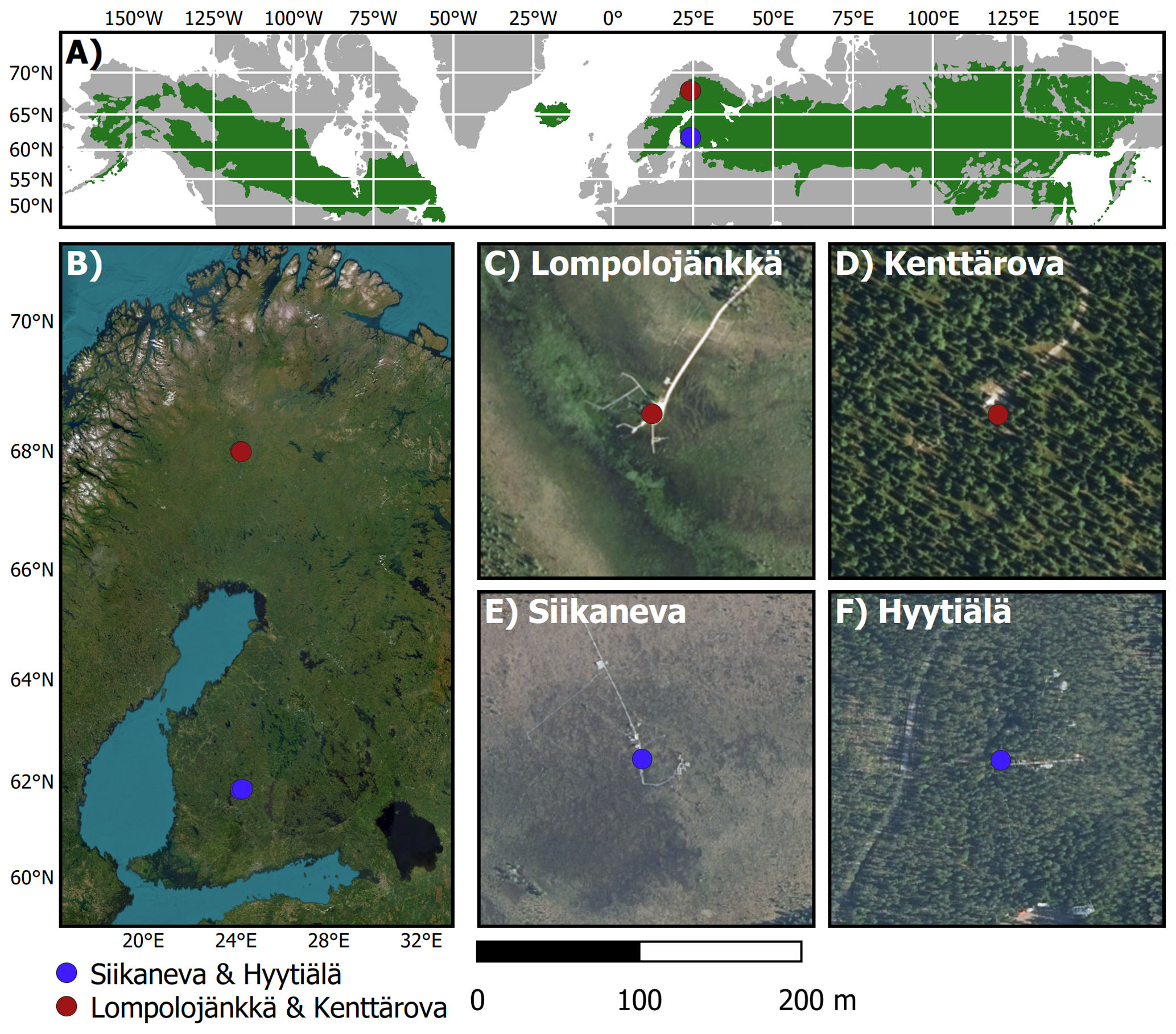
2.1.1 Pallas supersite (N-WET and N-FOR)

The Pallas area represents northern subarctic conditions and is characterized by pine and spruce forests, wetlands, fells, and lakes (Aurela et al., 2015; Lohila et al., 2015; Marttila et al., 2021). In this study, we use data from its two eddy-covariance (EC) flux stations.

Lompolojänkkä (northern peatland, N-WET) is a pristine northern boreal mesotrophic sedge fen where the wetter parts are dominated by sedges (Carex rostrata (most abundant), Carex chordorrhiza, Carex magellanica and Carex lasiocarpa) and the drier parts consist of shallow deciduous trees (Betula nana and Salix lapponum). Moreover, the fen has a fairly low coverage of shrubs, mainly Andromeda polyfolio and Vaccinium oxycoccos. The vegetation height is shallow (∼0.4 m), with the exception of isolated trees/bushes on the drier edges of the peatland.

Kenttärova (northern forest, N-FOR) is a northern boreal spruce forest, located on a hill-top plateau with mineral soil approximately 60 m above Lompolojänkkä wetland. The forest is dominated by Norway spruce (Picea abies) with some deciduous trees, mainly birch (Betula pubescens) but also aspen (Populus tremula) and pussy willow (Salix caprea). According to the classification by Brunet (2020), Kenttärova is a sparse forest. Both sites and their measurements have been described in detail by Aurela et al. (2015).

2.1.2 Hyytiälä and Siikaneva (S-WET and S-FOR)

The sites are located in southern subarctic conditions in the Pirkanmaa region in southern Finland, at about 5 km distance from each other. Siikaneva fen (southern wetland, S-WET) is a southern boreal oligotrophic fen dominated by sedges (Eriophorum vaginatum, Carex rostrata and Carex limos) and has an extensive Sphagnum cover (mainly Sphagnum balticum, Sphagnum majus and Sphagnum papillosum). The site has been described in detail in Aurela et al. (2007), Alekseychik et al. (2017) and Rinne et al. (2018).

Hyytiälä (southern forest, S-FOR) is a managed boreal Scots pine (Pinus sylvestris) dominated forest on mineral soil, described in detail by Launiainen (2010); Launiainen et al. (2022). According to the classification by Brunet (2020), the site is a dense forest.

Table 1 General site information.

2.2 Models

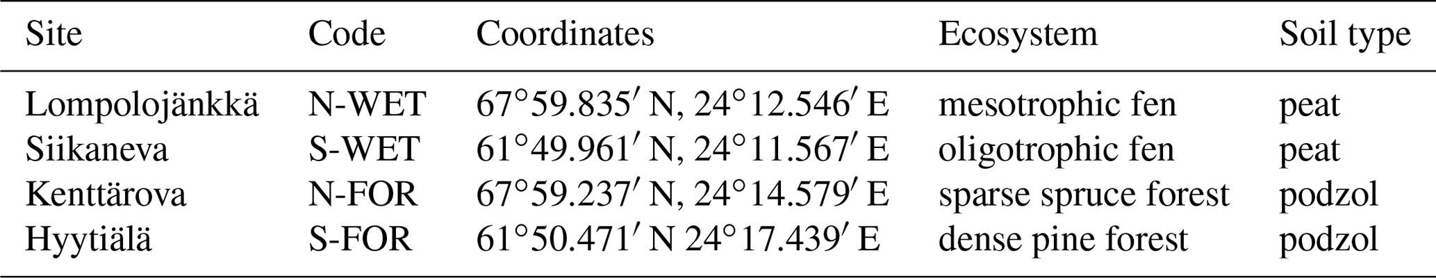
We use components from the SURFEX LSM (Surface Externalisée, Masson et al., 2013) platform. SURFEX was selected as its modularity and vast range of model structures and incorporated process parameterizations enable its use in diverse applications. Specifically, we used ISBA (Noilhan and Planton, 1989; Noilhan and Mahfouf, 1996) for composite soil–vegetation, MEB (Boone et al., 2017; Napoly et al., 2017) for the canopy and Crocus (Vionnet et al., 2012), and its ensemble/multiphysics version ESCROC (Lafaysse et al., 2017) for the snowpack simulations. Specifically, ISBA coupled to Crocus is used for both peatland and forest experiments (Fig. 2a, b), whereas MEB coupled to Crocus is only used for the forest experiments (Fig. 2c). In the next subsections, we briefly describe these model components. Parameterizations and different configurations of ISBA, MEB and Crocus models are detailed in Sect. 2.3.

2.2.1 ISBA

ISBA (Interactions between the Soil, Biosphere and Atmosphere) is the soil and vegetation component of SURFEX (Noilhan and Planton, 1989; Noilhan and Mahfouf, 1996). It simulates the mass and energy fluxes in the soil–vegetation composite, as well as the exchanges between the soil–vegetation and the overlying atmosphere/snowpack (Fig. 2a, b). ISBA is used for the general circulation models by Météo-France (Mahfouf et al., 1995; Douville et al., 1995; Salas-Mélia et al., 2005; Voldoire et al., 2013, 2019) and for numerical weather prediction in numerous countries (e.g., Hamdi et al., 2014; Bengtsson et al., 2017).

In ISBA, the surface heat flux between the atmosphere and the soil–vegetation composite (G₀, W m⁻²) is computed as the residual of the sum of all surface/atmosphere energy fluxes:

$$\begin{array}{}\text{(1)}& G_{\mathrm{0}}=\mathrm{SWD}(\mathrm{1}-\mathrm{LSA})+\mathit{ϵ}(\mathrm{LWD}-\mathit{\sigma }{T}_{\mathrm{s}}^{\mathrm{4}})+H+\mathrm{LE},\end{array}$$

where SWD (Wm⁻²) and LWD (Wm⁻²) are the incoming shortwave and longwave radiations, respectively. The land surface albedo is denoted as LSA, ϵ is the surface emissivity, σ is the Stefan–Boltzmann constant and T_s (K) is the surface temperature. The sum of the radiation terms is hereafter denoted as R_n (Wm⁻²).

The sensible heat flux H (Wm⁻²) is computed with the bulk aerodynamics approach:

$$\begin{array}{}\text{(2)}& H={\mathit{\rho }}_{\mathrm{a}}{c}_{\mathit{\rho }}{C}_{\mathrm{H}}{V}_{\mathrm{a}}(T_{\mathrm{s}}-T_{\mathrm{a}}),\end{array}$$

where the air density, the specific heat capacity, the wind speed and the air temperature are denoted with ρ_a (kg m⁻³), c_p (${\mathrm{Jkg}}^{-\mathrm{1}}{\mathrm{K}}^{-\mathrm{1}}$), V_a (ms⁻¹) and T_a (K), respectively. C_H is the turbulent exchange coefficient described later and is one of the parameters that is the focus of this study. When the soil is not fully covered by snow, the latent heat flux LE (Wm⁻²) is the sum of evaporation from the bare soil surface, E_g; evaporation of intercepted water on the canopy, E_c; transpiration from the vegetation, E_tr; and sublimation from bare soil ice, S_i:

$$\begin{array}{}\text{(3)}& \mathrm{LE}=L_{\mathrm{v}}(E_{\mathrm{g}}+E_{\mathrm{c}}+E_{\mathrm{tr}})+(L_{\mathrm{f}}+L_{\mathrm{v}})\left(S_{\mathrm{i}}\right),\end{array}$$

where L_v (Jkg⁻¹) and L_f (Jkg⁻¹) are the latent heat of vaporization and fusion, respectively. Total evapotranspiration (ET) is computed as

$$\begin{array}{}\text{(4)}& \begin{array}{rl}\mathrm{ET}& =E_{\mathrm{g}}+E_{\mathrm{c}}+E_{\mathrm{tr}}=(\mathrm{1}-\mathrm{veg}){\mathit{\rho }}_{\mathrm{a}}{C}_{\mathrm{H}}{V}_{\mathrm{a}}\\ & \left[h_u{q}_{\mathrm{sat}}\right(T_{\mathrm{s}})-q_{\mathrm{a}}]+\mathrm{veg}{\mathit{\rho }}_{\mathrm{a}}{C}_{\mathrm{H}}{V}_{\mathrm{a}}{h}_v,\end{array}\end{array}$$

where veg is the fraction of vegetation cover, q_sat(T_s) (kgkg⁻¹) is the saturated specific humidity at the surface, q_a(T_s) (kg kg⁻¹) is the atmospheric specific humidity, h_u is the dimensionless relative humidity at the ground surface related to the superficial soil moisture content, and h_v is the dimensionless Halstead coefficient describing the E_c and E_tr partitioning between the leaves covered and not covered by intercepted water (see Noilhan and Mahfouf (1996) for details)

The turbulent exchange coefficient C_H is based on the formulation of Louis (1979):

$$\begin{array}{}\text{(5)}& C_{\mathrm{H}}=\left[{\displaystyle \frac{k^{\mathrm{2}}}{\ln (z_u/z_{\mathrm{0}t})\ln (z_{\mathrm{a}}/z_{\mathrm{0}t})}}\right]f\left(Ri\right),\end{array}$$

where z_u (m) is the reference height of V_a, z_a (m) is the reference height of T_a and humidity, z_0t (m) is the roughness height for heat, k (–) is the von Kármán constant, and f(Ri) (–) describes the decrease in C_H as a function of increasing atmospheric stability, represented through Richardson number (Ri)  (Louis, 1979).

Instead of separate treatment of the vegetation canopy and ground, ISBA considers the composite soil–vegetation energy budget (Fig. 2a, b). In the most detailed soil scheme ISBA diffusion (ISBA-DIF, Boone et al., 2000; Decharme et al., 2011), used in this study, the 1D Fourier law is used to solve the soil heat diffusion, while a mixed-form Richards equation is applied for the 1D soil water movements. Similar to Napoly et al. (2020), we use the A−g_s stomatal conductance formulation derived from the coupling of photosynthetic CO₂ demand and stomatal function (Calvet et al., 1998).

ISBA uses parameters such as one-sided leaf area index (LAI, m² m⁻²), vegetation height, vegetation thermal inertia, albedos of soil and vegetation, fractions of sand and clay, and SOC content to characterize the composite soil–vegetation column. These parameters may be defined by the user or obtained from global or regional databases (e.g., Faroux et al., 2013) and pedotransfer functions (Noilhan and Mahfouf, 1996; Peters-Lidard et al., 1998). In the presence of full snow cover, the surface energy budget is solved by Crocus (Sect. 2.2.3). For partial snow cover, Crocus is used to solve the snow-covered fraction while the energy balance of the snow-free fraction is computed by ISBA, and total surface energy fluxes are computed as weighted averages of the snow and snow-free fractions (Sect. 2.3.1).

2.2.2 MEB

MEB (multi-energy balance) is a recent ISBA development to explicitly describe vegetation and soil energy and mass balances. It was developed initially for forests (Boone et al., 2017; Napoly et al., 2017) and found to yield improved snow and soil temperature simulations (Napoly et al., 2020) but has not been evaluated for boreal and subarctic conditions. MEB simulates surface energy budget separately for soil and vegetation canopy. When the ground is snow covered, the energy budget of the snowpack is also explicitly represented. We used the MEB option, where the forest floor is covered by a litter layer instead of the bare soil surface (Napoly et al., 2020) (Fig. 2c). MEB describes vegetation canopy as a single big leaf (Boone et al., 2017). The respective energy balance equations for the canopy, the snowpack and the ground surface/litter layer in MEB are

$$\begin{array}{}\text{(6)}& \left\{\begin{array}{l}{C}_{\mathrm{v}}\frac{\partial T_{\mathrm{v}}}{\partial t}=R_{\mathrm{nv}}-H_v-{\mathrm{LE}}_v+L_{\mathrm{f}}{\mathit{\varphi }}_v\\ C_{\mathrm{g},\mathrm{1}}\frac{\partial T_{\mathrm{g},\mathrm{1}}}{\partial t}=(\mathrm{1}-{\mathit{\rho }}_{\mathrm{sng}})(R_{\mathrm{ng}}-H_g-{\mathrm{LE}}_g)\\ +{\mathit{\rho }}_{\mathrm{sng}}(G_{\mathrm{gn}}+{\mathit{\tau }}_{n,Nn}{\mathrm{SW}}_{\mathrm{nn}})-G_{\mathrm{g},\mathrm{1}}+L_{\mathrm{f}}{\mathit{\varphi }}_{\mathrm{g},\mathrm{1}}\\ C_{\mathrm{n},\mathrm{1}}\frac{\partial T_{\mathrm{n},\mathrm{1}}}{\partial t}=R_{\mathrm{nn}}-H_n-{\mathrm{LE}}_n-{\mathit{\tau }}_{\mathrm{n},\mathrm{1}}{\mathrm{SW}}_{\mathrm{nn}}\\ +{\mathit{ϵ}}_{\mathrm{n},\mathrm{1}}-G_{\mathrm{n},\mathrm{1}}+L_{\mathrm{f}}{\mathit{\varphi }}_{\mathrm{n},\mathrm{1}}\end{array}\right.,\end{array}$$

where C_v, C_g,1, and C_n,1 (${\mathrm{Jm}}^{-\mathrm{2}}{\mathrm{K}}^{-\mathrm{1}}$) and T_v, T_g,1, and T_n,1 K are the effective heat capacities and temperatures of the canopy, ground surface/litter layer, and snowpack, respectively. In these equations, the subscripts g,1 and n,1 represent the uppermost layer for the soil and the snowpack, respectively. G_g,1 and G_n,1 are, respectively, the conduction heat flux at the bottom of the uppermost soil or snow layer. G_gn is the conduction heat flux at the soil–snow interface. R_nv, R_ng and R_nn (Wm⁻²) are net radiation, i.e., the sum of net shortwave radiation and net longwave radiation from/to the corresponding layer. The shortwave radiation scheme used in MEB is described in Carrer et al. (2013). Light transmission through the canopy is computed with a sky view factor, which depends on LAI, solar angle and a vegetation-dependent constant (see Eq. 45 in Boone et al., 2017). H and LE flux parameterization as well as the stability correction functions are detailed in Boone et al. (2017). Obviously T_v, T_g,1 and T_n,1 are also involved in the radiative and turbulent terms, providing a linear system of equations to be solved by an implicit numerical scheme. In this study, MEB is coupled to the ISBA-DIF soil scheme (Sect. 2.2.1) and the snowpack model Crocus (Sect. 2.2.3). Energy fluxes between the canopy and the ground surfaces are calculated within MEB and prescribed as upper-boundary conditions in the subsequent Crocus and ISBA-DIF calculations.

2.2.3 Crocus

Crocus is a 1D physically based multilayer snowpack model (Vionnet et al., 2012). It is the most detailed snow scheme in ISBA and has been used for operational avalanche hazard forecasting in the French mountain ranges for the past 3 decades (Morin et al., 2020). It aims to mimic the vertical layering of snowpacks with a Lagrangian discretization system, avoiding the aggregation of snow layers with highly different physical properties. A detailed description of Crocus and its integration in SURFEX can be found in Vionnet et al. (2012).

The snowpack surface energy budget is the sum of net radiation, turbulent fluxes and advective fluxes from precipitation. Over the snow, the sensible heat flux is computed similarly as in ISBA (Eq. 2) for soil surface, while the latent heat flux (sublimation/deposition), LE_s, is computed as

$$\begin{array}{}\text{(7)}& {\mathrm{LE}}_{\mathrm{s}}=(L_f+L_v){\mathit{\rho }}_a{C}_H{V}_{\mathrm{a}}\left[q_{\mathrm{sat}}\right(T_{\mathrm{s}}\mathrm{-}{q}_a\left)\right],\end{array}$$

where T_s (K) is the snow surface temperature. The bottom of the snowpack and the uppermost soil layer of ISBA are fully coupled with a mass- and energy-conserving semi-implicit solution. The semi-implicit solution refers to a coupled system in which both components are solved separately with an implicit approach considering that the state of the second system remains constant during the solving of the first system. The heat conduction flux G_gn at the snow–soil interface is explicitly computed using the Fourier equation and depends on the temperature gradient between the bottom snow layer and the uppermost soil layer (Eq. 4 in Decharme et al., 2011). The soil thermal conductivity and heat capacity are described using pedotransfer functions of ISBA (Noilhan and Mahfouf, 1996; Peters-Lidard et al., 1998).

2.3 Model configurations and parameterization

2.3.1 Model configurations

We use three different configurations of ISBA, MEB and Crocus modules (Fig. 2). The first two configurations use the composite soil–vegetation conceptualization of ISBA (Fig. 2a, b) and differ only in how the snow cover fraction is represented. ISBA aggregates the properties of soil and vegetation depending on vegetation fraction (veg) that covers a given grid cell.

The first configuration (referred to as ISBA-FS) assumes the snowpack fully covers the soil–vegetation composite regardless of the snow depth (Fig. 2a). It is the common approach for snow simulations over shallow vegetation or bare soil (Vernay et al., 2022; Nousu et al., 2019), for large-scale reanalyses (Brun et al., 2013), and for some hydrological applications (Lafaysse et al., 2011; Revuelto et al., 2018). In addition, most site-level evaluations of SURFEX snow schemes rely on ISBA-FS configuration (Decharme et al., 2016; Lafaysse et al., 2017).

In the second configuration (referred to as ISBA-VS), a part of the soil–vegetation composite is covered by snow while the remaining (non-snow) fraction stays in constant contact with the atmosphere. This proportion is governed by snow depth. The effective snow cover fraction is the weighted average between the snow fraction of vegetation (p_snv) and snow fraction of the bare ground (p_sng), calculated as (Decharme et al., 2019; Napoly et al., 2020)

$$\begin{array}{}\text{(8)}& p_{\mathrm{snv}}=min\left(\mathrm{1.0},{\displaystyle \frac{\mathrm{HS}}{\mathrm{HS}+w_{\mathrm{sw}}{z}_{\mathrm{0}}}}\right),\end{array}$$

$$\begin{array}{}\text{(9)}& p_{\mathrm{sng}}=min\left(\mathrm{1.0},{\displaystyle \frac{\mathrm{HS}}{{\mathrm{HS}}_g}}\right),\end{array}$$

where HS (m) is the snow depth, HS_g is the threshold value for snow depth (0.01 m by default) and z₀ (m) denotes the surface roughness. The coefficient w_sw is supposed to relate to scale-dependent vegetation characteristics and is set to 5 by default in SURFEX and in numerical weather prediction configurations (as well as in this study). However, without clear consistency, highly different values of w_sw have been used, e.g., in climate simulations (w_sw=2 by Decharme et al., 2019) and hydrological applications (w_sw=0.2 by Le Moigne et al., 2020). We present a summary of the application-specific treatment of the snow cover fraction and w_sw in the Appendix (Table C1). This summary shows that selection of the w_sw value seems arbitrary and the fractional concept is only loosely linked to any physical relationships between soil, vegetation and snow. Yet, it is necessary for such a composite approach.

The third configuration (later denoted as MEB) is the big-leaf approach where the fluxes between the canopy and snowpack/ground are explicitly computed by MEB and prescribed in the subsequent Crocus snowpack and ISBA-DIF soil modules (Fig. 2c).

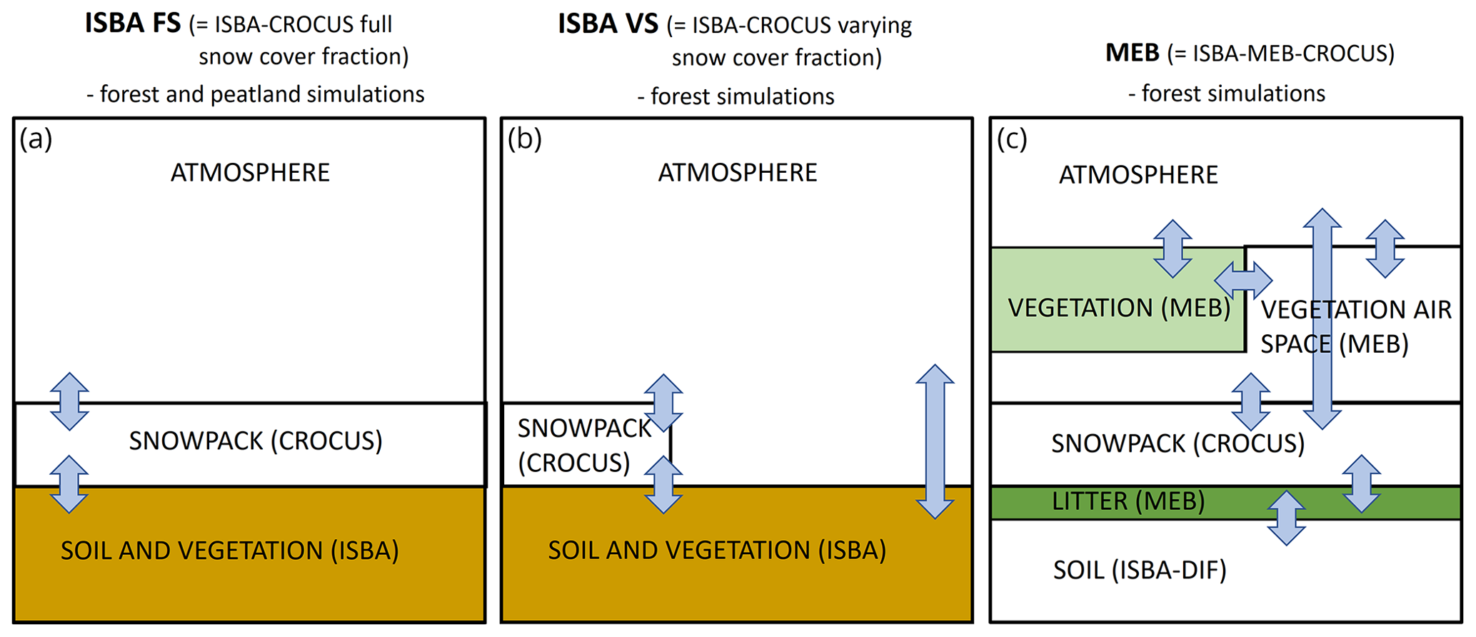
Figure 2 Three different model configurations used in the study: (a) ISBA-FS with full snow cover fraction, (b) ISBA-VS with varying snow cover fraction and (c) MEB big-leaf approach. Considered energy fluxes between domains are represented with arrows.

2.3.2 ESCROC parameterizations for snow processes and turbulent exchange

We use the multiphysics version of Crocus (ESCROC, Ensemble System Crocus, Lafaysse et al., 2017) to evaluate the impact and associated uncertainties of the different parameterizations of snow processes and turbulent exchange. In ESCROC, the main physical processes and properties of snowpack, as well as the turbulent fluxes, can be represented by several alternative options. These include density of new snow, snow metamorphism, absorption of solar radiation, turbulent fluxes, thermal conductivity, liquid water holding capacity, snow compaction and surface heat capacity (Eqs. 1–17 in Lafaysse et al., 2017). Lafaysse et al. (2017) showed that an optimized standard subensemble of 35 members (E₂ subensemble) is sufficient to provide a spread of the appropriate magnitude compared to model errors. We use this subensemble (hereafter ESCROC-E₂) similar to recent studies quantifying the model uncertainty (e.g., Deschamps-Berger et al., 2022; Tuzet et al., 2020). The presented ensemble spread corresponds to simulated values between ensemble minimum and maximum.

In Crocus, the default turbulent exchange parameterization (Eq. 5) has been found to underestimate the turbulent fluxes under stable conditions (Martin and Lejeune, 1998). Therefore, different stability dependencies of the C_H have been implemented in ESCROC-E₂. They differ mainly in the Ri thresholds below which C_H is assigned a constant value to enable turbulent heat and mass transport under stable conditions. As shown by Fig. 4 in Lafaysse et al. (2017), these parameterizations are the (a) classical Louis (1979) formula (later referred to as RIL) with threshold at Ri=0.2; (b) RIL with threshold at R_i = 0.1 (RI1); (c) RIL with threshold at Ri=0.026 (RI2); and (d) modified formulation with effective roughness length for heat (10⁻³ m), with minimum wind speed (0.3 ms⁻¹), and with threshold at Ri=0.026 (M98) by Martin and Lejeune (1998). The RIL parameterization is widely used in SURFEX applications (e.g., Decharme et al., 2019; Le Moigne et al., 2020), RI2 is applied in operational snow modeling in the Alpine area (Vernay et al., 2022) and M98 was recently used in the Canadian Arctic by Lackner et al. (2022). However, evaluations of the different Crocus turbulent flux parameterizations against surface flux data are still lacking. MEB uses a different stability correction term (Boone et al., 2017) and applies only the RIL option for the stable conditions.

2.3.3 Site parameters

The parameterization of ISBA and MEB for the study sites is given in Table 2. Summer LAI and vegetation height were obtained from literature, while winter LAI (and monthly LAI cycle) was estimated according to the proportion of deciduous and coniferous vegetation on each site. The LAI of S-FOR refers to conditions before forest thinning in early 2020. The thinning, resulting in ca. 35 % reduction in LAI, was neglected in our simulations as major part of the simulation period covers time before the thinning. Vegetation types in ISBA are characterized according to ECOCLIMAP (Champeaux et al., 2005); the forest sites in this study classify as boreal needleleaf evergreen, while the peatland sites are best represented as boreal grass. Additional parameters based on LAI, vegetation height and vegetation type are computed following the standard methods of ISBA (Noilhan and Mahfouf, 1996; Carrer et al., 2013).

Soil texture (sand and clay fractions) for the forest sites is based on in situ measurements. The peat soils at S-WET and N-WET were parameterized as fully organic for the uppermost 1 m, in accordance with field measurements (Väliranta and Mathijssen, 2021; Muhic et al., 2023), while the deeper layers were assigned as mineral soil similar to the contiguous forests. Although peat profiles may be deeper, the soils below the damping depth of annual temperature fluctuations (ca. 1.1 m for saturated peat soil with porosity ca. 90 %) are assumed not to have significant impact on surface energy flux dynamics. The SOC values for mineral soils of N-FOR and S-FOR were taken from Lindroos et al. (2022). The rest of the parameters presented in Table 2 were assigned as estimates. The thermal and water retention parameters are subsequently derived from the pedotransfer functions of ISBA (Noilhan and Mahfouf, 1996; Peters-Lidard et al., 1998).

Champeaux et al. (2005)Champeaux et al. (2005)Aurela et al. (2015); Alekseychik et al. (2017)Kolari et al. (2022)Aurela et al. (2015); Alekseychik et al. (2017)Kolari et al. (2022)FMI (2021)Aurela et al. (2015); Mammarella et al. (2019)Alekseychik et al. (2022a)Hari et al. (2013); Alekseychik et al. (2022a)FMI (2021)Lindroos et al. (2022)Muhic et al. (2023)Väliranta and Mathijssen (2021)Lindroos et al. (2022)Muhic et al. (2023)Väliranta and Mathijssen (2021)Väliranta and Mathijssen (2021)Muhic et al. (2023)

Table 2 Main model parameters for the study sites. Vegetation types BOGR and BONE correspond to boreal grass and boreal needleleaf evergreen, respectively.

2.4 Data

2.4.1 Model forcing

Meteorological forcing consist of hourly observations of air temperature, wind speed, precipitation rate, air humidity, downward shortwave and longwave radiation, and atmospheric pressure. The available meteorological observations from the nearest meteorological stations were obtained from Finnish Meteorological Institute (FMI) open database (FMI, 2021) (station IDs: N-WET 778135, N-FOR 101317, S-FOR 101987). Meteorological observations at the S-WET site come from the SMEAR database (Alekseychik et al., 2022a). At S-WET and S-FOR the shortwave and longwave radiation were obtained from the SMEAR database, while at N-WET and N-FOR data from FMI stations were used. The diffuse-to-total-shortwave-radiation ratio, r, was estimated as a function of the cosine of the sun zenith angle, μ. More specifically, a third-degree polynomial fit between r and μ was obtained using the atmospheric model SBDART (Ricchiazzi et al., 1998) to simulate diffuse and total solar radiation in clear-sky conditions. The atmospheric profile was set to typical winter conditions, 0.09 for the aerosol optical thickness, 300 DU for the ozone column and 0.854 g cm⁻² for the water vapor column.

The data gaps in meteorological observations were first filled by the contiguous sites (e.g., N-FOR for N-WET and vice versa) and the remaining gaps by other nearby meteorological stations (IDs: N-WET/N-FOR 101932, S-WET/S-FOR 101520). The missing radiation observations were first filled by the contiguous sites, and the remaining gaps by ERA5 reanalysis data (Hersbach et al., 2020). Only less than 10 h of ERA5 data was used for N-WET, N-FOR and S-WET. However, S-FOR radiation observations contained more gaps, specifically LWD in 2008–2012. A good agreement between site observations and ERA5 estimates of LWD is shown in the Appendix (Fig. B1). Furthermore, the fraction of snow to total precipitation $P_{\mathrm{ice}}/(P_{\mathrm{ice}}+P_{\mathrm{liq}}$) is assumed to linearly decrease from 1 to 0 at air temperatures between 0 and 1 ^∘C.

2.4.2 Model evaluation data

We use surface energy flux observations, snow depth and soil temperatures in model evaluation. The availability period of each variable is given in Table B1. On all sites, upward shortwave radiation (SWU) and upward longwave radiation (LWU) were measured using pyranometers and pyrgeometers, while ground heat flux (G) was measured using soil heat flux plates between 5 and 10 cm depths.

The sensible heat (H) and latent heat (LE) were measured by the eddy-covariance (EC) technique. The EC systems consist of USA-1 (METEK) three-axis and Gill HS-50 sonic anemometers as well as closed-path LI-7000 and LI-7200 (LI-COR, Inc.) CO₂/H₂O analyzers. The detailed descriptions of the instrumentation, footprint analysis and the procedures for obtaining the turbulent heat fluxes from raw eddy-covariance data are detailed in the original data and site publications (N-WET/N-FOR, Aurela et al., 2015; and S-WET/S-FOR, Mammarella et al., 2016, 2019; Alekseychik et al., 2022b). In short, H and LE were screened for instrument failure and data outliers, and data were quality flagged according to friction velocity (u_*) and flux stationarity (FST) criteria (Foken et al., 2005) as follows

• flag 2: all data (after screening of instrument failures and outliers);

• flag 1: $u_{*}\ge \mathrm{0.1}$ ms⁻¹ and 0.3≤ FST ≤1.0;

• flag 0: $u_{*}\ge \mathrm{0.1}$ ms⁻¹ and FST ≤0.3.

At S-WET, S-FOR and N-FOR, automated snow depth observations are directly used (FMI, 2021). On N-WET the automated snow depth measurement is at 0.7 m height, and therefore the exceeding snow depths were taken from biweekly manual measurements. To account for the spatial variability of snow depth in the forests, manual snow depth measurements from a snow course in close proximity of the automated measurements were used (Aalto et al., 2022; Marttila et al., 2021). Each site has different configuration of soil temperature sensors. At N-FOR and N-WET stations, soil temperatures are measured at 5 and 20 cm depths (Aurela et al., 2015). Soil temperatures at S-FOR and S-WET are measured at depths of 0, 5, 10, 30, 50 and 75 cm (Aalto et al., 2022).

2.5 Model experiments

On the peatland sites, we evaluate the skill of ISBA-FS (Sect. 2.3.1) and effect of ESCROC-E₂ parameterizations (Sect. 2.3.2) on surface heat fluxes over snowpack and bare ground. The simulations are further used to assess the differences in snow depth simulations between ESCROC-E₂ turbulent exchange options. For a more detailed evaluation of two contrasting turbulent exchange options, we conducted deterministic ISBA-FS simulations with site parameters and default ESCROC-E₂ snow parameterizations but different treatments of turbulent exchange, RIL and M98 options (see Sect. 2.3.2; referred to as RIL-SOC and M98-SOC). Moreover, the influence of soil texture was explored by comparing M98-SOC to the simulation where soil was parameterized as mineral soil, similar to the contiguous forest site (referred to as M98-MIN).

On the forest sites, we examine the skills of the different alternatives to represent the energy and mass budgets of soil and vegetation (ISBA-VS, ISBA-FS, and MEB in Sect. 2.3.1), as well as their implications on snow depth, soil temperature and surface energy fluxes. First, we compare ESCROC-E₂ simulations with these three configurations focusing on the snow depth and soil temperature. These ISBA-VS simulations are conducted with the default snow cover fraction parameterization (w_sw=5 in Eq. 8). Additional ISBA-VS simulations are performed to assess the sensitivity of the w_sw parameter, using a value of 0.2 in Eq. (8). For a more detailed comparison of the simulated and observed above-canopy surface energy fluxes, we conduct deterministic simulations with both ISBA-VS and MEB, the default snow cover fraction and Crocus parameterizations (as in Fig. 2. in Lafaysse et al. (2017)). Additionally, we perform a deterministic ISBA-VS simulation with the default snow cover fraction parameterization but the vegetation fraction set to unity.

Model simulation periods for each site are in Table 2. For each site, the model initial state was obtained by a spin-up simulation from the start date (Table 2) to September 2020. A total of 361 ensemble and deterministic simulations were conducted.

2.6 Model evaluation metrics

Time series of daily averages are used to represent the results, whereas mean absolute error (MAE), mean bias error (MBE) and coefficient of determination (R²) are used in quantitative model–data comparison. To detect possible biases in model simulations, we use scatterplots and quantile–quantile plots of sorted observations against sorted simulations. The sign convention is so that the surface energy fluxes are presented relative to the surface (i.e., negative flux means that surface is losing energy). In time series, the turbulent flux observations include all EC data (Sect. 2.4.2, quality flag ≤2). We demonstrate the results by using the winter season 2018–2019 as an example time series period thanks to its best coverage of energy flux data (least gaps) and typical snow conditions on all sites. For the scatter and quantile–quantile plots, only flux data with quality flag ≤1 are used, and the results computed as aggregated 6 h means include periods where observations are available (referred to later as evaluation period). We compare snow and snow-free conditions by grouping the results into time windows where models and observations agree of the ground conditions (snow or snow-free).

3 Results

3.1 Observed energy balance at peatland and forest sites

The energy budget at high latitudes has a strong seasonal variation driven by solar radiation (Fig. 3). In winter (December, January, February), longwave radiation balance to a large extent determines R_n, particularly in northern Finland. Daily average R_n is negative down to −50 Wm⁻² and lower, which implies considerable radiative cooling. Towards spring the radiation budget is gradually counterbalanced by shortwave radiation. On the peatlands, a large fraction of SWD is reflected during snow cover, and daily R_n turns positive in the late melting season (Fig. 3a, c). At the forest sites, the timing of R_n becoming positive is less sensitive to the presence of snow, as a large proportion of SWD is absorbed by vegetation. In summer, high solar elevation and the absence of the reflective snow surface cause daily R_n to be up to 200 Wm⁻².

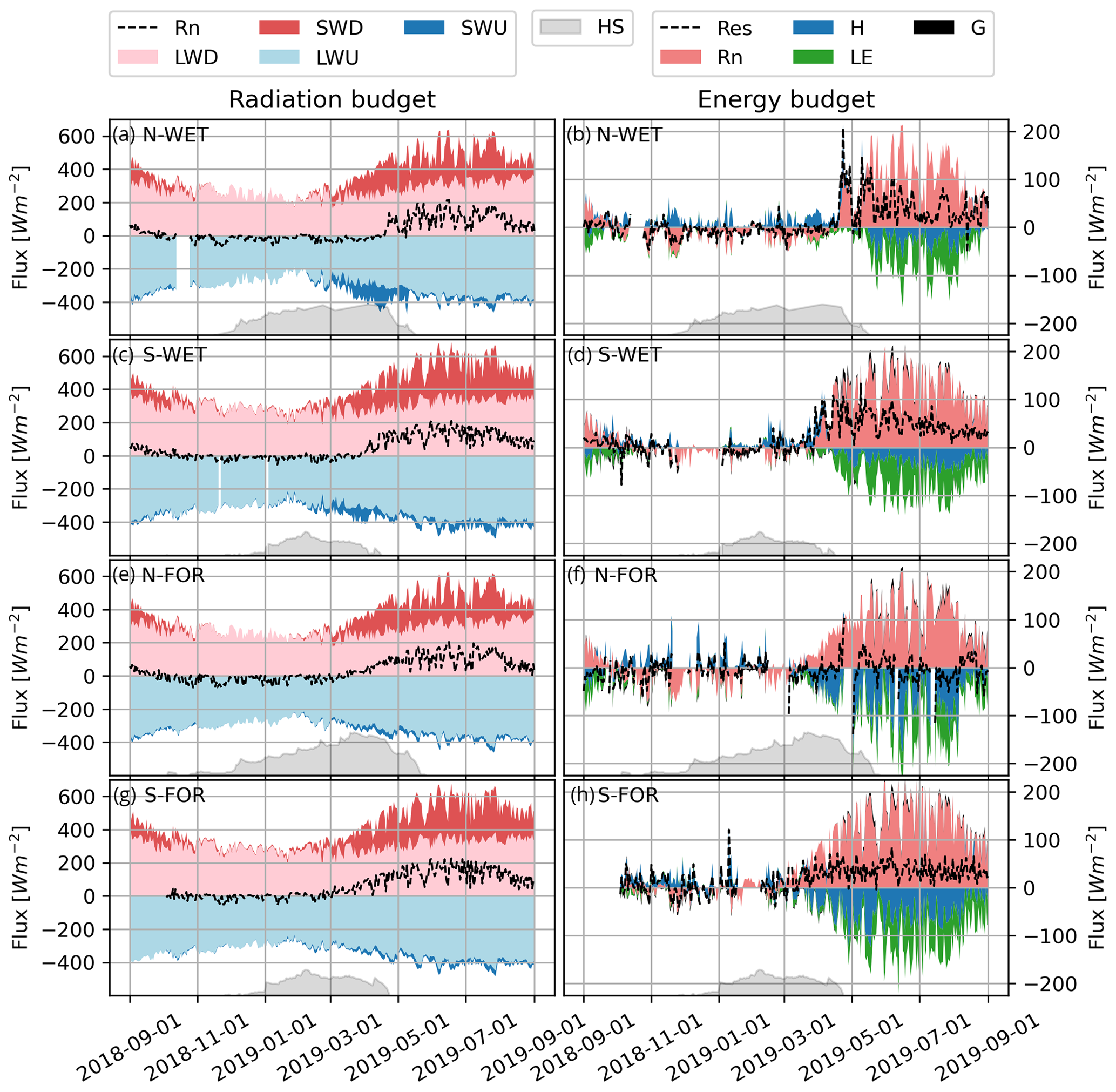
Figure 3 Observed daily averaged radiation budget (a, c, e, g) and surface energy budget (b, d, f, h) of hydrological year of 2018–2019. Colored stacks represent the observed fluxes relative to the surface as shown in legends (i.e., incoming fluxes are positive and outgoing fluxes negative). The dashed line in the energy budget plot corresponds to the residual after the sum of each energy component, whereas the dashed line in the radiation plot shows the net radiation (R_n). Note the different scale in the left and right columns. Ground heat flux (G) is missing on N-WET. The observed evolution of the snow depth (HS) is shown in gray (not to scale).

R_n is balanced mostly by H and LE and to a lesser extent snowpack–ground heat flux (Fig. 3). The residual line represents the amount of energy that would be required to close the observed energy budget (Fig. 3). It includes changes in internal energy of the snowpack and vegetation but also reflects the common energy balance closure problem in EC measurements (Mauder et al., 2020) (see Sect. 4.4). The energy balance closure in snow-free conditions was typical for EC measurements, ranging from 0.81 to 0.99 (Mauder et al., 2020). The lack of snowpack heat flux and/or temperature profile measurements did not enable assessing the closure during snow cover periods. In winter, LE and G are small and the radiative cooling is counterbalanced mostly by downward H, corresponding to warming of the snowpack and/or vegetation and cooling of the ambient air. R_n during winter falls lower (more negative) on the northern sites, and thus also downward H becomes stronger (daily average up to 50 Wm⁻²). In summer, both H and LE are negative (upward), heating the atmosphere, while downward G drives the warming of soil profile. At all sites, LE increases along the growing season and peaks approximately in July. In autumn, the turbulent fluxes decrease in response to reduced R_n.

3.2 Peatland simulations

The sensitivity of surface heat fluxes and snow depth to different ESCROC-E₂ model parameterizations is shown in Fig. 4. The spread corresponds to the difference between the minimum and maximum of the ensemble. Notably, H has relatively high spread, especially on N-WET, and the observed H often lies near the limit or even outside the simulated range at both S-WET and N-WET. Modeled wintertime LE is low and, as for H, the observed values are near the limit or outside the simulated range, especially in spring. LWU has strong day-to-day variation well captured by the model, and the spread is rather small relative to the total flux.

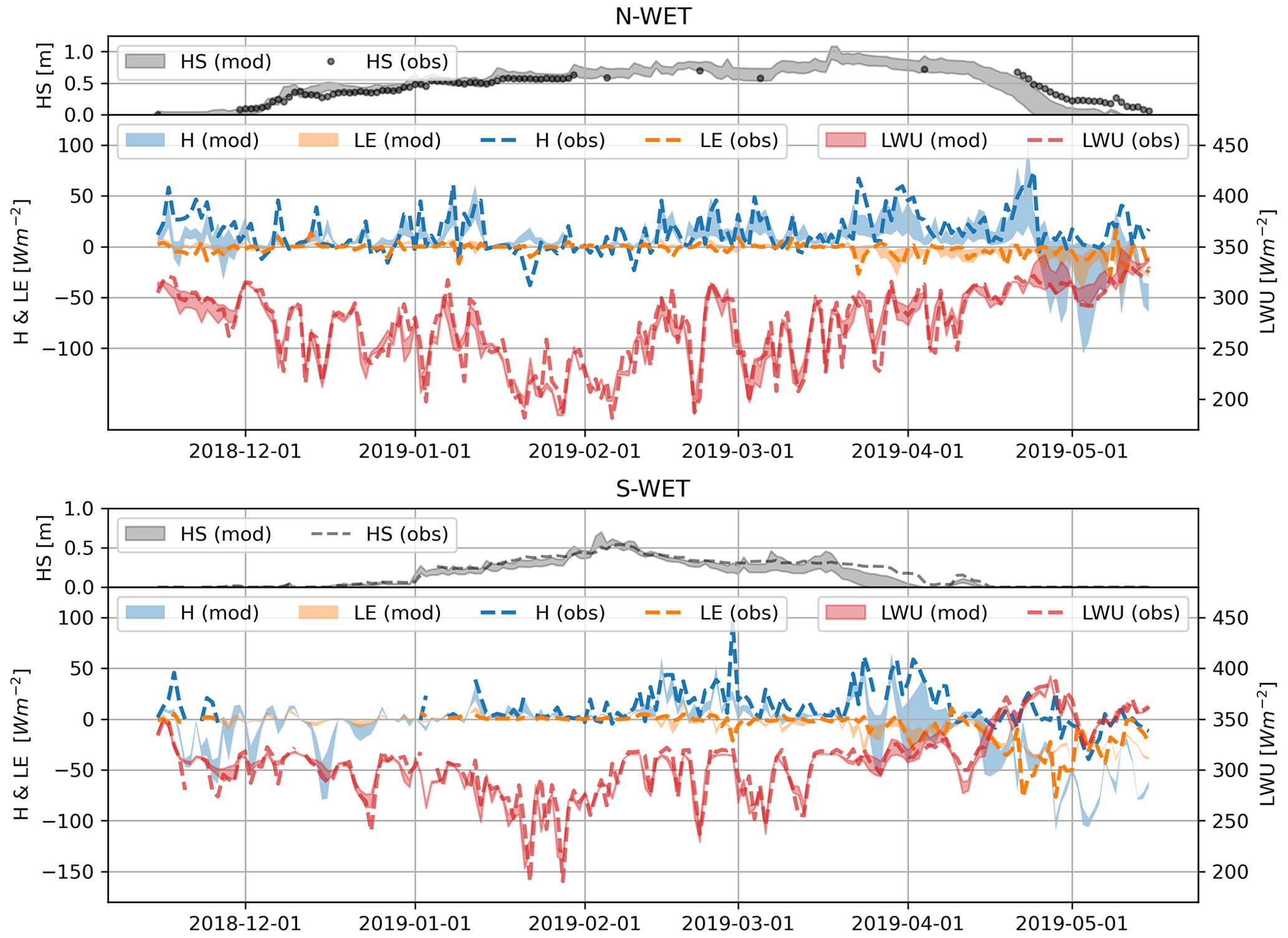
Figure 4 Time series of daily averaged surface heat flux spread simulated by ISBA-FS with ESCROC-E₂ 35 ensemble members against corresponding observed values during the 2018–2019 snow season. H, LE and LWU correspond to sensible heat, latent heat and upward longwave radiation fluxes, respectively. The observed and simulated evolution of snow depth (HS) are shown in gray.

3.2.1 Impact of alternative turbulence (C_H) parameterizations

To assess the sensitivity of snow depth simulations to alternative turbulence parameterizations and to alternative snow process options, we examined simulations where the ESCROC-E₂ members are grouped according to their turbulent flux option (Fig. 5). During snow accumulation periods, the spread is small and the groups are consistently overlapping on both sites, indicating that the differences in snow accumulation and maximum snow depth are driven mostly by the uncertainty of snow process descriptions. The spread increases during and after snowmelt events, indicating higher importance of turbulent fluxes on snowmelt dynamics. While it is difficult to identify a group that fits observed snow depths best, the winter melt event in 2018–2019 on N-WET is only captured by the M98 and RI2 parameterizations.

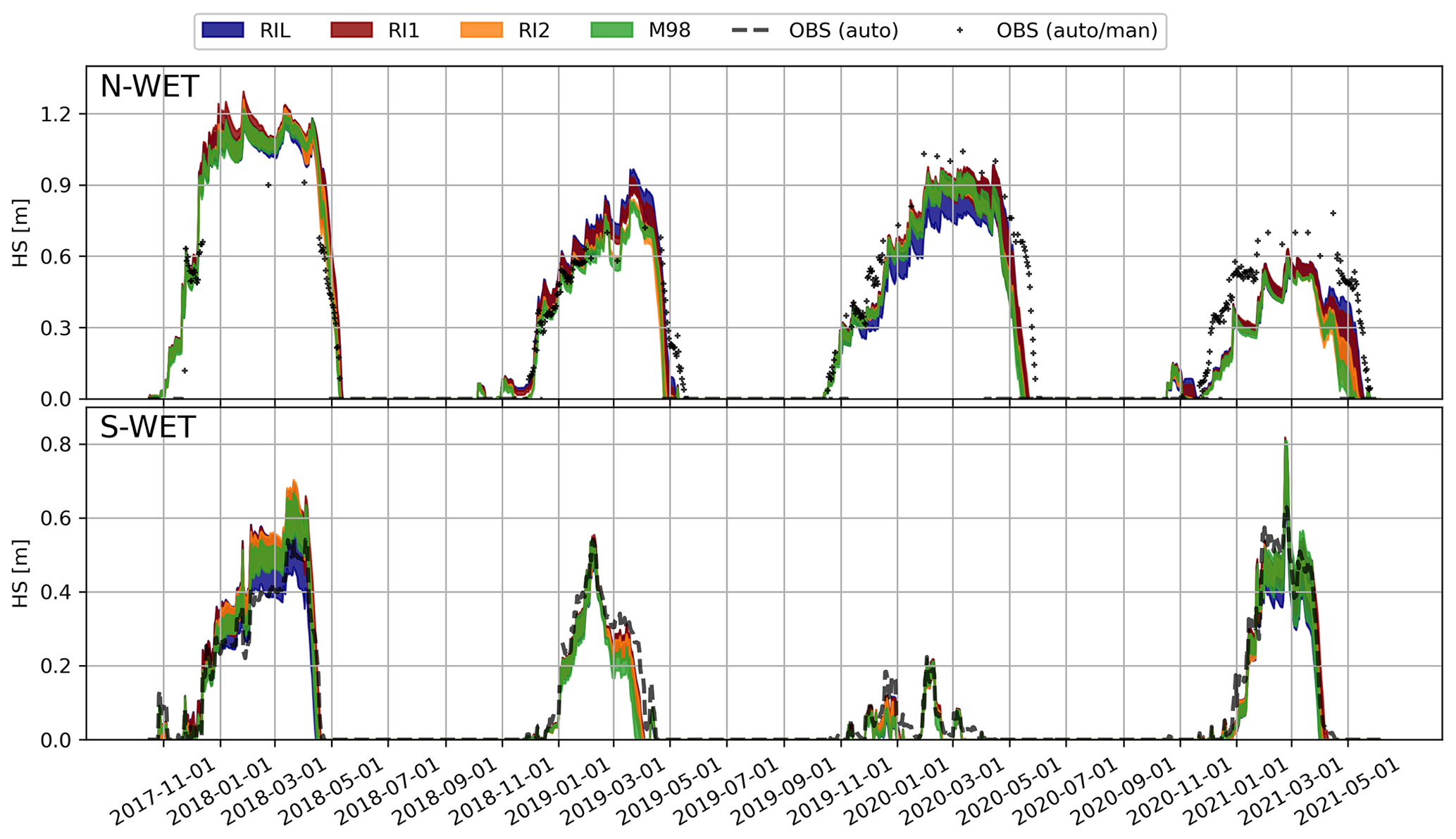
Figure 5 Time series of snow depths (HS) simulated by ISBA-FS ESCROC-E₂. The 35 ensemble members are grouped by their turbulent flux parameterization, and the spread of each group is presented in colored ranges. Observed snow depths are presented in black dots and dashed lines.

These findings are consistent with the comparison of simulated H and LWU by the two deterministic runs (RIL-SOC and M98-SOC) against observations (Fig. 6). With the RIL-SOC parameterization, the magnitude of H is largely underestimated, while this bias is to a large extent corrected by using M98-SOC. Improved simulation of H and surface temperature also entail improved LWU (Fig. 6), but the modeled H fluxes still only moderately correlate (R²) with observations. In terms of LE, the simulations are not improved by the M98-SOC (see Fig. S1), possibly due to low magnitude and high relative uncertainty of wintertime LE over snow.

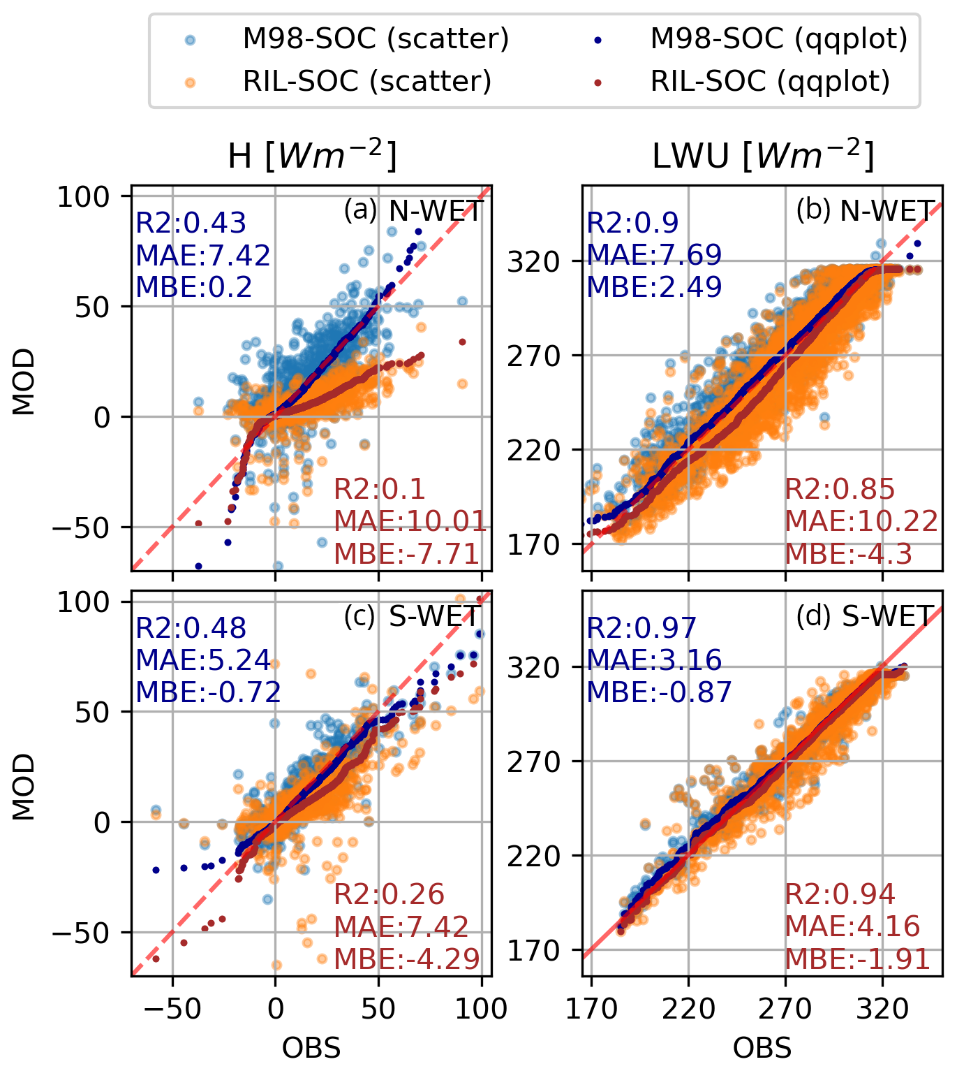
Figure 6 Scatterplots and quantile–quantile plots of sensible heat flux (H) and upward longwave radiation (LWU) during snow cover for the evaluation period with the RIL-SOC and M98-SOC turbulence parameterizations.

3.2.2 Radiative fluxes

We compare the simulated and observed albedo, SWU, LWU and surface temperatures with snow-free and snow conditions in Fig. 7. These experiments correspond to the deterministic M98-SOC simulation.

The modeled SWU generally matches the observations well, but the scatter increases with increasing SWD, indicating uncertainties in simulated albedo when shortwave forcing is high over the snowpack in spring. These cause a slight underestimation of simulated spring albedo, also visible in the time series especially on N-WET (Fig. 7). Moreover, simulated albedo tends to be overestimated during shallow snow depth both in spring and autumn. This is because the ISBA-FS approach assumes snow to completely cover the ground regardless of the snow depth, while in reality the fractional snow cover can lower the albedo. In contrast in May 2019, the underestimation of albedo on N-WET is due to an incorrect timing of snowmelt (too early snow disappearance in the simulation). The mean absolute errors in simulating SWU are small and of similar magnitude (from ∼4 to 9 Wm⁻²) both for snow and snow-free conditions.

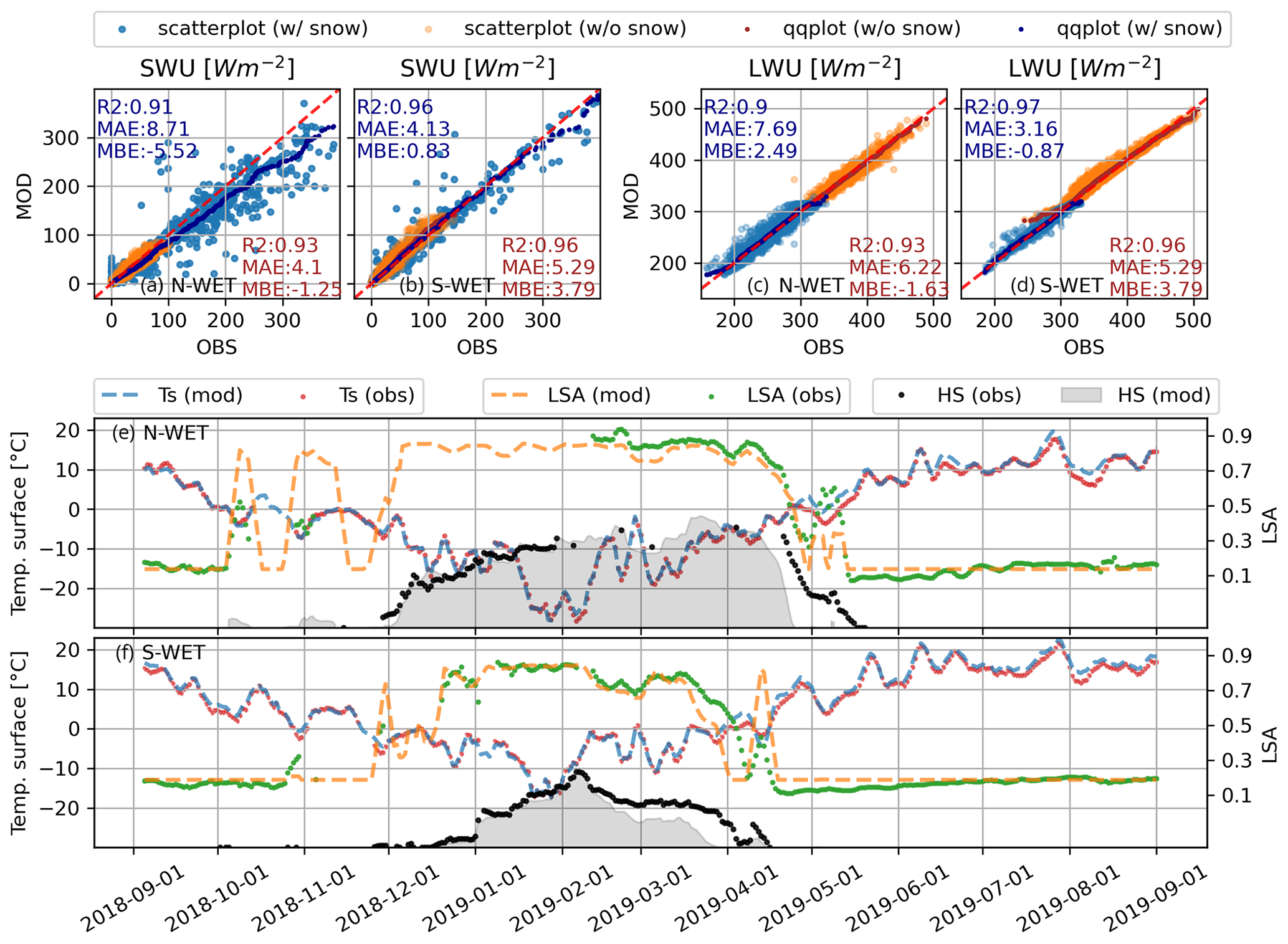
Figure 7 Scatterplots and quantile–quantile plots of modeled against observed upward shortwave radiation (SWU) (a, b) and upward longwave radiation (LWU) (c, d) on peatland sites with snow cover (w/ snow) and without snow cover (w/o snow) as well as the time evolution of 5 d rolling means of albedos (LSA) and surface temperature (T_s) as simulated and observed from September 2018 to September 2019 (e, f). The evolution of the snow depth (HS) is not to scale.

Warmer surface temperatures during the snow-free season result in higher LWU compared to winter and spring (Fig. 7). The surface temperatures and LWU are generally well simulated across sites and ground conditions at least with the presented time intervals. During snow cover, the upper tail of the radiation distribution is slightly higher than simulated; however, the mean biases are generally very low. There are no other visible biases in LWU simulations and the other metrics are also very good, consistent with Fig. 4. The mean absolute errors in simulating LWU are similar for snow and bare ground (∼3 to 8 Wm⁻²).

3.2.3 Soil thermal regime

The effect of soil parameterization on simulated soil temperature dynamics at S-WET is shown in Fig. 8. Due to shallow water table, the soil profile remains nearly saturated throughout the year. As the porosity and field capacity in the M98-SOC parameterization are much higher than in the M98-MIN, the former also has significantly higher heat capacity and smaller thermal diffusivity. This means soil temperature variations are attenuated in M98-SOC compared to M98-MIN, and this attenuation becomes increasingly important in deeper soil layers (Fig. 8). The results show that including a realistic soil profile (SOC) greatly improves the peatland soil temperature simulations at depths 50–70 cm but only slightly close to the surface (0–10 cm) (see Fig. S2 for comparisons of more soil depths). On both sites, the simulated surface soil temperature variations in summer are greater than observed. This is presumably because ISBA does not include the insulating moss/litter layer on top of the peat soil, as well as due to water table dynamics, potentially affected by lateral flows not accounted for. Due to the weak influence on the surface soil temperatures, the soil parameterization (M98-SOC vs. M98-MIN) does not significantly affect the simulated snow depth (Fig. S2).

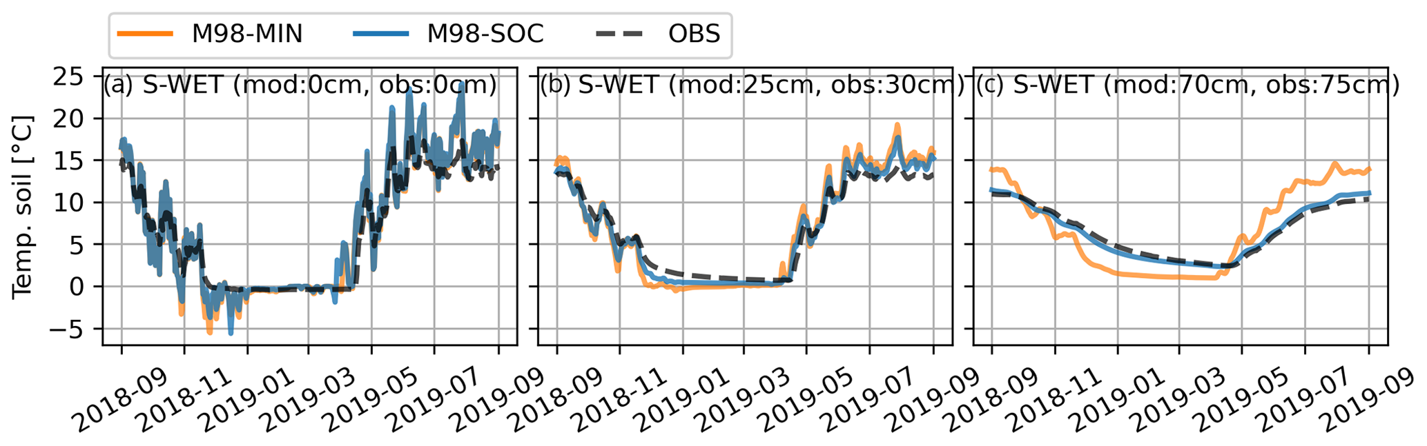
Figure 8 Effect of soil parameterization on soil temperatures (a–c) during a hydrological year at the S-WET site. M98-MIN refers to mineral soil and M98-SOC to peat soil. The observed soil temperatures are compared to the closest model layer; the depths of measurements and simulations are presented in each panel.

3.3 Forest simulations

3.3.1 Impact of vegetation representation on snow depth

The three different vegetation representations (Sect. 2.3.1) have a highly contrasting effect on the forest energy budget, snowpack and soil temperature simulations. In general, the snowpack simulations for the forest sites are poorer than for the peatland sites; however, the observed snow depths also vary considerably within the forests (see OBS in Fig. 9 and Sect. 4.4).

The simulated snow depth with the ISBA-VS (composite soil–vegetation and varying snow cover fraction, Fig. 2b) does not agree with the observations; the model version heavily overestimates accumulation on N-FOR in 2021 and predicts extremely rapid, strong and too early melt events (Fig. 9). Replacing the default snow cover fraction parameter (w_sw=5) with w_sw=0.2 (used for hydrological modeling in Le Moigne et al., 2020) yields slightly better snow depth dynamics for N-FOR, but the results remain unsatisfactory (Fig. C1 in the Appendix). The different sensitivity of the w_sw parameter for S-FOR and N-FOR simulations is explored via soil temperature simulations in Fig. C2; with the default snow cover fraction parameter, particular warm events on N-FOR heat up the soil, causing the snowpack to melt, while simulation with w_sw=0.2 manages to retain freezing soil temperatures.

MEB (explicit canopy, ground and snowpack energy balance) simulates the snow accumulation periods at N-FOR very well, but peak snow is reached too early, and maximum snow depths are underestimated. This is due to the combined impact of overestimated compaction and too early start and progression of the snowmelt. The role of both processes was evident from the comparison of modeled and observed snow water equivalent (see Fig. S6).

ISBA-FS performs better during the snow accumulation period, with simulated snow depths very close to observations. However, the ablation of snow is too rapid, and the final melt-out dates are close to those simulated by MEB. On S-FOR, MEB captures snow accumulation (including peak snow depths), melt dynamics and final melt-out dates rather well. ISBA-FS predictions are generally close to MEB. As MEB only considers one option for turbulent exchange (RIL), the spread of the ensemble is smaller than for the ISBA configurations (Fig. 9). The uncertainties of other snow processes accounted for in ESCROC-E₂ are not sufficient to explain the discrepancies between simulated and observed snow depths, suggesting that uncertainties in the canopy process representations prevail in these simulations.

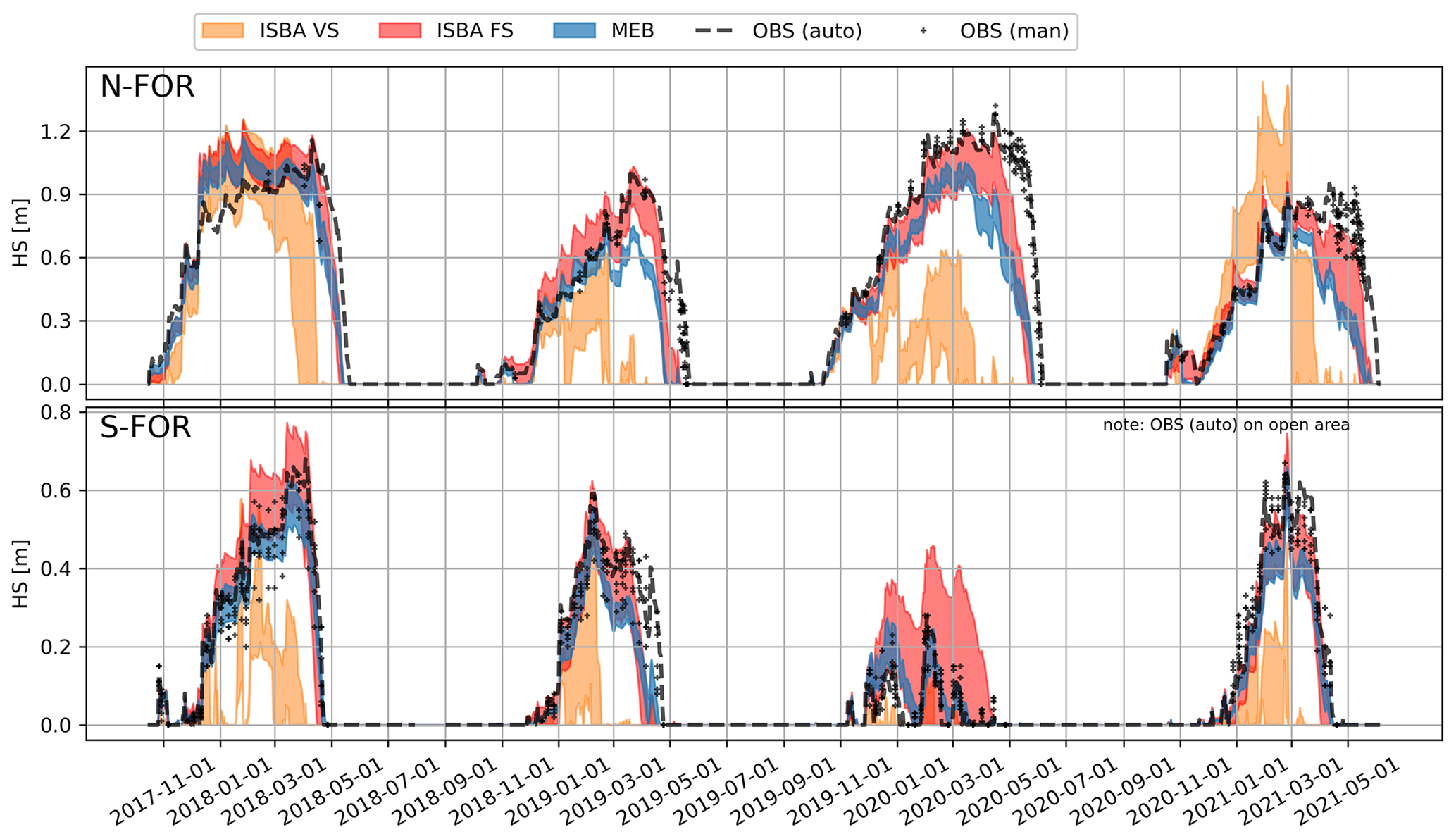
Figure 9 Effect of alternative configurations of ISBA and MEB on the snow depth (HS). The envelopes visualize the corresponding ensemble spreads between minimum and maximum values.

3.3.2 Impact of vegetation representation on soil temperature

Similar to the snow depth, soil temperature predictions by ISBA-VS are erroneous, with drastically underestimated temperatures and unrealistic dynamics (Fig. 10) (see more soil depths in Fig. S3). While MEB and ISBA-FS provided very similar snow depth, the soil temperatures simulated by MEB agree better with the observations, although there is a cold bias in autumn and a warm bias in summer (Fig. 10). On N-FOR the warm bias in winter by MEB may be important for determining the soil frost regime. Interestingly, ISBA-FS seems to capture the winter soil temperatures better on N-FOR, but this may be due to the larger cold bias in autumn likely caused by the lack of explicit litter and canopy layers. All model versions tend to overestimate day-to-day temperature variability.

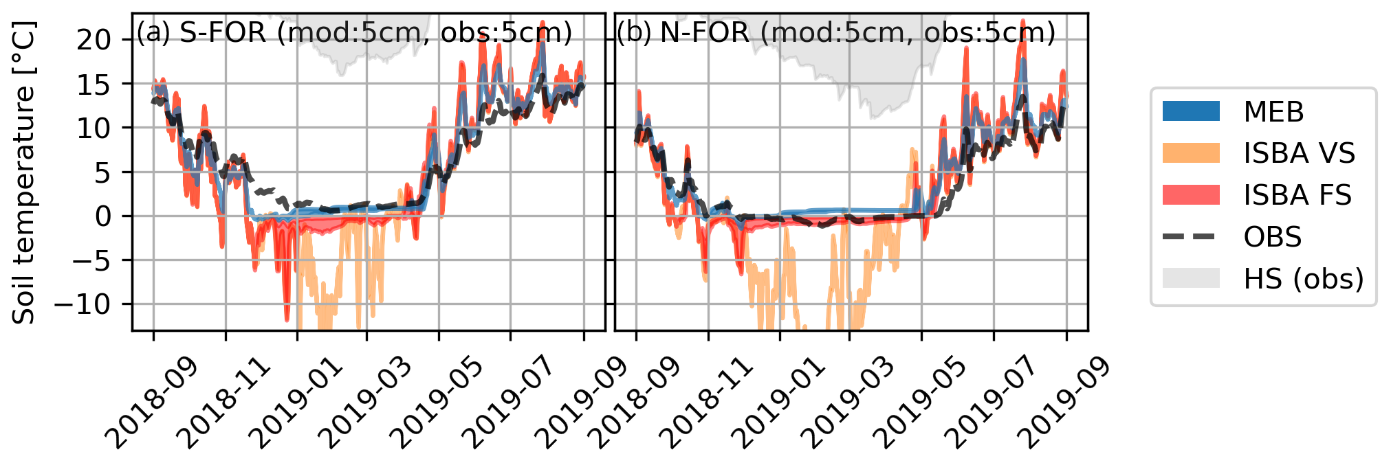
Figure 10 Effect of alternative configurations of ISBA and MEB on soil temperatures. The envelopes visualize the corresponding ensemble spreads. The observed evolution of the snow depth (HS) is not to scale. The observed soil temperatures are compared to the closest model layer; the depths of measurements and simulations are presented in each panel.

3.3.3 Impact of vegetation representation on surface energy fluxes

Figure 11 compares the deterministic simulations (Sect. 2.5) by MEB and ISBA-VS against observed above-canopy energy fluxes at N-FOR. The snow cover periods are defined according to agreement between MEB simulations and observations, and thus the ISBA-VS simulations are often snow-free as seen in Fig. 9.

MEB is superior to ISBA-VS in simulating energy fluxes. SWU simulations with snow cover are clearly improved by MEB, but the spread remains relatively large and albedo is underestimated when incoming radiation is small and overestimated when incoming shortwave radiation is higher. The time evolution of albedo on N-FOR and S-FOR is presented in Sect. 3.3.4. The LWU is very well simulated by both model configurations. Turbulent fluxes are clearly better simulated by MEB, but the performance metrics of turbulent fluxes are worse than for radiative fluxes. ISBA-VS uses the vegetation fraction parameter to scale the partitioning of latent heat flux between vegetation and soil (Eq. 4). However, because the same roughness length and thus turbulent exchange coefficient (C_H) is used for both soil and vegetation, the soil evaporation and snow sublimation are likely overestimated and result in clearly wrong partitioning between H and LE (Fig. 11c, d and g, h). In the case of N-FOR, especially the summer energy fluxes were majorly improved by simply assigning the vegetation fraction to unity (i.e., full vegetation coverage and no soil evaporation; see Fig. S7).

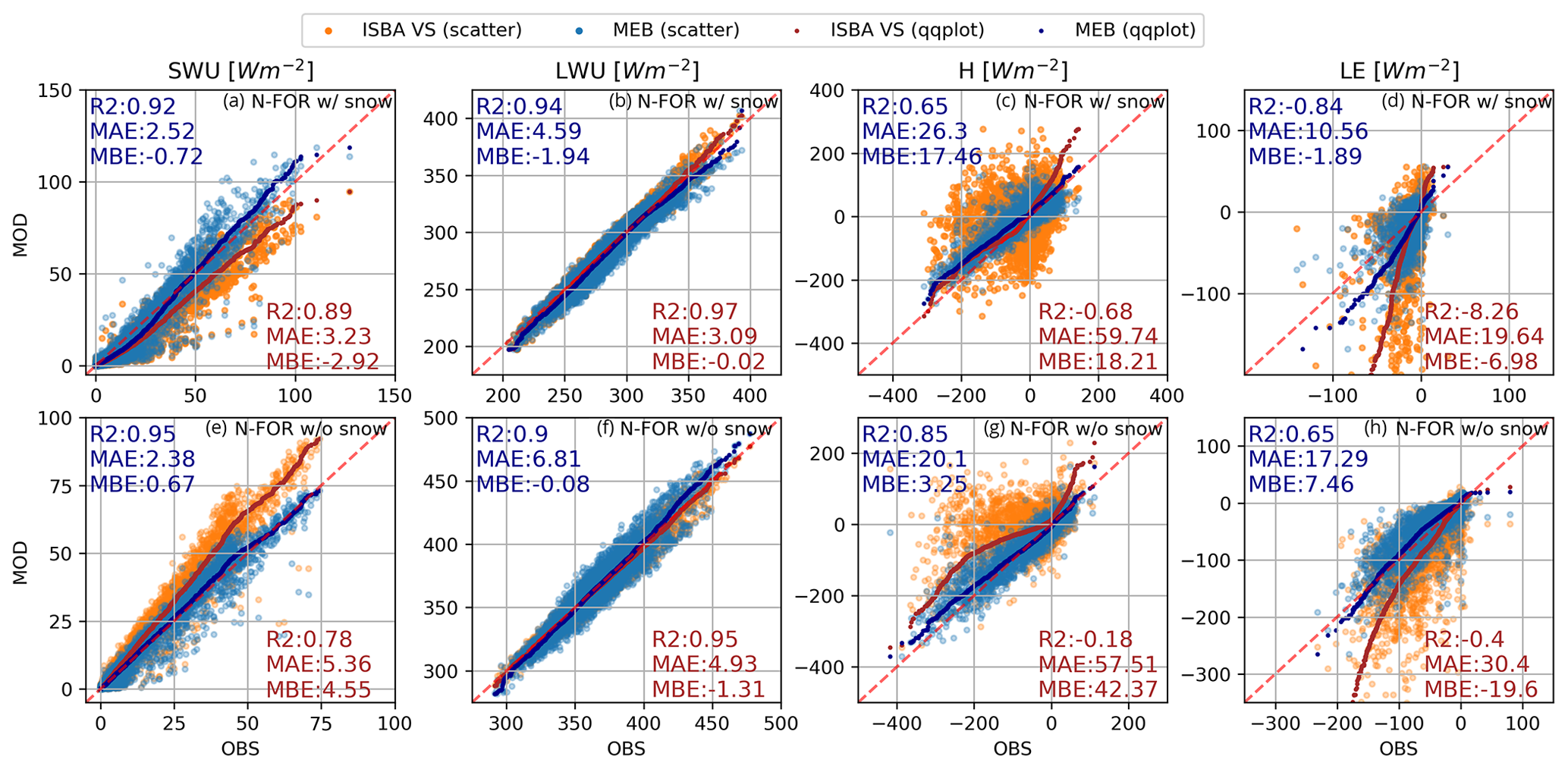
Figure 11 Simulated against observed upward shortwave and longwave radiation (SWU and LWU, columns 1 and 2) and turbulent fluxes (H and LE, columns 3 and 4) on the N-FOR site for the full evaluation period. Ground conditions are presented as (i) with snow cover (w/ snow, row 1) and (ii) without snow cover (w/o snow, row 2).

3.3.4 Evolution of albedo

Figure 12 illustrates the time evolution of modeled and observed albedo and the shortwave components in 2018–2019 on both forest sites. Compared to the measurements, the modeled early and midwinter albedos are underestimated, while the spring albedos are slightly overestimated, consistent with results in Sect. 3.3.3. The likely reason for winter albedo underestimation is because the models do not represent changes in albedo due to intercepted snow. The overestimation in spring is presumably due to representing the effective albedo of snow and forest canopy with only bulk canopy parameters, as well as effect of spring needle and litter fall decreasing snow albedo. Moreover, the simulated albedo is dominated by the vegetation albedo parameter, and thus it is not highly sensitive to snowpack albedo dynamics.

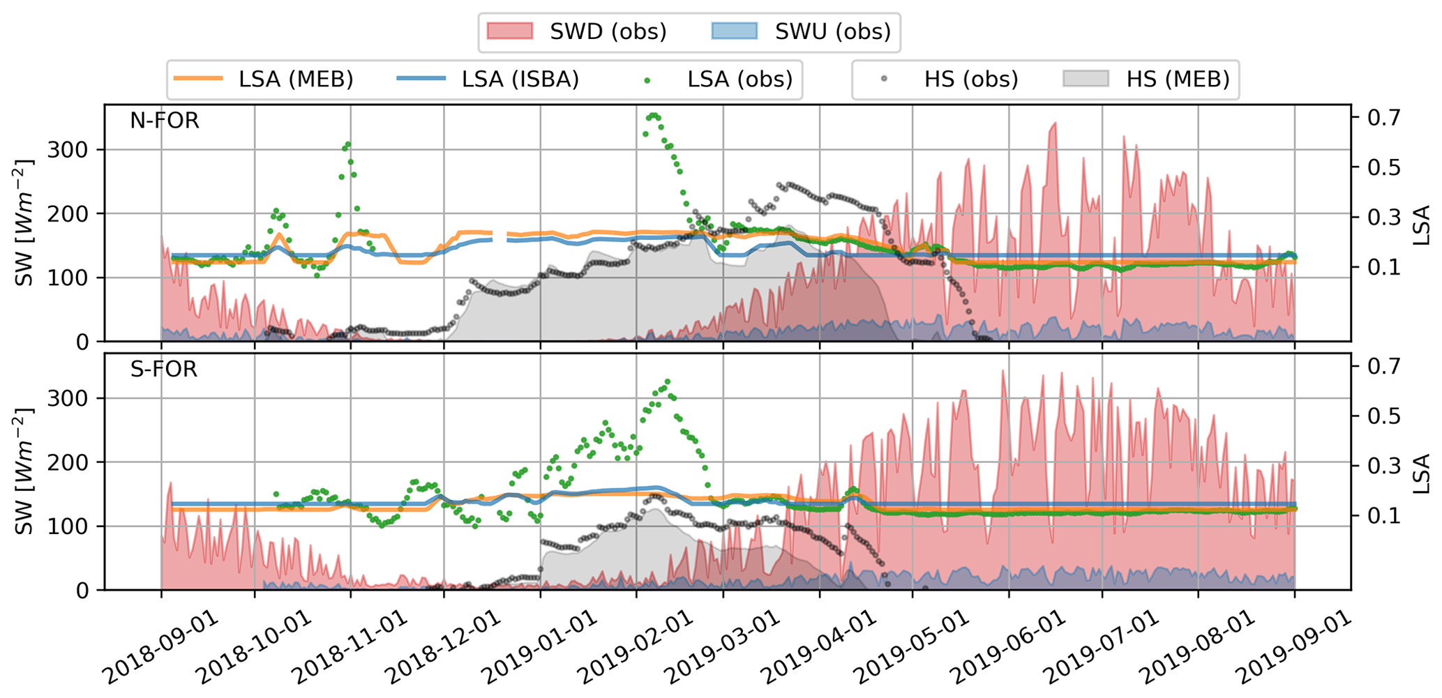
Figure 12 Simulated and observed albedo (LSA) and downward and upward shortwave radiation (SWD and SWU) in 2018–2019. LSA is presented as 5 d rolling means. The observed evolution of the snow depth (HS) is not to scale.

3.4 Summary: surface energy budget on peatland and forest sites

Finally, to sum up the whole surface energy budget, we compare how the simulated R_n and turbulent fluxes (H+ LE) match the observations at the four sites. These deterministic simulations are conducted with simulation setups that provided the best fit to data: the deterministic simulation as M98-SOC for the peatland sites and deterministic MEB simulation for the forest sites (Fig. 13).

Despite the challenges in simulating snow depth evolution at the forest sites, the energy budget simulations are generally better than on the peatlands. Due to the challenges to accurately simulate albedo and surface temperatures on the open sites, the simulated R_n is considerably worse on peatland sites than on forests (see Fig. 7). In particular, the high R_n periods, representing the spring conditions, are biased on peatland sites, while the negative R_n period (i.e., the winter conditions) are simulated rather well. The challenges in describing forest wintertime albedo and thus SWU (as in Figs. 12 and 11) do not significantly bias the R_n simulations, as in wintertime the shortwave radiation balance has a small role compared to the longwave radiation balance. The results propose that canopy temperature, which particularly in dense forests (e.g., S-FOR) has a central role for upward longwave radiation, must be adequately simulated by MEB. When it comes to the turbulent fluxes, the simulations capture the main seasonal patterns. However, there are still high uncertainties (scatter) both on peatland and forest sites. The relative uncertainties in simulated and observed energy fluxes are significantly greater in winter than in summer. Performance of the simulated summer energy fluxes is very good (Fig. S4).

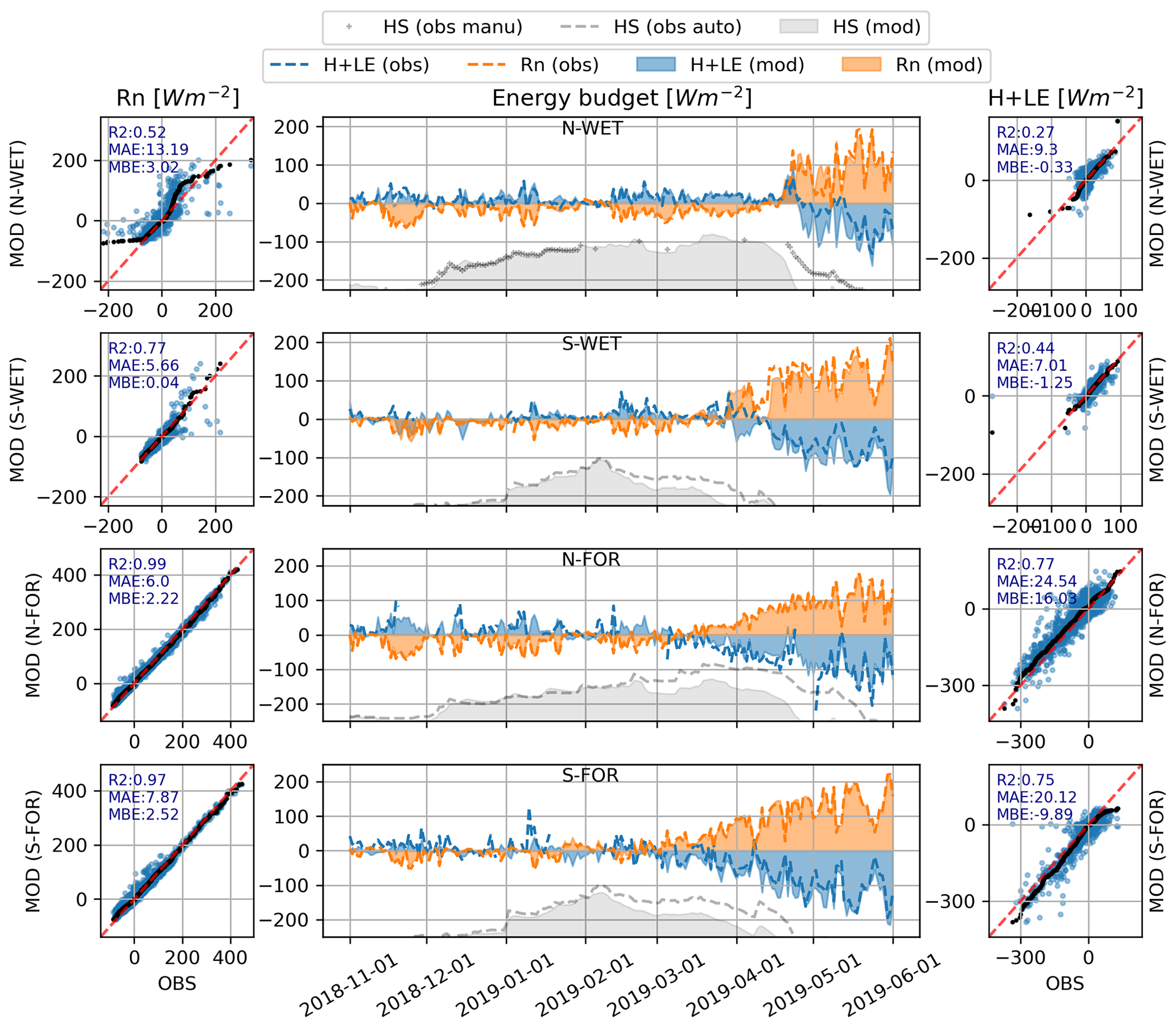
Figure 13 Simulated (MOD) against observed (OBS) daily surface energy budget during winter 2018–2019. The left column shows net radiation (R_n) and the right column presents the sum of turbulent fluxes (H+ LE). The scatterplots represent the full simulation periods when snow cover was present. The observed evolution of the snow depth (HS) is not to scale.

4 Discussion

4.1 Insights on energy flux partitioning in boreal environments

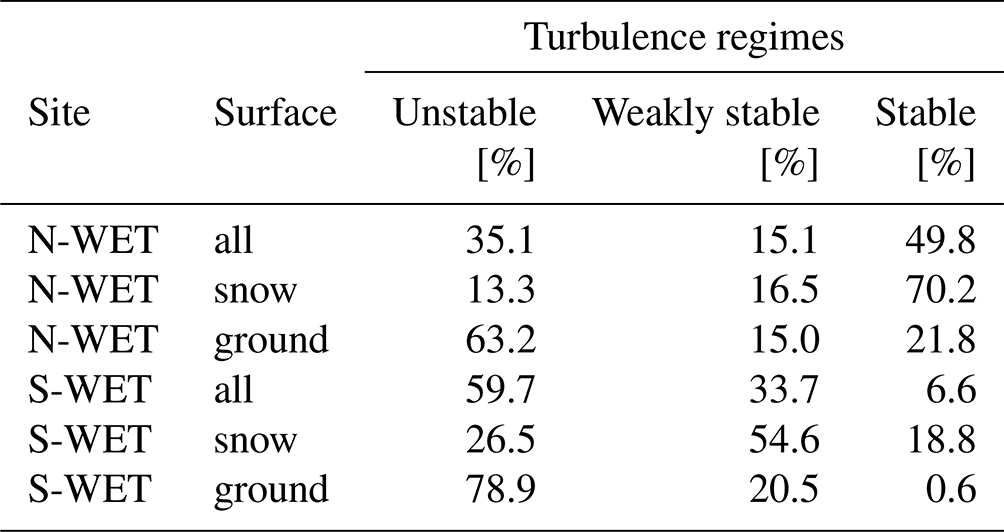
The energy budget observed with this novel dataset over boreal and subarctic peatlands showed that despite the prevailing stable atmospheric conditions (Table 3), the radiative cooling was mostly counterbalanced by sensible heat flux (H) (Fig. 3). During the snow season, the dominating regimes were strongly stable at N-WET (70.2 %) and weakly stable at S-WET (54.6 %). Despite the stronger stability at N-WET, we observed higher H fluxes compared to S-WET and considerably higher H than Lackner et al. (2022) at the Canadian site dominated by weakly stable conditions. Thus, we presume that greater radiative cooling leads to a stronger near-surface air temperature gradient and larger downward sensible heat flux.

The small role of the ground heat flux (G) at the studied peatlands is due to the high heat capacity of the peat soil and its large water storage which progressively freezes from the top, keeping the temperatures in the soil–snow interface nearly constant at a minimum of 0 ^∘C (Fig. 8). Other studies in tundra environments of the Canadian Arctic, Siberia and Svalbard have reported larger contributions of G to the wintertime energy budget (Lackner et al., 2022; Langer et al., 2011; Westermann et al., 2009).

Table 3 Occurrence of different turbulence regimes at S-WET and N-WET. The regimes are defined based on the bulk Richardson number (Ri): unstable conditions as Ri<0, weakly stable conditions as $\mathrm{0}\le Ri\le \mathrm{0.25}$ and strongly stable conditions as Ri>0.25.

We observed a shorter snowmelt period in the peatlands compared to adjacent forest sites (see Fig. S5), in line with Lundquist et al. (2013), who proposed that increased canopy shading (delaying melt) outweighs the impact of longwave radiation enhancement (accelerating melt). Our datasets support this (Fig. S5); however, the forest sites tended to also accumulate more snow than the peatland sites (wind erosion is presumably higher on peatlands), which may have contributed to longer snow duration in the forest.

4.2 Implications for simulating snow and energy balance at peatland sites

Our results highlighted the uncertainties in modeling turbulent fluxes over snowpack and identified the turbulent exchange parameterizations (M98-SOC and RI2-SOC) that improve the simulated surface energy fluxes and snowpack dynamics at high-latitude winter conditions (Figs. 5, 6). In stable (winter) conditions, the uncertainties in turbulent fluxes are in line with Menard et al. (2021), Conway et al. (2018), and Lapo et al. (2019) and larger than in unstable (summer) conditions (Fig. S4). Moreover, the turbulent fluxes of sensible and latent heat have greater uncertainty than the radiation balance components (Fig. 13). The ESCROC-E₂ simulations showed that the turbulent exchange parameterizations also have an impact on snowmelt simulations, in line with simulations at Col de Porte, France, and ESM-SnowMIP sites (Menard et al., 2021). In contrast, Lackner et al. (2022) found only small differences between the Crocus turbulence parameterizations in their study in the Canadian Arctic, most likely due to smaller sensible heat fluxes and less frequent strongly stable conditions.

Improved surface temperature simulations by the M98-SOC (absolute biases decreased by 0.3 ^∘C at S-WET and 0.4 ^∘C at N-WET compared to RIL-SOC) provide support to Martin and Lejeune (1998) and Gouttevin et al. (2023), who adjusted the turbulent fluxes under stable conditions to reproduce surface and air temperature observations. The default ISBA turbulent flux parameterization (RIL), although widely used, e.g., in numerical weather prediction and general circulation models (Mahfouf et al., 1995; Salas-Mélia et al., 2005; Voldoire et al., 2013, 2019), provided the poorest fit with the observed surface heat fluxes and produced a cold bias in snow surface temperature (−0.4 ^∘C at S-WET and −1.1 ^∘C at N-WET). This finding is consistent with ESM-SnowMIP (Menard et al., 2021), where the default configuration of Crocus had one of the lowest skills for surface temperature simulations (−2 ^∘C mean cold bias) among the compared snow models. Even with the M98-SOC simulation we found a rather low skill of turbulent flux simulations. To summarize, our findings highlight the limitations of the Monin–Obukhov similarity theory to simulate turbulent fluxes under stable atmospheric conditions and emphasize the need for further model developments with observations in various environments.

The soil temperature simulations confirmed that it is necessary to realistically describe the organic peat soil hydraulic and thermal properties (Menberu et al., 2021; Morris et al., 2022; Mustamo et al., 2019) to accurately simulate soil thermal regime and consequent freezing–thawing processes in peatlands (Fig. 8) (Dankers et al., 2011; Lawrence and Slater, 2008; Nicolsky et al., 2007). This is line with Decharme et al. (2016), who implemented SOC parameterization in ISBA and showed improved soil temperature simulations across northern Eurasia. The implementation of water table dynamics and lateral flow could further improve the soil temperature simulations on boreal and subarctic peatlands. The thermal state and ice/liquid water content also have major cascading effects on runoff generation during snowmelt (Ala-Aho et al., 2021). Moreover, the interactions between low vegetation and snow are likely improved by using explicit vegetation (MEB in SURFEX). However, as MEB has never been applied on snow-covered low vegetation, additional development and evaluation beyond the scope of this study would have been required.

4.3 Implications for simulations at forest sites

4.3.1 ISBA-VS

We found the ISBA-VS to be largely biased towards correctly simulated surface energy fluxes at the expense of poor soil temperature and snow depth simulations, as a major part of the composite was always directly coupled to the atmosphere (Figs. 9, 10). ISBA-VS with correct tuning (e.g., setting the veg fraction to unity on N-FOR) may be an imperfect but sufficient compromise to simulate snow-free forests in applications that first and foremost require grid-cell-averaged surface energy fluxes (i.e., numerical weather prediction). However, we agree with Napoly et al. (2020) that the snow cover fraction approach of ISBA (Fig. 2b) is essentially a compromise that attempts to retain the insulating impact of the snowpack over the soil while still simulating turbulent exchange from the vegetation. The energy exchange between the atmosphere and the soil–vegetation composite directly impacts the snowpack, and it led to strongly biased snow depth simulations, similar to Napoly et al. (2020). This fractional approach and high sensitivity of empirically based parameters (e.g., veg fraction) highlights the uncertainties of ISBA-VS to provide accurate year-round lower-boundary conditions of boreal forests for numerical weather prediction and general circulation model applications. Also considering the very low skill obtained in snow depth and soil temperatures for this configuration, its use in hydrological applications or surface offline reanalyses (Le Moigne et al., 2020) is highly questionable. Nevertheless, local-scale evaluation might not directly translate to large-scale spatial simulations, as further discussed in Sect. 4.4.

4.3.2 ISBA-FS

We found that snow and soil simulations in forests were strongly improved when the snow cover fraction was set to unity (ISBA-FS), allowing the snowpack to fully insulate the soil, similarly to the simulations at the peatland sites (Fig. 9). These results suggest that if the focus is on snowpack dynamics and soil temperature simulations, ignoring snow–vegetation interactions is a better compromise than using varying snow cover fraction as it is currently implemented in SURFEX. Consequently, ISBA-FS should be preferred to ISBA-VS in surface reanalyses as in Brun et al. (2013) and Vernay et al. (2022). However, ISBA-FS reaches its conceptual limits when forest energy balance, snow and soil state variables are all of interest. For instance, neglecting snow interception and subsequent canopy snow losses may cause large errors in simulated snow water equivalent in dense forests, and unrealistic contribution of the canopy evapotranspiration may be expected if reanalyses are further used for hydrological modeling. Obviously, highly biased surface energy fluxes would also be expected for any coupling with an atmospheric model.

4.3.3 MEB

MEB appears as a better compromise than ISBA-VS and ISBA-FS for modeling forest energy exchanges; the snow depth and soil temperature simulations were highly improved compared to ISBA-VS, while surface–atmosphere energy fluxes are obviously much more realistic than with ISBA-FS. Significant improvements in energy flux simulations were also obtained compared to ISBA-VS (Fig. 11).

Nevertheless, two systematic biases affecting upward shortwave radiation were identified: albedo was underestimated in winter and overestimated in spring (Fig. 12). The winter albedo underestimation was most likely because intercepted snow increased the observed albedo, a process that is not accounted for in MEB (Napoly et al., 2020). This assumption is based on Pomeroy and Dion (1996), while the increase in forest albedo by intercepted snow has been more recently shown (Webster and Jonas, 2018), and simple descriptions can already be found in some forest snow models (Mazzotti et al., 2020a). Although our results propose that the intercepted snow has a clear impact on the albedo, its impact on R_n was small. The spring albedo bias is in line with Malle et al. (2021), who found albedo at sparse boreal forests to be overestimated by the LSM CLM5. Big-leaf canopy parameterizations may fail to fully capture canopy shading, particularly at low solar elevation angles typical of high latitudes (Malle et al., 2021).

In contrast to Napoly et al. (2020), we found MEB to simulate snowmelt too early, especially on N-FOR (Fig. 9). These errors are partly explained by inaccuracies in canopy radiative transfer, but they also suggest errors in simulated below-canopy surface heat fluxes. The differences in snow simulations were rather small between MEB and ISBA-FS, especially at N-FOR, suggesting that sparse canopies did not majorly alter simulated snow accumulation and ablation, at least when compared to snow depth observations between the trees. Consistently, Meriö et al. (2023) have shown decreased snow depths at the immediate vicinity of tree trunks but high snow depth between trees at N-FOR.

4.4 Limitations and outlook

Our eddy-covariance fluxes are among the longest datasets ever used for the evaluation of turbulent flux simulations over snow. The EC data, however, contain both random and systematic uncertainties (e.g., Aubinet et al., 2012). The absolute values of winter H and LE are small, and their relative uncertainty is high; compared to summertime measurements, the wintertime energy balance closure ratio is typically poorer, particularly at the northern ecosystems (Reba et al., 2009; Molotch et al., 2009; Launiainen, 2010). As our analysis used numerous site years from multiple sites, and we used established quality criteria for filtering the EC fluxes, we expect that uncertainties in flux data do not significantly affect the study results. Moreover, the conclusions regarding the validity of each model version were not affected by the selected flux quality flag (Sect. 2.4.2). Intrinsic uncertainties in meteorological forcing are known to exist, especially in northern conditions (instrument freezing, snow blocking, undercatch, etc., Stuefer et al., 2020), and data gaps further add up possible sources of errors. Uncertainties in model forcing can affect model–data comparisons, especially during the gap-filled periods (Raleigh et al., 2015).

Potentially important snow processes on subarctic sites are still absent in Crocus, including wind-induced snow transport and internal water vapor transfer due to a large temperature gradient in the snowpack. Wind can move and change the properties of snow (Pomeroy and Essery, 1999; Meriö et al., 2023; Liston and Sturm, 2002) and is especially noticeable on open peatlands. In Crocus, wind modifies the properties of falling snow (Vionnet et al., 2012) but without any lateral transport or modifications of the mass. Although we achieved satisfactory model performance without accounting for this process, Meriö et al. (2023) showed notable wind transport in transition zones between open peatland and forest at the N-WET site. Although the spatial scale of wind transport prevents an explicit simulation of this process in large-scale LSMs, improved parameterizations of the wind impact on snow properties should be considered in the future. Omission of internal water vapor transfer by diffusion and/or convection has been suspected to be responsible for errors in simulated snow properties (density, microstructure) in Arctic snowpack (Barrere et al., 2017; Domine et al., 2018) and consequently in thermal conductivity and soil thermal regime. A realistic implementation of water vapor transfer within the snowpack is lacking in most state-of-the-art LSMs. Complementary observations and model developments are required to understand if the simulated snow properties are affected by this kind of error. Furthermore, the spring and autumn conditions on the peatlands are particularly difficult to correctly simulate; in addition to the snow cover, also, e.g., ponding of liquid water and refreezing of the ponds are not uncommon (Noor et al., 2022) and can alter the albedo.

In forests, the spatial heterogeneity of snow cover can be high, as demonstrated by numerous studies (Marttila et al., 2021; Mazzotti et al., 2020b; Noor et al., 2022) and confirmed by our data (Fig. 9). The small-scale forest structure has an important role in the evolution of the snow cover and may affect the representativeness of point measurements (Bouchard et al., 2022). Consequently, the comparison of point observations and models intended for forest stand and larger scales (such as the big-leaf approach of MEB) can suffer from this scale mismatch (Essery et al., 2009; Rutter et al., 2009). More realistic below- and above-canopy heat flux simulations could be achieved by more sophisticated canopy representations, including multiple layers and species (Bonan et al., 2021; McGowan et al., 2017; Launiainen et al., 2015; Gouttevin et al., 2015). For site-level or limited-area modeling, high-resolution models that explicitly resolve tree-scale canopy structure are a promising alternative to traditional LSMs (Broxton et al., 2015; Mazzotti et al., 2020b).

The generality of our findings should be tested by additional snow model and LSM evaluation studies, extended to more contrasting climates and a wider range of ecosystem types. For this purpose, model evaluation datasets should be complemented with more boreal and Arctic sites and observations of all components of surface energy balance, particularly turbulent fluxes.

5 Conclusions

We used eddy-covariance-based energy flux data, radiation balance, and snow depth and soil temperature measurements in two boreal and subarctic peatlands and forests to evaluate turbulent exchange parameterizations and alternative approaches to represent the soil and vegetation continuum in land surface models. We used the SURFEX platform, but our findings are largely transferable to other model systems. Our evaluation with the ensemble snowpack parameterizations (ESCROC-E₂) ensures that uncertainties in snow processes (not evaluated in this study) do not affect the robustness of our main conclusions.

Peatland simulations showed that using a stability correction function that increases the turbulent exchange under stable atmospheric conditions is imperative to simulate the snowpack energy budget. This adjustment led to major improvements under stable conditions during snow cover, but the model performance still remained lower than in snow-free conditions. Furthermore, correct hydraulic and thermal parameterization of organic peat soils was found necessary to reproduce the observed soil thermal regime in peatlands. The findings have direct implications for modeling snow dynamics, peatland hydrology and permafrost dynamics.

The surface energy budgets of forest sites were well simulated by the explicit big-leaf approach (MEB), while the composite soil–vegetation approach (ISBA-VS) performance was satisfactory only after an adjustment of a sensitive vegetation fraction parameter. In particular, shortwave and longwave radiation balances were simulated well by both approaches, whereas the turbulent fluxes had significantly higher uncertainty. Only the explicit vegetation model (MEB) was able to simultaneously simulate realistic surface energy budget, snow and soil conditions. The composite approaches only succeeded in simulating either the correct surface energy budget (ISBA-VS) or snow and soil conditions (ISBA-FS). Furthermore, we demonstrated that the composite approaches rely on a previously poorly documented parameterization of the snow cover fraction with high sensitivity on model outputs despite a limited physical interpretation.

With well-selected model configuration and parameterization, the SURFEX model platform can realistically simulate surface energy fluxes and snow and soil conditions in the subarctic and boreal peatlands and forests. The common version of ISBA (ISBA-VS) can provide rather realistic lower-boundary conditions for numerical weather prediction and global circulation models, at the expense of non-realistic predictions of forest snow and soil conditions necessary for hydrological applications. We expect that the future inclusion of MEB in operational systems will reconcile these applications. Our results can be used to inform the choice of model configuration for studies of subarctic and boreal region ecology, hydrology and biogeochemistry under the ongoing environmental change.

Appendix A: Tables of abbreviations, acronyms and mathematical symbols

A1 Table of acronyms and abbreviations

Acronyms and abbreviations	Definition
LSM	Land surface model
LSA	Land surface albedo
LAI	Leaf area index
LWD	Downward longwave radiation
LWU	Upward longwave radiation
SWD	Downward shortwave radiation
SWU	Upward shortwave radiation
H	Sensible heat
LE	Latent heat
Rn	Net radiation
G	Snowpack–ground heat flux
SOC	Soil organic content
EC	Eddy covariance
HS	Snow depth
RIL	Classical Louis (1979) formula for the turbulent exchange coefficient
RI1	RIL with threshold at Ri=0.1
RI2	RIL with threshold at Ri=0.026
M98	Martin and Lejeune (1998) formula for CH
BOGR	Boreal grass
BONE	Boreal needleleaf evergreen
FMI	Finnish Meteorological Institute
SMEAR	Station for Measuring Forest Ecosystem–Atmosphere Relations
FST	Flux stationarity

A2 Table of mathematical symbols

Symbol	Definition
ϵ	surface emissivity
σ	Stefan–Boltzmann constant
Ts	surface temperature
ρa	air density
ρw	liquid water density
ρ	snow density
cp	specific heat capacity
Va	wind speed
Ta	air temperature
CH	turbulent exchange coefficient
ET	total evapotranspiration
Eg	evaporation from the bare soil surface
Ec	evaporation of intercepted water on the canopy
Etr	transpiration from the vegetation
Si	sublimation from bare soil ice
Lv	latent heat of vaporization
Lf	latent heat of fusion
veg	fraction of vegetation cover
qsat(Ts)	saturated specific humidity at the surface
qa(Ts)	atmospheric specific humidity
hu	dimensionless relative humidity at the ground surface related to the superficial soil moisture content
hv	dimensionless Halstead coefficient describing the Ec and Etr partitioning
	between the leaves covered and not covered by intercepted water
zu	reference height of the wind speed
za	reference height of the air temperature and humidity
z0t	roughness height for heat
k	von Kármán constant
Ri	bulk Richardson number
Cv	effective heat capacity of the canopy
Cg,1	effective heat capacity of the ground surface/litter layer (uppermost layer)
Cn,1	effective heat capacity of the snowpack (uppermost layer)
Tv	temperature of the canopy
Tg,1	temperature of the ground surface/litter layer (uppermost layer)
Tn,1	temperature of the snowpack (uppermost layer)
Rnv	net radiation of the canopy
Rng	net radiation of the ground surface/litter layer
Rnn	net radiation of the snowpack
k	snow effective thermal conductivity
LEs	latent heat flux of the snowpack
Gn	heat conduction at the snow–soil interface
psn	effective snow cover fraction
psnv	effective snow cover fraction of the vegetation
psng	effective snow cover fraction of the soil
HSg	threshold value for height of the snow
wsw	coefficient relating to vegetation characteristics
E2	ESCROC optimized standard subensemble
P	precipitation rate
Pice	snowfall rate
Pliq	rainfall rate
r	diffuse-to-total-shortwave-radiation ratio
μ	cosine of the sun zenith angle
u*	friction velocity

Appendix B: Model evaluation data availability and radiation forcing evaluation

The availability periods of the model evaluation data are presented in Table B1.

Table B1 Model evaluation data availability for each site.

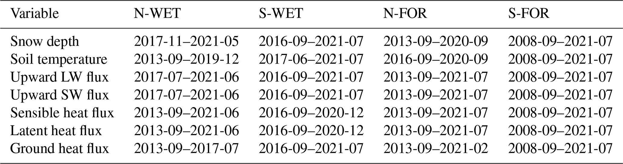
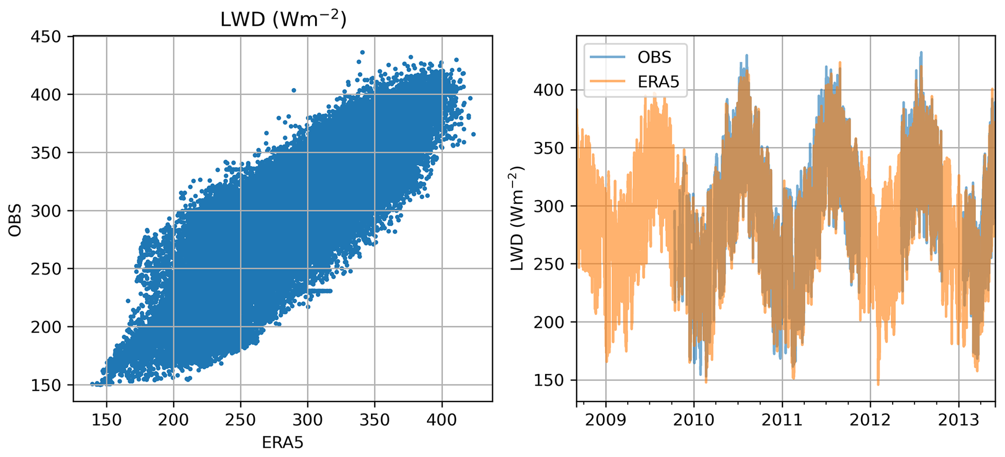
Figure B1 Comparison of longwave radiation forcing data between ERA5 and site observations (OBS) on S-FOR.

Appendix C: Effect of snow cover fraction parameter w_sw

Bengtsson et al. (2017)Courtier et al. (1991)Decharme et al. (2019)Caillaud et al. (2021)Nabat et al. (2020)Le Moigne et al. (2020)Verrelle et al. (2021)Vernay et al. (2022)Brun et al. (2013)Morin et al. (2020)

Table C1 Summary of snow cover fraction and values of w_sw used in different SURFEX/ISBA applications. The parameter w_sw is rarely documented, and hence these application-specific values were obtained through communications with the authors.

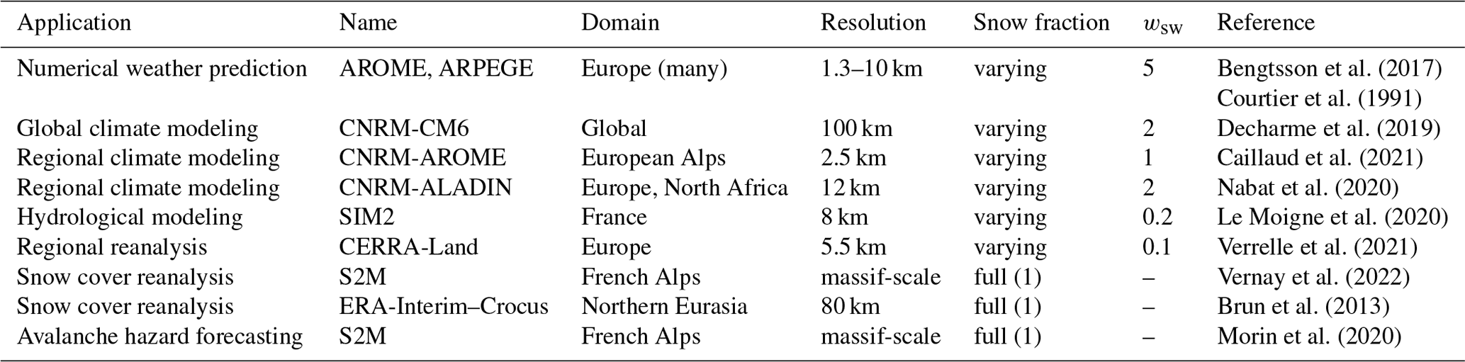
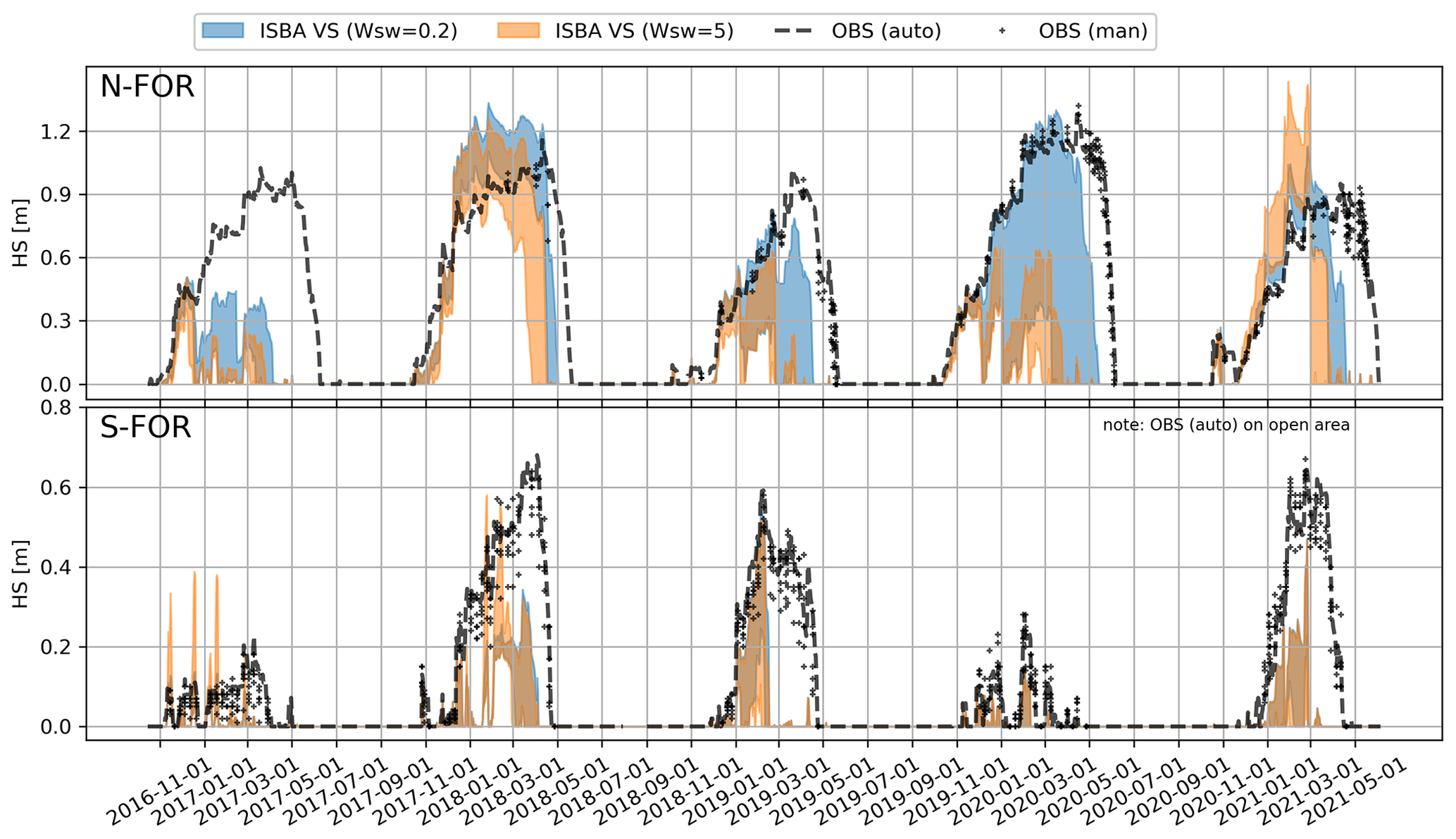
Figure C1 Effect of w_sw parameter on snow depths simulated by ISBA-VS. The envelopes visualize the corresponding ensemble spreads between minimum and maximum values.

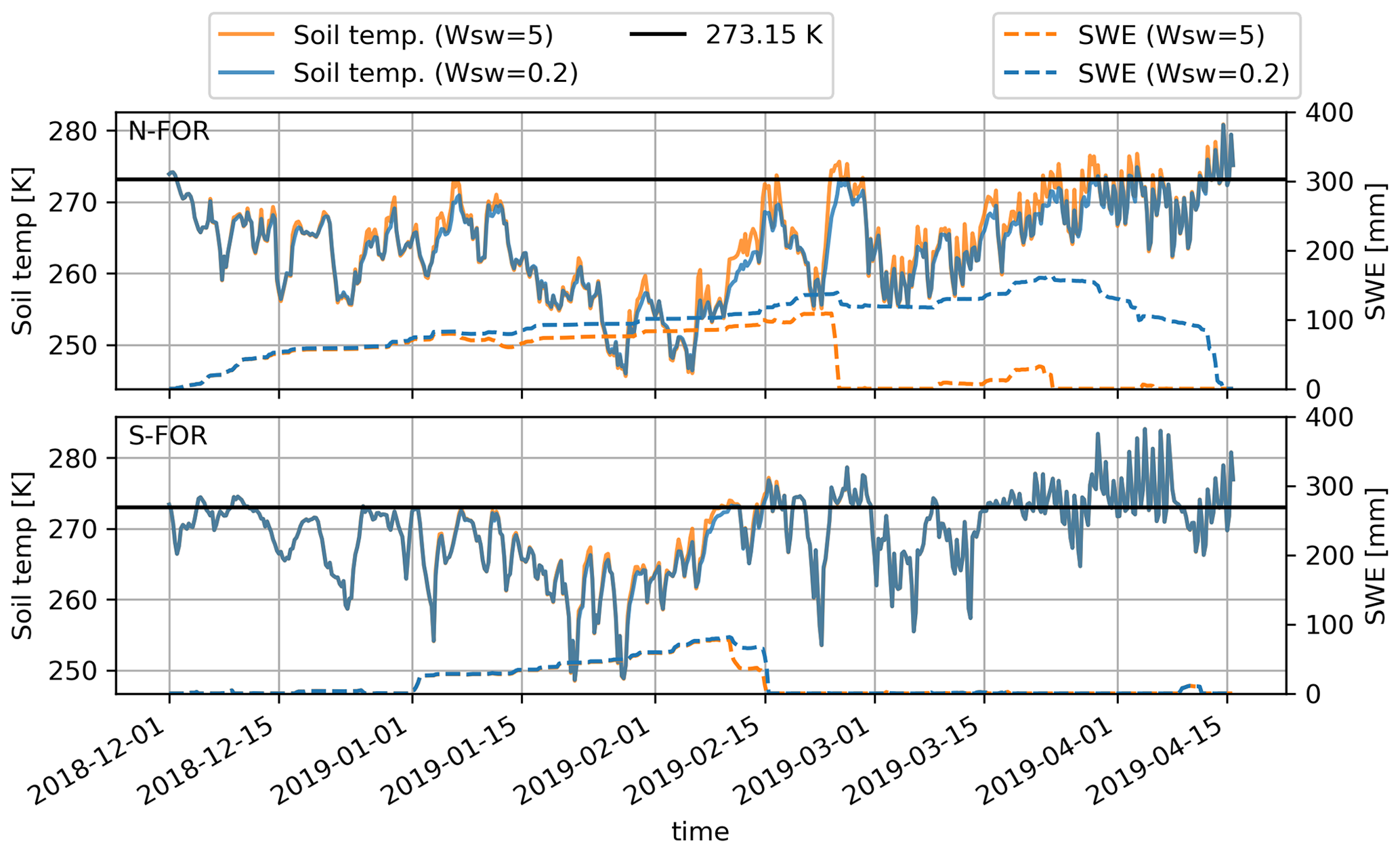
Figure C2 The sensitivity of the w_sw parameter on 6 h surface soil temperature simulations and snow water equivalent (SWE). Simulations are represented by one member of the ESCROC-E₂ ISBA-VS.