the Creative Commons Attribution 4.0 License.
the Creative Commons Attribution 4.0 License.
 | 23 Apr 2024
A 3D glacier dynamics–line plume model to estimate the frontal ablation of Hansbreen, Svalbard
José M. Muñoz-Hermosilla
Jaime Otero
Eva De Andrés
Kaian Shahateet
Francisco Navarro
Iván Pérez-Doña
Frontal ablation is responsible for a large fraction of the mass loss from tidewater glaciers. The main contributors to frontal ablation are iceberg calving and submarine melting, with calving often being the largest. However, submarine melting, in addition to its direct contribution to mass loss, also promotes calving through the changes induced in the stress field at the glacier terminus, so both processes should be jointly analysed. Among the factors influencing submarine melting, the formation of a buoyant plume due to the emergence of fresh subglacial water at the glacier grounding line plays a key role. In this study we used Elmer/Ice to develop a 3D glacier dynamics model including calving and subglacial hydrology coupled with a line plume model to calculate the calving front position at every time step. We applied this model to the Hansbreen–Hansbukta glacier–fjord system in southern Spitsbergen, Svalbard, where a large set of data are available for both the glacier and the fjord from September 2008 to March 2011. We found that our 3D model reproduced the expected seasonal cycle of advance–retreat. Besides, the modelled front positions were in good agreement with the observed front positions at the central part of the calving front, with longitudinal differences, on average, below 15 m for the period from December 2009 to March 2011. But there were regions of the front, especially the eastern margin, that presented major differences.
- Article
(5873 KB) - Full-text XML
- BibTeX
- EndNote


Svalbard is an Arctic region with a very high climatic sensitivity (Isaksen et al., 2016; Nordli et al., 2020). The ongoing climate change context affects the dynamics and mass balance of glaciers, as well as the ocean’s thermal and dynamical processes. This leads to hydrological and ecological effects at regional and global scales, including sea level rise. Although the global glacier volume is only a small fraction of that of the Antarctic and Greenland ice sheets, glaciers are currently losing more mass than both sheets taken separately and are doing so at similar or larger acceleration rates (Hugonnet et al., 2021). In fact, according to the Sixth Assessment Report of the IPCC of 2021 (Masson-Delmotte et al., 2021), glaciers' contribution to sea level rise has been very significant for the period from 1971 to 2018 (22 % of the total estimation). The main reason for this is the high sensitivity of glaciers to atmospheric and oceanic forcing (Rignot et al., 2010; Motyka et al., 2013; Straneo and Cenedese, 2015; Luckman et al., 2015; Holmes et al., 2019). The mass change rate of Arctic glaciers, including Greenland's periphery, during the period from 2000 to 2018 reached −124.6 Gt a−1 and represents 46.7 % of the total rate for all the glaciers around the world (Hugonnet et al., 2021). Frontal ablation of tidewater glaciers (mainly calving and submarine melting) represents between 10 % and 30 % of this loss in regions such as Svalbard and the Russian Arctic (Huss and Hock, 2015; Hanna et al., 2020). Actually, among the seven northern glacierized regions studied by Kochtitzky et al. (2022), the Russian Arctic experienced the highest frontal ablation rate during the period 2000–2020, followed by Svalbard.
The entire volume of water stored in Arctic glaciers, if melted completely, could raise the sea level by around 0.3 m (AMAP, 2017). The projections for this region through the 21st century show that its contribution will be significant (Meier et al., 2007; Church et al., 2013; Hock et al., 2019), so, by the end of this period, the estimated ice loss from Arctic glaciers is expected to contribute between 3.9 and 9.2 cm to sea level rise, around 56 % of the global glacier estimation (Edwards et al., 2021). In the case of Svalbard, the contribution to sea level rise is estimated at between 0.75 and 1.25 cm (Edwards et al., 2021).
Tidewater glaciers are glaciers that terminate in the sea, with their terminus either floating or grounded below the sea level (Cogley et al., 2011). The terminus position of these glaciers is an essential climate variable that helps us to understand important processes such as glacier mass balance or ice–ocean interactions (Bojinski et al., 2014). There have been many studies on the evolution of the front position of tidewater glaciers based on remote sensing data (e.g. at the local level; Błaszczyk et al., 2021), but the relative importance of the various processes driving the front position changes remains poorly understood due to the scarcity of in situ measurements. This scarcity is extreme in the case of basal conditions and subglacial hydrology. Besides, the zone close to the calving front is most often heavily crevassed, preventing measurements that could be useful for constraining processes such as calving and submarine melting. Some recent works have started to cover this scarcity of direct measures with observations and the use of models regarding fjord water properties (Jackson et al., 2017, 2019), glacier front alterations (Vallot et al., 2019) or the whole glacier–fjord scheme (Cassotto et al., 2018; Jouvet et al., 2018; Sutherland et al., 2019; Xie et al., 2019). However, current understanding relies heavily on parameterizations of melting and entrainment, for which there is little in the way of validation (Hewitt, 2020). Summarizing, many features of tidewater glaciers still remain under-observed and poorly characterized.
Computational models can help in understanding processes and predicting the future evolution of glaciers, yet they require at least a minimum of observational input data. Moreover, the more realistic and complex models require a larger variety and number of input data. In terms of calving, for example, the development of a simple calving law is still an unsolved problem (Benn et al., 2017; Benn and Åström, 2018). Therefore, the use of computationally expensive 3D calving models to reproduce the process with a fair degree of agreement with reality becomes necessary (Todd et al., 2018, 2019). In terms of submarine melting at tidewater glaciers, Jenkins (2011) implemented a one-dimensional plume model by adapting his previous work (Jenkins, 1991) based on the theory of Morton et al. (1956), finding a relation between the subglacial runoff and the submarine melt rate. This model has been used to compute submarine melting in tidewater glaciers (Cownton et al., 2015, 2019; Slater et al., 2015, 2018). Cook et al. (2020, 2022) studied both calving and subglacial melting by coupling subglacial hydrology and meltwater plumes to a 3D glacier dynamics model. These authors found significant results concerning the subglacial hydrology and its relationship with calving and plume processes, but they did not focus their work on the glacier terminus evolution. The front evolution, though, has been studied by some authors (Otero et al., 2017; De Andrés et al., 2018) using 2D models, evidencing the role of back pressure and the importance of oceanic and atmospheric processes. Even so, the lack of the third dimension in the latter models has prevented incorporating important dynamical 3D effects, such as lateral front melting. The two last-mentioned models were applied to the Hansbreen–Hansbukta glacier–fjord system, Svalbard, which is our focus of interest, but these are not the only modelling works that refer to this system. Oerlemans et al. (2011) proposed a minimal glacier model in which the ice mechanics is strongly parameterized. The simple law for iceberg calving used in their model was able to match observed and simulated glacier length since 1900. Vieli et al. (2000, 2002) found that basal-sliding processes strongly depend on the effective pressure and control the flow and the retreat of Hansbreen. Pętlicki et al. (2015), on the other hand, concluded that calving on Hansbreen is mainly triggered by the local imbalance of forces at the front due to undercutting at the sea waterline and development of a thermo-erosional notch. More recently, De Andrés et al. (2021) made a comparison between a 2D glacier–fjord model and a 2D glacier–plume model regarding the calving front evolution. They determined that both models showed similar results for simulated glacier front positions under appropriate constraints of subglacial discharge, fjord temperature and crevasse water depth, but the glacier–plume model computational cost was significantly lower. Finally, Möller et al. (2023) presented a sensitivity study analysing the impact of five different bedrock datasets on projected mass losses from Hansbreen and suggested that under the influences of warmer climates, accurate bedrock/ice thickness data are especially important for future glacier evolution modelling on decadal timescales.
In this work we aim to fill some of the above gaps by presenting a 3D full-Stokes Elmer/Ice-based ice flow model focused on Hansbreen front evolution. To do so, we include atmospheric (through surface mass balance and surface meltwater), hydrological and oceanic processes (line plume model), and a 3D calving law. We run the model for a total of 30 months, from September 2008 to March 2011, and analyse the model performance by comparing the monthly front positions obtained with observational data. By including all elements involved in frontal ablation, this model is expected to be a valuable instrument to study the terminus evolution.
2.1 Study area
The glacier–fjord system Hansbreen–Hansbukta is located in one of the branches of the Hornsund fjord in southwest Spitsbergen, Svalbard, at ∼ 77° N, ∼ 15.6° E (Fig. 1). Hansbreen is a polythermal tidewater glacier flowing southward that covers an area of ∼ 57 km2. It is about 16 km long with a low mean surface slope of around 1.8° on average along the central flow line (Grabiec et al., 2012). Its calving front is 1.5 km wide with a vertical face ∼ 100 m thick at the central flow line, of which 50 to 60 m is below the sea level. The seasonal retreat of Hansbreen usually starts in June/July and lasts until late autumn/early winter, and the average summer and winter fluctuations amount to −125 and 79 m, respectively (Błaszczyk et al., 2021). As for Hansbukta, it is a ∼ 2 km long bay, with a maximum depth of ∼ 77 m. Temperature and salinity in Hansbukta experience strong seasonal variability, ranging from −1.8 to 3 °C and from 34.6 to 31.8 PSU between April and August, respectively.
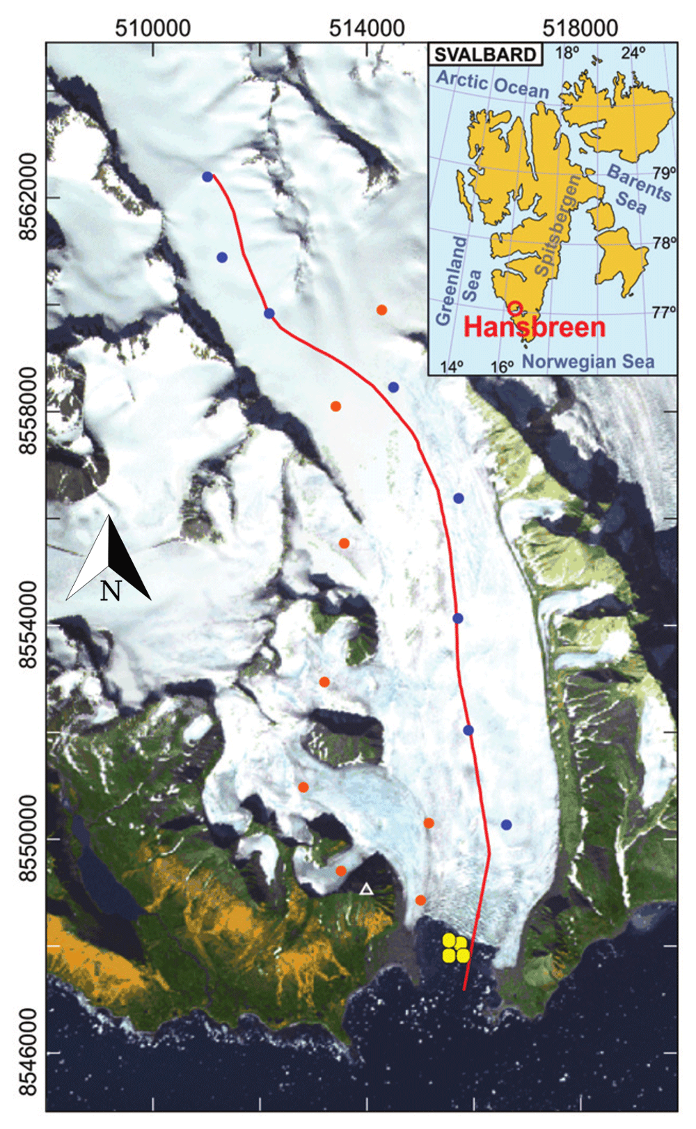
Figure 1Location of Hansbreen–Hansbukta, Svalbard (inset). ASTER image of Hansbreen–Hansbukta showing the location of the stakes for velocity measurements (blue circles for the flow line and red circles for the rest of the stakes) and the conductivity–temperature–depth (CTD) profiles in Hansbukta (yellow circles) (De Andrés et al., 2021). The white triangle indicates the position of the time-lapse camera. The axes include the UTM coordinates (m) for zone 33X.
Data
The model uses gridded surface velocity data as input. The ice surface velocities were obtained by applying Bayesian kriging (BK) techniques (Perez-Doña and Otero, 2023) (Fig. 2) to daily horizontal velocities measured between May 2005 and April 2011 at a set of stakes located along the glacier. As a prior for the BK, a distribution of the surface velocity module of Hansbreen was calculated as the averaged velocities derived from measurements taken by TerraSAR-X from January 2013 to August 2014 using feature tracking (Adrian Luckman, personal communication, 2014).
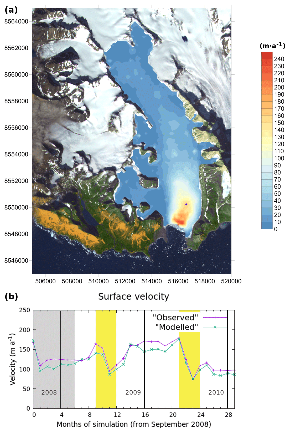
Figure 2(a) Hansbreen surface velocity distribution obtained from the BK algorithm corresponding to September 2008 and (b) time evolution of the velocity at the stake located closer to the calving front (the southernmost blue point in Fig. 1). The shaded area corresponds to the initialization period. The yellow areas indicate the summer periods, and the vertical black lines separate the different years. The satellite image used as background in (a) was available from ASTER © METI and NASA, all rights reserved, courtesy of the University of Silesia, Poland, within the frame of cooperation of the SvalGlac project.
Front position data from time-lapse camera images taken every 3 h were processed and averaged over weekly intervals between December 2009 and September 2011 (Otero et al., 2017). Surface mass balance (SMB) and surface meltwater (SMW) were obtained from downscaled European Arctic Reanalysis data at 2 km horizontal and hourly temporal resolutions, constrained by automatic weather stations and stake observations (Finkelnburg, 2013). The surface elevation came from the SPIRIT digital elevation model for gentle slopes, with a 30 m rms absolute horizontal precision and 40 m resolution. Bedrock topography was inferred from ground-penetrating radar data (Grabiec et al., 2012; Navarro et al., 2014).
Hydrographic data consist of a set of CTD casts (i.e. conductivity, temperature and depth profiles) in Hansbukta (yellow points in Fig. 1). All the data were vertically averaged every 1 dbar (1 kPa). Available CTD oceanographic data only covered the period from April 2010 to August 2010, with a long gap between April and July. Linear interpolation was used to fill in the period from April 2010 to July 2010. Since mooring data indicate that the temperature and salinity records remained relatively stable between November and April (De Andrés et al., 2018, their “Supplementary material”), a linear extrapolation was used to estimate temperature and salinity from August to November. The values for November (winter conditions) were extended until March.
2.2 Model
We use the open-source, full-Stokes, finite-element, ice flow model Elmer/Ice (Gagliardini et al., 2013) including the GlaDS (Glacier Drainage System) hydrological model (Werder et al., 2013), the free-surface evolution, a 3D calving module (Todd et al., 2018) and a continuous sheet-style “line” plume across the width of the calving front (Cook et al., 2020) to study Hansbreen front evolution from September 2008 to March 2011. We follow the work of Cook et al. (2022) but with an asynchronous coupling between the subglacial hydrology and the ice flow (and the calving and the plume); i.e. the subglacial hydrology that generates the plume is computed monthly, whereas the time step of the ice flow simulation is 1 d.
2.2.1 Ice flow model
The horizontal mesh is composed of triangles, and it has been designed to have a maximum resolution of 50 m at the calving front. The resolution decreases progressively upglacier, reaching 200 m at 5 km from the front. Beyond that, the mesh continues coarsening to get to 500 m at the head of the glacier. This horizontal mesh is then vertically extruded on 10 levels, resulting in a 3D mesh composed of triangular prisms. The model solves the full-Stokes equations for ice flow, with rheology defined by Glen's flow law (e.g. Cuffey and Paterson, 2010), and uses the calving implementation described by Todd et al. (2018, 2019) and Cook et al. (2020, 2022), following Otero et al. (2010) and Todd and Christoffersen (2014). This implementation is an improved formulation of the crevasse depth (CD) calving criterion postulated by Benn et al. (2007) and Nick et al. (2010) for use in a 3D framework. This calving criterion has been chosen because it is the one implemented in Elmer/Ice, but, when compared with other calving models such as the height-above-flotation model (HAF; Van der Veen, 1996), the fraction-above-flotation model (FAF; Vieli et al., 2001), the eigencalving model (EC; Levermann et al., 2012), the von Mises criterion (VM; Morlighem et al., 2016) and a calving relation based upon the surface stress maximum (SM; Mercenier et al., 2018), the results indicate that the crevasse depth calving model provides the best balance of high accuracy and low sensitivity to imperfect parameter calibration (Amaral et al., 2020). Moreover, a recent study of Benn et al. (2023) shows that the CD calving law reflects the glaciological controls on calving at a tidewater glacier (Sermeq Kujalleq) and exhibits considerable skill in simulating its mean position and seasonal fluctuations. Crevasse depths are, therefore, calculated following
where σn is the net stress (positive for extension and negative for compression). The terms on the right-hand side represent the balance of forces: the first corresponds to the opening force of longitudinal stretching, where τe represents the effective stress, and the sign function ensures that crevasses opening is only produced under longitudinal extension; the second term corresponds to the ice overburden pressure, which leads to creep closure, where ρi is the ice density, g is the acceleration of gravity and d stands for the crevasses' depth. Pw stands for the water pressure which contributes to opening the crevasses. This term is here considered to be zero for surface crevasses because they are capable of opening without water pressure. For basal crevasses, on the other hand, water pressure is controlled by the subglacial hydrological system and at the calving front can be expressed as
with ρw being the density of water at the calving front and Z the elevation with respect to sea level. Zsl denotes the sea level and is set to 0 m. This improved criterion specifies calving to occur either when surface crevasses reach the waterline or when surface and basal crevasses meet, and its formulation disregards the formation of new fractures. Such a simplification is justifiable given the extensively fractured nature of ice near the calving front; leading extensional stresses primarily serve to propagate existing fractures. To determine crevasse propagation, the calving model uses a separated 2D mesh representing the frontal area of the glacier. This mesh extends 1850 m up the glacier and has a resolution of 30 m. When calving occurs, the model calculates a calving vector which is normal to the calving front and maps pre-calving to post-calving node positions. In order to maintain the mesh quality, calving events require subsequent remeshing of the main mesh.
2.2.2 Boundary conditions
The calving front is determined by a series of nodes between two fixed points in the lateral margins of the glacier. Consequently, these nodes will be the ones that are allowed to advance and retreat. At the head of the glacier, the ice divide, horizontal velocities and shear stresses are set to zero. No flow is allowed through the lateral margins of the glacier, where no-slip conditions are additionally imposed. The upper free surface is constrained to a surface mass balance accumulation flux boundary condition (positive for accumulation, negative for ablation). This flux is obtained by calculating monthly means of the SMB data described in the “Data and methods” section. Assuming that ice flows over hard bedrock at the Hansbreen glacier, a simple Weertman-type sliding law is applied at the bed:
where τb is the basal stress, ub is the basal velocity and β is the slip coefficient. We use inverse methods to determine β (Gillet-Chaulet et al., 2012). A hydrostatic seawater pressure condition is also imposed at the submerged part of the glacier front. The Hansbreen front is considered a near-vertical front, which simplifies the domain geometry of our model.
2.2.3 Subglacial hydrology
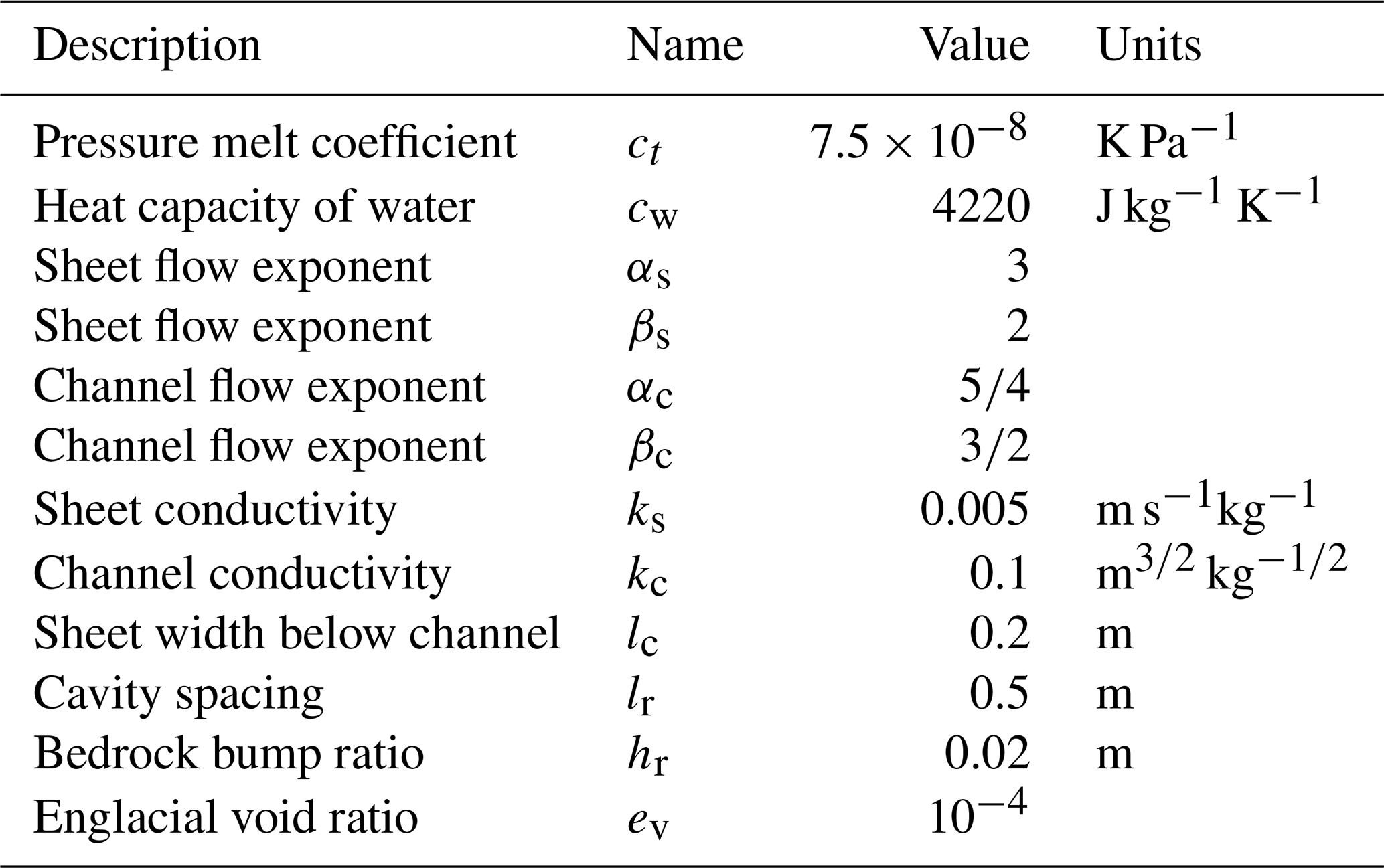
We use the GlaDS module of Elmer/Ice (Gagliardini and Werder, 2018) to model Hansbreen subglacial hydrology. GlaDS simulates both inefficient distributed drainage, represented by a sheet of water that covers the whole area of the glacier, and efficient channelized drainage, represented by a series of channels generated on the edges of the mesh elements of the domain (see more detail in Werder et al., 2013). The implementation of the hydrological model for this work has been adapted, regarding the size of our domain, following Gagliardini and Werder (2018) and Cook et al. (2020). The main parameters of the model are set out in Table 1.
We use GlaDS to obtain subglacial discharge estimates at the grounding line. Therefore, it is run at the bed of the glacier using the same mesh as the ice model to avoid complexity. Water is not permitted to flow through the lateral boundaries, and we set the hydraulic potential, ϕ, to zero at the grounding line. From Eq. (2) combined with the definition of the hydraulic potential, we obtain
Water entering the hydrological system is derived from surface and basal meltwater production. Surface melting is determined by calculating monthly averages for the surface meltwater, assuming it travels directly to the bed at the same point of production at the surface. As for basal meltwater, we suppose a distributed melt calculated using a geothermal heat flux of 63 mW m−2 (Gagliardini and Werder, 2018).
2.2.4 Plume model
In this work we use a plume model implemented in Elmer/Ice (Cook et al., 2020, 2022) based on buoyant plume theory (Jenkins, 2011; Slater et al., 2015). In that model, a continuous sheet-style line plume, split into coterminous segments, is simulated across the calving front. The field studies carried out on tidewater glaciers (Fried et al., 2015; Jackson et al., 2017) justify the choice of this plume geometry.
The plume model is initialized by the subglacial discharge at each node of the grounding line, where the subglacial discharge values are obtained as a solution of the subglacial hydrology model. Due to the density differences between meltwater and fjord water, subglacial discharge water rises in contact with the calving front, mixing turbulently with the surrounding water and producing melting at the ice–water interface. The calculated melt rates are then applied to modify the geometry of the submerged part of the calving front.
2.2.5 Model design
This model is implemented in 30 d monthly cycles that are run sequentially to cover the total simulation time, September 2008 to March 2011. The selection of this period is determined by the observational data. The simulation starts in September 2008, which is the date of the available surface DEM, but the first 6 months is considered to be the initialization of the model. Beyond March 2011, there are no surface velocity data available. Every cycle is divided into three steps (Fig. 3) as follows.
-
Inversion for the slip coefficient. An inversion using adjoint methods (Gillet-Chaulet et al., 2012) is performed to adjust the slip coefficient to the changing mean velocities for a given month. This is done by minimizing a cost function for the velocities, running monthly steady-state simulations. It is performed monthly to account for the changes in the velocity field while keeping a reasonable computational cost.
-
Dynamical and hydrological models and free-surface evolution. From the inversion results, the hydrology is computed in a 30 d transient simulation with a 1 d time step. Subsequently, the daily subglacial discharge values are averaged over the month. At this point, the glacier surface is left to evolve freely, whereas the front remains fixed.
-
Calving and plume models' activation. The monthly averaged values of subglacial discharge and the fjord ambient conditions are the required input for the line plume model. The dynamic model is run again for a month with a 1 d time step but now with the modules for calving and plume enabled. In this case, the hydrology is not computed; the glacier surface is left to evolve freely; and the front is allowed to evolve as a combination of ice flow, submarine melting and calving. Therefore, each of these time steps results in a new glacier geometry and a new front position. To avoid a mesh degeneration that could cause critical problems to the model, a remeshing is performed either when calving occurs or after eight consecutive no-calving time steps.
The first cycle starts from the geometry described in Sect. 2.1, while every new cycle will start from the resulting geometry of the previous one.
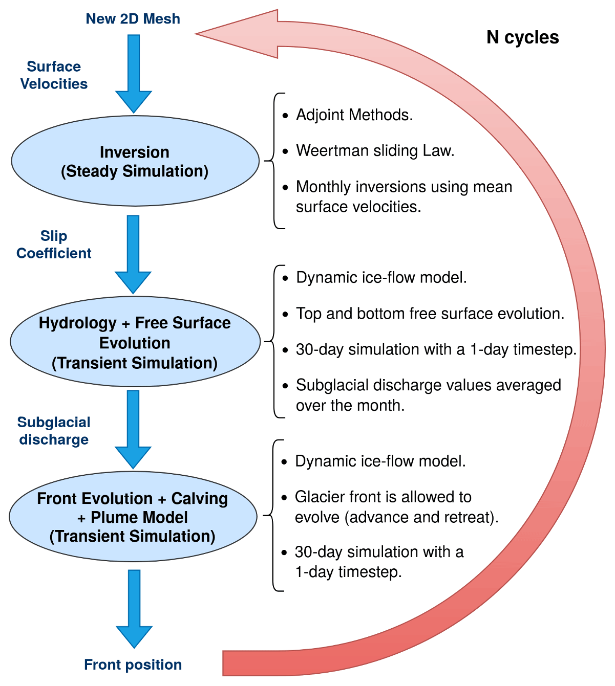
Figure 3Schematics of the three-step model procedure: inversion, dynamic model with hydrology module, and dynamic model with calving and plume modules. The red arrow indicates that a series of N cycles are run to cover the total simulation period.
Starting in March 2009, the modelled monthly values of surface meltwater, subglacial discharge, the plume melt rate and calving volume present a seasonal pattern (Fig. 4). The largest SMW values are reached in July (8.9 × 10⁵ and 8.3 × 10⁵ m3 a−1 for 2009 and 2010, respectively), and the cumulative SMW for both summer seasons is of the same order of magnitude, with the value for 2010 being ∼ 6 % lower than the one for 2009 (Fig. 4a). The largest subglacial discharge values are also reached in July (9.1 × 10⁵ and 5.7 × 10⁵ m3 a−1 for 2009 and 2010, respectively), but the total amount for both summer seasons varies significantly, by ∼ 25 % (Fig. 4c). Beyond the summer months, SMW and subglacial discharge maintain a baseline value around 1 × 10⁵ m3 a−1.
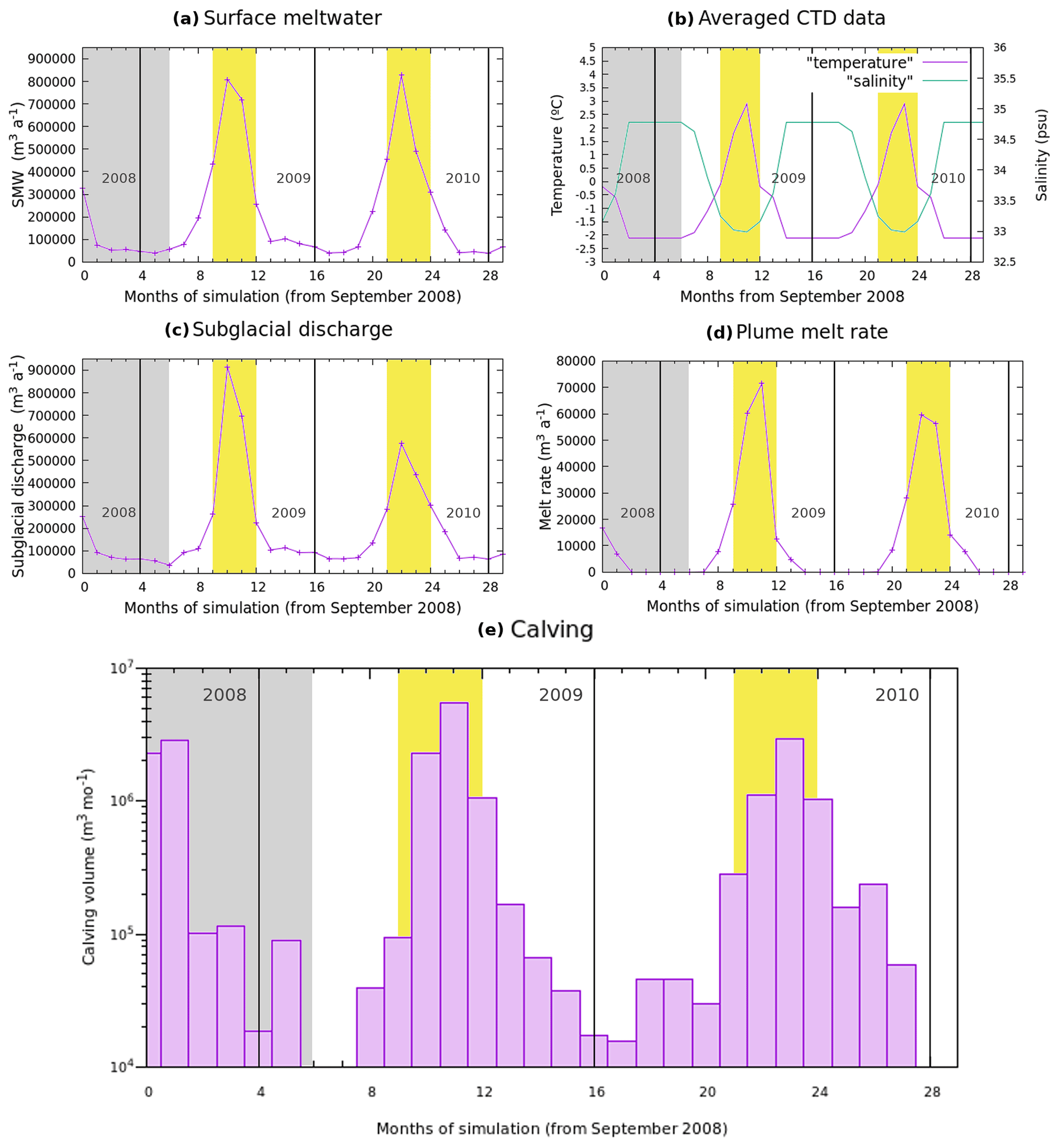
Figure 4Temporal evolution of the (a) surface meltwater (SMW), (b) average temperature and salinity of the fjord water near the calving front, (c) subglacial discharge produced by surface and basal melt, (d) total melt rate produced by plume activity computed on the first day of every month, and (e) calving volume produced by the model for every month of the simulation (log scale). The shaded areas correspond to the initialization period. The yellow areas indicate the summer periods, and the vertical black lines separate the different years.
The total melt rate due to plume activity presents a difference of ∼ 6 % between the two summer periods (1.7 × 10⁵ and 1.6 × 10⁵ m3 a−1 for 2009 and 2010, respectively). The largest plume melt rates for each summer period are reached in different months, August for 2009 (7.1 × 10⁴ m3 a−1) and July for 2010 (5.9 × 10⁴ m3 a−1) (Fig. 4d). Other than that, June presents values of around 2.6 × 10⁴ m3 a−1 and September of around 1.3 × 10⁴ m3 a−1. Note that no plume melt rate is produced from November to April, as no plumes are formed during these months.
Calving volume reaches the highest values in summer (Fig. 4e). The total calving volume during the first summer is considerably larger than during the second one, 8.89 × 10⁶ m3 per month versus 5.41 × 10⁶ m3 per month, and in the two cases the distribution presents some similarities: August is the month with the largest calving volume, 5.47 × 10⁶ m3 per month for 2009 and 2.97 × 10⁶ m3 per month for 2010; July comes in second with 2.28 × 10⁶ m3 per month for 2009 and 1.12 × 10⁶ m3 per month for 2010, almost half the volume of August in both cases; September exhibits values of around 1 × 10⁶ m3 per month in 2009 and 2010; and June presents the lowest values. The summer periods concentrate around 94 % of the calving volume (1.43 × 10⁷ m3 per month out of 1.52 × 10⁷ m3 per month), but calving occurs during the whole simulation except for in 4 months. Outside of the summer period, autumn months like October and November show moderate calving activity.
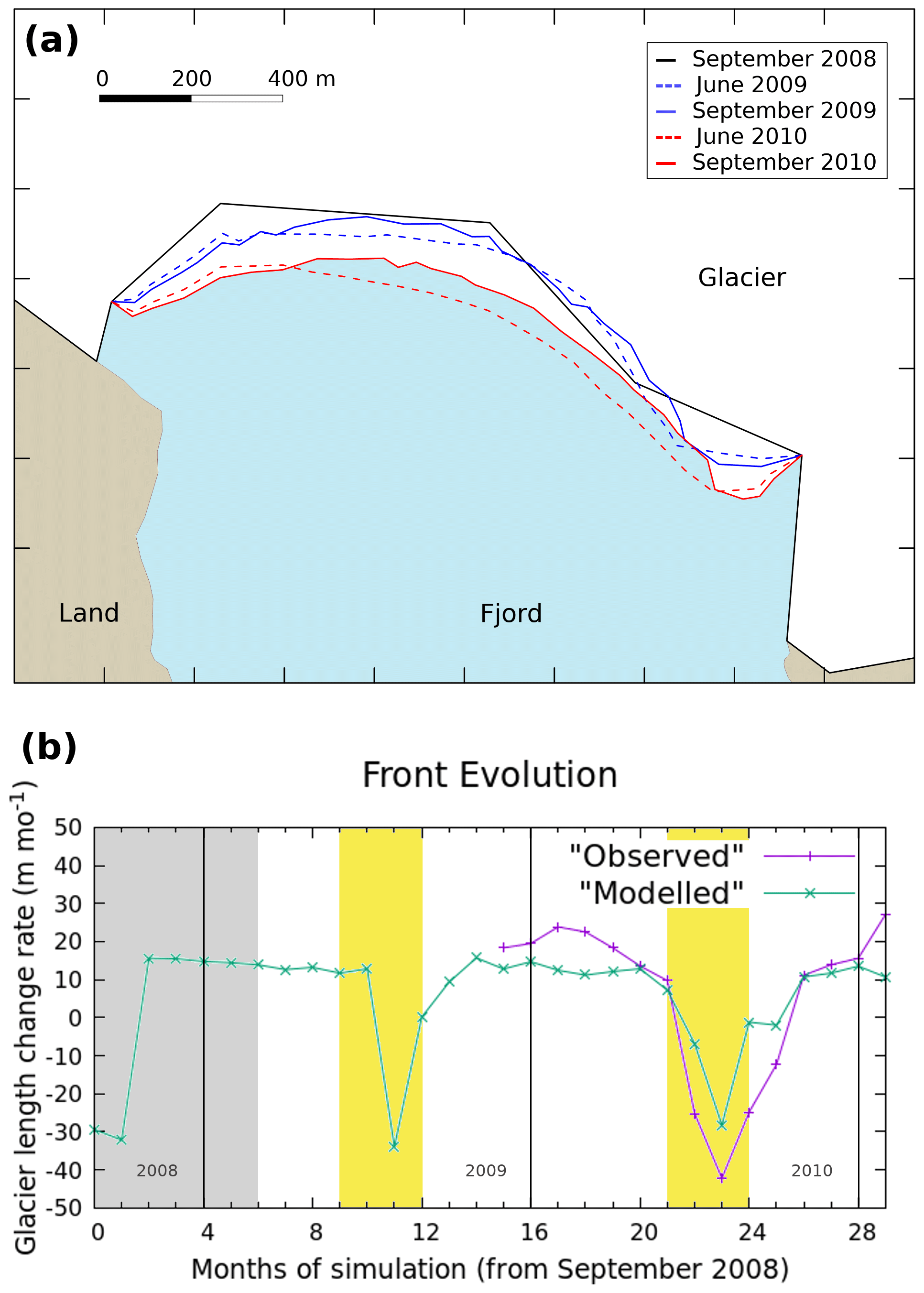
Figure 5Calving front evolution. (a) The different positions represent the interannual evolution and the summer evolution of the calving front: the solid lines correspond to September 2008 (black), September 2009 (blue) and September 2010 (red), whereas the dashed lines correspond to June 2009 (blue) and June 2010 (red). (b) The graph represents the longitudinal difference along the whole simulation, calculated as the difference in area between subsequent months divided by the glacier width. The shaded area corresponds to the initialization period. The yellow areas indicate the summer periods, and the vertical black lines separate the different years.
The calving front follows a seasonal pattern in terms of advance and retreat throughout the whole simulation period, generally retreating in summer and advancing during the rest of the year (Fig. 5b). The periods of advance are longer, and the advancing rate moves from 10 to 20 m per month of longitudinal difference, calculated as the difference in area between subsequent months divided by the glacier width. On the other hand, the periods of retreat are shorter and the retreating rate can reach up to −30 m per month. The largest negative values (indicating retreat) occur in August 2009 and 2010. The total advance is larger during the first year (March 2009–2010), 129.35 m per month, than in the second one (March 2010–2011), 89.98 m per month. As for cumulative retreat, in the first year this amounts to −33.94 m per month, whereas in the second one it is −38.23 m per month (Fig. 5a). By the end of the first year of simulation, March 2010, the front position has advanced 95.42 m per month with respect to the position in March 2009, while by the end of the second year of simulation, March 2011, the front position has advanced 51.74 m per month with respect to March 2010, resulting in a total advance of 147.16 m per month with respect to March 2009.
The results of the model indicate that the glacier presents a marked seasonal behaviour. Figures 2 and 4a and b exemplify this feature in the input data as well. Subglacial discharge values correlate with surface meltwater values (Fig. 4a, c). A constant value of basal and internal melting (∼ 2.6 × 10⁴ m3 a−1) has been applied using the geothermal heat flux defined in Sect. 2.2.3, which, along with some other processes like internal refreezing, explains why in some months the subglacial discharge is larger than the SMW. A 6 % decrease in SMW in summer 2010 was responsible for the 25 % decrease in subglacial discharge for the same period. However, this reduction in subglacial discharge cannot be fully attributed to the decrease in SMW. One possible explanation for this subglacial discharge reduction is a change in the efficiency of the drainage system that is not being captured by the model. This change would be consistent with the marked decrease in the velocity values at the beginning of summer 2010 (Fig. 2b).
The plume melt rate is affected by both fjord ambient conditions and subglacial discharge. The model calculates non-zero freshwater flux into the fjord in winter months (Fig. 4c), in agreement with Cook et al. (2020). However, in the present study, either the subglacial discharge values are not high enough or the winter ambient conditions are not suitable for the occurrence of plumes, unlike in the work of Cook et al. (2020) (Fig. 4d). This is a limitation of the model seeing as plumes have been observed at Hansbukta in winter. On the other hand, between April and October, both ambient conditions and subglacial discharge values are suitable for the occurrence of plumes. The ambient conditions in the fjord were kept the same for both summer periods. Hence, the differences between them can be explained by the differences in the subglacial discharge that feeds the plumes. As an exemplification, Fig. 6 shows two different distributions of the plume melt rate at the calving front: a high-melting month, August 2009 (panel a), and a low-melting month, October 2009 (panel b). Not only is the plume melt rate in August 2009 higher than the plume melt rate in October 2009, but also the melt extends to a larger area of the calving front. Comparing with other authors working on the same glacier–fjord system, the maximum melt rate values obtained for August 2010 are consistent with the ones obtained by De Andrés et al. (2018) (58 m3 per month versus 64.28 m3 per month (15 m3 per week)).
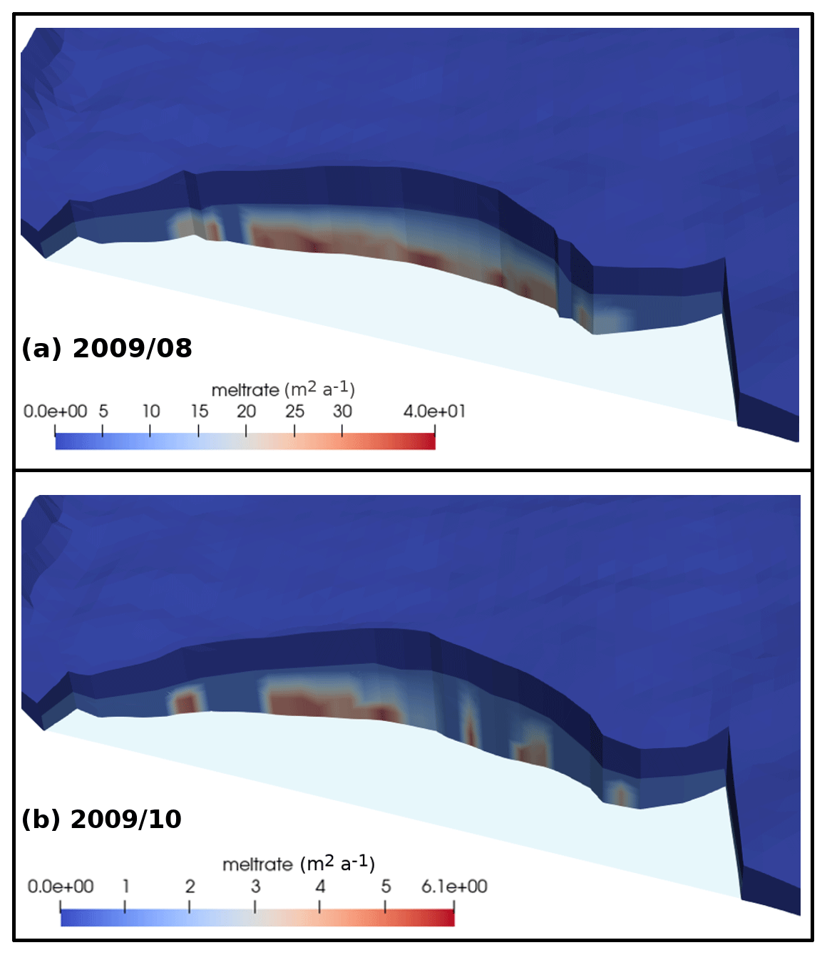
Figure 6A 3D aerial view of the glacier calving front for (a) August 2009 and (b) October 2009. The red zones represent high values of the melt rate due to plume activity, although the scales used are not the same. Different scales have been chosen to account for the significant differences between the values.
As for the calving volume, the total amount in the first year of simulation is significantly larger than in the second one, 9.24 × 10⁶ m3 per month versus 5.98 × 10⁶ m3 per month. This is consistent with the higher values of the plume melt rate during the first year, especially in August. From the results of this model it is not possible to establish an exact relation between plume melt rate and calving. For example, the plume melt rate in June 2010 is only slightly higher than that of June 2009, while the calving volume in June 2010 is more than twice that of June 2009. In September, however, a similar difference in plume melt rate (i.e. the melt rate in September 2010 is only slightly higher than that of September 2009) results in calving volumes of the same order of magnitude for both months (∼ 1 × 10⁶ m3 per month). Even so, in general, there is a clear correspondence between plume activity and calving, with the most intense plume activity consistently associated with the highest calving rates.
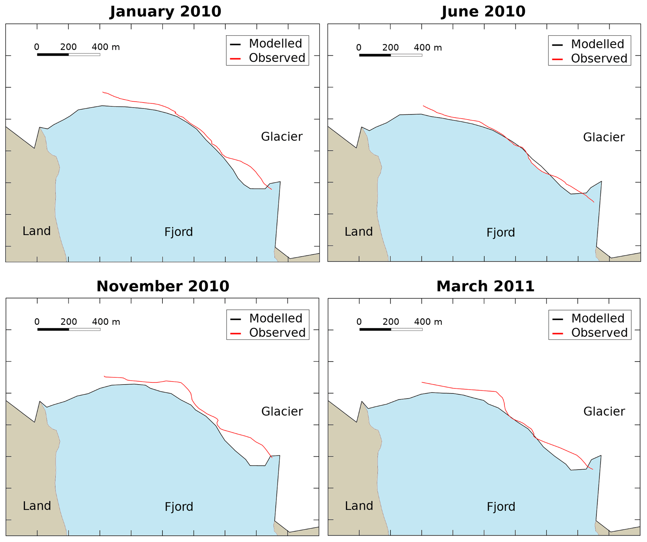
Figure 7A 2D aerial view of the glacier–fjord system for January 2010, June 2010, November 2010 and March 2011. The solid black lines represent the modelled contour of the glacier, and the red lines represent the observed front position. Note that the observational data do not cover the westernmost part of the front.
To study the evolution of the calving front and how it compares to the expected behaviour of a tidewater glacier, Fig. 5 outputs some interesting features. First of all, the glacier advances steadily during the winter months, when calving is not present in general, and retreats during the summer months, especially in August, when it reaches the highest absolute values. In general, the model is able to reproduce the seasonal tidewater glacier behaviour, since the modelled front evolution follows the same pattern as the observed one (Fig. 5b). However, both the advance and the retreat of the calving front are being underestimated. An explanation for the advance underestimation that is more than possible is the fact that the modelled velocities are generally lower than the observed ones (Fig. 2b), while calving underestimation is very likely to be the most important factor in the retreat dissimilarities. Secondly, calving is the main contributor to frontal ablation, but plume-induced melting can lead to a larger number of calving events, so both factors are important in the control of the front position. Finally, the glacier front remains quite stable during the study period (Fig. 5a). In fact, it shows a small advance between September 2008 and 2010, in agreement with Błaszczyk et al. (2021).
To validate the model performance, we also compare the modelled and observed front positions (Fig. 7). The modelled positions are in general more advanced than the observed ones. The difference between modelled and observed positions varies throughout the simulation. It starts with a decreasing period from December 2009 to July 2010. Afterwards, there is an increasing period from August 2010 to November 2010, followed by a final decrease until the end of the simulation in March 2011 (Fig. 8). There seems to be a seasonal pattern, but the lack of data beyond March 2011 does not allow us to establish such a thing. The results present a marked contrast between the central part and the east lateral margin of the glacier front, so the maximum differences in the eastern zone of the front are approximately 10 times larger than in the central one. This is likely due to the lack of calving events produced by the model in that region of the glacier front that could be caused by low plume-induced melting in the area. In general, the performance of the model is better when looking at only the central 350 m of the calving front. On average, the modelled positions are 40 % closer to the observed positions when taking just this central part (13.03 m versus 20.95 m for the total front), with half of the values below 10 m. Even so, in late spring and early summer, the differences in both cases, taking the whole calving front or just the central part, are considerably small and of the same order of magnitude.
Although a comparison between a 2D and a 3D model must be handled carefully, our results show a deviation of ±10 m for the central 350 m of the calving front between April and August 2010. This is the same as the deviation value obtained by De Andrés et al. (2018) for their flow-line model. To obtain those results, they needed to include a non-dimensional adjustable parameter used to parameterize the crevasse water depths (CWDs). In contrast, our model uses the 3D calving implementation of Todd et al. (2018), which ignores this process, so we do not need any CWD parameterization. Therefore, the inclusion of an across-glacier dimension extends the best results of the 2D model to the central 350 m of the calving front, where the 3D model predicts the observed front position with a good level of agreement. However, there is a region where the modelled positions are clearly behind the observed ones. The escalation of the difference coincides with the months when calving is larger at the glacier. Consequently, the cause of this increase could be, again, an underestimation of calving by the model. The reasons for this could be that the model is not able to capture all calving events occurring at the glacier or an underestimation of submarine melting, since higher values of submarine melting can enhance calving. Therefore these two factors have to be closely examined in order to improve the performance of the model.
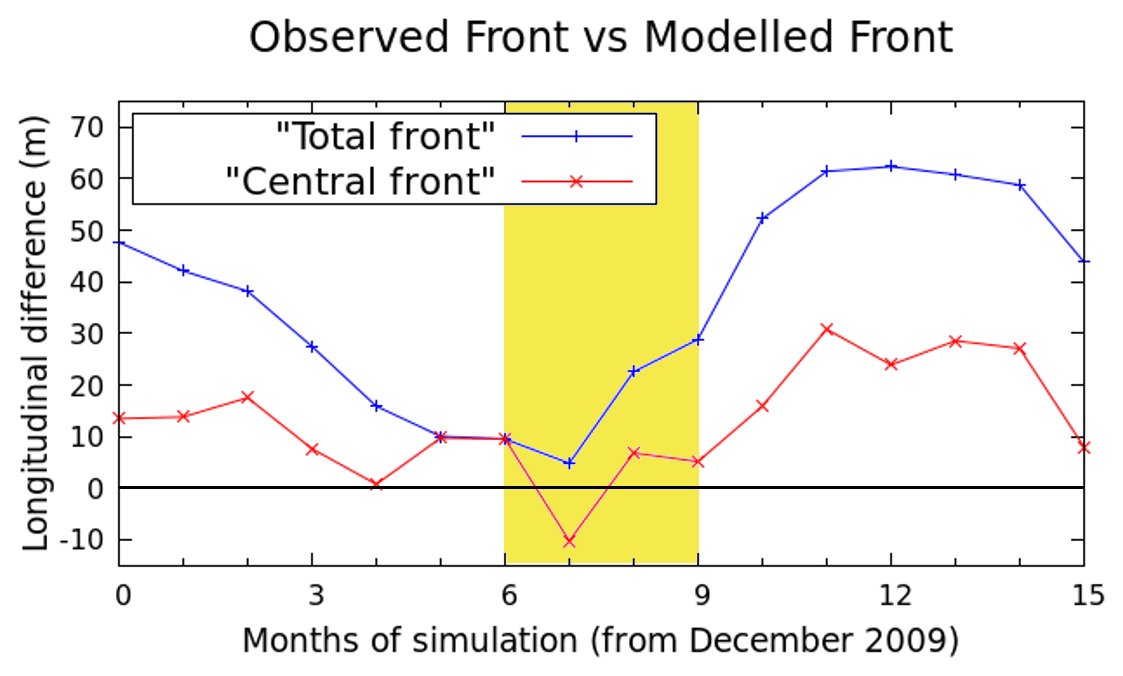
Figure 8Evolution of the longitudinal difference between the modelled and the observed front position calculated as the difference in area between them divided by the glacier width (blue line) and that same evolution restricted to the central 350 m of the calving front (red line). Positive values indicate that the modelled front is more advanced than the observed one, while negative values indicate the opposite. The zero is marked with a horizontal black line, so values closer to that line indicate a better agreement between modelled and observed positions. The yellow area indicates the summer period (June to September 2010).
Calving and frontal ablation are essential processes to take into account in our understanding of tidewater glacier dynamics. We have developed a 3D glacier dynamics model that, in addition to solve calving and subglacial hydrology, accounts for oceanic (by a plume model) and atmospheric (by surface mass balance and surface meltwater) factors too. Subglacial hydrology provides discharge values that, in combination with appropriate fjord ambient conditions, are high enough to generate plumes at the calving front except for during the coldest months, i.e. from November to April. The results for the hydrology are consistent with other studies using a similar model (Cook et al., 2020), while the results for the plume melt rate are in agreement with other works on the Hansbreen–Hansbukta glacier–fjord system (De Andrés et al., 2018).
The model is able to predict the evolution of the front position in terms of advance and retreat following a seasonal cycle with steep retreats in summer months and steady advances during the rest of the year. However, there are still differences between observed and modelled positions, especially in the eastern margin, where the longitudinal difference reaches 150 m in November 2010. In fact, when taking only the central part of the glacier front, the results improve significantly and the modelled positions become, on average, 40 % closer to the observed ones. In general, the difference between the modelled and observed front positions increases during the calving period, and we assume that the cause is an underestimation of calving by our model. Even so, the difference between the modelled and observed front positions decreases in some months, such as May, June and July. In these months, the model is able to predict the front position with a very good level of agreement. In the eastern margin, our model does not produce enough calving events, which causes that large difference. The timescale of this model is limited by the available data. We cannot say whether a longer simulation will result in a better agreement with observations; however, it would give us information on some results of the model that we cannot currently confirm. For example, do the differences in the eastern margin continue to increase or do they start to balance out and become shorter at some point? As the results seem to suggest, is there a seasonality in the differences such that they grow during the calving period and then decrease until reaching a minimum at the end of spring?
Changes in SMW alone are not able to explain plume behaviour, turning fjord ambient conditions into a key factor in this process. Additionally plume-induced melting has proven to be an essential factor for calving to occur. Consequently, a logical next step would be to use a fjord model to obtain better estimates of ambient conditions. Surface velocity calculation could also be reviewed in order to address the underestimation of the glacier change length rate during the periods of advance.
Finally, Hansbreen is a well-studied glacier, providing an essential context to test and to constrain our model. However, provided that we can count on having the required input data, this model could be applied to any other tidewater glacier or glacier–fjord system.
The data that support the results of this study and form the basis for all the figures presented in this paper are openly available via Zenodo at https://doi.org/10.5281/zenodo.8005258 (Muñoz-Hermosilla, 2023).
JMMH and JO designed the experiments. JMMH also developed the model code and executed the experiments with contributions from JO. EDA and KS provided surface mass balance and surface meltwater data. IPD and JO provided surface velocity data. JMMH analysed the model outputs and wrote the manuscript, with significant contributions from JO and FN. All authors contributed to and approved the final paper.
The contact author has declared that none of the authors has any competing interests.
Publisher’s note: Copernicus Publications remains neutral with regard to jurisdictional claims made in the text, published maps, institutional affiliations, or any other geographical representation in this paper. While Copernicus Publications makes every effort to include appropriate place names, the final responsibility lies with the authors.
Additional supporting field data were provided by the Hornsund Polish Polar Station. The authors thank Olivier Gagliardini, Tom Cowton and Peter Nienow for productive discussions as well as Samuel Cook for support with the Ice/Elmer model.
This research was carried out under project PID2020-113051RB-C31, funded by MCIN/AEI/10.13039/501100011033/ FEDER, UE, and grant PRE2018-084318, funded by MCIN/AEI/10.13039/501100011033 and the FSE “El FSE invierte en tu futuro”. Field measurements in Hornsund were supported by the Polish–Norwegian project AWAKE-2 (contract no. Pol–Nor/198675/17/2013).
This paper was edited by Josefin Ahlkrona and reviewed by two anonymous referees.
AMAP: Snow, Water, Ice and Permafrost in the Arctic (SWIPA), Arctic Monitoring and Assessment Programme (AMAP), Oslo, https://www.amap.no/documents/doc/snow-water-ice-and-permafrost-in-the-arctic-swipa-2017/1610 (last access: 24 January 2024), 2017. a
Amaral, T., Bartholomaus, T. C., and Enderlin, E. M.: Evaluation of iceberg calving models against observations from Greenland outlet glaciers, J. Geophys. Res.-Earth, 125, e2019JF005444, https://doi.org/10.1029/2019JF005444, 2020. a
Benn, D. I. and Åström, J.: Calving glaciers and ice shelves, Advances in Physics: X, 3, 1513819, https://doi.org/10.1080/23746149.2018.1513819, 2018. a
Benn, D. I., Warren, C. R., and Mottram, R. H.: “Calving laws”, “sliding laws” and the stability of tidewater glaciers, Ann. Glaciol., 46, 123–130, https://doi.org/10.3189/172756407782871161, 2007. a
Benn, D. I., Cowtom, T., Todd, J., and Luckman, A.: Glacier calving in Greenland, Curr. Clim. Change Rep., 3, 282–290, https://doi.org/10.1007/s40641-017-0070-1, 2017. a
Benn, D. I., Todd, J., Luckman, A., Bevan, S., Chudley, T. R., Åström, J., Zwinger, T., Cook, S., and Christoffersen, P.: Controls on calving at a large Greenland tidewater glacier: stress regime, self-organised criticality and the crevasse-depth calving law, J. Glaciol., 1–16, https://doi.org/10.1017/jog.2023.81, 2023. a
Błaszczyk, M., Jania, J. A., Ciepły, M., Grabiec, M., Ignatiuk, D., Kolondra, L., Kruss, A., Luks, B., Moskalik, M., Pastusiak, T., Strzelewicz, A., Walczowski, W., and Wawrzyniak, T.: Factors controlling terminus position of Hansbreen, a tidewater glacier in Svalbard, J. Geophys. Res.-Earth, 126, e2020JF005763, https://doi.org/10.1029/2020JF005763, 2021. a, b, c
Bojinski, S., M.Verstraete, Peterson, T. C., Richter, C., Simmons, A., and Zemp, M.: The concept of essential climate variables in support of climate research, applications, and policy, B. Am. Meteorol. Soc., 95, 1431–1443, https://doi.org/10.1175/BAMS-D-13-00047.1, 2014. a
Cassotto, R., Fahnestock, M., Amundson, J., Truffer, M., Boettcher, M., De la Peña, S., and Howat, I.: Non-linear glacier response to calving events, Jakobshavn Isbræ, Greenland, J. Glaciol., 65, 39–54, https://doi.org/10.1017/jog.2018.90, 2018. a
Church, J., Clark, P., Cazenave, A., Gregory, J., Jevrejeva, S., Levermann, A., Merrifield, M., Milne, G., Nerem, R. S., Nunn, P., Payne, A., Pfeffer, W. T., Stammer, D., and Alakkat, U.: Sea Level Change in: Climate Change 2013 – The Physical Science Basis. Contribution of Working Group I to the Fifth Assessment Report of the Intergovernmental Panel on Climate Change, edited by: Stocker, T. F., Qin, D., Plattner, G.-K., Tignor, M., Allen, S. K., Boschung, J., Nauels, A., Xia, Y., Bex V., and Midgley, P. M., in press, 1137–1216, https://doi.org/10.1017/CBO9781107415324, 2013. a
Cogley, J. G., Hock, R., Rasmussen, L. A., Arendt, A. A., Bauder, A., Braithwaite, R. J., Jansson, P., Kaser, G., Möller, M., Nicholson, L., and Zemp, M.: Glossary of glacier mass balance and related terms, IHP-VII Technical Documents in Hydrology No. 86, IACS Contribution No. 2, UNESCO-IHP, Paris, https://doi.org/10.5167/uzh-53475, 2011. a
Cook, S. J., Christoffersen, P., Todd, J., Slater, D., and Chauché, N.: Coupled modelling of subglacial hydrology and calving-front melting at Store Glacier, West Greenland , The Cryosphere, 14, 905–924, https://doi.org/10.5194/tc-14-905-2020, 2020. a, b, c, d, e, f, g, h
Cook, S. J., Chrostoffersen, P., and Todd, J.: A fully-coupled 3D model of a large Greenlandic outlet glacier with evolving subglacial hydrology, frontal plume melting and calving, J. Glaciol., 68, 486–502, https://doi.org/10.1017/jog.2021.109, 2022. a, b, c, d
Cownton, T. R., Slater, D. A., Sole, A., Goldberg, D., and Nienow, P.: Modeling the impact of glacial runoff on fjord circulation and submarine melt rate using a new subgrid-scale parameterization for glacial plumes, J. Geophys. Res.-Oceans, 120, 796–812, https://doi.org/10.1002/2014JC010324, 2015. a
Cownton, T. R., Todd, J. A., and Benn, D. I.: Sensitivity of tidewater glaciers to submarine melting governed by plume locations, Geophys. Res. Lett., 46, 11219–11227, https://doi.org/10.1029/2019GL084215, 2019. a
Cuffey, K. and Paterson, W. S. B.: The physics of glaciers, 4th edn., Elsevier, Elsevier, Oxford, ISBN 9780123694614, 2010. a
De Andrés, E., Otero, J., Navarro, F., Promińska, A., and Lapazaran, J.: A two-dimensional glacier–fjord coupled model applied to estimate submarine melt rates and front position changes of Hansbreen, Svalbard, J. Glaciol., 64, 745–758, https://doi.org/10.1017/jog.2018.61, 2018. a, b, c, d, e
De Andrés, E., Otero, J., Navarro, F., and Walczowski, W.: Glacier–plume or glacier–fjord circulation models? A 2-D comparison for Hansbreen–Hansbukta system, Svalbard, J. Glaciol., 67, 797–810, https://doi.org/10.1017/jog.2021.27, 2021. a, b
Edwards, T. L., Nowicki, S., Marzeion, B., Hock, R., Goelzer, H., Seroussi, H., Jourdain, N. C., Slater, D. A., Turner, F. E., Smith, C. J., McKenna, C. M., Simon, E., Abe-Ouchi, A., Gregory, J. M., Larour, E., Lipscomb, W. H., Payne, A. J., Shepherd, A., Agosta, C., Alexander, P., Albrecht, T., Anderson, B., Asay-Davis, X., Aschwanden, A., Barthel, A., Bliss, A., Calov, R., Chambers, C., Champollion, N., Choi, Y., Cullather, R., Cuzzone, J., Dumas, C., Felikson, D., Fettweis, X., Fujita, K., Galton-Fenzi, B. K., Gladstone, R., Golledge, N. R., Greve, R., Hattermann, T., Hoffman, M. J., Humbert, A., Huss, M., Huybrechts, P., Immerzeel, W., Kleiner, T., Kraaijenbrink, P., Le clec’h, S., Lee, V., Leguy, G. R., Little, C. M., Lowry, D. P., abd D. F. Martin, J. M., Da Maussion, F., Morlighem, M., O’Neill, J. F., Nias, I., Pattyn, F., Pelle, T., Price, S. F., Quiquet, A., Radić, V., Reese, R., Rounce, D. R., Rückamp, M., Sakai, A., Shafer, C., Schlegel, N., Shannon, S., abd F. Straneo, R. S. S., Sun, S., Tarasov, L., Trusel, L. D., Van Breedam, J., van de Wal, R., van den Broeke, M., Winkelmann, R., Zekollari, H., Zhao, C., Zhang, T., and Zwinger, T.: Projected land ice contributions to twenty-first-century sea level rise, Nature, 593, 74–82, https://doi.org/10.1038/s41586-021-03302-y, 2021. a, b
Finkelnburg, R.: Climate variability of Svalbard in the first decade of the 21st century and its impact on Vestfonna ice cap, Nordaustlandet, PhD Thesis, Technischen Universität Berlin, https://doi.org/10.14279/depositonce-3598, 2013. a
Fried, M. J., Catania, G. A., Bartholomaus, T. C., Duncan, D., Davis, M., Stearns, L. A., Nahs, J., Shroyer, E., and Sutherland, D.: Distributed subglacial discharge drives significant submarine melt at a Greenland tidewater glacier, Geophys. Res. Lett., 42, 9328–9336, https://doi.org/10.1002/2015GL065806, 2015. a
Gagliardini, O. and Werder, M.: Influence of increasing surface melt over decadal timescales on land-terminating Greenland-type outlet glaciers, J. Glaciol., 64, 700–710, https://doi.org/10.1017/jog.2018.59, 2018. a, b, c
Gagliardini, O., Zwinger, T., Gillet-Chaulet, F., Durand, G., Favier, L., de Fleurian, B., Greve, R., Malinen, M., Martín, C., Råback, P., Ruokolainen, J., Sacchettini, M., Schäfer, M., Seddik, H., and Thies, J.: Capabilities and performance of Elmer/Ice, a new-generation ice sheet model, Geosci. Model Dev., 6, 1299–1318, https://doi.org/10.5194/gmd-6-1299-2013, 2013. a
Gillet-Chaulet, F., Gagliardini, O., Seddik, H., Nodet, M., Durand, G., Ritz, C., Zwinger, T., Greve, R., and Vaughan, D. G.: Greenland ice sheet contribution to sea-level rise from a new-generation ice-sheet model, The Cryosphere, 6, 1561–1576, https://doi.org/10.5194/tc-6-1561-2012, 2012. a, b
Grabiec, M., Jania, J. A., Puczko, D., Kolondra, L., and Budzik, T.: Surface and bed morphology of Hansbreen, a tidewater glacier in Spitsbergen, Pol. Polar Res., 33, 111–138, https://api.semanticscholar.org/CorpusID:59475531 (last access: 24 January 2024), 2012. a, b
Hanna, E., Pattyn, F., Navarro, F., Favier, V., Goelzer, H., van den Broeke, M. R., Vizcaino, M., Whitehouse, P. L., Ritz, C., Bulthuis, K., and Smith, B.: Mass balance of the ice sheets and glaciers–progress since AR5 and challenges, Earth-Sci. Rev., 201, 102976, https://doi.org/10.1016/j.earscirev.2019.102976, 2020. a
Hewitt, I. J.: Subglacial plumes, Annu. Rev. Fluid Mech., 52, 145–169, https://doi.org/10.1146/annurev-fluid-010719-060252, 2020. a
Hock, R., Bliss, A., Marzeion, B., Giesen, R. H., Hirabayashi, Y., Huss, M., Radić, V., and Slangen, A. B. A.: GlacierMIP – A model intercomparison of global-scale glacier mass-balance models and projections, J. Glaciol., 65, 453–467, https://doi.org/10.1017/jog.2019.22, 2019. a
Holmes, F. A., Kirchner, N., Kuttenkeuler, J., Krützfeldt, J., and Noormets, R.: Relating ocean temperatures to frontal ablation rates at Svalbard tidewater glaciers: Insights from glacier proximal datasets, Sci. Rep., 9, 9442, https://doi.org/10.1038/s41598-019-45077-3, 2019. a
Hugonnet, R., McNabb, R., Berthier, E., Menounos, B., Nuth, C., Girod, L., Farinotti, D., Huss, M., Dussaillant, I., Brun, F., and Kääb, A.: Accelerated global glacier mass loss in the early twenty-first century, Nature, 592, 726–731, https://doi.org/10.1038/s41586-021-03436-z, 2021. a, b
Huss, M. and Hock, R.: A new model for global glacier change and sea-level rise, Front. Earth Sci., 3, 54, https://doi.org/10.3389/feart.2015.00054, 2015. a
Isaksen, K., Nordli, Ø., Førland, E. J., Łupikasza, E., Eastwood, S., and Niedźwiedź, T.: Recent warming on Spitsbergen – influence of atmospheric circulation and sea ice cover, J. Geophys. Res.-Atmos., 121, 11913–11931, https://doi.org/10.1002/2016JD025606, 2016. a
Jackson, R. H., Shroyer, E. L., Nash, J. D., Sutherland, D. A., Carroll, D., Fried, M. J., Catania, G. A., Bartholomaus, T. C., and Stearns, L. A.: Near-glacier surveying of a subglacial discharge plume: implications for plume parameterizations, Geophys. Res. Lett., 44, 6886–6894, https://doi.org/10.1002/2017GL073602, 2017. a, b
Jackson, R. H., Nash, J. D., Kienholz, C., Sutherland, D. A., Amundson, J. M., Motyka, R. J., Winters, D., Skyllingstad, E., and Pettit, E. C.: Meltwater intrusions reveal mechanisms for rapid submarine melt at a tidewater glacier, Geophys. Res. Lett., 47, e2019GL085335, https://doi.org/10.1029/2019GL085335, 2019. a
Jenkins, A.: A one-dimensional model of ice shelf-ocean interaction, J. Geophys. Res., 96, 671–677, 1991. a
Jenkins, A.: Convection-driven melting near the grounding lines of ice shelves and tidewater glaciers, J. Phys. Oceanogr., 41, 2279–2294, https://doi.org/10.1175/JPO-D-11-03.1, 2011. a, b
Jouvet, G., Weidmann, Y., Kneib, M., Detert, M., Seguinot, J., Sakakibara, D., and Sugiyama, S.: Short-lived ice speed-up and plume water flow captured by a VTOL UAV give insights into subglacial hydrological system of Bowdoin Glacier, Remote Sens. Environ., 17, 389–399, https://doi.org/10.1016/j.rse.2018.08.027, 2018. a
Kochtitzky, W., Copland, L., Van Wychen, W., Hugonnet, R., Hock, R., Dowdeswell, J. A., Benham, T., Strozzi, T., Glazovsky, A., Lavrentiev, I., Rounce, D. R., Millan, R., Cook, A., Dalton, A., Jiskoot, H., Cooley, J., Jania, J., and Navarro, F.: The unquantified mass loss of Northern Hemisphere marine-terminating glaciers from 2000–2020, Nat. Commun., 13, 5835, https://doi.org/10.1038/s41467-022-33231-x, 2022. a
Levermann, A., Albrecht, T., Winkelmann, R., Martin, M. A., Haseloff, M., and Joughin, I.: Kinematic first-order calving law implies potential for abrupt ice-shelf retreat, The Cryosphere, 6, 273–286, https://doi.org/10.5194/tc-6-273-2012, 2012. a
Luckman, A., Benn, D. I., Cottier, F., Bevan, S., Nilsen, F., and Inall, M.: Calving rates at tidewater glaciers vary strongly with ocean temperature, Nat. Commun., 6, 8566, https://doi.org/10.1038/ncomms9566, 2015. a
Masson-Delmotte, V., Zhai, P., Pirani, A., Conners, S., Péan, C., Berger, S., Caud, N., Chen, Y., Goldfarb, L., Gomis, M. I., Huang, M., Leitzell, K., Lonnoy, E., Matthews, J. B. R., Maycock, T. K., Waterfield, T., Yelekçi, O., Yu, R., and Zhou, B. (Eds.): IPCC Climate Change 2021: The Physical Science Basis. Contribution of Working Group I to the Sixth Assessment Report of the Intergovernmental Panel on Climate Change, Cambridge University Press, Cambridge, UK and New York, NY, USA, https://doi.org/10.1017/9781009157896, 2021. a
Meier, M. F., , Dyurgerov, M. B., Rick, U. K., O'neel, S., Pfeffer, W. T., Anderson, R. S., Anderson, S. P., and Glazovsky, A. F.: Glaciers dominate eustatic sea-level rise in the 21st century, Science, 317, 1064, https://doi.org/10.1126/science.1143906, 2007. a
Mercenier, R., Lüthi, M. P., and Vieli, A.: Calving relation for tidewater glaciers based on detailed stress field analysis, The Cryosphere, 12, 721–739, https://doi.org/10.5194/tc-12-721-2018, 2018. a
Morlighem, M., Bondzio, J., Seroussi, H., Rignot, E., Larour, E., Humbert, A., and Rebuffi, S.: Modeling of Store Gletscher's calving dynamics, West Greenland, in response to ocean thermal forcing, Geophys. Res. Lett., 43, 2659–2666, https://doi.org/10.1002/2016GL067695, 2016. a
Morton, B. R., Taylor, G., and Turner, J. S.: Turbulent gravitational convection from maintained and instantaneous sources, Proceedings of the Royal Society A: Mathematical, Physical and Engineering Sciences, 234, 1–23, https://doi.org/10.1098/rspa.1956.0011, 1956. a
Motyka, R. J., Dryer, W. P., Amundson, J., Truffer, M., and Fahnestock, M.: Rapid submarine melting driven by subglacial discharge, LeConte Glacier, Alaska, Geophys. Res. Lett., 40, 5153–5158, https://doi.org/10.1002/grl.51011, 2013. a
Möller, M., Navarro, F., Huss, M., and Marzeion, B.: Projected sea-level contributions from tidewater glaciers are highly sensitive to chosen bedrock topography: A case study at Hansbreen, Svalbard, J. Glaciol., 69, 966–980, https://doi.org/10.1017/jog.2022.117, 2023. a
Muñoz-Hermosilla, J. M.: A 3D glacier dynamics-line plume model to estimate the frontal ablation of Hansbreen, Zenodo [data set], https://doi.org/10.5281/zenodo.8005258, 2023. a
Navarro, F. J., Martín-Español, A., Lapazaran, J. J., Grabiec, M., Otero, J., Vasilenko, E. V., and Puczko, D.: Ice volume estimates from Ground-Penetrating Radar surveys, Wedel Jarlsberg Land Glaciers, Svalbard, Arct. Antarct. Alp. Res., 46, 394–406, https://doi.org/10.1657/1938-4246-46.2.394, 2014. a
Nick, F. M., Van der Veen, C., Vieli, A., and Benn, D. I.: A physically based calving model applied to marine outlet glaciers and implications for the glacier dynamics, J. Glaciol., 56, 781–794, https://doi.org/10.3189/002214310794457344, 2010. a
Nordli, Ø., Wyszyński, P., Gjelten, H. M., Isaksen, K., Łupikasza, E., Niedźwiedź, T., and Przybylak, R.: Revisiting the extended Svalbard Airport monthly temperature series, and the compiled corresponding daily series 1898–2018, Polar Res., 39, https://doi.org/10.33265/polar.v39.3614, 2020. a
Oerlemans, J., Jania, J., and Kolondra, L.: Application of a minimal glacier model to Hansbreen, Svalbard, The Cryosphere, 5, 1–11, https://doi.org/10.5194/tc-5-1-2011, 2011. a
Otero, J., Navarro, F. J., Martin, C., Cuadrado, M. L., and Corcuera, M.: A three-dimensional calving model: numerical experiments on Johnsons Glacier, Livingston Island, Antarctica, J. Glaciol., 56, 200–214, https://doi.org/10.3189/002214310791968539, 2010. a
Otero, J., Navarro, F. J., Lapazaran, J. J., Welty, E., Puczko, D., and Finkelnburg, R.: Modeling the controls on the front position of a tidewater glacier in Svalbard, Front. Earth Sci., 5, 29, https://doi.org/10.3389/feart.2017.00029, 2017. a, b
Perez-Doña, I. and Otero, J.: Sobre el uso de Kriging Bayesiano para estimar la evolución de las velocidades en superficie del Glaciar Hansbreen (Svalbard), in: 10a Asamblea Hispano-Portuguesa de Geodesia y Geofísica, Spain, 28 November–1 December 2022, 1137–1140, https://doi.org/10.7419/162.07.2023, 2023. a
Pętlicki, M., Ciepły, M., Jania, J., Promińska, A., and Kinnard, C.: Calving of a tidewater glacier driven by melting at the waterline, J. Glaciol., 61, 851–863, https://doi.org/10.3189/2015JoG15J062, 2015. a
Rignot, E., Koppes, M., and Velicogna, I.: Rapid submarine melting of the calving faces of west Greenland glacier, Nat. Geosci., 3, 187–191, https://doi.org/10.1038/ngeo765, 2010. a
Slater, D. A., Nienow, P., Cownton, T. R., Goldberg, D., and Sole, A.: Effect of near-terminus subglacial hydrology on tidewater glacier submarine melt rates, Geophys. Res. Lett., 42, 2861–2868, https://doi.org/10.1002/2014GL062494, 2015. a, b
Slater, D. A., Straneo, F., Das, S. B., Richards, C. G., Wagner, T. J. W., and Nienow, P. W.: Localized plumes drive front-wide ocean melting of a Greenlandic tidewater glacier, Geophys. Res. Lett., 45, 12350–12358, https://doi.org/10.1029/2018GL080763, 2018. a
Straneo, F. and Cenedese, C.: The dynamics of Greenland's glacial fjords and their role in climate, Annu. Rev. Mar. Sci, 7, 89–112, https://doi.org/10.1146/annurev-marine-010213-135133, 2015. a
Sutherland, D. A., Jackson, R. H., Kienholz, C., Amundson, J. M., Dryer, W. P., Duncan, D., Eidam, E. F., Motyka, R. J., and Nash, J. D.: Direct observations of submarine melt and subsurface geometry at a tidewater glacier, Science, 365, 369–374, https://doi.org/10.1126/science.aax3528, 2019. a
Todd, J. and Christoffersen, P.: Are seasonal calving dynamics forced by buttressing from ice mélange or undercutting by melting? Outcomes from full-Stokes simulations of Store Glacier, West Greenland, The Cryosphere, 8, 2353–2365, https://doi.org/10.5194/tc-8-2353-2014, 2014. a
Todd, J., Christoffersen, P., Zwinger, T., Råback, P., Chauché, N., Benn, D., Luckman, A., Ryan, J., Toberg, N., Slater, D., and Hubbard, A.: A full-Stokes 3D calving model applied to a large greenlandic glacier, J. Geophys. Res.-Earth Surf., 123, 410–432, https://doi.org/10.1002/2017JF004349, 2018. a, b, c, d
Todd, J., Christoffersen, P., Zwinger, T., Råback, P., and Benn, D. I.: Sensitivity of a calving glacier to ice–ocean interactions under climate change: new insights from a 3-D full-Stokes model, The Cryosphere, 13, 1681–1694, https://doi.org/10.5194/tc-13-1681-2019, 2019. a, b
Vallot, D., Adinugroho, S., Strand, R., How, P., Pettersson, R., Benn, D. I., and Hulton, N. R. J.: Automatic detection of calving events from time-lapse imagery at Tunabreen, Svalbard, Geosci. Instrum. Method. Data Syst., 8, 113–127, https://doi.org/10.5194/gi-8-113-2019, 2019. a
Van der Veen, C.: Tidewater calving, J. Glaciol., 42, 375–385, https://doi.org/10.3189/S0022143000004226, 1996. a
Vieli, A., Funk, M., and Blatter, H.: Tidewater glaciers: Frontal flow acceleration and basal sliding, Ann. Glaciol., 31, 217–221, https://doi.org/10.3189/172756400781820417, 2000. a
Vieli, A., Funk, M., and Blatter, H.: Flow dynamics of tidewater glaciers: A numerical modelling approach, J. Glaciol., 47, 595–606, https://doi.org/10.3189/172756501781831747, 2001. a
Vieli, A., Jania, J., and Kolondra, L.: The retreat of a tidewater glacier: Observations and model calculations on Hansbreen, Spitsbergen, J. Glaciol., 48, 592–600, https://doi.org/10.3189/172756502781831089, 2002. a
Werder, M. A., Hewitt, I. J., Schoof, C. G., and Flowers, G. E.: Modeling channelized and distributed subglacial drainage in two dimensions, J. Geophys. Res.-Earth, 118, 21402158, https://doi.org/10.1002/jgrf.20146, 2013. a, b
Xie, S., Dixon, T. H., Holland, D. M., Voytenko, D., and Vaňková, I.: Rapid iceberg calving following removal of tightly packed pro-glacial mélange, Nat. Commun., 10, 3250, https://doi.org/10.1038/s41467-019-10908-4, 2019. a