Validation of pan-Arctic soil temperatures in modern reanalysis and data assimilation systems

Reanalysis products provide spatially homogeneous coverage for a variety of climate variables in regions such as the Arctic where observational data are limited. Soil temperatures are an important control of many land–atmosphere exchanges and hydrological processes, and permafrost soils are thawing as the climate warms. However, very little validation of reanalysis soil temperatures in the Arctic has been performed to date, because widespread in situ reference observations have historically been limited there. Here we validate pan-Arctic soil temperatures from eight reanalysis and land data assimilation system products, using a newly assembled database of in situ observations from diverse measurement networks across Eurasia and North America. We examine product performance across the extratropical Northern Hemisphere between 1982 and 2018, and find that most products have soil temperatures that are biased cold by 1–5 K, with an RMSE of 2–9 K, and that biases and RMSE are generally largest in the cold season. Monthly mean values from most products correlate well with in situ data (r>0.9) in the warm season but show lower correlations (r=0.55–0.85) in the cold season. Similarly, the magnitude of monthly variability in soil temperatures is well captured in summer but overestimated by 20 %–50 % for several products in winter. The suggestion is that soil temperatures in reanalysis products are subject to much higher uncertainty when the soil is frozen and/or when the ground is snow covered, suggesting that the representation of processes controlling snow cover in reanalysis systems should be urgently studied. We also validate the ensemble mean of all available products and find that, when all seasons and metrics are considered, the ensemble mean generally outperforms any individual product, in terms of its correlation and variability, while maintaining relatively low biases. As such, we recommend the ensemble mean soil temperature product for a wide range of applications, such as the validation of soil temperatures in climate models, and to inform models that require soil temperature inputs, such as hydrological models.

1 Introduction

Soil temperatures, both near the surface and at depth, are an important control of many physical, hydrological, and land surface processes, as soils act as a reservoir for energy and moisture underground. They provide an important initial condition for numerical weather prediction, as energy and water fluxes from the land are important for convective processes (Dirmeyer et al., 2006; Kim and Wang, 2007; Siqueira et al., 2009). As soils react relatively slowly to variations in weather, soil temperature is also an important predictor of seasonal and mid-term weather forecasts (Xue et al., 2011). Soils over large portions of the Arctic are perennially frozen (permafrost soil). Roughly 1400–1600 Gt of carbon are estimated to be stored in soils in permafrost-affected regions of the Northern Hemisphere (Hugelius et al., 2014). Continued warming and thawing of permafrost soils as well as related decomposition of carbon could act as a potential positive feedback on warming – the permafrost carbon feedback – by releasing more methane (CH₄) and carbon dioxide (CO₂) into the atmosphere (Koven et al., 2011). In situ based soil temperature monitoring networks using thermistor probes, particularly at high latitudes, are limited in terms of their spatial and temporal coverage (Yi et al., 2019), making it difficult to assess hemispheric scale changes in permafrost.

Reanalysis products have been used in a variety of weather and climate applications to provide information on a regular spatial grid, particularly in regions where limited or no observational data are available (Koster et al., 2004; Zhang et al., 2008). Previous studies validating reanalysis soil temperature have primarily focused on the middle latitudes, such as across China (Yang and Zhang, 2018; Zhan et al., 2020; Zhao et al., 2022), the Qinghai–Tibetan Plateau (Hu et al., 2019; Jiao et al., 2023; Wu et al., 2018), Europe (Albergel et al., 2015; Johannsen et al., 2019), and the continental United States (Albergel et al., 2015; Xia et al., 2013), with a couple of recent studies validating soil temperatures globally (Li et al., 2020; Cao et al., 2020; Ma et al., 2021). Relative to in situ ground temperature probe networks, most reanalysis products are biased cold by about 2–5 °C, on average (Hu et al., 2019; Qin et al., 2020; Yang and Zhang, 2018). Ma et al. (2021) found that most reanalysis products show larger cold biases over polar regions than they do over tropical and temperate regions, while a recent study by Cao et al. (2020) found that ERA5-Land soil temperatures were biased warm over the Arctic, particularly in winter.

Several explanations have been suggested for the biases in reanalysis soil temperatures, including model parameterizations (Albergel et al., 2015; Cao et al., 2020; Chen et al., 2015; Wu et al., 2018; Xiao et al., 2013), air temperature biases (Cao et al., 2020; Hu et al., 2017), errors in topography and elevation, arising from the coarse resolution of reanalysis products (Yang and Zhang, 2018; Zhao et al., 2008; Ma et al., 2021), and errors in simulated snow cover and snow thermal insulation (Cao et al., 2020; Royer et al., 2021; Cao et al., 2022).

While soil temperature biases in individual reanalysis products may limit their utility, a consensus is emerging that multi-product ensembles, based on the same principle as ensemble weather prediction (World Meteorological Organization, 2012), are an effective way to increase the signal-to-noise ratio for many important geophysical variables. Ensemble mean datasets based on combinations of in situ, model, satellite, and reanalysis data have been used to reduce biases in estimates of snow water equivalent (Mudryk et al., 2015), soil moisture (Dorigo et al., 2017; Gruber et al., 2019), and precipitation (Beck et al., 2019), as well as for local-scale permafrost simulations (Cao et al., 2019). Li et al. (2020) suggest that a similar method could be used to reduce biases in reanalysis soil temperatures.

Reanalysis soil temperatures have been relatively well characterized over the middle latitudes. Studies validating Arctic soil temperatures in reanalysis products, however, have either focused on a single product (Cao et al., 2020) or have only considered a limited spatial extent (Li et al., 2020; Ma et al., 2021). Here we perform a validation of pan-Arctic (and Boreal) soil temperatures from eight reanalysis and land data assimilation system (LDAS) products. The main objectives are to (1) validate the eight reanalysis and LDAS soil temperature products in terms of their bias, RMSE, correlation, and standard deviation, and (2) investigate whether an ensemble mean soil temperature product outperforms the individual reanalysis products.

2 Data

2.1 Reanalysis and LDAS data

Tables 1 and 2 outline the six reanalysis and two LDAS soil temperature products used in this study. For simplicity, the term “reanalysis” will hereafter be used to describe both reanalysis and LDAS products. A summary of each product follows below. Products were remapped onto the European Reanalysis – Interim (ERA-Interim) grid for comparison using three different methods: nearest-neighbour, bilinear interpolation, and first-order conservative remapping. The choice of remapping method did not affect the overall conclusions of the study, and the analysis is based on data remapped using the conservative remapping method, as it facilitated the use of the largest number of validation sites and grid cells.

The reanalysis products investigated span a wide range of horizontal resolutions, ranging between 0.1°, in the case of ERA5-Land and FLDAS, to 0.75° for ERA-Interim (Table 1). Most products – CFSR, ERA-Interim, ERA5, ERA5-Land, and the Famine Early Warning Systems Network Land Data Assimilation System (FLDAS) – simulate soil temperature across four vertical layers, while MERRA2 includes six vertical layers and JRA55 calculates soil temperature across a single layer. The topmost soil layer has the highest resolution (7–10 cm in most cases), while the bottom soil layer often averages soil properties over 1 m or more (Table 2).

The Noah Land Surface Model (Noah-LSM) (Chen et al., 1996; Betts et al., 1997; Koren et al., 1999; Ek, 2003) is used by CFSR and FLDAS. CFSR uses the Noah-LSM in a fully coupled mode to obtain a first-guess land–atmosphere simulation before operating in a semi-coupled mode with GLDAS to obtain information about the state of the land surface (Saha et al., 2010a). FLDAS, however, is run in an offline mode utilizing meteorological forcing from MERRA2 (McNally et al., 2017) and rainfall information from NOAA's Global Data Assimilation (GDAS) (Derber et al., 1991), the Climate Hazards Group Infrared Precipitation with Stations (CHIRPS) (Funk et al., 2015), and the African Rainfall Estimation version 2.0 (RFE2) (Xie and Arkin, 1997).

ERA-Interim, ERA5, and ERA5-Land use versions of the Tiled ECMWF Scheme for Surface Exchanges over Land (TESSEL) land model (Viterbo and Beljaars, 1995; Viterbo and Betts, 1999). In the case of ERA-Interim, TESSEL is informed by empirical corrections from 2 m (surface) air temperature and humidity (Dee et al., 2011). Meanwhile, ERA5 and ERA5-Land use an updated version of TESSEL, known as the Hydrology-Tiled ECMWF Scheme for Surface Exchanges over Land (HTESSEL) (Balsamo et al., 2009). In ERA5, a weak coupling exists between the land surface and atmosphere. It includes an advanced LDAS that incorporates information regarding the near-surface air temperature, relative humidity, as well as snow cover (de Rosnay et al., 2014), along with satellite estimates of soil moisture and soil temperature from the top 1 m of soil (de Rosnay et al., 2013). ERA5-Land, unlike ERA5, does not directly assimilate observational data. Instead, the ERA5 meteorology (such as air temperature, humidity, and atmospheric pressure) is used as forcing information for HTESSEL, allowing it to be run at higher resolutions (Muñoz-Sabater et al., 2021). It includes an improved parameterization of soil thermal conductivity allowing for it to account for ice content in frozen soil, improvements to soil water balance conservation, and the ability to capture rain-on-snow events (Muñoz-Sabater et al., 2021).

MERRA2 utilizes the Catchment Land Surface Model (CLSM) (Ducharne et al., 2000; Koster et al., 2000). Though MERRA2 does not include a land surface analysis (Gelaro et al., 2017), CLSM is informed using an updated version of the Climate Prediction Center's unified gauge-based analysis of global daily precipitation (CPCU) precipitation correction algorithm that originated in MERRA-Land (Reichle et al., 2017b). No corrections are available, however, for high latitude regions north of 62.5° N (Reichle et al., 2017a). Finally, JRA55 uses the Simple Biosphere Model (SiB) (Onogi et al., 2007; Sato et al., 1988; Sellers et al., 1986) in offline mode, forced by atmospheric data and data from land surface analyses that incorporate microwave satellite retrievals of snow cover (Kobayashi et al., 2015).

Saha et al. (2010a)Saha et al. (2014)Hersbach et al. (2020)Muñoz-Sabater et al. (2021)Dee et al. (2011)McNally et al. (2017)Harada et al. (2016)Kobayashi et al. (2015)Gelaro et al. (2017)

Table 1 Summary of the eight reanalysis and LDAS products, their equatorial resolution, land model, and relevant references.

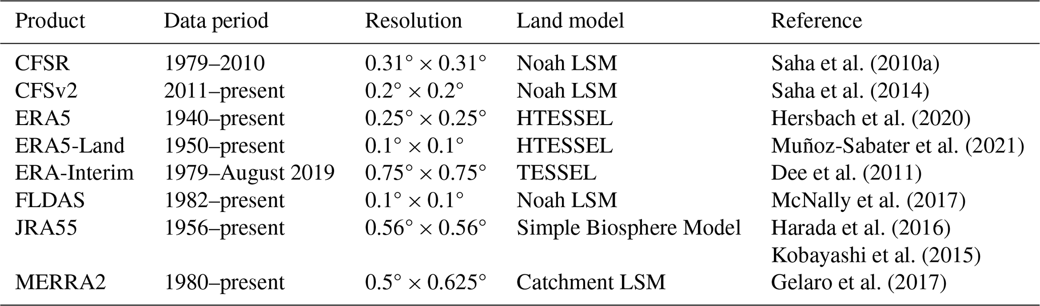
Table 2 Summary of the eight reanalysis and LDAS products, as well as the number and depths of the soil layers included.

^* The JRA55 Simple Biosphere Model contains up to three soil layers (whose depths vary depending on vegetation type), but the soil temperature is averaged over all layers to produce a singular value at each grid cell.

2.2 Observational data

Owing to the lack of dense soil temperature monitoring networks in the Arctic, most of the observed soil temperature record is characterized by a soil temperature record that is temporally and spatially sparse (Luo et al., 2020). While Russia has a more complete record of permafrost temperatures extending back to the 1980s (Sherstiukov, 2012), longer-term permafrost records over North America are generally limited to the western Arctic (Smith et al., 2010). Portions of coastal Nunavik, in northern Quebec, have records of permafrost temperatures from the 1990s onwards (CEN, 2020a, b, c, d, e, f, g), while soil temperature measurements in the central Arctic are rather sparse (Smith et al., 2010). Rather than limit our validation to a small geographic region in the permafrost zone, as several prior studies have done (Hu et al., 2019; Qin et al., 2020; Wu et al., 2018; Ma et al., 2021; Li et al., 2020), we choose to combine data from a variety of sparse and dense networks. Such an approach has been used to validate soil temperature and permafrost performance in ERA5-Land (Cao et al., 2020), and allows for the examination of larger geographic regions as well as for the inclusion of a more diverse set of vegetation types across the continent (Ma et al., 2021).

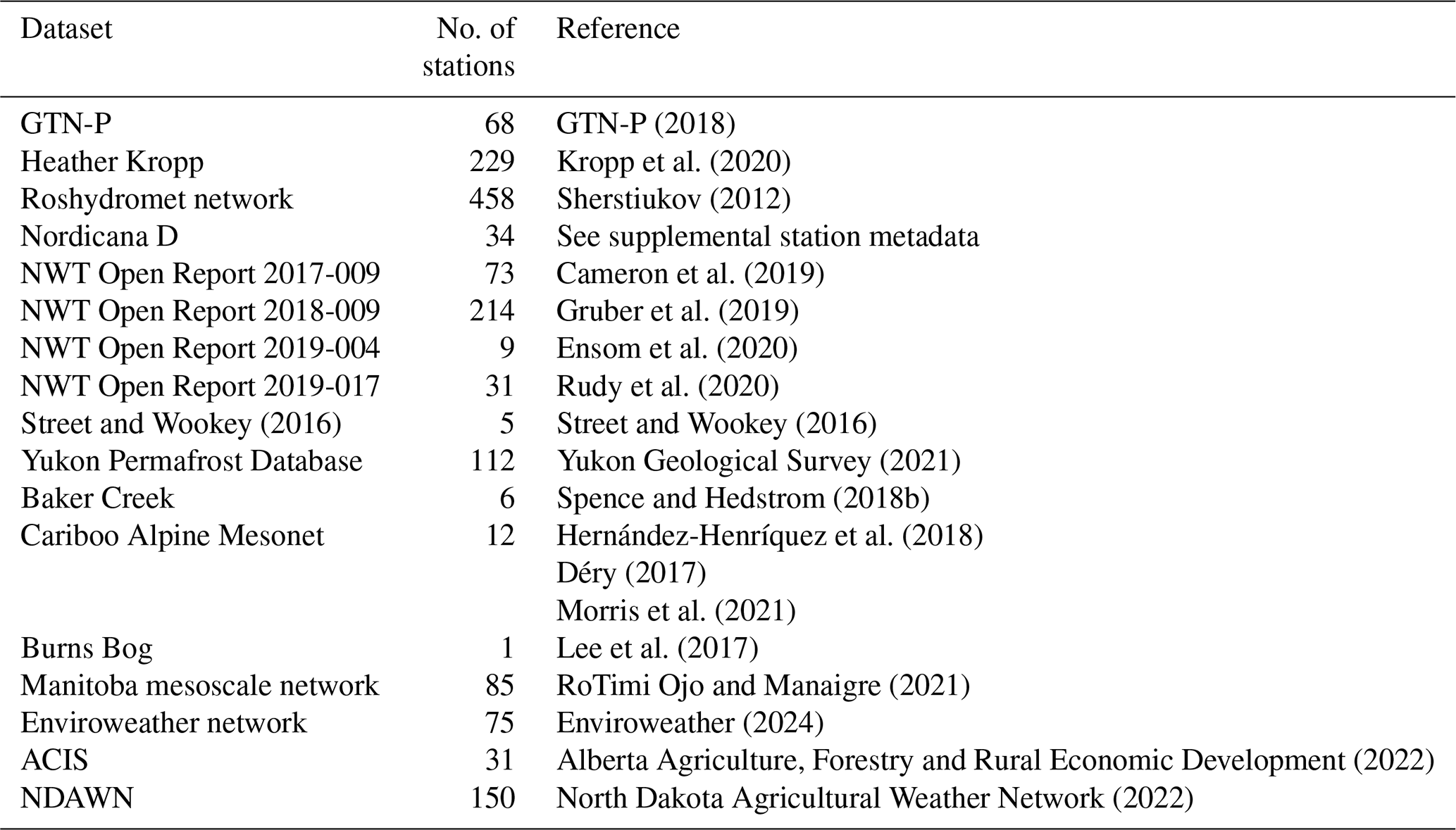
The study compiles a comprehensive set of in situ soil temperature measurements, approximately 1700 stations in total, from across extratropical Eurasia and North America (Table 3; also see the Supplement). Incorporating data from multiple diverse sparse networks, the dataset includes data from the Yukon Geological Survey (Yukon Geological Survey, 2021), the Northwest Territories (Cameron et al., 2019; Ensom et al., 2020; Gruber et al., 2019; Spence and Hedstrom, 2018a, b; Street et al., 2018), Roshydromet network in Russia (Sherstiukov, 2012), Nordicana series D (Nordicana) (Allard et al., 2020; CEN, 2020a, b, c, d, e, f, g), Global Terrestrial Network for Permafrost (GTN-P) (GTN-P, 2018), and Kropp et al. (2020) – in an attempt to provide a representative estimate of soil temperature across the circumpolar Arctic. Our validation data also include sites from outside regions typically underlain by permafrost in order to facilitate a comparison of the performance of reanalysis soil temperatures at high latitudes with their performance in regions outside the permafrost zone. These include stations from Kropp et al. (2020), Sherstiukov (2012), and GTN-P (2018), as well as locations from the Manitoba Mesonet network (RoTimi Ojo and Manaigre, 2021), the Michigan Enviroweather network (MAWN) (Enviroweather, 2024), the North Dakota Agricultural Weather Network (NDAWN) (North Dakota Agricultural Weather Network, 2022), and the Alberta Climate Information Service (ACIS) network (Alberta Agriculture, Forestry and Rural Economic Development, 2022). Data are also sourced from a peatland ecosystem in Metro Vancouver (British Columbia) (Lee et al., 2017), as well as several locations in central and northern British Columbia. (Déry, 2017; Hernández-Henríquez et al., 2018; Morris et al., 2021). This provides a unique baseline upon which to perform a hemispheric wide assessment of soil temperature in reanalysis and LDAS systems, and to the authors' knowledge, it presents the most comprehensive analysis to date of soil temperatures across Canada and the Great Lakes basin.

GTN-P (2018)Kropp et al. (2020)Sherstiukov (2012)Cameron et al. (2019)Gruber et al. (2019)Ensom et al. (2020)Rudy et al. (2020)Street and Wookey (2016)Yukon Geological Survey (2021)Spence and Hedstrom (2018b)Hernández-Henríquez et al. (2018)Déry (2017)Morris et al. (2021)Lee et al. (2017)RoTimi Ojo and Manaigre (2021)Enviroweather (2024)Alberta Agriculture, Forestry and Rural Economic Development (2022)North Dakota Agricultural Weather Network (2022)

Table 3 Summary of the observational data networks included in this study, with the dataset name, number of stations, and their references. Note that Nordicana D references are listed by site in the supplemental metadata.

2.3 Collocation of station and reanalysis data

In order to compare with data from reanalysis and LDAS products, temperatures were averaged across two depth bins: a near-surface layer (0–30 cm) and soil temperatures at depths ranging from 30 to 300 cm. For each site, temperatures from all depths residing within a layer were averaged, producing an estimated layer-averaged temperature for every time step. In order to maximize the amount of observational data available, layer-averaged soil temperatures were calculated at each time step with all available data. This tradeoff meant that layer averages often included a different number of depths at different time steps, and as such, we needed to limit our analysis of soil temperature trends and variability to locations where layer averages had a consistent number of depths.

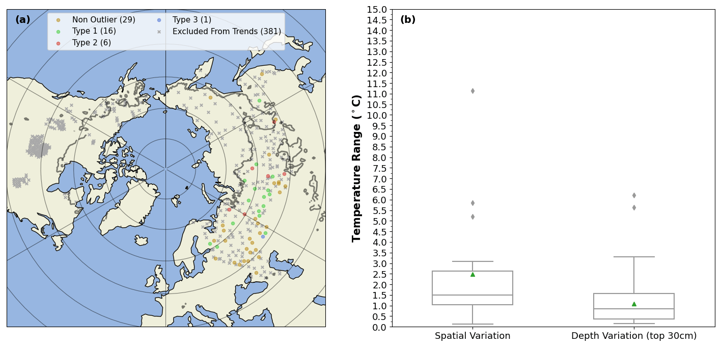
Figure 1 Panel (a) shows the location of the validation grid cells collocated with in situ stations in the near-surface layer. Grid cells excluded from the soil temperature trend analysis are shown as an “×”. Type 1 refers to grid cells where the ensemble mean simulates a winter minimum soil temperature that is too cold. Type 2 refers to grid cells where the ensemble mean simulates a summer maximum soil temperature that is too cold. Type 3 refers to grid cells where the ensemble mean underestimates the seasonal cycle of soil temperatures. The number in brackets beside each legend entry displays the number of grid cells in each category. The contour lines encircle regions where the Obu et al. (2018) permafrost cover is at least 50 %. Panel (b) shows the impact of spatial variation and depth variation on the spread of soil temperatures in a grid cell. The mean is shown by a green triangle and outliers are shown as grey diamonds.

Many of the in situ (station) sites reported measurements at hourly or daily frequency; however, we chose to perform the analysis at monthly time scales in order to focus on processes controlling the seasonal cycle of soil temperatures. As such, we use monthly averages of soil temperatures for validation purposes. Outlier observations with anomalies greater than ±3.5σ were removed before monthly averaging.

Since the station data often included days with missing observations, the sensitivity of the monthly averages to missing data was tested by computing monthly averages in five ways: using all months with at least 1 valid day in a month, using all months with at least 25 %, 50 %, and 75 % valid data, and finally, using all months with no missing data in a month. It was found that T_soil was not substantially impacted by the inclusion or exclusion of months containing missing data. In order to increase sample size, we therefore included all months with at least 50 % valid data.

In order to be considered as a validation location, the grid cell was required to include soil temperature data for all eight reanalysis/LDAS products and be collocated with at least one in situ station. Duplicate stations across datasets were excluded. In situ locations were only included if there was at least 2 years of in situ data in order to properly assess the station's seasonal cycle. For grid cells containing multiple in situ stations, the value used in the comparison is a simple spatial average of the in situ stations in that grid cell on each calendar day.

Over Eurasia, grid cells contained a single in situ measurement location. In North America, however, a number of the grid cells contain two or more in situ stations. The near-surface layer includes 430 validation grid cells (Fig. 1a), while at depth there are 377 grid cells (not shown). A subset of stations with longer time series and a more complete data record are used to calculate soil temperature trends (Sect. 4.2). Stations included in the soil temperature trend and variability analysis are shown as circles of varying size and colour, while those excluded from the soil temperature trend and variability analysis are shown as an “×” (Fig. 1a). The details of Fig. 1a will be described further in Sect. 5.3.

To calculate spatial averages, a simple average of (layer-averaged) soil temperatures from all stations within the bounds of a particular grid cell was calculated at each time step using all available stations. This meant that the number of stations included at each time step was not always consistent, and the analysis of soil temperature trends was limited to a subset of 52 grid cells in Eurasia where the following conditions were met:

1. The time series included data between January 1985 and December 2010, with no missing data.

2. The number of stations included in the spatially averaged grid cell temperature was consistent over all time steps.

3. The number of depths included in the layer-averaged soil temperature of each contributing station remained consistent over all time steps.

As a result, North American grid cells were excluded from the soil temperature trend analysis, and the analysis is based on grid cells from Eurasia (where grid cells often only contained a single station) (Fig. 1a). Using a subset of grid cells that incorporate multiple stations in the spatial average, and include a consistent number of stations and depths in the time series, we quantified the variability in soil temperatures between stations within a grid cell and across depths within a layer average. It was found that the median temperature range between stations within a grid cell was approximately 1.5 °C, roughly 1.75 times larger than the median temperature range across depths within the near-surface layer of a station (Fig. 1b), suggesting that temperature variability within a grid cell is substantially larger than variations in temperatures within the near-surface layer of a particular station.

3 Methods

3.1 Validation metrics

Reanalysis and observational (station) soil temperature data were collocated with one another spatially and temporally. Grid-cell-level soil temperatures from each product were compared against in situ soil temperatures using the following statistical metrics: bias (Eq. 1), root-mean-squared error (RMSE) (Eq. 2), normalized standard deviation (σ_norm) (Eqs. 3 and 4), and the Pearson correlation coefficient (R) (Eq. 5). We also include an overall skill score for each model, i.e., a Thackeray et al. (2015) type formulation of the Taylor (2001) skill score (SS) (Eq. 6). Statistical metrics were calculated as follows:

$$\begin{array}{}\text{(1)}& {\displaystyle }\mathrm{Bias}={\displaystyle \frac{\mathrm{1}}{N}}\sum _{n=\mathrm{1}}^N(T_{\mathrm{p}}-T_{\mathrm{i}})\text{(2)}& {\displaystyle }\mathrm{RMSE}=\sqrt{{\displaystyle \frac{\mathrm{1}}{N}}\sum _{n=\mathrm{1}}^N(T_{\mathrm{p}}-T_{\mathrm{i}}{)}^{\mathrm{2}}}\text{(3)}& {\displaystyle }\mathit{\sigma }=\sqrt{{\displaystyle \frac{{\sum }_{n=\mathrm{1}}^N(x_n-\stackrel{\mathrm{‾}}{x}{)}^{\mathrm{2}}}{N-\mathrm{1}}}}\text{(4)}& {\displaystyle }{\mathit{\sigma }}_{\mathrm{norm}}={\displaystyle \frac{{\mathit{\sigma }}_{T_{\mathrm{p}}}}{{\mathit{\sigma }}_{T_{\mathrm{i}}}}}\text{(5)}& {\displaystyle }R={\displaystyle \frac{\frac{\mathrm{1}}{N}{\sum }_{n=\mathrm{1}}^N(T_{\mathrm{p}}-\stackrel{\mathrm{‾}}{T_{\mathrm{p}}})(T_{\mathrm{i}}-\stackrel{\mathrm{‾}}{T_{\mathrm{i}}})}{{\mathit{\sigma }}_{T_{\mathrm{p}}}{\mathit{\sigma }}_{T_{\mathrm{i}}}}}\text{(6)}& {\displaystyle }\mathrm{SS}={\displaystyle \frac{\mathrm{2}(\mathrm{1}+R)}{{\left({\mathit{\sigma }}_{\mathrm{norm}}+\frac{\mathrm{1}}{{\mathit{\sigma }}_{\mathrm{norm}}}\right)}^{\mathrm{2}}}},\end{array}$$

where T_p is the T_soil from the reanalysis product and T_i is the T_soil of the in situ data. $\stackrel{\mathrm{‾}}{T_{\mathrm{p}}}$ and $\stackrel{\mathrm{‾}}{T_{\mathrm{i}}}$ refer to the mean T_soil of the reanalysis product and in situ data, respectively, and N is the number of monthly soil temperature values. ${\mathit{\sigma }}_{T_{\mathrm{p}}}$ and ${\mathit{\sigma }}_{T_{\mathrm{i}}}$ are the standard deviations of the reanalysis product soil temperatures and in situ soil temperatures, respectively. Finally, x refers to the T_soil (from a particular time step in a dataset) and $\stackrel{\mathrm{‾}}{x}$ is the mean T_soil of the dataset.

Metrics were calculated separately for each grid cell and then averaged to obtain regional values. Estimates for the permafrost zone and the zone with little to no permafrost were also calculated by averaging together metrics from grid cells falling within a particular zone. Skill scores were calculated separately for the near surface and depth, while the “overall” skill score represents an average of the near-surface and depth skill scores.

3.2 Binning of datasets by season and permafrost

Datasets were binned into a cold season and warm season using the University of East Anglia's Climatic Research Unit (CRU) TS version 4.07 2 m air temperature (T_air) (Harris et al., 2020) for each grid cell. Cold season months are those where $T_{\mathrm{air}}\le -\mathrm{2}$ °C, while the warm season refers to months with $T_{\mathrm{air}}>-\mathrm{2}$ °C, where T_air is the monthly mean air temperature. Sensitivity testing on the cold/warm season revealed no substantive impact on our conclusions using a threshold of 0, −5, and −10 °C. We also tested the impact of using a different temperature dataset to perform the binning: the ERA5 2 m air temperature, which resulted in similar findings.

Permafrost zonation was estimated using the Obu et al. (2018) permafrost map, which employs a temperature at the top of the permafrost (TTOP) model based on a 2000–2016 climatology, driven by a combination of remotely sensed land surface temperatures, downscaled atmospheric data from ERA-Interim, and land-cover information from The European Space Agency (ESA) Climate Change Initiative (CCI) (Obu et al., 2019). To maximize the sample size in each group, we merge the “continuous” and “discontinuous” permafrost zones into a single category called the “permafrost zone” and compare it against the zone with “little to no permafrost”, which includes all regions with <50 % permafrost cover.

3.3 Elevation impacts

The authors examined the potential impacts of elevation differences between in situ datasets and reanalysis products by estimating the station elevation using the 90 m Copernicus Global Digital Elevation Model (GLO-90) (European Space Agency, 2021) and obtaining reanalysis elevations at their native resolution for the nearest grid cell to the station. For grid cells with more than one station, station elevations were averaged together to obtain a grid cell estimate of the “station” elevation.

Grid cells were grouped into three elevation bins based on the station elevation, and it was found that over 70 % of grid cells are located in regions where the in situ station(s) are below 500 m (Table 4). Only 15 grid cells had station elevations above 1000 m, so the authors grouped all grid cells at or above 500 m together for the purposes of validation. While reanalysis products generally underestimated the elevation of higher elevation stations, with an average RMSE of between 144 and 589 m (not shown), this did not appear to have a major impact on soil temperature performance. (Readers are referred to Sect. 4.3 (“Spatial variability”) for more details.)

3.4 Regridding of reanalysis products and calculation of ensemble mean soil temperature

All products were first regridded to the ERA-Interim grid using a first-order conservative remapping technique (Jones, 1999). The near-surface soil layers, which are representative of the top 30 cm of soil, were calculated as a simple average of the top two soil layers in each reanalysis product. For JRA55, the single soil layer was used as a near-surface estimate. Soil temperatures at depth, for each product, were calculated as a simple average of all layers which fell between 30 and 300 cm, beginning with the third soil layer. For JRA55, the single averaged soil layer was used as an estimate of soil temperatures at depth. (Readers are referred to Table 2 for further information about product soil layers.) While the vertical discretization is coarser than that of the individual products, this approach allows the ensemble mean product to incorporate soil temperatures from products with different land models, whose vertical resolution is not constant.

Table 4 Number of grid cells in each elevation bin for the near surface and at depth.

After the near-surface and deep soil layer average temperatures were calculated for each product, the ensemble mean soil temperature, for each layer, was calculated as the unweighted arithmetic mean from six individual soil temperature products (CFSR, ERA-Interim, ERA5, ERA5-Land, FLDAS, and MERRA2). Owing to JRA55's simplified land model, which is unable to capture near-surface soil temperatures, we decided to exclude it from the ensemble mean product, as its inclusion dramatically increased the bias and RMSE of the ensemble mean.

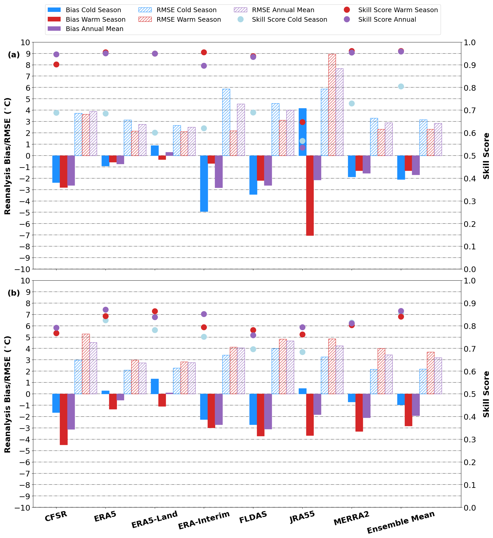
Figure 2 Bias (solid colour), RMSE (hatching), and skill scores (circles) of each product for the cold season (blue) ($\le -\mathrm{2}$ °C) and the warm season (red) ($>-\mathrm{2}$ °C) performance of reanalysis products. Bias, RMSE, and skill score over the annual mean are displayed in purple. Panel (a) displays the bias, RMSE, and skill score for the near-surface (0–30 cm) layer, while (b) displays the bias, RMSE, and skill score at depth (30–300 cm). The ensemble mean is shown beside for comparison.

4 Validation of reanalysis products

4.1 Annual mean

The Taylor skill score ranges between a minimum of zero and a theoretical maximum of one. A product with a skill score of 1.0 would display a perfect correlation of 1.0 relative to in situ soil temperatures and a soil temperature variance identical to that of the in situ data. Near the surface, most products display relatively high annual mean skill scores of > 0.9, suggesting that they generally capture the overall seasonal cycle of soil temperatures. At depth, skill scores are typically about 0.1 lower (Fig. 2; Tables S1 and S2 in the Supplement), arising from the lag between air temperatures and soil temperatures at depth. JRA55, however, displays an annual mean skill score of 0.54 near the surface and a skill score of 0.79 at depth (Fig. 2). This arises because JRA55 uses a simplified land model that uses just a single vertical layer, i.e., the soil temperatures used are computed as averages over the soil column and are, therefore, more similar to deeper soil layers than to the surface. Consequently, JRA55 underestimates the seasonal cycle of observed soil temperatures in the near surface, and the timing of its annual maximum and minimum soil temperatures is offset by roughly 1 month relative to other products (not shown).

Most products are biased cold over the annual mean and display soil temperature biases of between +0.3 and −3.1 °C, with RMSE values ranging between 2.5 and 7.7 °C over the extratropical Northern Hemisphere (Fig. 2; Tables S1 and S2). ERA5-Land is a notable exception as it shows a warm bias over the annual mean, driven by warm biases in winter, a factor that will be discussed further in Sects 4.2 and 6.1.

4.2 Seasonal cycle

As alluded to above, strong seasonal differences exist in reanalysis performance, with noticeably lower skill scores in the cold season. This is particularly true near the surface, where cold season skill scores are 0.08–0.35 lower than their warm season counterparts. Skill score declines at depth are reduced but still show a decline of 0.02–0.08 relative to the warm season (Fig. 2; Tables S1 and S2).

The decline in skill score is mirrored by increases in near-surface bias and RMSE for several products. This is particularly true for ERA-Interim, whose bias and RMSE are 4.1 and 3.7 °C larger, respectively. Interestingly, biases for all products are somewhat larger in the warm season at depth, though seasonal differences are also generally smaller in the deeper soil layers (Fig. 2). JRA55 and ERA5-Land are noticeable outliers to this trend, as they both exhibit positive (warm) biases in the cold season. In the case of JRA55, this is due to an underestimation of the seasonal cycle of temperatures, while for ERA5-Land, it is likely due to issues with snow cover properties (which will be discussed further in Sect. 6.1).

Near the surface, most products show a maximum cold (negative) bias when soil temperatures are between −2 and −10 °C, and there is a tendency for the biases of most products to decrease or flip sign over the coldest temperatures (Fig. 3), suggesting that they may underestimate the coldest in situ temperatures. At depth, however, most products display larger cold biases over warmer temperatures (Fig. 3b). JRA55 displays a maximum cold (negative) bias over the warmest temperatures and the bias flips sign as temperatures approach freezing, linked to its reduced seasonal cycle (Fig. 3). In the case of ERA-Interim, the largest cold (negative) biases are found over the coldest temperatures, likely linked to issues with its snow cover representation (discussed in Sect. 6.1).

Most products generally capture the observed soil temperature variance during the warm season. This is evident in Fig. 4b and d, as the normalized standard deviation is within 25 % of the observed variance for all products. This is contrasted by the cold season, where several products overestimate soil temperature variability (particularly at depth), contributing to a decline in product skill (Fig. 4a and c). For example, ERA5-Land's (blue diamond) cold season skill is impacted by its underestimation of cold season soil temperature variability (which is roughly half of the near-surface observed variance) and arises in part because of its warm (positive) bias in winter (Fig. 2).

The overestimation in soil temperature variance is also apparent in Fig. 5 as products display larger soil temperature variances (as measured by their standard deviation) for a given in situ soil temperature over colder temperatures. The spread in standard deviation between products (similar to their biases) is also generally largest over colder temperatures. The reduced standard deviation near the surface in the −32 °C bin is likely a function of the small sample size (11).

Similar seasonal variation is seen in reanalysis soil temperature correlations (against station data), as most products show warm season correlations of greater than 0.93 near the surface, with reductions of between 0.20 and 0.39 for most products over the cold season. At depth, warm season correlations are generally 0.09–0.18 lower than near the surface, and seasonal differences are much smaller (Fig. 4b and d). The poor JRA55 correlation near the surface arises from its mismatched seasonal cycle.

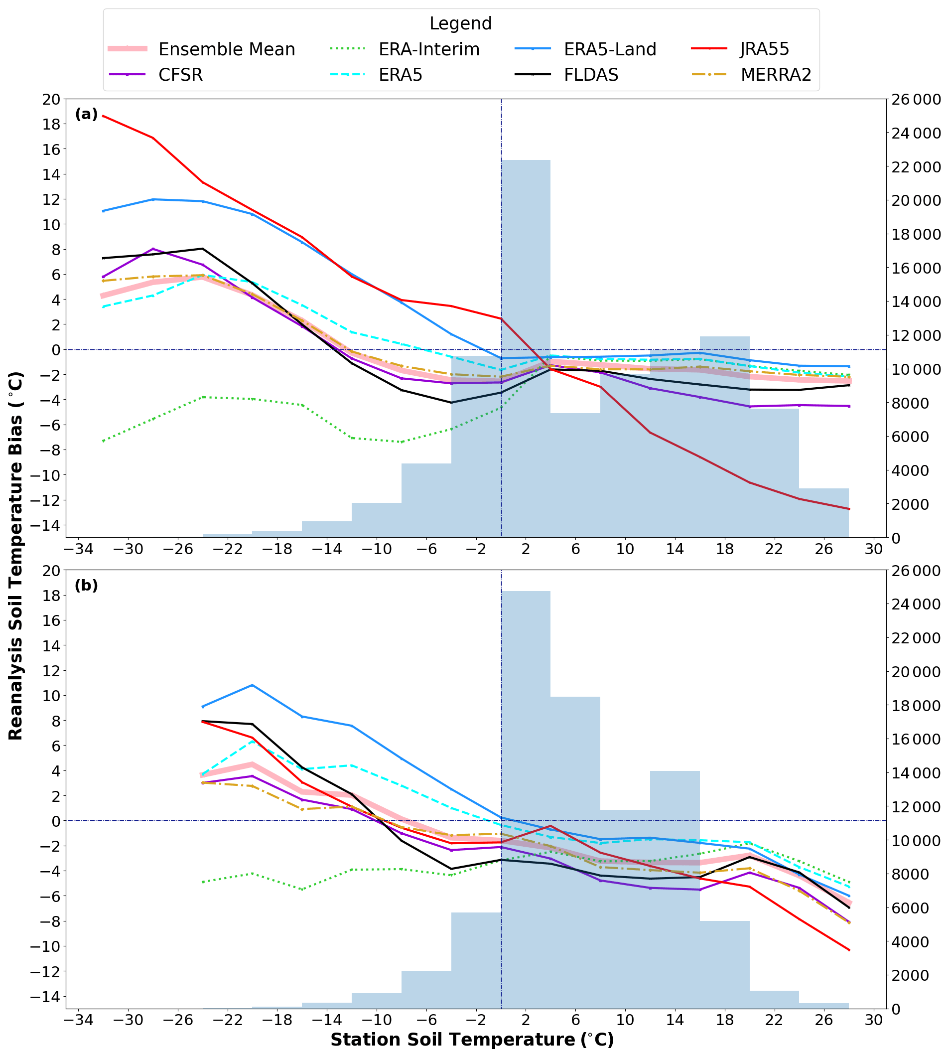
Figure 3 Reanalysis soil temperature bias as a function of station soil temperature for (a) the near-surface (0–30 cm) layer and (b) at depth (30–300 cm). Station temperatures are binned into 4 °C intervals, beginning with the −32 to −28 °C bin and ending with the 26–30 °C bin. The midpoint of each temperature bin is plotted along the x axis. The secondary y axis displays the number of data points in each bin (in conjunction with the histogram).

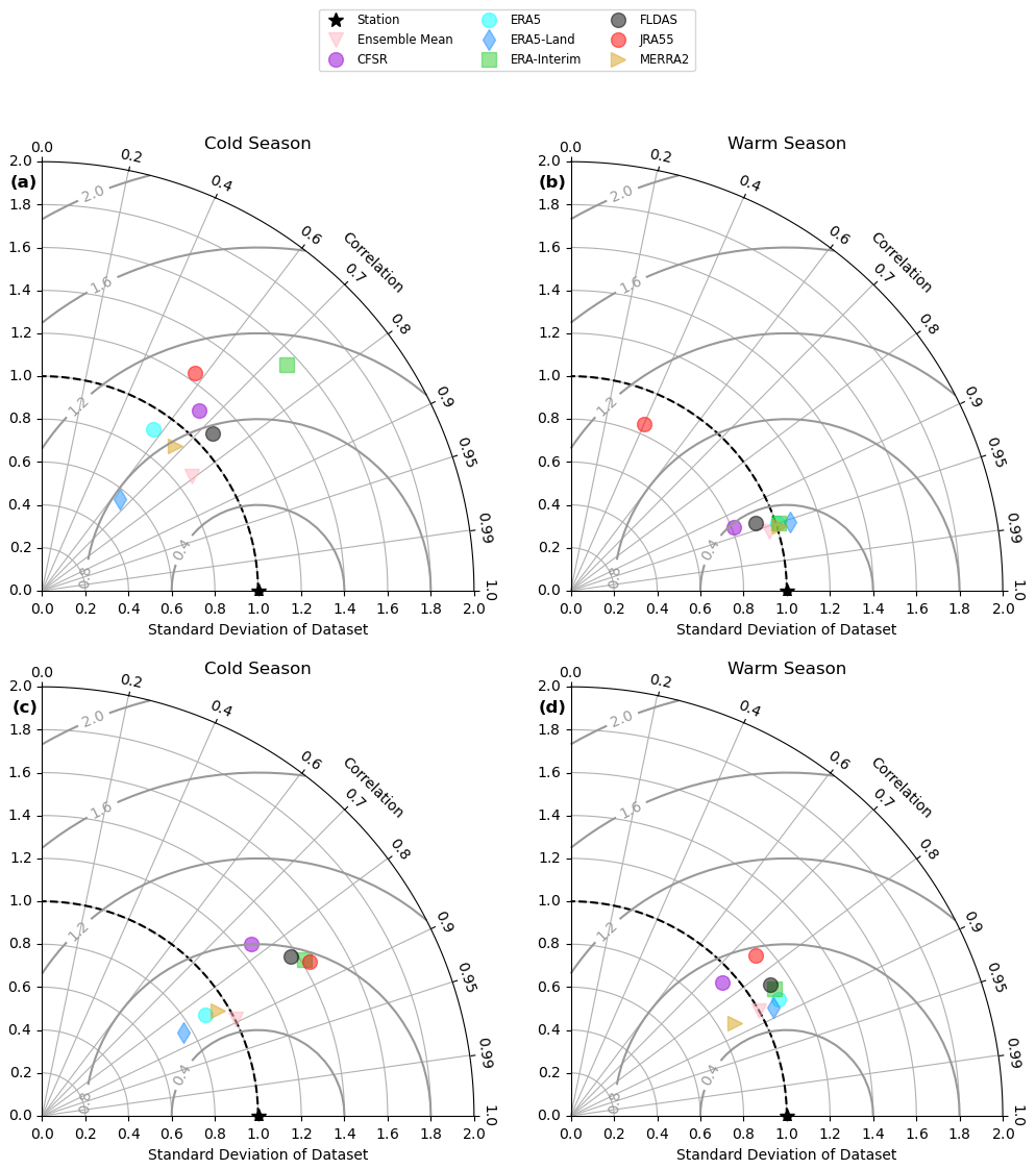
Figure 4 Taylor diagram of the cold season and the warm season performance of reanalysis products. Panels (a) and (c) refer to the cold season, while panels (b) and (d) refer to the warm season. The top panels, (a) and (b), are for the near surface, while the bottom panels, (c) and (d), refer to soil temperatures at depth. The concentric rings (solid grey lines) refer to the centralized root-mean-squared error (CRMSE), and a product would have a CRMSE of zero, with a normalized standard deviation of one and a correlation of one, if the time series of the reanalysis matched the station data perfectly.

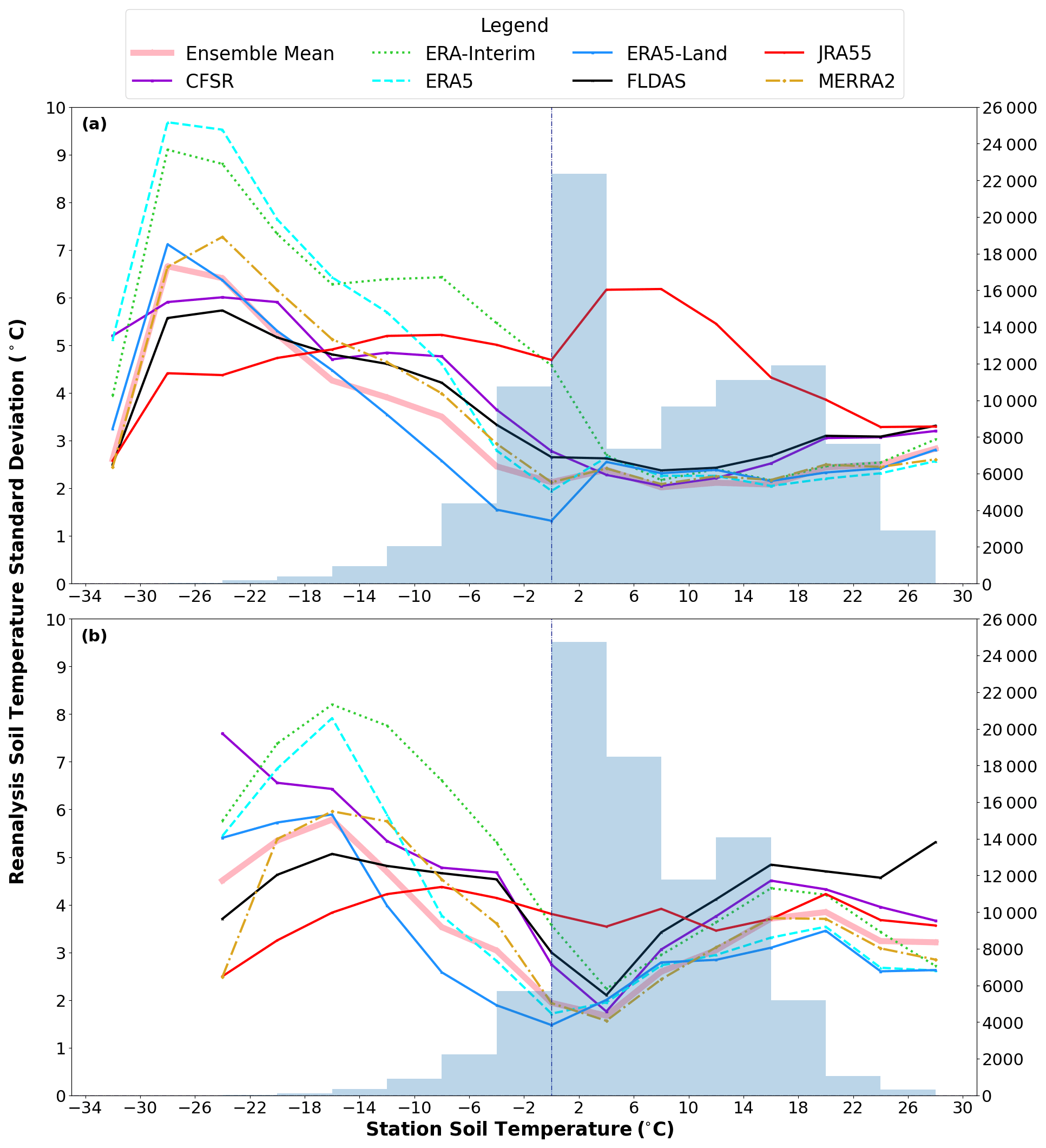
Figure 5 Reanalysis soil temperature standard deviation as a function of station soil temperature for (a) the near-surface (0–30 cm) layer and (b) at depth (30–300 cm). Station temperatures are binned into 4 °C intervals, beginning with the −32 to −28 °C bin and ending with the 26–30 °C bin. The midpoint of each temperature bin is plotted along the x axis. The secondary y axis displays the number of data points in each bin (in conjunction with the histogram).

4.3 Spatial variability

Similar to the strong seasonal differences in product performance, we also see substantial spatial variability in performance that is strongly linked to latitude. Over the permafrost regions, where snow cover lasts longer, soil temperature performance is typically worse than over regions further south. Near the surface, skill scores over permafrost regions are typically 0.05–0.1 lower over the annual mean than in regions with little to no permafrost, and at depth, they are generally between 0.07 and 0.26 lower (Fig. 6). The one exception is JRA55, which actually sees a slightly higher skill score over permafrost regions, driven by slight declines in RMSE over the cold season relative to regions further south. It remains for future studies to determine whether these differences are due to permafrost regions being colder or due to structural issues with the land models, as this is beyond the scope of this study.

Mirroring the lower skill scores in most products are larger RMSEs over the permafrost regions. This is particularly true during the cold season, when the RMSE for most products is typically 1.3–4.5 °C larger (Fig. 6) than over the zone with little to no permafrost. Warm season RMSE is also larger for most products in the permafrost zone, though by a lesser margin (0.1–2.1 °C).

Bias is also typically larger over permafrost regions by 0.63–3.9 °C. The ERA5-Land warm (positive) bias in the cold season is largest over permafrost regions (Fig. 6). In the case of JRA55, however, the warm (positive) biases over the cold season are largest further south. In fact, over many grid cells in the permafrost zone, JRA55 exhibits a cold (negative) bias during the cold season (not shown).

Reduced agreement between products is also apparent over permafrost regions, particularly at depth, where the spread in standard deviation between products is roughly 1.6–3.7 times larger over the permafrost zone (Fig. S1 in the Supplement), because of substantial differences in the variance of ERA5-Land, JRA55, and ERA-Interim. Interestingly, the differences in correlation and standard deviation between the permafrost zone and the zone with little to no permafrost, in the near-surface soil layers, are less dramatic (Fig. S2).

Generally, the skill is higher over Eurasia than over North America (Fig. 7). The lower skill in North America arises in part due to the underestimation of seasonal cycle over many grid cells in the Yukon and an overestimation of variability in cold season temperatures over much of the Great Lakes region (Fig. S3). CFSR and JRA55 are exceptions, however, as they greatly overestimate the cold season variability over much of western Eurasia (not shown) and consequently exhibit lower Eurasian skill scores. Soil temperature correlations (with in situ soil temperatures) are also lower by about 0.02–0.08 for most products in the warm season over North America, relative to Eurasia (not shown), which further contributes to reduced skill over North America.

As there are few stations above 1000 m, elevation does not have a substantial impact on product performance (Fig. 8). The slight improvement in near-surface cold season performance in CFSR at higher elevations can be linked to a slightly higher correlation, while in ERA-Interim, the slightly higher skill score is due to a slight improvement in cold season temperature variance (not shown). Skill scores and correlations at depth (not shown in Fig. 8) are lower by about 0.05–0.1 over higher elevation stations; however, the overall conclusions are not altered.

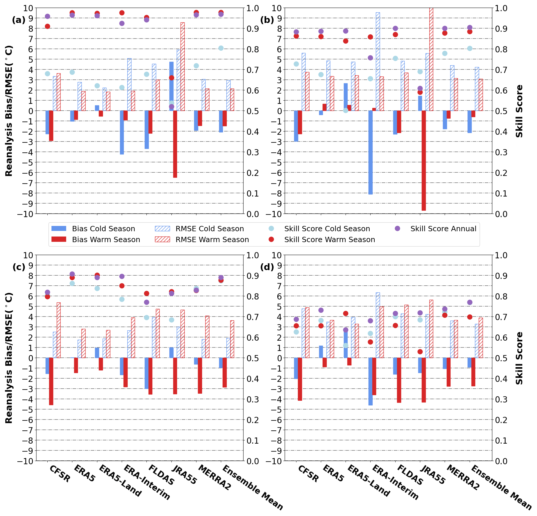
Figure 6 Bias (solid colours), RMSE (hatching), and skill scores (circles) of each product for the cold season (blue) and the warm season (red) performance of reanalysis products over the zone with little to no permafrost (a, c) and the permafrost zone (b, d). The skill score is also shown for the annual cycle (purple circles). Panels (a) and (b) display the bias, RMSE, and skill score for the near-surface layer, while (c) and (d) display the bias, RMSE, and skill score at depth. The ensemble mean is shown beside for comparison.

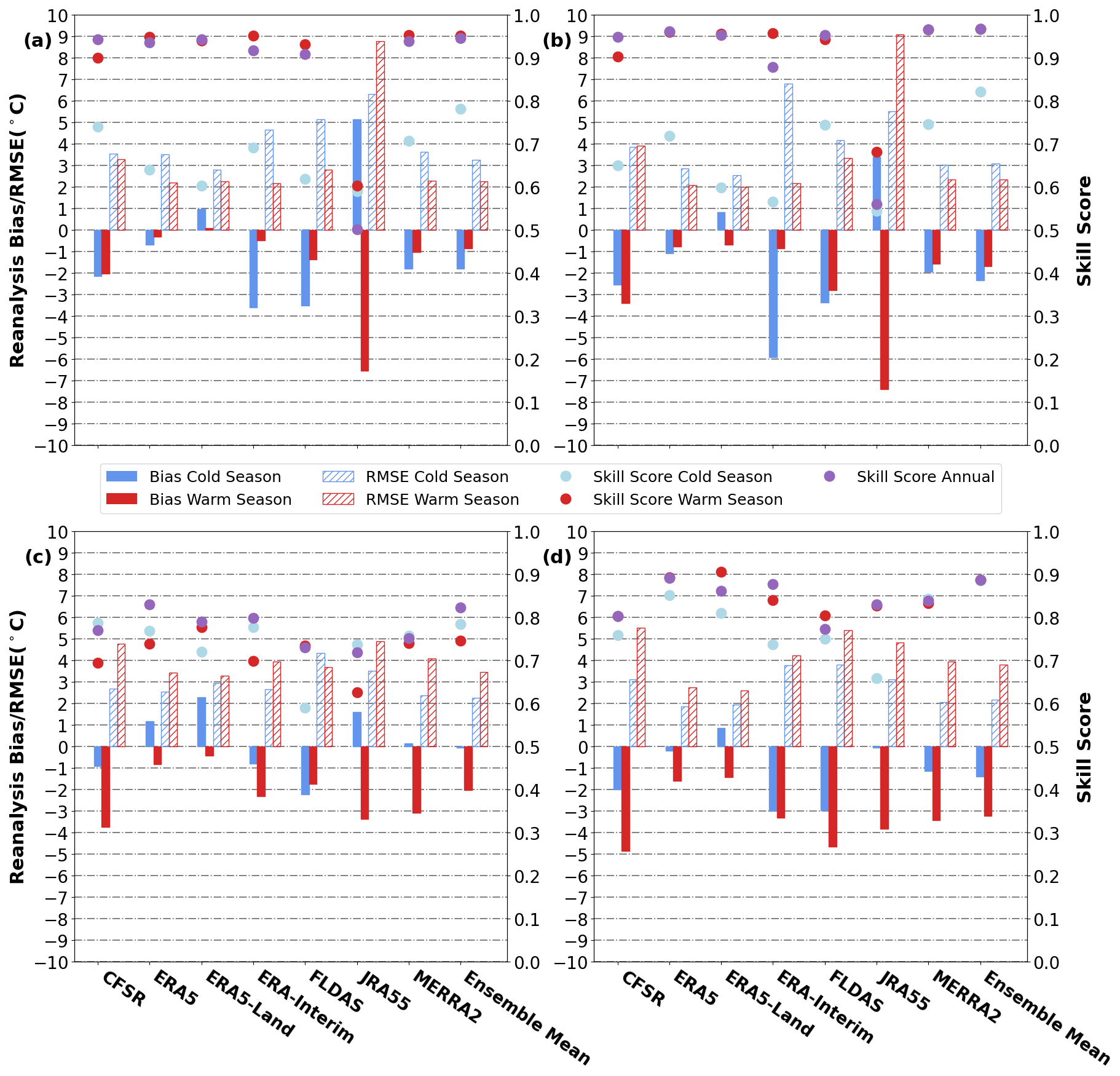
Figure 7 Bias (solid colours), RMSE (hatching), and skill scores (circles) of each product for the cold season (blue) and the warm season (red) performance of reanalysis products over North America (a, c) and Eurasia (b, d). The skill score is also shown for the annual cycle (purple circles). Panels (a) and (b) display the bias, RMSE, and skill score for the near-surface (0–30 cm) layer, while (c) and (d) display the bias, RMSE, and skill score at depth (30–300 cm). The ensemble mean is shown beside for comparison.

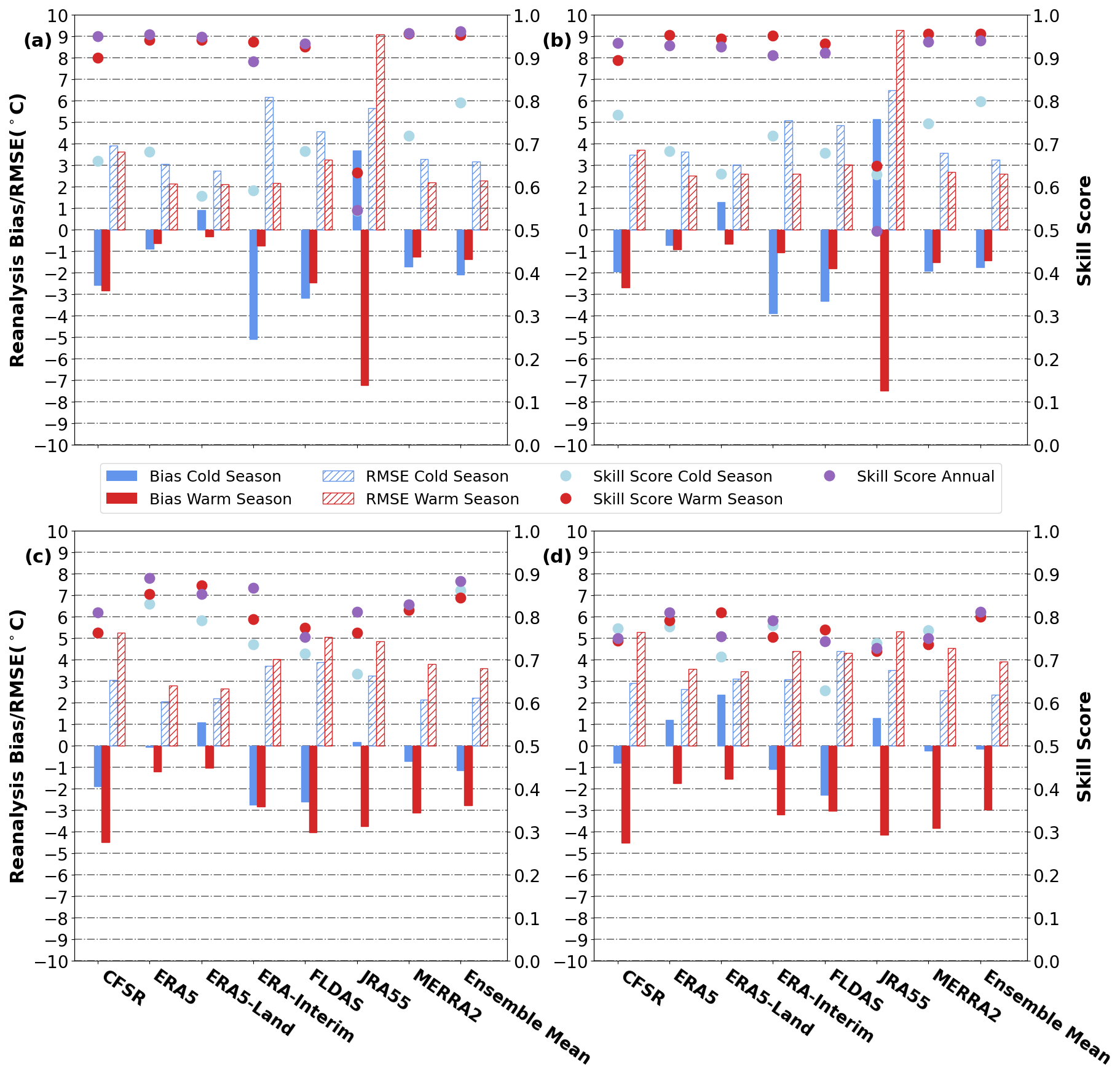
Figure 8 Bias (solid colour), RMSE (hatching) and skill scores (circles) of each product the cold season (blue) and the warm season (red) performance of reanalysis products over low elevation grid cells (below 500 m) (a, c), and grid cells at or above 500 m elevation (b, d). The skill score is also shown for the annual cycle (purple circles). (a) and (b) displays the bias, RMSE and skill score for the near-surface (0–30 cm) layer, while (c) and (d) display the bias, RMSE and skill score at depth (30–300 cm). The ensemble mean is shown beside for comparison.

4.4 Soil temperature trends

We calculate product trends over the 1985–2010 period in order to be able to calculate a station estimate from a subset of 52 Eurasian grid cells that have a continuous time series, as well as a consistent number of sites and depths included over all dates and times (denoted as the “Eurasian subset” hereafter). Trends at depth are very similar in magnitude and spatial pattern to the near surface, so we focus on the near-surface results here. Trends in the Eurasian subset (hatched bars in Fig. 9c) are generally representative of the Eurasian average (solid blue bars), though they are overestimated slightly in the case of CFSR.

Regionally averaged annual mean soil temperature trends show a small positive trend of < 0.5 °C  per decade in most products, over both Eurasia and North America, and trends in most products are generally consistent with the station estimate over the Eurasian subset (Fig. 9c). In CFSR (purple circles), however, the trend is near zero over North America and tends towards negative in Eurasia, arising because of anomalously cold years in 2009 and 2010 (see inset in Fig. 9a), and anomalously warm periods in the 1980s and early 1990s at the beginning of the time series (Fig. 9a and b). It is likely that the cold anomalies in 2009 and 2010 can be linked to issues with CFSR snow cover (Fig. S4, purple line) between January 2009 and January 2011.

Similar to skill score and RMSE, products show greater disagreement over higher latitudes (Fig. S5) and during winter (Fig. S6). ERA5 in particular, ERA5-Land, and to a lesser extent, ERA-Interim show several pockets of cooling over Siberia and the western Arctic over North America (Fig. S5), driven by strong cooling trends during December, January, and February (DJF) (Fig. S6). Meanwhile, the cooling trends in DJF are not as apparent in FLDAS, JRA55, and MERRA2. Trends over June, July, and August show good agreement between products, with most regions showing small warming trends of < 1 °C per decade and pockets of slight cooling over portions of Eurasia and western North America (Fig. S7).

Figure 9 Near-surface soil temperature anomalies and trends for each of the reanalysis products. Panel (a) displays the regionally averaged 1982–2018 annual mean soil temperature anomalies for each reanalysis product north of 40° N over Eurasia, while (b) displays the same but over North America. The CFSR time series is also shown as an inset to display the full range of values. Panel (c) exhibits an estimate of the regionally averaged 1985–2010 annual mean decadal soil temperature trend for each of the products and the ensemble mean for comparison. (The error bars represent the 95 % CI for the mean trend.)

4.5 Variability in seasonal extremes

The winter minimum and summer maximum show a cold bias over all latitude bands for most products (Fig. 10c and d), similar to the mean biases in the warm and cold seasons (Fig. 2). Similarly, the warm biases in ERA5-Land (blue diamond) and JRA55 (red circle) also extend to their winter maximum temperatures (Fig. 10c). The conclusions regarding variability in soil temperature extremes, at depth, are generally similar to those near the surface (Fig. S8c and d).

Table 5 Standard deviation (as a measure of spread between products) of the mean biases in winter minimum and summer maximum soil temperature, as a function of latitude and depth (from Figs. 10 and S8c and d). Latitude bands are 10° in width, such that the 40° N latitude band is an average between 40 and 50° N, while the 60° N latitude band is an average between 60 and 70° N, for example.

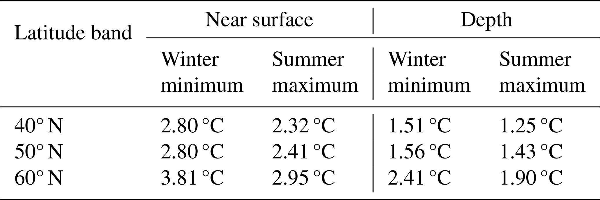
The spread between products in the bias of the summer maximum sees less latitudinal variation than the spread in the winter maximum over both depths, though the spread is largest near the surface (Table 5). Using the standard deviation as a measure of spread between product biases, the near-surface standard deviation in winter minimum bias increases from 2.80 °C over the 40° N latitude band to 3.81 °C north of 60° N (Table 5), in large part because of the large winter biases in ERA-Interim (Fig. 10c, green squares). Meanwhile, the spread in the summer maximum bias sees smaller increases (from 2.32 °C at 40° N to 2.95 °C at 60° N) (Table 5).

Figure 10 Performance of the near-surface soil temperature variability in the ensemble mean. Panel (a) is a scatterplot of the station and ensemble mean winter minimum soil temperature. Panel (b) is a scatterplot of the station and ensemble mean summer maximum soil temperature. Panel (c) shows latitudinal averages (from Eurasian grid cells) of the near-surface soil temperature winter minimum for the ensemble mean and contributing products. Panel (d) shows latitudinal averages (from Eurasian grid cells) of the near-surface soil temperature summer maximum for the ensemble mean and contributing products.

5 Ensemble mean product

5.1 Ensemble mean validation

The ensemble mean soil temperature product shows closer agreement with in situ soil temperatures than any of the individual products, when all depths, seasons, and regions are considered as a whole. First, its annual mean and cold season skill scores are higher than in any individual product. Second, its bias and RMSE are generally close in magnitude to the product with the lowest bias and RMSE over all depths and seasons (Fig. 2). Third, the ensemble mean product (Fig. 4, pink triangles) displays a temporal variance within 20 % of the observed variability over all depths and seasons, including in the cold season when many products fail to capture observed variance (Fig. 4).

The value of using the ensemble mean soil temperature is particularly noticeable in the cold season when individual products see a decline in skill, and a larger spread in performance. This is particularly noticeable in that its near-surface skill score in the cold season is nearly 10 % higher than the next best product (Fig. 2). Next, its correlation is roughly 0.05 larger than best individual product in cold season over both depths (Fig. 4). Moreover, its bias and RMSE only see relatively small increases over permafrost regions (Fig. 11), while products such as ERA5-Land, which have a small RMSE over more southern regions, see more substantial increases in bias and RMSE over the permafrost zone (Fig. S1). Thus, the ensemble mean soil temperature dataset provides the best estimate of in situ temperatures for the broadest range of conditions.

5.2 Ensemble mean soil temperature trends

We focus our analysis of trends on the near-surface data, as the spatial pattern of soil temperature trends near the surface and at depth show a pattern correlation of greater than 0.95 (not shown), and the conclusions regarding performance are generally similar. The ensemble mean shows a small positive soil temperature trend of 0.23 °C ± 0.09 °C per decade over Eurasia and 0.20 °C ± 0.109 °C per decade over North America between 1985 and 2010 (Fig. 9c). Most regions show small positive mean annual trends of < 0.5 °C per decade, though portions of North America and Siberia exhibit slight cooling trends of < 0.5 °C per decade (Fig. 12a).

Annual mean soil temperature trends in the ensemble mean over Eurasia show a strong correlation of 0.82 with observations (Fig. 12b). The ensemble mean also generally captures the correct sign of the observed trends, though it has a slight tendency to underestimate the magnitude of the trend (Fig. 12b). Trends at depth show a pattern correlation of 0.98 with the near surface (not shown in Fig. 12) and the conclusions are generally the same.

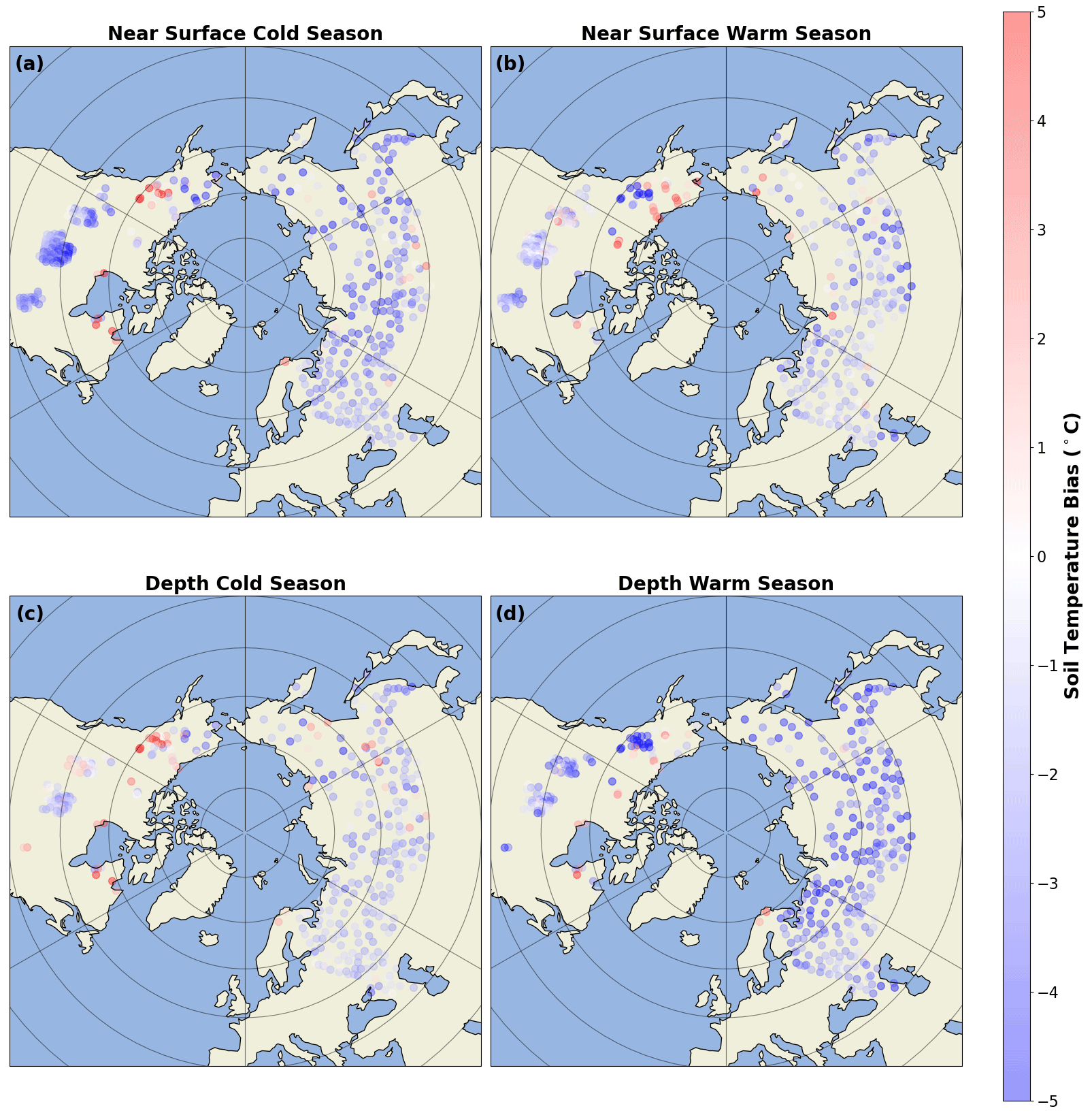
Figure 11 Spatial map of bias for the ensemble mean product. Values for the cold season are shown in the left-hand panels and those for the warm season are shown in the right-hand panels. Panels (a) and (b) show the near-surface bias, while biases at depth are shown in (c) and (d).

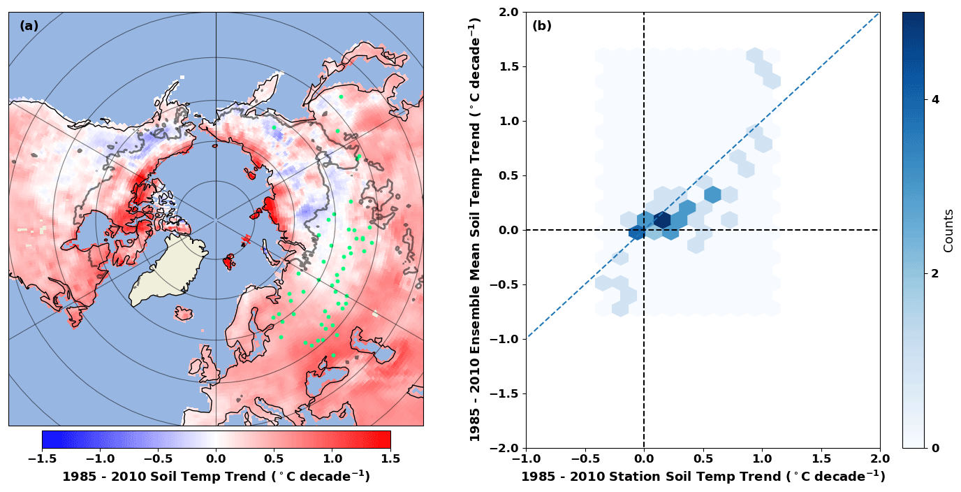
Figure 12 Panel (a) shows the 1985–2010 ensemble mean decadal soil temperature trends, near the surface, with the locations of validation grid cells included in the trend analysis shown as green dots. The grey contour line represents the boundary of the permafrost zone (regions with at least 50 % permafrost cover). Panel (b) shows the relationship between the near-surface ensemble mean and station soil temperature trends (per decade).

5.3 Ensemble mean variability in seasonal extremes

Similar to most products, the ensemble mean is biased cold in both the winter minimum (Fig. 10a) and the summer maximum (Fig. 10b) soil temperature. As Fig. 10a and b show, however, there is a fair degree of variability in the behaviour of the ensemble mean seasonal extremes – making an assessment of the mean behaviour in seasonal extremes somewhat tricky. Therefore, in the following paragraphs, we will focus on the most robust findings.

Near the surface, biases in the winter minimum soil temperature (Fig. 10a) are generally larger than in the summer maximum (Fig. 10b). This can also be seen in the latitudinally averaged soil temperatures, where the ensemble mean (pink line) is further from the station (black line) in the winter minimum (Fig. 10c) than in the summer maximum (Fig. 10d), which agrees with the findings that the near-surface cold season bias is generally larger than the bias in warm season (Fig. 2).

At depth, however, the summer maximum shows a larger bias (Fig. S8c) than the winter maximum (Fig. S8d), consistent with the finding that the extratropical mean bias is largest in the warm season at depth (Fig. 2). From Fig. S8b, we also see that the greatest disagreement in summer maximum occurs over the coldest regions.

Referring to Fig. 1a, several different types of grid cells are denoted. The first group, type-1 (16 occurrences) grid cells, is characterized by a strong cold bias in (underestimating) the winter minimum soil temperature (Fig. 13a). A second group of grid cells, which we refer to as type-2 (6 occurrences) grid cells, is defined as those which have a strong warm bias in (overestimating) the summer maximum temperature (Fig. 13b).

A common feature of the third group, type-3 grid cells, is that they underestimate the observed seasonal cycle of soil temperatures (Fig. 13c). While only one occurrence was found in the 52 Eurasian grid cells used for trend analysis, many grid cells in the Yukon would also show a similar underestimation of the seasonal cycle. This is evident as the ensemble mean normalized standard deviation (a measure of soil temperature variability) is substantially smaller than 1.0 in both seasons (Fig. S3). Often the in situ stations located within type-3 grid cells are located in areas devoid of vegetation, and it is likely that disagreements in the simulated vegetation cover in the contributing reanalysis products may partially account for the reduced seasonal cycle.

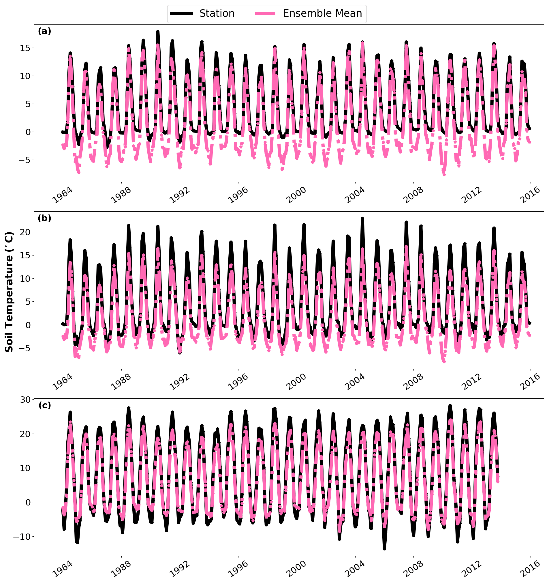
Figure 13 Time series from selected grid cells showing the ensemble mean (pink) and station (black) soil temperatures. Panel (a) displays a time series where the ensemble mean simulates a winter minimum that is too cold, (b) a time series where the ensemble mean simulates a summer maximum that is too cold, and (c) a time series where the ensemble mean underestimates the seasonal cycle of soil temperatures.

6 Discussion and conclusions

This study conducted a validation of pan-Arctic soil temperatures for eight reanalysis products and validated a new ensemble mean pan-Arctic soil temperature dataset. The results are qualitatively similar to the findings of previous studies exploring reanalysis soil temperature performance in the extratropical Northern Hemisphere, which generally highlighted a cold bias in most products (Hu et al., 2019; Qin et al., 2020; Wu et al., 2018; Xu et al., 2019; Yang and Zhang, 2018; Zhan et al., 2020). Similar to Li et al. (2021), we note greater biases in cold season soil temperatures, and our results qualitatively reflect the findings of Cao et al. (2020), who found that ERA5-Land exhibited warm soil temperature biases – particularly over higher latitudes.

The soil temperature trends reported here are of a similar magnitude to those reported by Biskaborn et al. (2019), who found that permafrost soil temperatures generally warmed at a rate of 0.29 °C ± 0.12 °C per decade, though ours differ in that they represent the mean extratropical Northern Hemisphere north of 40° N, whereas Biskaborn et al. (2019) predominantly focus on permafrost regions.

Other major differences here are that we developed an ensemble mean soil temperature product and had a greater focus on higher latitude regions than most other studies. We also note a strong difference in seasonal performance. Relative to the warm season, the cold season is generally characterized by lower skill, larger near-surface temperature biases, a larger spread in the reanalysis products' soil temperature variability, and lower correlations with in situ soil temperatures. When all depths and seasons are considered, the ensemble mean product performs better than any individual product, exhibiting a consistently high skill, realistic soil temperature variability, and relatively small biases over all seasons.

Here we show an approximate estimate of the magnitude of soil temperature uncertainty associated with instrumental uncertainties, and those associated with structural differences and parameterizations in land models, using the standard deviation in soil temperature across time and as a function of station temperature. A complete quantitative assessment of the contributions of various sources of uncertainty is not possible using this dataset, as time series did not have a consistent start or end date, and consequently, the metrics are calculated using different climatologies across different grid cells. A more complete uncertainty analysis is beyond the scope of this study but in the future could be achieved by limiting analysis to a subset of grid cells with consistent time series, for example, by focusing on soil temperature networks such as the Michigan Enviroweather network or the North Dakota Agricultural Weather Network, or limiting the uncertainty analysis to a smaller portion of the permafrost region.

We find that the median spread in the spatially averaged soil temperature of stations in a grid cell is approximately 1.49 °C (Fig. 1b) – several degrees smaller than the standard deviation of reanalysis soil temperatures for a given station soil temperature – particularly over frozen soils (Fig. 5). For example, when soil temperatures are below −20 °C, soil temperature standard deviations increase to near 10 °C in several products. Reanalysis 2 m air temperatures maintain a relatively consistent standard deviation between 1.25 and 1.75 °C for most products, and they only increase slightly to between 2.25 and 3.5 °C over the coldest station air temperatures (not shown). Unlike with soil temperatures, the spread in reanalysis 2 m air temperatures only increases modestly over the cold season (not shown). This would suggest that the largest degree of uncertainty in reanalysis soil temperatures over the Arctic is most likely caused by differences in the land models between products, rather than by uncertainties in observed soil temperatures, or from differences in product air temperatures.

6.1 Uncertainties associated with land model parameterizations and structural differences

Uncertainties in soil temperatures associated with structural differences and parameterizations in land models can be grouped into several categories. The first category surrounds the simplified parameterizations controlling frozen soil processes. For example, in the Noah LSM, utilized by CFSR and FLDAS, freeze–thaw processes are highly simplified and unsuited for permafrost simulations (Hu et al., 2019) – and may have contributed to the relatively large soil temperature biases simulated in these products. Even the best-performing products – ERA5 and ERA5-Land – are unsuited for simulation of permafrost soil temperatures, as they fail to simulate phase-dependent changes in soil thermal conductivity (Cao et al., 2020).

Yang et al. (2020) noted that larger soil temperature biases over the Qinghai–Tibetan Plateau in deeper soil layers were likely related to the fact that soil temperatures are less constrained by air temperature observations (and soil properties). This could also explain why soil temperature biases in the warm season are larger at depth than near the surface in this study. Moreover, the near-surface soil layers tend to fall within the active layer (which undergoes seasonal freeze–thaw cycles), while deeper soil layers are more likely to contain permafrost. Permafrost has a high degree of impermeability, which prevents soil water from infiltrating below the bottom of the active layer, and owing to latent heat considerations, leads to soil water freezing at the base of the active later (Zhao et al., 2000); however, these processes are not well represented in reanalysis LSMs (Yang et al., 2020; Hu et al., 2019).

LSMs, such as the Simple Biosphere Model (used in JRA55), that use the force restore method to estimate soil temperature are prone to overestimating diurnal soil temperature ranges (Gao et al., 2004; Kahan et al., 2006) as well as the seasonal cycle of soil temperatures (Luo et al., 2003). This is because they underestimate heat capacity and overestimate temporal variation in ground heat flux compared with more complex land models (Hong and Kim, 2010). Moreover, the force restore method assumes a strong diurnal forcing from above, an assumption that is likely violated when snow cover is present (Tilley and Lynch, 1998; Slater et al., 2001), because snow cover leads to a decoupling of the surface forcing from the soil below. These factors may help explain why JRA55 is unable to simulate near-surface soil temperatures as accurately as the other products explored in this study which explicitly incorporate representations of soil heat flux between soil layers (Niu et al., 2011; Koster et al., 2000; van den Hurk et al., 2000; Balsamo et al., 2009), and hence they are able to simulate a dampening of seasonal variability in soil temperatures at depth (and greater variability near the surface).

Burke et al. (2020) note that differences in snow cover properties were important in explaining soil temperature biases of several Coupled Model Intercomparison Project 6 (CMIP6) models, and it is likely that differences in snow cover properties between the LSMs studied here could account for some of the observed spread, particularly in the cases of ERA-Interim, ERA5, and ERA5-Land, because during the warm season, these products have similar soil temperature biases, but their performance varies widely during the cold season (Figs. 2 and 10), in large part because of snow density biases (Cao et al., 2020; Gao et al., 2022). In ERA-Interim, the large cold (negative) bias during the cold season is strongly related to the fact that it overestimates the observed snow density (Gao et al., 2022) and, consequently, also overestimates the thermal conductivity of the snow pack. Conversely, snow density (and thermal conductivity) in ERA5-Land (and ERA5) is too low, and hence biases in snow density are a large contributing factor to the warm (positive) bias during the cold season (Cao et al., 2020).

Snow was also cited as a major controlling factor in soil temperature biases in ECMWF's Integrated Forecast System, which also uses the HTESSEL land surface model (Albergel et al., 2015). In the case of the Noah LSM, which is included in CFSR/CFSv2 and FLDAS, Li et al. (2021) found that an overestimation of snow cover was a major contributor to larger soil temperature biases in winter over the Qinghai–Tibetan Plateau. Shukla et al. (2019) and Shukla and Huang (2020) found that overestimation of snow cover in CFSR during autumn and early winter leads to an overactive snow-albedo feedback and excessive cooling of the near-surface soil layers. This translates into a strong cold bias at depth over the spring and summer, and likely explains why CFSR's warm season bias and RMSE at depth are the largest of all seven products examined in this study (Fig. 2).

6.2 Uncertainties associated with scale effects

Here we evaluated soil temperatures at a relatively coarse resolution of 0.75°. As such, it is difficult for reanalysis products to capture local-scale variability in soil temperature. The subgrid-scale variability in soil temperatures calculated in Fig. 1b is of a similar magnitude to those calculated by previous studies exploring subgrid-scale variability in cryospheric soil temperatures (Gubler et al., 2011; Morse et al., 2012; Gisnås et al., 2014), though they are generally smaller than those reported by Cao et al. (2019). We found that the spatial variability in soil temperatures in one high latitude grid cell is larger than 10 °C at times (Fig. 1) – of a similar magnitude to those reported by Cao et al. (2019).

Moreover, as many grid cells in Eurasia only included a single in situ station, there is a significant chance that this single in situ station may not necessarily be reflective of conditions elsewhere in the grid cell (Gubler et al., 2011). When multiple in situ stations were available, we took the spatial mean of all stations in an attempt to estimate the mean soil temperature over the grid cell.

6.3 Uncertainties arising from sampling variability

As was described in Sect. 5.2, the presence of missing data created a challenge for calculating in situ soil temperature averages. While most grid cells in Eurasia had relatively consistent time series, and fewer issues with missing data, this was not the case over North America. Rather than limit our analysis to a small number of grid cells with little to no missing data (as we did for the calculation of soil temperature trends), we chose to make use of all available data at each time step when calculating our validation metrics (bias, RMSE, standard deviation, correlation, and skill score). Thus, the spatially averaged in situ soil temperature did not always contain a constant number of depths or grid cells at each time step in many grid cells over North America.

From Fig. 1b, it is apparent that the median variability in soil temperatures between stations within a grid cell (spatial variation), 1.49 °C, is roughly 1.75 times larger than the median variability in soil temperatures at different depths, 0.84 °C, for a particular station (depth variation). Thus, it would appear that fluctuations in the number of stations comprising the spatially averaged soil temperature are responsible for a greater proportion of the uncertainty than fluctuations in the number of depths included. However, it is also apparent that the uncertainties arising from variations in the number of grid cells included in a station average are substantially smaller than the spread between reanalysis products. During the cold season, the uncertainty in soil temperatures associated with the spread between reanalysis products is often two to three times larger than the uncertainty arising from fluctuations in station availability.

6.4 Applications and future work

The ensemble mean data product provides gridded, monthly-averaged soil temperature estimates of near-surface and deeper soil temperatures at a 0.75° resolution. Therefore, it is most suitable for regional or hemispheric-scale analyses of soil temperature climatologies, or their seasonal cycle, or to explore recent trends in soil temperatures. The product could also be used to provide boundary conditions for models that require soil temperature inputs, such as hydrological models, and for the validation of model soil temperatures. While the ensemble mean product still exhibits substantial cold biases over permafrost regions, and therefore is likely unsuitable for permafrost modelling, the RMSE over the permafrost zone of the ensemble mean product outperforms the RMSE of the best-performing product by 0.5 °C, on average (Fig. S1), in the cold season, and hence it may still provide some added value for estimation of high latitude soil temperatures relative to the individual products.

A robust ensemble mean can be computed with four products (not shown), which means a higher resolution ensemble mean data product could be created using a subset of the higher resolution reanalysis products. For example, ERA5, ERA5-Land, MERRA2, and CFSR have resolutions lower than 0.5°. Using a similar blending methodology, we have been investigating the performance of a 0.31° product (using a smaller subset of products that provide data at higher spatial resolution). We have also performed similar analyses with a 0.05° soil temperature product, using interpolated soil temperatures from the Arctic System Reanalysis version 2 (ASR), ERA5-Land, and FLDAS. The goal has been to assess the impact of spatial resolution on the performance of the ensemble mean product. We hope to include these results in a follow-up paper. Future work should aim to investigate how differences in snow cover and snow density between the reanalysis products may influence biases in the individual products. On a related note, future studies should also emphasize how differences in the land model structure and parameterization may account for the spread in soil temperatures.