Modelling present and future rock wall permafrost distribution in the Sisimiut mountain area, West Greenland

Degrading rock wall permafrost was found responsible for the increase in rockfall and landslide activity in several cold mountain regions across the globe. In Greenland, rock wall permafrost has so far received little attention from the scientific community, despite mountains being a predominant feature on the ice-free coastline and landslide activity being significant. In this study, we aim to make a first step towards a better understanding of rock wall permafrost in Greenland by modelling rock wall temperatures in the mountain area around the town of Sisimiut, which is 68° N on the west coast of Greenland. We first acquire rock surface temperature (RST) data for the period September 2020–September 2022 to model rock surface temperatures from weather forcing. The model is then applied to weather data from 1870 to 2022, generating rock surface temperatures to force transient heat transfer simulations over the same period. By extrapolating this method at the landscape scale, we obtain permafrost distribution maps and ad hoc simulations for complex topographies. Our model results are compared to temperature data from two lowland boreholes (100 m depth) and geophysical data describing frozen and unfrozen conditions across a mid-elevation mountain ridge. Finally, we use regional carbon pathway scenarios 2.6 and 8.5 to evaluate future evolution of rock wall temperatures until the end of the 21st century. Our data and simulation describe discontinuous permafrost distribution in rock walls up to roughly 400 m a.s.l. Future scenarios suggest a decline of deep frozen bodies up to 800 m a.s.l., i.e. the highest summits in the area. In summary, this study depicts a picture of warm permafrost in this area, highlighting its sensitivity to ongoing climate change.

1 Introduction

In cold mountain regions, complex topography influences shading, snow distribution, and ground type, causing a highly variable distribution of permafrost in steep rock walls (Etzelmüller, 2013). Several field studies describe a significant correlation between warming climate, rock wall permafrost degradation, and increased slope instability, observed as rockfall frequency (Ravanel and Deline, 2011; Gallach et al., 2020) and large rockslide occurrence (Patton et al., 2019; Guerin et al., 2020; Frauenfelder et al., 2018; Walter et al., 2020). Therefore, understanding the spatial distribution of rock wall permafrost and its future evolution is a key step in defining potential hazard areas (GAPHAZ, 2017), and several countries have started comprehensive programmes to monitor this phenomenon as a basis for risk assessment (Pellet and Noetzli, 2020; Isaksen et al., 2022).

In Greenland, the scientific community still does not have a precise quantification of rock wall permafrost distribution. Available models are based on kilometre-scale numerical simulations (Brown, 1960; Daanen et al., 2011), are not calibrated with in situ data (Gruber, 2012), or are valid only for sedimentary terrain (Obu et al., 2019). Furthermore, our understanding of the evolution of mountain permafrost in the region is limited, as only Daanen et al. (2011) investigate future permafrost distribution, although at 25 km resolution. This knowledge gap poses a significant challenge to our comprehension of mountain hazards and their evolution, hindering urgently needed regional-scale hazard assessment. This is particularly pressing due to the prevalence of landslides associated with permafrost degradation, as evidenced by prior studies (Svennevig, 2019; Svennevig et al., 2022, 2023; Walls et al., 2020), and the tangible impact of these events on the local population (Strzelecki and Jaskólski, 2020).

The fact that ground temperature data in Greenland are limited to a few lowland sedimentary boreholes that are not representative for rock wall bedrock permafrost in complex terrain is a major challenge for modelling this feature in this region. (Obu et al., 2019). A common strategy to overcome this issue is based on the approach developed in Switzerland in the early 2000s (Gruber et al., 2004) which involves the installation of multiple surface temperature loggers. These data are used for transient modelling of ground temperatures across 1D profiles in relation to depth (Westermann et al., 2016) and in 2D (Magnin et al., 2017) and more complex 3D geometries (Noetzli et al., 2007). Several studies model ground temperatures using numerical approaches, such as TEBAL (Stocker-Mittaz et al., 2002; Gruber et al., 2004) and CryoGrid (Myhra et al., 2017; Czekirda et al., 2023). Both models have a numerical approach to the evaluation of the surface energy balance (SEB), i.e. the transfer from weather parameters to surface energy flux as upper boundary conditions for the heat transfer module. Other studies have handled the SEB problem using an empirical approach based on correlating meteorological data and measured ground surface temperatures (Magnin et al., 2017; Etzelmüller et al., 2022; Rico et al., 2021; Legay et al., 2021). This approach has the advantage of obtaining good performances while requiring only basic climatic input, i.e. air temperature (AT) and solar radiation.

An additional source of data used to complement modelling efforts in the context of rock wall permafrost is offered by electrical resistivity tomography (ERT). ERT is a well-established method in rock wall permafrost research and investigations which has been demonstrated to provide information about the resistivity properties with high spatiotemporal resolution and can be interpreted in terms of the thermal state of subsurface materials (Hilbich et al., 2008; Keuschnig et al., 2017; Magnin et al., 2015b; Krautblatter et al., 2010; Scandroglio et al., 2021; Duvillard et al., 2021). ERT data can be acquired in complex terrain and gather relevant information in a relatively short time (Magnin et al., 2015b). The ERT data allow us to interpret the bedrock conditions as frozen/unfrozen and can be compared to the numerical simulations of ground temperatures, providing an additional source of model testing (Duvillard et al., 2021). In particular, this methodology provides a model of ground freezing conditions at a given survey date, which can validate numerical simulations (Magnin et al., 2017; Etzelmüller et al., 2022).

The aim of this study is to take the first step towards understanding the distribution patterns and future evolution of rock wall permafrost in Greenland. To reach our objective, we focus on the Sisimiut area (68° N on the west coast). In autumn 2020, we installed nine ground surface temperature loggers in the area measuring rock surface temperature (RST), covering the local range of elevations and aspects. Using these data, we train a statistical model to evaluate the correlation between weather variables (i.e. air temperature and incoming shortwave solar radiation) and measured RST. The statistical model is then used to generate the boundary conditions for a heat transfer model. We calibrate and test our model with temperature data obtained from two boreholes, each drilled to a depth of 100 m in lowland flat bedrock. The model is then used to generate rock wall temperatures at high elevation, which we compare to ERT data acquired in the field. These efforts aim to answer three research questions:

1. What is the current distribution of rock wall permafrost at our study site?

2. Can our model reproduce permafrost patterns in agreement with our dataset?

3. What is the possible evolution of rock wall permafrost by the end of the 21st century under different climatic projections?

2 Study site

Our study site is located in the mountains surrounding Sisimiut, a city on the coastline of the widest non-glaciated area in West Greenland, about 160 km from the Greenland ice sheet (see Fig. 1). Sisimiut is the second-largest city in Greenland, counting 5582 inhabitants in 2020 and experiencing a rapid development. The city is surrounded by two main mountain ridges: the Nasaasaaq–Appillorsuaq ridge to the south, summiting at 784 m a.s.l., and the Palasip Qaqqaa–Sammisoq ridge to the north, summiting at 605 m a.s.l. (see Fig. 1a). The landscape is characterized by narrow fjords, alpine summits, and isolated coastal glaciers. The dominant lithology is amphibolitic gneiss (Kalsbeek et al., 1987). The mountains of the region typically have pyramid-shaped summits and steep rock walls generating debris slopes underneath. The mountains are dominated by bedrock, although vegetation patches are common at up to 400 m a.s.l.

Sisimiut, located in the low Arctic oceanic area, is subject to climate data collected at the airport weather station (AWS) (Cappelen et al., 2021; Cappelen and Jensen, 2021) (see Fig. 1b). July, with an average temperature of 6.3 °C, marks the warmest month, while March is the coldest at −14.0 °C. These climatic characteristics classify Sisimiut within the sporadic permafrost zone (Obu et al., 2019; Biskaborn et al., 2019), and morphologically active rock glaciers extend to sea level elevation (see Fig. 1a).

The climate has undergone significant changes over the years. The mean annual air temperature (AT) increased from −3.5 °C during 1961–1981 to −1.8 °C in the period from 2000–2020. This shift in climate is also reflected in precipitation patterns. Mean annual precipitation decreased from 509 mm in 1961–1981 to 422 mm in 1984–2004, which coincides with the year the rain gauge was decommissioned. The reduction in precipitation affects both solid and liquid forms. For solid precipitation, mean monthly levels in January–April decreased from 28 mm in 1961–1981 to 25 mm in 1984–2004. Meanwhile, liquid precipitation, observed from June to September, dropped from 58 mm in 1961–1981 to 49 mm in 1984–2004. Recent climate change is believed to be responsible for significant glacial retreat along the coast. Coastal glaciers in the area have lost approximately one-quarter of their volume over the past 3 decades (Marcer et al., 2017).

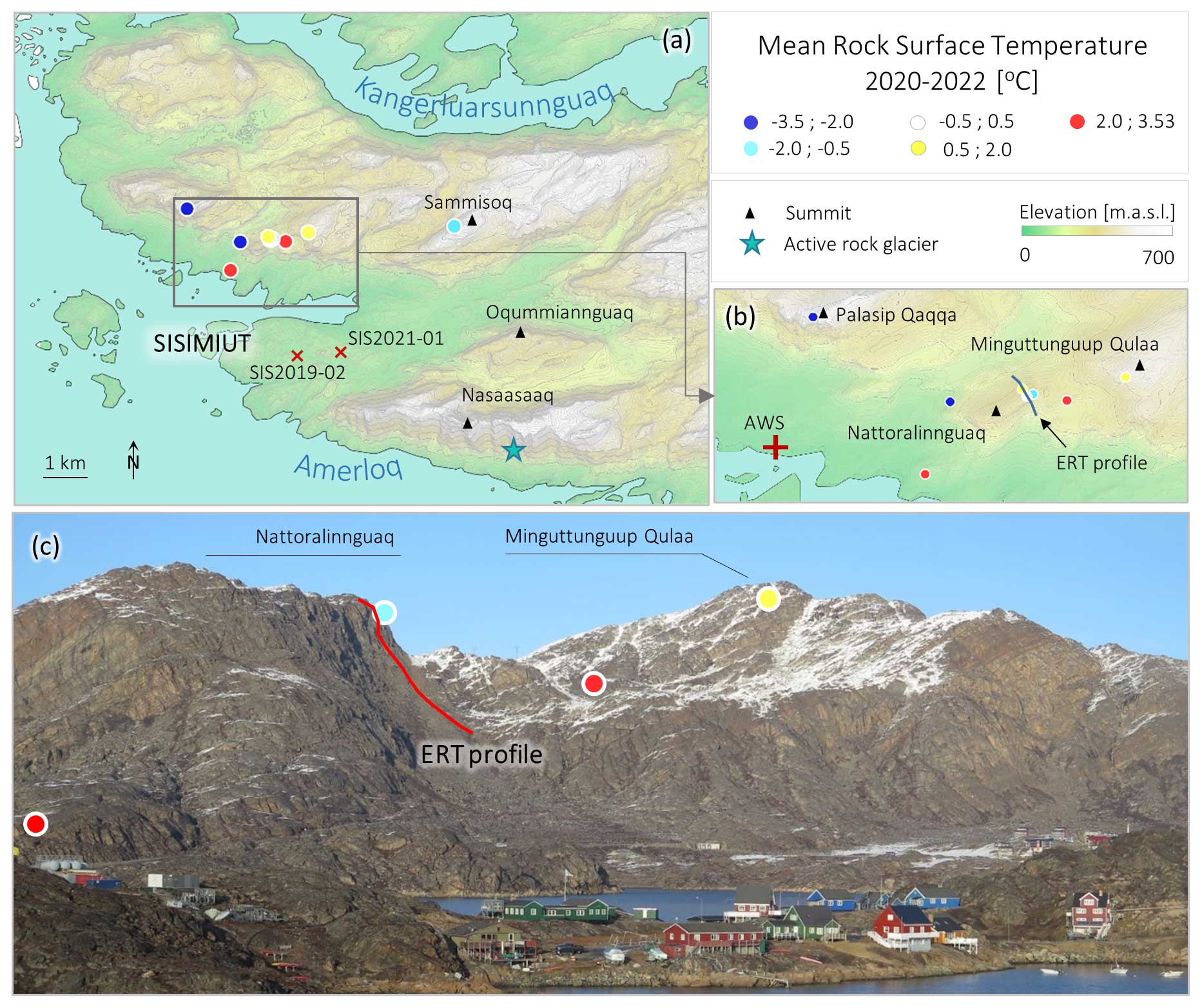
Figure 1 Study site summary. Map of the study area (a), with location of deep boreholes SIS2019-02 and SIS2021-01, main summits, and the active rock glacier. (b) Detail of the Nattoralinnguaq area, where most of the RST sensors are installed. (c) South face of Nattoralinnguaq and Miguttunguup Qulaa (picture taken from Sisimiut in October 2020) with RST loggers and geophysical profile locations. Loggers are coloured based on their measured mean RST acquired during the acquisition period (autumn 2020 to autumn 2022). Elevation data belong to the Arctic digital elevation model (Porter et al., 2018).

3 Methods

3.1 Rock wall temperature monitoring

Rock wall temperatures are measured by a network of temperature sensors installed in various settings across the study area. All sensors used for the temperature data acquisition were zero-point calibrated to custom using a Fluke 7320 compact bath with manufacturer-specified temperature stability and uniformity accurate to 0.01 °C. The bath temperature was measured using a Fluke 5610 Secondary Reference thermistor probe, and each sensor was immersed in the bath for 40 min while logging every 30 s. After the sensor temperature stabilized, the sensor offset was calculated as $\mathrm{\Delta }T=\left({\sum }_{(i=\mathrm{1})}^n\right[T_{\mathrm{ref},i}-T_{s,i}\left]\right)/n$, where T_s,i [°C] is the ith sensor temperature measurement in the calibration period; T_ref,i [°C] is the corresponding bath temperature measured by the Reference thermistor probe at the same time; and ΔT [°C] is the average calculated sensor offset, which was applied as a correction to each field temperature measurement collected by that sensor.

We established an RST monitoring network consisting of nine individual monitoring locations, covering as evenly as possible the range of aspects and elevations of the rock walls at the study site (see Fig. 1a). Data were acquired for 2 years, from autumn 2020 to autumn 2022. The technical information about loggers used is summarized in Table 1. GeoPrecision sensors are widely used in permafrost studies, and the community has previous experience in their strengths and weaknesses (Gruber et al., 2004; Magnin et al., 2015a, 2019; Hipp et al., 2014; Duvillard et al., 2021). According to our calibration, GeoPrecision offsets reach a maximum of 0.10 °C. GeoPrecision loggers can be accessed remotely, allowing download of data within a 10–20 m range, which becomes handy in steep terrain. The sensors were placed in 10×300 mm holes, thereafter sealed with frost-resistant resin.

Table 1 Summary of the temperature sensors and their specifications used in the study area.

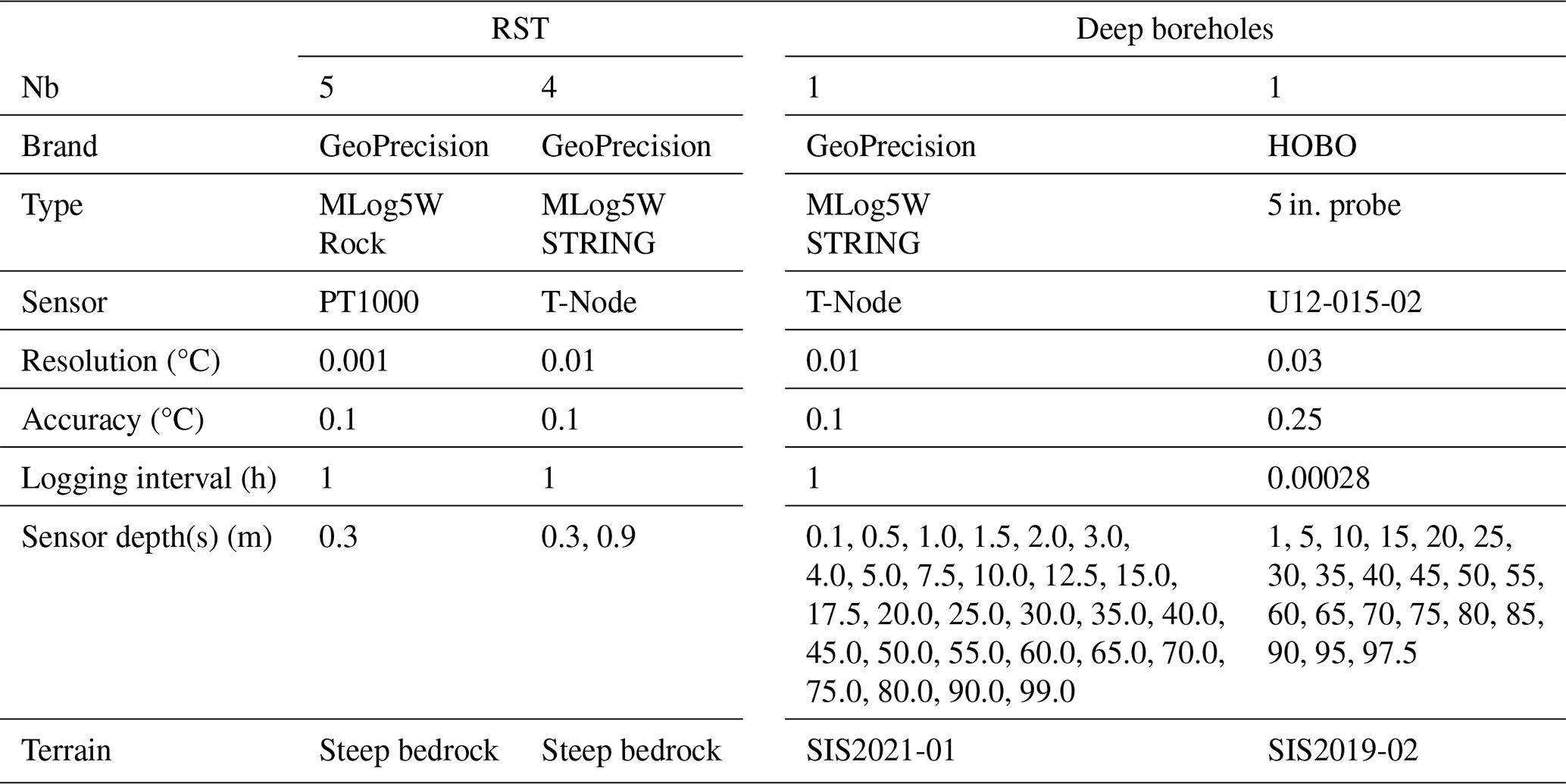
While deep boreholes in rock walls are not available in our study area, we have valuable data from two 100 m deep boreholes, SIS2019-02 and SIS2021-01, which were drilled into bedrock outcrops on flat terrain at 50 and 70 m a.s.l. within the town’s urban area (see Fig. 1a). While these locations differ from our primary focus on rock wall permafrost, we have incorporated their data into this study and will address the associated limitations in our discussion. The boreholes are located in similar conditions regarding the exposure to solar radiation, yet different snow conditions. SIS2019-02 is located in a drift accumulation area, and the snow depth can reach 2 m, while SIS2021-01 is on a wind-exposed hill, which ensures snow-free conditions for most of the winter. Both boreholes are drilled using a Sandvik DE130 compact core drill owned and operated by the Greenland School of Minerals and Petroleum, with wireline NQ drilling tools (outer diameter 70 mm). The holes are installed with a 100 m long PE casing (outer diameter 32 mm, inner diameter 26 mm), closed at the bottom with a heavy-duty heat shrink end cap with heat-activated glue.

Borehole SIS2019-02 does not have a permanent sensor installed, and the available dataset consists of four temperature profiles logged manually. This was done on three distinct dates: 27 October 2020, 17 November 2020, 20 January 2021, and 9 November 2021. For each measure we use a HOBO U12-015-02, logging at a 10 s sampling interval and resting at predefined depths for 2 min (see Table 1 for measuring depths). In the post-processing, temperatures are averaged only over the last minute to obtain the temperature at a particular depth, thereby ensuring the sensor has equilibrated to the new temperature. The borehole SIS2021-01 is equipped with a permanent GeoPrecision thermistor string with 28 sensors (T-Node, digital chip with 0.01 °C resolution). The uppermost sensor is located at 0.1 m below ground surface (m b.g.s.) and the lowermost at 99 m b.g.s. The sensor spacing progressively increases in depth from 0.4 m at the top to 10.0 m at depth, and the logging interval is 1 h.

3.2 Geophysical data

To obtain information on deep permafrost distribution in mountain terrain, we use the approach proposed by Duvillard et al. (2021), consisting of a combination of an ERT survey in the field and laboratory experience to calibrate the temperature–resistivity relationship characteristic of the rock. We conducted the ERT survey in October 2020, across the north and south faces of Nattoralinnguaq (353 m a.s.l.) (see Fig. 1b). This summit presents typical characteristics of the mountains in the Palasip Qaqqaa–Sammisoq ridge: a steep and rocky south face approximately 100 m high with a debris slope underneath and a more gentle north face characterized by small vegetation patches and some short, steeper sections (see Fig. 1c).

The ERT measure consists of one 450 m long profile (five 100 m long cables and a total of 100 electrodes deployed with 5 m spacing). We use a 12 V external battery for powering the resistivity meter (Guideline Geo Terrameter LS2) and injecting the current. We use 10 mm ×100 mm stainless-steel electrodes inserted into predrilled holes with a paste of salty bentonite to improve the galvanic contact and reduce the contact resistances and prevent freezing (Krautblatter and Hauck, 2007; Magnin et al., 2015b). For the data collection, we use the Wenner configuration. This configuration corresponds to having the voltage electrodes M and N in between the current electrodes A and B, with equal spacing between the electrodes. This array is characterized by an excellent signal-to-noise ratio (Dahlin and Zhou, 2004; Kneisel, 2006). Topography was extracted from a 2 m resolution digital elevation model (DEM; Porter et al., 2018) based on electrode positions measured with a handheld GPS device. We cleaned 4 % of the measures acquired before the inversion (549 measures acquired, 528 inverted) by filtering out the outliers and the data characterized by high standard deviations (higher than 10 %) from the pseudosection and the apparent negative resistivity. The data were inverted with RES2DINV 4.8.10 software using a smoothness-constrained least-squares method and the standard Gauss–Newton method (Loke and Barker, 1996). The inversion was stopped when the convergence criterion was reached. In this study, the convergence criterion is met when the change in the root-mean-square error (RMSE) between two iterations is below 10 % (default criterion in RES2DINV). In the present case, convergence is reached during the third iteration.

In addition to the field measurements, we perform a laboratory electrical conductivity experiment on three rock samples following the procedure described by Coperey et al. (2019). These analyses define the relationship between resistivity collected in the field and rock temperature under the assumption that the material is not fractured and isotropic. The rock samples are collected from the rock walls on the south and north faces (samples G-RF, G-LR, and G-DA) and are characterized by a porosity of Φ=0.032 for G-RF, Φ=0.015 for G-LR, and Φ=0.023 for G-DA. Before performing the laboratory measurements, each sample is cut in a $\mathrm{4}\times \mathrm{4}\times \mathrm{4}$ cm cube, dried for 24 h at 60 °C, and eventually saturated in a vacuum with degassed water from melted snow taken in the field. The cubes are then left several weeks in the solution to reach chemical equilibrium. The water conductivity at 25 °C and at equilibrium is 0.0118 Sm⁻¹ for G-DA and 0.0142 Sm⁻¹ for G-RF and G-LR. The cubes are then placed in a heat-resistant insulating bag immersed in a thermostat bath (KISS K6 from Huber; bath volume: 4.5 L). The bath temperature is regulated using an internal sensor with a precision of 0.1 °C, while the rock temperature is monitored with an additional sensor, also offering a precision of 0.1 °C. Glycol is used as a heat-carrying fluid, and the conductivity measurements are carried out with an impedance meter. The glycol is progressively cooled from 20 to −13 °C, stopping for 2.5 h at predefined temperatures to let the rock reach thermal equilibrium with the glycol (see Fig. 3b for sample-specific temperature steps). After the equilibrium is reached, the resistivity is measured.

3.3 Rock temperature modelling

Our modelling approach is based on a mixed statistical–numerical methodology, which is conceptually similar to the study developed by Magnin et al. (2017). The methodology evaluates RST time series with an empirical approach, and these are then used as upper boundary conditions for a heat transfer numerical model. This modelling methodology refers to a four-step workflow: (i) acquisition of weather forcing data and downscaling, (ii) statistical modelling and prediction of RST data, (iii) numerical modelling of heat transfer in bedrock, and (iv) model validation with field data.

3.3.1 Weather data and downscaling

The weather data are retrieved from different sources covering different periods, as summarized in Table 2. Our time domain is divided into three periods: (i) the historical period from 1870 to 1969, (ii) the current period from 1970 to 2022, and (iii) the future scenarios from 2023 to 2100. While a weather station at the Sisimiut airport has been recording AT since 1961 (Cappelen and Jensen, 2021) (dataset d in Table 2), it is noteworthy that such long-term data collection is rare in most areas in Greenland. Consequently, we have chosen to utilize weather data available at the regional scale to force our model and keep the Sisimiut weather station data as a validation set. This choice allows us to understand the modelling uncertainties inherent in regional-scale weather data, with the broader aim to assess how this methodology could perform if applied in other areas of the country. Therefore, we evaluate the performance of each of the following datasets by comparing their AT to the data from the Sisimiut weather station over the overlapping period.

The weather data for the current period are obtained from the ERA5 reanalysis, which we downloaded from the Copernicus database (Hersbach et al., 2020) (dataset b in Table 2). For this study, we use the AT at pressure levels from 1000 to 500 hPa and shortwave solar radiation downwards (SSRD) at the surface level. The time series are downscaled using the TopoSCALE algorithm (Fiddes and Gruber, 2014). TopoSCALE models surface AT by interpolating the AT profile at different pressure levels. SSRD is downscaled by evaluating the topographical shading effect on the SSRD. The elevation data are obtained from the Arctic digital elevation model at 10 m resolution (Porter et al., 2018). In order to optimize the computation time, we use the TopoSUB algorithm to optimize the computation of the terrain parameters in the complex topography of our study site (Fiddes and Gruber, 2012).

The AT data for the historical period are computed using AT recorded in Nuuk (300 km south) and Ilulissat (250 km north) (Cappelen et al., 2021) (datasets e1 and e2 in Table 2). To downscale the data, we compute the regression between these time series and the downscaled ERA5 time series during the overlapping period (1970 to 2022). The regression is then used to generate AT for the period 1870–1969. For SSRD, weather stations in Nuuk, Ilulissat, and Sisimiut do not have this variable measured. For this dataset, we generated a synthetic SSRD estimation equal to the average year over the period 1970–2022 retrieved from the downscaled ERA5 dataset.

For future scenarios, we use the Norwegian Earth System Model version 1 (NorESM1) global circulation model, using representative concentration pathway (RCP) 2.6 and RCP 8.5 for 2006–2100 (Bentsen et al., 2013). The NorESM1 model is developed to focus on polar climate and has been applied by other authors in Greenland for cryosphere evolution modelling due to its good performance in the region (Colgan et al., 2016). RCP 2.6 shows the NorESM1 outcomes for scenarios of declining emissions since 2020 (optimistic scenario, dataset c in Table 2), while RCP 8.5 is simulated with unregulated emissions increasing at a rate compatible with present-day industrial development (pessimistic scenario, dataset d in Table 2). To downscale the data, we compute the regression between these time series and the downscaled ERA5 time series during the overlapping period (2006 to 2022).

Table 2 Summary of the weather databases used to cover the investigation period (1870–2100). Dataset a is used to describe historical weather. Dataset b is used to describe current weather. Datasets c and d are used for simulating scenarios RCP 2.6 and RCP 8.5 respectively. Datasets e1, e2, and b are used to model AT in Sisimiut for dataset a. Dataset d is used as AT validation data. Dataset b is used to calibrate the RST model (see Sect. 3.3.2). Datasets a, b, c, and d are used to force the heat transfer simulations (see Sect. 3.3.3).

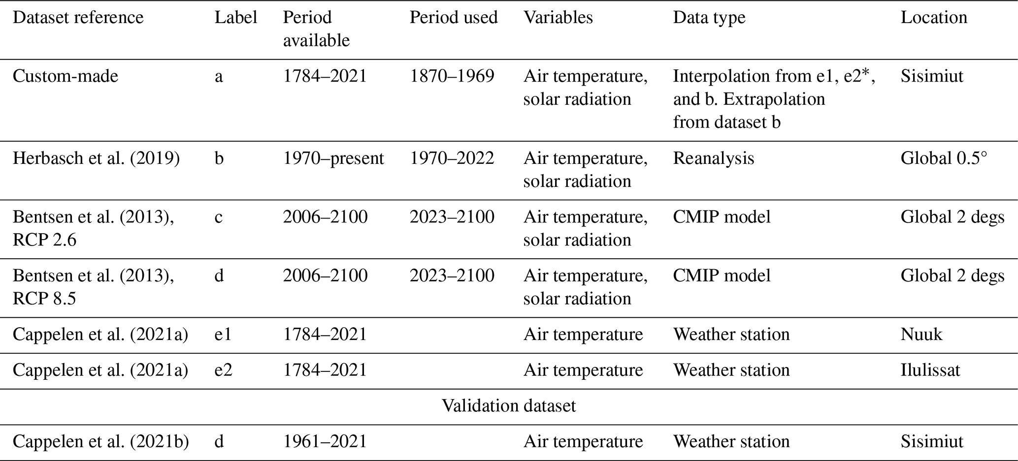
^* Used to generate air temperature of dataset a.

3.3.2 Rock surface temperature modelling

In this step, we model the relationship between downscaled weather data and RST data using a conceptually identical approach to Magnin et al. (2019). The RST is predicted by an empirical model trained using available forcing variables that dominate RST distribution on steep rock walls, i.e. AT and SSRD. To do so, we aggregate each RST measurement to the forcing data that occurred during that acquisition time step. RST data from the period 2020–2022 aggregated at monthly time steps are used as a dependent variable. As predictors, we use AT and SSRD from the ERA5 dataset downscaled at the respective logger location. This creates a database of Nx1 targets and Nx2 data points, where N is the number of available RST data.

The RST is modelled using a multinomial linear regression, trained with the MATLAB function fitlm. To evaluate the validation performance, we follow the classic cross-validation approach that iteratively splits the dataset randomly into 80 % training and 20 % validation until all data points are used both as training and validation. To evaluate the test performance, we predict the RST time series at the borehole SIS2021-01 location and compare it to the data measured at 0.1 m depth which are not used for the training and validation routine.

3.3.3 Heat transfer model

To describe deep rock temperatures, we develop a 1D numerical model that we calibrate with SIS2021-01 borehole data. In this study, we use COMSOL Multiphysics^® heat transfer module (COMSOL Inc., 2015). The heat transfer is modelled using the “heat transfer in porous media” module in COMSOL, which assumes the local thermal equilibrium hypothesis to be valid and simulates conduction only. The model geometry consists of a 100 m 1D model. The model accounts for three materials: solid matrix, fluid, and solid with phase change. The fluid phase is the default COMSOL “water” material, to which we assigned a phase change to ice at 273.15 K and a transition interval to ice of 2 K, according to Noetzli and Gruber (2009). The matrix density is assigned in agreement with the data from the core extracted from SIS2021-01. The data show an increase from 2600 to 3000 kg m⁻³ at 20 m b.g.s. and then remain constant thereafter.

Since we do not have precise information on the rock thermal properties, we calibrate the specific heat capacity, thermal conductivity, and matrix porosity of the solid phase. The calibration is carried out by simulating conditions in SIS2021-01 from 1870 to 2022 using 1D geometry of a 100 m column. The simulation results are then compared to the field data acquired during the period August 2021 to April 2022. This is repeated for different combinations of thermal properties, targeting the minimization of the RMSE between the measured and modelled temperatures across the borehole depth.

The numerical simulation consists of three successive studies: a stationary study for initial conditions (mean conditions for 1870–1890, forcing dataset a), a transient study for 1870–1969 (forcing dataset a), and a transient study for 1970–2022 (forcing dataset b). All weather datasets are downscaled at the desired location using the TopoSCALE algorithm, as described in Sect. 3.3.1. The corresponding RST time series is computed using the RST model developed in Sect. 3.3.2 and used as surface boundary condition.

As a lower boundary condition, we impose the constant geothermal heat flux, which we evaluated from the temperature gradient of 0.015 °C m⁻¹ measured from 100 to 90 m b.g.s. at SIS2021-01. As initial conditions, we compute the temperature profile of the stationary solution of the 1D model forced by the average RST over the period 1870–1890. We then add a positive ground temperature offset as a parameter to account for the fact that temperatures in 1870–1890 (at the Little Ice Age peak) were lower than the previous period and that deep ground temperatures were likely higher than modelled by our stationary model. This temperature offset is also matter of calibration.

3.3.4 Model testing

To test the performance of the numerical model, we simulate rock temperatures using the calibrated thermal characteristics and RST boundary conditions downscaled at the SIS2019-02 and the ERT transect. The former simulation is set up using the 1D geometry described in the previous section. The latter simulation is set up using 2D geometry along a north–south transect extracted from the digital elevation model using QGIS (Quantum GIS; QGIS, 2023). The elevation profile is then imported into COMSOL as 2D geometry using the parametric function option. We then evaluate the RST forcing independently at each profile node using the approach described in Sect. 3.3.2. The RST time series are then parameterized as a function of the spatial variable (x) and temporal variable (t) and used as a surface boundary condition for the 2D model. As a lower boundary condition, we impose the geothermal heat flux evaluated from the borehole SIS2021-01, while we impose zero-flux conditions on the lateral boundaries.

3.4 Permafrost distribution and evolution

In this last section, we explore the present and future distribution of rock wall permafrost in the study area using the modelling tools we have developed in the previous steps. At first, we use the RST model to compute rock wall temperature maps. These maps allow us to visualize the potential distribution of rock wall permafrost. To do so, we first define the rock walls from the digital elevation model as terrain steeper than 40° (Magnin et al., 2019). At the study site, 9.32 km² is steeper than 40° and classified as rock walls. For each grid cell that qualifies as a rock wall, we then compute the RST time series by predicting the RST model on the downscaled AT and SSRD time series for both the current period and the future scenarios. The rock wall temperature maps are then computed by evaluating the mean RST (MRST) for the period 2002–2022 and for the period 2080–2100 using both scenarios RCP 2.6 and RCP 8.5.

In our second analysis, we focus on predicting the future evolution of deep rock temperatures at the SIS2021-01 location. Given that our numerical model is calibrated to fit the data collected at this very site, the level of uncertainty here is arguably at its minimum. To do so, we append two independent transient studies to the heat transfer model generated in Sect. 3.3.3. As an upper boundary condition, we use downscaled RST time series for the two climate scenarios (RCP 2.6 and RCP 8.5, datasets c and d in Table 2) from 2023 until 2100. We then compare the generated temperature profiles for 2100 and describe the permafrost evolution at this site.

In our last analysis, we assess the evolution of mountain permafrost in complex terrain using a 2D-modelling approach. Our investigation centres on two specific locations: the ERT transect and the Nasaasaaq summit ridge. The latter site is chosen to observe the expected evolution of rock wall permafrost at the highest elevations in the area. For both locations, we employ 2D models driven by RST time series from 1870 to 2100, which are downscaled along the elevation profiles following the methodology outlined above (Sect. 3.3.4). We conduct the heat transfer model simulations for both RCP scenarios, allowing us to compare their different impacts on rock wall permafrost.

4 Results and discussion

4.1 Rock temperature monitoring

RST data are measured during 2 full years, as loggers were installed in September–October 2020 and data were collected in September–October 2022. Most loggers show sub-zero RST between early October and late May. The lowest RSTs are reached in late March, when several loggers recorded temperatures around −20 °C (see Fig. 2a). The lowest RST (−21.2 °C) is recorded on 25 February 2022 by a logger installed on a north-facing bedrock slope at 314 m a.s.l. The highest RSTs are reached at the end of July, as several loggers recorded temperatures above 25 °C. The data show that the MRST is correlated with elevation and mean SSRD (see Fig. 2b). To show the effect of elevation, we compare two loggers installed on south-facing rock walls, one at 52 m a.s.l. (MRST $=+\mathrm{3.2}$ °C) and one at 522 m a.s.l. (MRST $=+\mathrm{0.6}$ °C), giving an MRST gradient of 0.0055 °C m${}^{{}^{-}\mathrm{1}}$. By comparing loggers installed on rock walls at the same elevation but on opposite aspects, we obtain an MRST offset of 2.2 °C from north- to south-facing slopes.

Borehole temperatures are shown in Fig. 2b and c. SIS2021-01 (see Fig. 2c) shows consistently negative temperatures between 20 and 70 m depth, reaching a minimum of −0.2 °C at 30 m depth. The depth of zero annual amplitude is approximately 10 m b.g.s. Since we measure negative temperatures below this depth, the data from SIS2021-01 indicate the presence of permafrost. In SIS2019-02 (see Fig. 2d), temperature data indicate a minimum temperature of +0.3 °C reached at 30 m depth, and a temperature of +1.0 °C at 100 m depth. The depth of zero annual amplitude is approximately 20 m. Since temperatures are positive below the depth of zero annual amplitude, the measurements at SIS2019-02 indicate the absence of permafrost.

In comparing the contrasting conditions between SIS2019-02 and SIS2021-01, it is important to note that SIS2019-02, situated at the same elevation and in a slightly more shaded location than SIS2021-01, exhibited lower solar radiation levels (90 W m⁻² versus 104 W m⁻²) during the period 1970–2022. Given this difference, one might anticipate that SIS2019-02 would display permafrost conditions, as observed in SIS2021-01. We propose that the temperature data indicate that the presence or absence of permafrost is influenced by the distinct snow cover characteristics at these two sites. In Arctic climates, snow drifts often form early in the season, and these drift patches persist across different seasons (Parr et al., 2020). The early onset of snow cover has a warming effect on the ground, and when this pattern recurs each winter, as is suspected to occur in SIS2019-02, it can result in a warmer ground compared to in a wind-exposed area such as SIS2021-01.

Overall, the temperature data delineate discontinuous permafrost conditions in rock walls and bedrock. Given the range of elevation where permafrost is found, these conditions are similar to those described in northern Norway (69–71 °N), where negative MRST and rock wall permafrost can be found at low elevation on north-facing slopes (Magnin et al., 2019). The temperature offset induced by slope aspect is known to be dependent on latitude, varying from 8 °C in the European Alps (45–46 °N; Magnin et al., 2015a) to 1.5 °C in northern Norway (69–71 °N; Magnin et al., 2019). In coastal climates, previous studies suggested that steep bedrock permafrost could be influenced by other factors than pure solar radiation, such as cloudiness and icing, creating an abnormally low offset in New Zealand (Allen et al., 2009). Despite the fact that the Sisimiut mountain area is coastal, our data suggest that this process is not a relevant factor for rock wall permafrost distribution in the area.

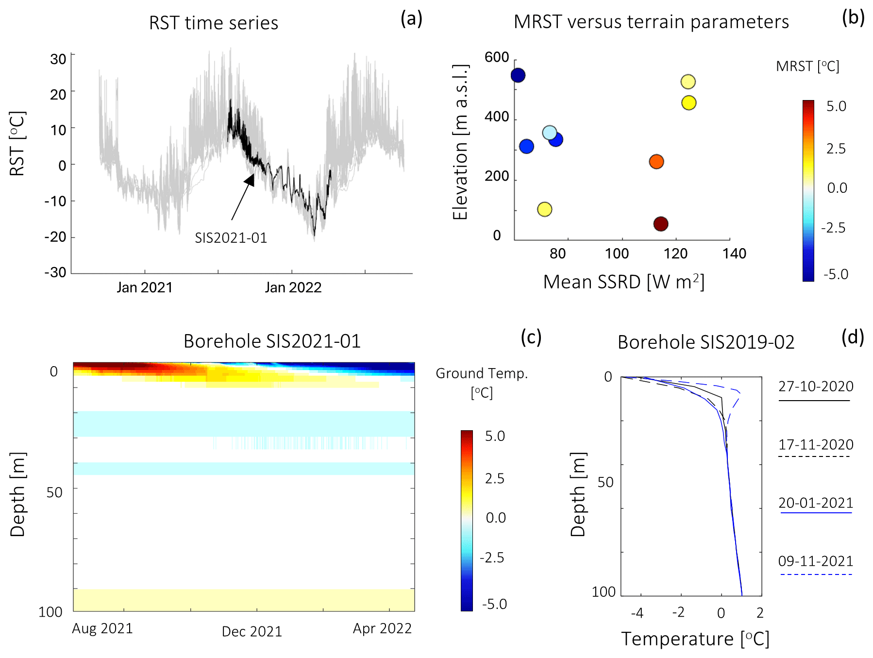
Figure 2 Summary of temperature recorded by the loggers during 2020–2022. (a) RST time series for all loggers. The RST recorded at SIS2021-01 is shown in black; this dataset is used as a test set for the RST model (see Sect. 3.3.2). (b) Relationship between MRST recorded during the observational period (2020–2021) in relation to topographical predictor elevation and mean SSRD during the observational period. Temperature data from boreholes SIS2021-01 (c) and SIS2019-02 (d). For borehole SIS2021-01, data are acquired with an interval of 1 h using an MLog5W-STRING, allowing us to colour-plot temperatures as a function of depth and time. For borehole SIS2019-02, data were measured on four separate dates, using a 5 in. probe lowered manually into the borehole. These measurements produce four temperature profiles, i.e. temperature as a function of depth.

4.2 Geophysical survey

As shown in Fig. 3a, the conductivity values measured along the profile vary from values below 10⁻² up to 10⁻⁶ Sm⁻¹. According to the petrophysical analysis, shown in Fig. 3b, this range of conductivity highlights the co-existence of frozen and unfrozen conditions. Although the precise temperature–conductivity relationship is dependent upon a single sample, the analysis shows a common pattern of a sharp increase in conductivity as soon as a temperature of 0 °C is reached. This feature occurs between 10^−4.4 and 10^−3.5 Sm⁻¹ for all samples. Therefore, this range of conductivity values is used as a threshold to define frozen, unfrozen, and transition zones in the electrical resistivity (ER) tomogram. In the transition zone, our analysis is not able to discern between frozen and unfrozen conditions.

When applying these thresholds to the ERT field data, we can describe the patterns of frozen and unfrozen conditions of the mountain (see Fig. 3a). Frozen conditions occur in the central section of the north face at 300–350 m a.s.l. The frozen area reaches depths well below the depth of zero annual amplitude, indicating the presence of permafrost at this location. The summit and most of the south face are in transitioning conditions, indicating warmer temperatures than the central section of the north face. The south face is also characterized by a large unfrozen body, which we interpret as the absence of permafrost in the rock wall.

Unfrozen conditions are also shown on the lower section of the north face below 300 m a.s.l. The presence of unfrozen conditions at this location is in contrast with our understanding of permafrost distribution in the area. Permafrost is expected to exist on north-facing steep terrain already at low elevation, as highlighted by RST and borehole data described in the previous section. Additionally, since this location is characterized by north-facing aspect and higher elevation compared to SIS2021-01, we would expect colder conditions than the data collected from the borehole. Although snow may play a warming role as observed in SIS2019-01, this section of the face has slopes that guarantee snow-free conditions throughout the winter. To explain this anomaly, we highlight that this area coincides with a large lithological fault observable in the field. As result, the ER tomogram shows a sharp transition in conductivity values. We suggest that the ERT data at this location are influenced not only by bedrock temperature but also by weathering (resulting from the formation of kaolinite; see Richards et al., 2010) and fracturing. We have assumed that the rock is isotropic and that the laboratory measurements are representative of the scale investigated in the ER tomogram (sensitivity close to the electrode spacing close to the ground surface). Fracturing and weathering challenge the isotropic conditions that are necessary to meaningfully compare laboratory analyses to the ER tomogram. Therefore, we consider the ERT data at this location to be unreliable, and we disregard this area of the tomogram in our further analyses.

Overall, the geophysical survey indicates that, at this location, permafrost is discontinuous. Up to this elevation (400 m a.s.l.), the data describe either frozen or unfrozen conditions depending upon whether we are on a north- or south-facing rock wall respectively. This observation is in agreement with the RST data described in the previous section. The co-existence of frozen, unfrozen, and transitioning conditions suggests that deep permafrost has temperatures close to thawing point. This is in agreement with the borehole data described in the previous section.

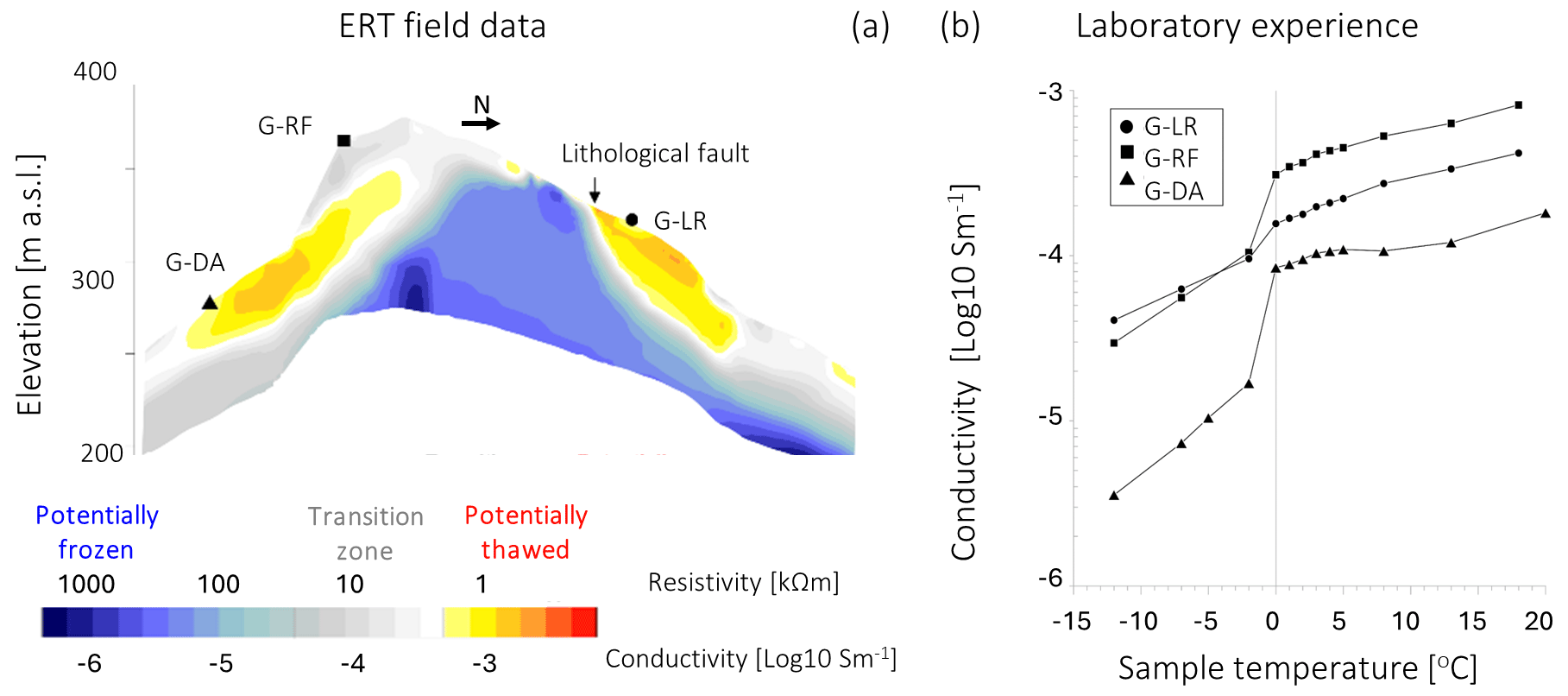
Figure 3 Summary of the geophysical survey. (a) Profile of electrical conductivity/resistivity tomography (in Sm⁻¹ and k Ωm) measured on the field. (b) Petrophysical analysis showing electrical conductivity data versus temperature for the three samples collected along the geophysical profile.

4.3 Modelling

4.3.1 Weather data and downscaling

A sample time series of the available weather data is shown in Fig. 4a, while the validation scatter plots of the AT data are shown in Fig. 4b. The validation indicates an RMSE of 0.95 °C between the AWS AT data and the ERA5 AT downscaled at the weather station location. This value is comparable to previous studies using this dataset in Greenland (Delhasse et al., 2020) and in complex terrain when downscaled with TopoSCALE (Fiddes and Gruber, 2014). The historical database has a similar performance, showing an RMSE of 1.28 °C.

The data from the NorESM1 scenarios have a higher RMSE, indicating a poorer fit between the data and model. We believe this is an intrinsic characteristic of the model, as the mean errors between measured and modelled AT are consistent with the average error over continents declared by Bentsen et al. (2013), i.e. −1.09 °C. This indicates that the dataset, when compared to historical data, tends to underestimate land temperatures.

It is important to note that this analysis quantifies the performance of the AT data at sea level. Since our study evolves in complex terrain, a comprehensive evaluation of the weather database requires weather data at different elevations and including SSRD. Since we do not possess such data, we refer to the work of Fiddes and Gruber (2014), indicating that the TopoSCALE algorithm provides consistent performance across complex terrain. This suggests that we should expect similar data quality at different elevations and aspects. However, a detailed description of this source of uncertainty remains missing at this location.

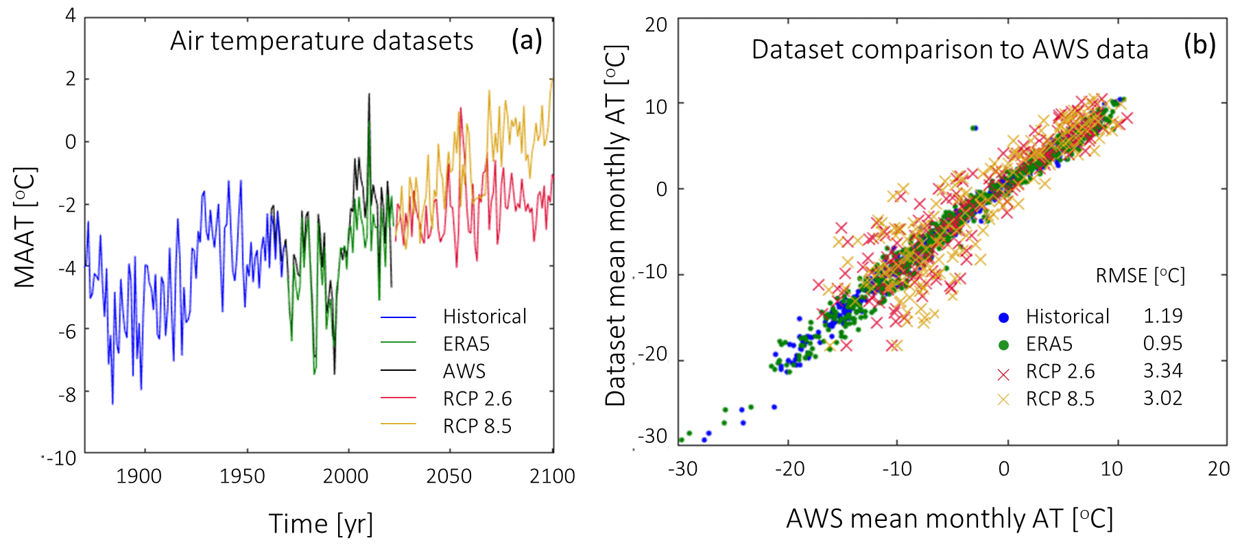
Figure 4 Weather data summary. Yearly time series of the different AT datasets, downscaled at the weather station location (a). Comparison between AWS AT and downscaled AT datasets during the overlapping periods (b).

4.3.2 RST model

The training, validation, and test results of the RST model are summarized in Fig. 5. The model has consistent performance in training, validation, and test results, described by a stable RMSE ranging from 1.99 to 1.96 °C. To better contextualize this performance, we compare our model to that of Schmidt et al. (2021), which represents the state of the art in RST modelling in the Arctic. Their approach is based on the SEB module of CryoGrid 3, modified to account for vertical terrain, including vertical moisture transport affected by latent heat flux and sky view factor adapted to steep terrain. By comparing model runs and field data, Schmidt et al. (2021) obtained R² above 0.97 and an RMSE below 1.20 °C in monthly RST data. This value indicates a better performance than our model. This is likely due to their use of a more sophisticated model and in situ weather station data to force AT. For the sake of comparison, if we force our model with AT from the local AWS, we obtain a lower RMSE, i.e. 1.46 °C, indicating that part of our RMSE is due to the uncertainty of the weather forcing. While it is possible in principle to utilize weather station data to drive our model and enhance its performance, our preference is to evaluate the model uncertainties using data available for the whole of Greenland. This provides an estimation of model performance consistent with the long-term goal to employ this approach for regional-scale use, i.e. in areas where weather station data may not be available.

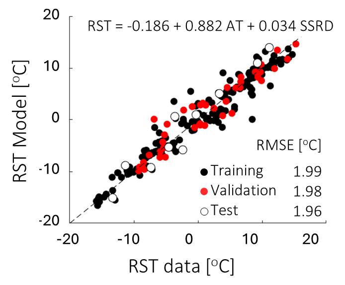
Figure 5 Summary of the RST model. The model is a function of AT and SSRD. Data are aggregated at monthly time steps. Training and validation data are acquired by the RST loggers. Test data are acquired by SIS2021-01.

4.3.3 Heat transfer model

The results of the heat transfer model calibration and validation are summarized in Fig. 6. The calibration of the heat transfer model indicates that the model is mostly sensitive to the porosity value, in agreement with Noetzli and Gruber (2009). According to their study, porosity dominates the sensitivity on short timescales (e.g. decades), while the matrix thermal parameters dominate the sensitivity on longer timescales (e.g. millennia). The calibration yielded an optimal porosity value of 1.5 %, while the optimal initial offset was determined to be +0.8 °C relative to the MRST during the period 1870–1890. The thermal parameters were initially set to the default crystalline rock matrix in COMSOL: thermal conductivity K=2.9 W m⁻¹ K⁻¹ and specific heat capacity C_p=850 J kg⁻¹ K⁻¹. These initial values provided the minimal difference between the model run (Fig. 6a) and the SIS2021-01 data (Fig. 6b) that we managed to achieve. Consequently, we maintain these parameters unaltered from their default settings.

To visualize the model performance, we plot the RMSE distribution between model and data across the borehole depth, as shown in Fig. 6c. The maximum RMSE is measured at 1 m depth (4.02 °C), while it drops consistently lower than 0.20 °C below 10 m b.g.s. When assessing the RMSE throughout the measurement period, we observed values ranging from a maximum of 0.70 °C at the surface to under 0.10 °C at depths less than 10 m b.g.s., further decreasing to under 0.01 °C below 80 m b.g.s. (Fig. 6c). To contextualize the model performance, we compare our results to Magnin et al. (2017), who use a similar transient modelling approach. It must be taken into account that a direct comparison is difficult, as, in our case, boreholes are on flat terrain, while Magnin et al. (2017) have data from boreholes drilled on vertical bedrock, arguably less influenced by lateral variability in ground characteristics and snow cover. Given this, Magnin et al. (2017) also observe large discrepancies between the model and data from the rock surface down to 6 m depth. At 10 m depth, their model has performances varying from 0.70 to 0.01 °C, depending on the borehole and time aggregation used. This indicates that our RMSE is comparable with their findings, further proving that this modelling approach is valuable for predicting rock temperatures where heat transfer is dominated by conduction. Closer to the surface, advective heat transfer, due to water and air circulation in cracks, drives temperature patterns that cannot be modelled by this approach. Although recent studies are developing numerical approaches to quantify these effects (Magnin et al., 2020), it is not currently possible to apply such methods beyond the site scale.

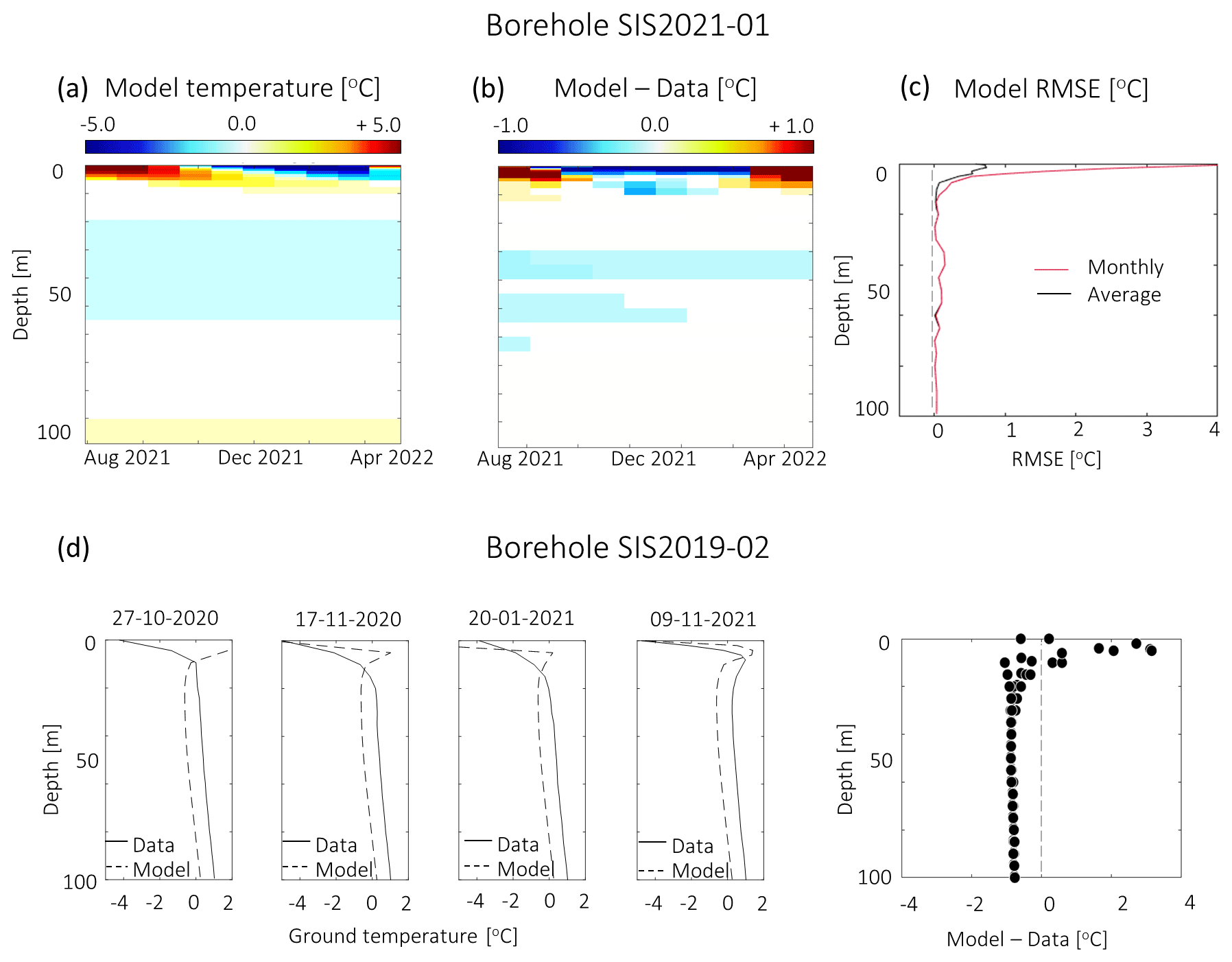
Figure 6 Summary of the heat transfer model calibration and testing with borehole data. All plots are issued by the model calibrated with the parameter values described in Sect. 4.3.3. Heat transfer model run for the observational period of SIS2021-01 (a). Difference between measured temperatures and model results at SIS2021-01 (b). RMSE between model and observations, aggregated at monthly time steps and over the entire observational period (c). Comparison between profile temperatures at SIS2019-01 and summary of model errors in the function of borehole depth (d).

4.3.4 Model testing

When tested and compared to SIS2019-02 (Fig. 6d), the model shows the same error pattern decreasing with depth observed for SIS2021-01, indicating discrepancies up to 2 °C above the depth of zero annual amplitude (20 m depth). Considering that all temperature profiles at this location were recorded in autumn and early winter, it seems that the model overestimates shallow rock temperatures during this period. These cold anomalies in the measured data could be due to advective heat transfer processes in the rock cracks, possibly enhanced by the flat terrain, e.g. cold rain infiltration.

Concerning the temperatures below the depth of zero annual amplitude, the model shows a cold bias, with values 0.85 to 0.75 °C lower than the data. We believe this effect is due to the fact that this borehole is located in an area of recurrent snow drift accumulation, as explained in Sect. 4.1. In particular, our model does not take into account snow accumulation, and it represents ground temperatures in a hypothetical snow-free location with the same AT and SSRD as in SIS2019-02. The difference between our model and the borehole data suggests that recurrent snow cover has a warming effect on deep ground temperatures, which the analysis indicates to be 0.80 °C. Considering this effect, summed to the model RMSE distribution described in the previous section, our model results can deviate −1.0 to 0.2 °C from the data below 10 m b.g.s. This indicates that, when there is snow cover, our model registers colder temperatures compared to the actual deep rock temperatures. This temperature range describes our uncertainty range when predicting rock permafrost conditions in areas where snow may or may not accumulate, i.e. generic bedrock terrain. In the following analysis we will refer to this uncertainty range as the transition zone. Similarly to the transition zone described for the ER tomogram in Sect. 4.2, here our heat transfer model results are uncertain in discerning frozen from unfrozen ground conditions.

As an additional model test, we present the 2D model simulation at the geophysical profile location (Fig. 7). According to the numerical model output, 55 % of the ERT transect area shows frozen ground conditions, while 2 % is expected to be in unfrozen conditions. 43 % of the transect is within the transition zone; i.e. the numerical model predicts a rock temperature within −1.0 to 0.2 °C, and the model is uncertain in assigning either frozen or unfrozen conditions within this range. Similar values are provided by the ER tomogram (48 % frozen, 37 % transition, and 15 % unfrozen). Overall, the model and the ER tomogram have a 74 % agreement, although the model predicts generally colder conditions than indicated by the ERT imaging result.

It is unclear whether our numerical model overestimates permafrost extent or, conversely, whether the interpretation of the ER tomogram underestimates permafrost extent. In particular, the numerical model shows the lower section of the south face of the mountain to be permafrost free, with ground temperatures above zero at 10–20 m depth. Below the summit and towards the south face of the mountain, temperatures are in the range of 0.5 to −1 °C, indicating a transition zone between frozen and unfrozen ground. This pattern of warm south face with transitioning conditions from frozen to unfrozen is in agreement with the ER tomogram, although the latter method shows a larger unfrozen area. The numerical simulation predicts negative temperatures across the whole north face. This pattern is confirmed by the ERT, which shows frozen conditions on the upper part of the face, albeit expecting the unfrozen area to be smaller. As explained in Sect. 4.2, the lower section of the north face is characterized by the presence of a lithological fault affecting the ERT results, and any comparison with the numerical simulation is meaningless here.

Despite these local differences, the two methods agree on the general pattern of permafrost distribution, as they both indicate discontinuous permafrost across the mountain and a dominance of the SSRD in discerning between frozen and unfrozen conditions.

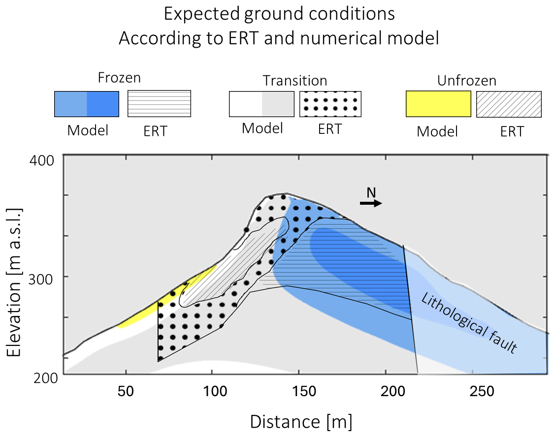
Figure 7 Comparison between the 2D heat transfer model run at the ERT transect location and the interpretation of the ERT imaging result. Ground is described with respect to its conditions, varying from frozen and unfrozen. Transitional conditions indicate the uncertainty range of the two methodologies in discerning frozen from unfrozen ground conditions. The colours indicate ground conditions as described by the heat transfer model, while patterned areas indicate ground conditions as described by the ER tomogram.

4.4 Permafrost distribution and expected evolution

According to our RST model, during the period 2002–2022, 63 % of the rock walls (i.e. 5.85 km²) have negative MRST and likely host permafrost, as summarized in the polar plot in Fig. 8a. North-facing rock walls can reach negative MRST already at sea level, while south-facing rock walls are likely to host permafrost starting at 500 m a.s.l. The colder MRST occurs on the north faces of the Nasaasaaq peak (763 m a.s.l.), reaching −3.0 °C. For the RCP 2.6 simulating the period 2080–2100 (Fig. 8b), there is an increase in the elevation of the MRST 0 °C isotherm of 150 m. This causes a 9 % loss of rock wall permafrost extent from 5.85 to 5.31 km². For the scenario of RCP 8.5 in the period 2080–2100, the impact on permafrost is severe (Fig. 8c), as permanently frozen ground disappears from most of the study area, except for the north faces of the highest summits covering 0.08 km² (less than 1 % of the rock walls in the study area).

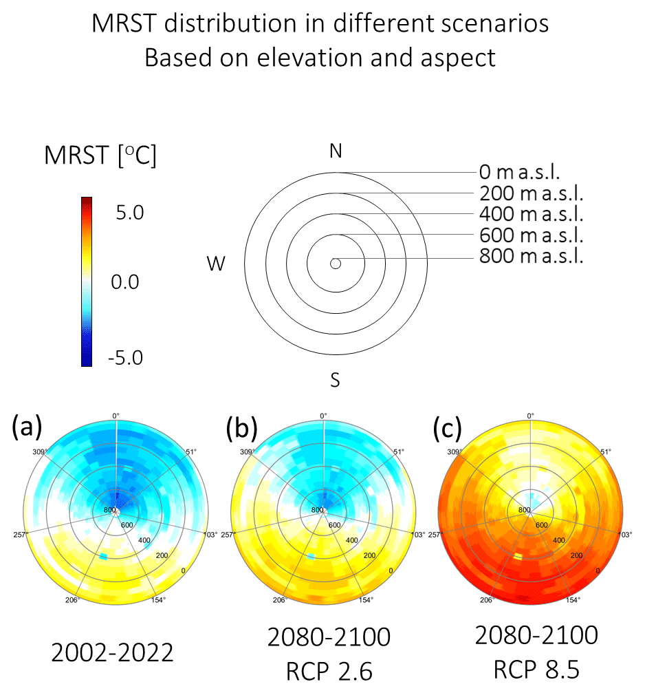
Figure 8 Summary of rock wall MRST distribution at different times and scenarios. The summary is presented as polar plots, where the colour-coded MRST is presented as a function of aspect and elevation. RST distribution is averaged over the periods 2002–2022 (a) and 2080–2010 for scenarios RCP 2.6 (b) and RCP 8.5 (c).

While the MRST maps show the impacts of future climate change on the surface temperatures, numerical simulations quantify the ground temperatures below the surface. The simulations conducted at SIS2021-01 show that, regardless of the scenario used, permafrost conditions will disappear by the end of the 21st century (Fig. 9a). For scenario RCP 2.6, the lowest ground temperature is modelled at 60 m.b.g.s., reaching 0.07 °C (Fig. 9b). For scenario RCP 8.5, ground temperatures are consistently above 0.22 °C (Fig.9b). In 2100, ground temperatures at 20–50 m depth are about 1 to 1.5 °C higher for RCP 8.5 compared to RCP 2.6, indicating that, due to thermal inertia of the ground, surface heat is not yet fully propagated at depth by 2100 in this scenario.

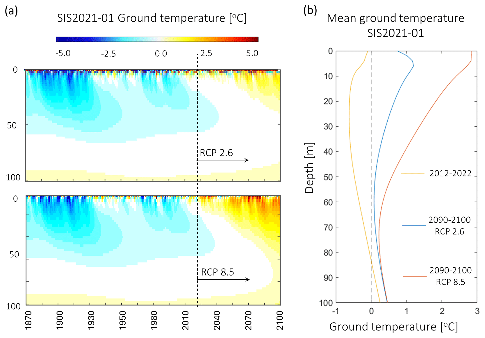
Figure 9 Summary of modelled evolution of temperatures at SIS2021-01. Temperature evolution over the period 1870–2100 depending on the different scenarios (a). Visualization of temperature profiles as a function of borehole depth for different periods and scenarios (b).

A similar result is obtained when evaluating the expected ground temperature evolution in complex terrain by the 2D model (Fig. 10). For the ERT location (Fig. 10a), the model forced with scenario RCP 2.6 suggests an increase in the temperatures of the permafrost body of 0.7 °C, causing minimum ground temperatures to be within our model transition zone. This indicates that, at this location, permafrost is expected to exist at temperatures close to thawing point and only underneath extensive snow-free areas. Scenario RCP 8.5 delineates a situation where transitioning conditions still exist but are constrained below the reach of seasonal frost at approximately 15 m depth below the surface of the north face. Hence, all permafrost on the mountain is relict, as defined by (Magnin et al., 2017), and survives only thanks to the thermal inertia of the ground. The model produces similar results for Nasaasaaq (Fig. 10b), as for scenario RCP 2.6 we observe permafrost retreat to a point that the frozen body is below the reach of the seasonal frost on the whole south face. Scenario RCP 8.5 indicates that all permafrost on the mountain is relict, except for the summit's north face.

The common pattern shown by these results is that the study area is going to experience a reduction in the extent of permafrost in rock walls by 2100, regardless of the scenario considered. This is due to the fact that permafrost in the area is discontinuous and already close to thawing point as of 2022. Even in scenario RCP 2.6, which causes a relatively mild increase in ATs compared to the current conditions, the numerical simulations forecast an increase in deep ground temperatures near 0 °C at mid-elevations (200–400 m a.s.l.). This corresponds to the disappearance of permafrost in most low-elevation south-facing slopes. Scenario RCP 8.5 is expected to have a critical impact on the rock wall permafrost patterns in the area. While permafrost bodies may keep on existing below ground surface even at 200 m a.s.l. (Fig. 10a), less than 1 % of the rock walls is expected to have an MRST below 0 °C by the end of the century, indicating that most rock wall permafrost in the area will become relict. Considering the strong temperature gradients between surface and deep rock temperatures (see RCP 8.5 in Fig. 9b), it is arguable that, even with a stabilization of the climate after 2100, the area will still experience a progressive decrease in rock wall permafrost extent.

These patterns of rock wall permafrost degradation are comparable to the expected evolution of rock wall permafrost at 3400–4000 m a.s.l. in the French Alps described by Magnin et al. (2017). At their location, mountain permafrost is expected to retreat on the highest summits of the Mont Blanc massif, while only relict permafrost can persist at lower elevations. These findings imply that, in the near future, permafrost degradation will affect most of the rock walls in the Sisimiut area, creating the preliminary conditions for a possible increase in rockfall activity of both small and large magnitude (Krautblatter et al., 2013), as observed in the Mont Blanc massif (Ravanel and Deline, 2011).

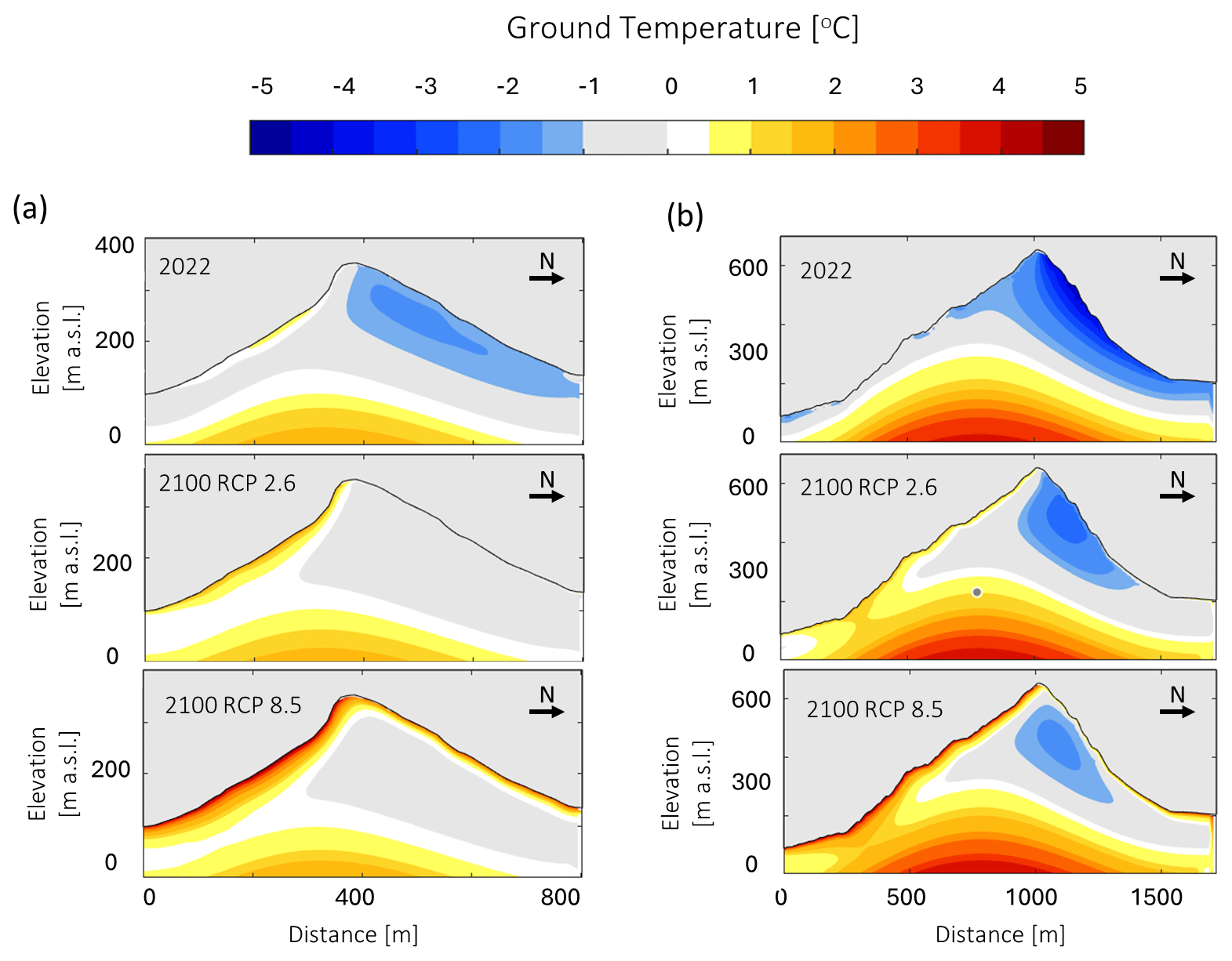
Figure 10 Summary of 2D simulations for future scenarios. 2D models are run until 2100 for RCP 2.6 and RCP 8.5 at the ERT location (a) and the Nasaasaaq summit (b).

5 Conclusions

In this study, we investigate present rock wall permafrost conditions and their expected evolution across the 21st century in the Sisimiut area, West Greenland. Although localized to a small area, we present for the first time an assessment of rock wall permafrost conditions within the country. To describe rock wall permafrost here, we combine different data sources, including RST data, borehole temperatures, geophysical investigations based on ERT, and regionally available weather data. Rock temperatures are simulated using a combination of empirical and numerical models, applied to both 1D and 2D geometries. The main outcomes are the following:

• The data show widespread evidence of discontinuous permafrost in the area. Permafrost can already be found in rock walls and bedrock in shaded locations at sea level. South-facing rock walls are observed to be permafrost-free up to 400 m a.s.l. Measured permafrost temperatures are close to thawing point.

• The modelling results consistently replicate the patterns described by the available data. The modelling uncertainties are of a similar order of magnitude to those observed in previous studies that employed identical methodologies in different geographic locations. This modelling approach is therefore suited to describe permafrost patterns in the study area.

• Considering the optimistic scenario (scenario RCP 2.6), the model predicts a 9 % reduction in the extent of rock wall permafrost by the end of the 21st century. This will affect mostly the south faces, which will become permafrost-free at all elevations in the area. In this scenario, north faces may still host permafrost down to sea level.

• Considering the pessimistic scenario (scenario RCP 8.5), the model predicts a 99 % reduction in the extent of rock wall permafrost by the end of the 21st century. Permafrost will survive only in relict bodies at the core of summits below 600 m a.s.l. MRSTs are expected to be below 0 °C on north-facing rock walls above 600 m a.s.l.

• The current and future state of rock wall permafrost conditions in our study area closely resembles those described in the elevation range of 3300 to 4000 m a.s.l. of the Mont Blanc massif. Consequently, we hypothesize that this ongoing permafrost degradation forms the basis for an increase in rockfall and rockslide activity, as observed in the Mont Blanc area.

Although the correlation between permafrost degradation and rockfall activity is accepted within the scientific community (Ravanel and Deline, 2011; Patton et al., 2019), the process chain linking the two phenomena is very complex. Our modelling approach provides a good first assessment for rock wall permafrost zonation. Additional investigations of slope stability characteristics and their relation to permafrost distribution and degradation could aid in the further refinement of the proposed modelling approach. For potentially endangered slopes, this could be achieved by integrating high-resolution snow distribution (Haberkorn et al., 2017) and crack networks (Magnin et al., 2020), providing a more detailed understanding of slope thermodynamics. Moreover, future research activities should aim towards the application of the proposed modelling approach for investigations at larger scales.