the Creative Commons Attribution 4.0 License.
the Creative Commons Attribution 4.0 License.
 | 12 Apr 2024
Alpine topography of the Gamburtsev Subglacial Mountains, Antarctica, mapped from ice sheet surface morphology
Stewart S. R. Jamieson
Michael J. Bentley
Landscapes buried beneath the Antarctic Ice Sheet preserve information about the geologic and geomorphic evolution of the continent both before and during the wide-scale glaciation that began roughly 34×106 years ago. Since the inception of this ice sheet, some areas have remained cold-based and non-erosive, preserving ancient landscapes remarkably intact. The Gamburtsev Subglacial Mountains in central East Antarctica are one such landscape, maintaining evidence of tectonic, fluvial and glacial controls on their distinctly alpine morphology. The central Gamburtsev Mountains have previously been surveyed using airborne ice-penetrating radar; however, many questions remain as to their evolution and their influence on the East Antarctic Ice Sheet, including where in the region to drill for a 1.5×10⁶ year-long “oldest-ice” core. Here, we derive new maps of the planform geometry of the Gamburtsev Subglacial Mountains from satellite remote sensing datasets of the ice sheet surface, based on the relationship between bed roughness and ice surface morphology. Automated and manual approaches to mapping were tested and validated against existing radar data and elevation models. Manual mapping was more effective than automated approaches at reproducing bed features observed in radar data, but a hybrid approach is suggested for future work. The maps produced here show the detail of mountain ridges and valleys on wavelengths significantly smaller than the spacing of existing radar flightlines, and mapping has extended well beyond the confines of existing radar surveys. Morphometric analysis of the mapped landscape reveals that it constitutes a preserved (>34 Ma) dendritic valley network, with some evidence for modification by topographically confined glaciation prior to ice sheet inception. The planform geometry of the landscape is a significant control on locations of basal melting, subglacial hydrological flows and the stability of the ice sheet over time, so the maps presented here may help to guide decisions about where to search for oldest ice.
- Article
(10746 KB) - Full-text XML
-
Supplement
(1832 KB) - BibTeX
- EndNote


Ice that remains frozen to its bed largely protects subglacial topography from erosion, preserving landscapes formed millions of years ago under climatic conditions and/or ice sheet configurations drastically different to those of the present day (e.g. Jamieson et al., 2005; Young et al., 2011; Rose et al., 2013; Paxman et al., 2018; Franke et al., 2021). Subglacial landscapes can therefore provide unique records of glacial and preglacial geomorphic processes. Their importance as controls on ice sheet initiation, evolution and potential collapse has also been recognised (Sugden and John, 1976; Mercer, 1978; DeConto and Pollard, 2003), and a key focus in recent years has been the production of gridded subglacial topographic datasets that can be used as boundary conditions for ice sheet models (Fretwell et al., 2013; Morlighem et al., 2020; Frémand et al., 2023). Standard methods using airborne ice-penetrating radar (or radio-echo sounding; RES) to measure ice thickness, and hence derive bed elevations, are effective at producing vertical profiles but rely on interpolation techniques (e.g. Morlighem et al., 2011) or the use of coarser-resolution or satellite-derived gravity data (Fretwell et al., 2013) to fill gaps between transects (flightlines). These gaps are rarely smaller than 5–10 km and are often much larger (Fretwell et al., 2013; Pritchard et al., 2014); hence the planform (horizontal) structures of subglacial landscapes may be poorly known at significant scales, even in areas where RES coverage is good.
An approach to mapping subglacial landscapes with the potential to address this issue is the use of ice sheet surface morphology (Le Brocq et al., 2008; Ross et al., 2014; Chang et al., 2016), which records the fingerprint of subglacial topography due to its influence on ice flow (Rémy and Minster, 1997). Changes in slope, or curvature, of the ice surface can be extracted from radar-based satellite imagery (e.g. MODIS and RADARSAT image mosaics; Scambos et al., 2007; Jezek et al., 2013) and digital elevation models (DEMs; e.g. Bamber et al., 2009; Howat et al., 2019) and used to map out the planform geometry of subglacial ridges and valleys over which the modern ice sheet flows. This information can be used to fill gaps between RES surveys (e.g. Ross et al., 2014) or give a preliminary indication of the landscape structure in areas with few existing data (e.g. Le Brocq et al., 2008; Jamieson et al., 2016). Moreover, recent high-resolution datasets, such as the Reference Elevation Model of Antarctica DEM (Howat et al., 2019) and the RADARSAT-1 Antarctic Mapping Project image mosaic (Jezek et al., 2013), offer the possibility to enhance knowledge of the fine-scale topographic structure of ice sheet beds even in areas previously well-surveyed.
One such region is the enigmatic landscape of the Gamburtsev Subglacial Mountains (GSMs) in central East Antarctica. Bounded by the Lambert Graben to the north, the South Pole Basin to the south, and a complex system of linear faults (Ferraccioli et al., 2011) to the east and west (Fig. 1), the GSMs are a high-relief, alpine mountain range (Bo et al., 2009; Rose et al., 2013) entirely submerged beneath Dome A, the highest point of the Antarctic Ice Sheet. Prior to the internationally collaborative Antarctica's Gamburtsev Province (AGAP) project during the International Polar Year of 2007–2009 (Bell et al., 2011; Ferraccioli et al., 2011), very little was known about their structure. Analysis of the RES data collected by the AGAP surveys revealed a dendritic network of subglacial valleys surrounded by large mountain massifs, bearing evidence of multiple stages of glacial modification (Rose et al., 2013). The relatively high level of detail achieved by the AGAP survey does not persist outside of the survey area, but the few existing measurements suggest that the surrounding foothills of the GSMs may be much more extensive. The surveys provide a clear benchmark against which to validate interpretations made from ice surface mapping (see Ross et al., 2014; Jamieson et al., 2016), which may also expand detail of the landscape beyond the surveyed region and in between AGAP flightlines. The high bed relief (Bell et al., 2011; Rose et al., 2013), relatively thin ice and slow ice flow (Mouginot et al., 2019) over the GSMs produce surface expressions that can be mapped to infer landscape structure.
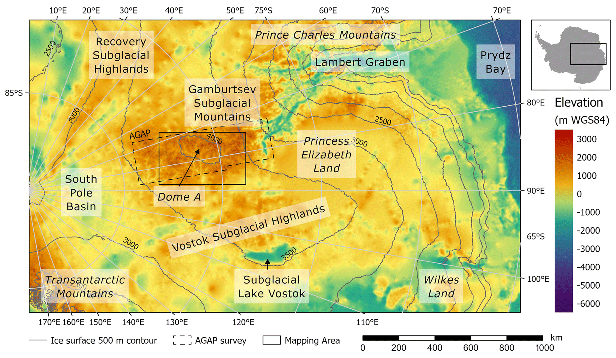
Figure 1The regional subglacial topography of central East Antarctica from Bedmap2 (Fretwell et al., 2013), including place names mentioned in the text. Names in italics are surficial/subaerial features, and names in regular typeface are bed features. The area of interest for this study (Figs. 2, 6, 10) is indicated by the solid box. AGAP signifies Antarctica's Gamburtsev Province.
The aim of this study is to understand the long-term landscape and ice sheet evolution in the Gamburtsev Subglacial Mountains using information about the planform geometry of the landscape mapped from ice surface datasets. Our objectives are (1) to test and compare methods for delineating subglacial ridges and valleys from ice surface datasets, achieved by processing remotely sensed data to derive ice surface curvature and using manual and automated techniques to map changes in slope; (2) to map the subglacial valley and ridge networks of the GSMs, using the methods tested in step 1 with datasets of the Reference Elevation Model of Antarctica (REMA) ice surface DEM (Howat et al., 2019) and the RADARSAT-1 Antarctic Mapping Project (RAMP) image mosaic version 2 (Jezek et al., 2013), both at 200 m spatial resolution; (3) to evaluate the mapped networks against existing bed elevation models and RES data taken from AGAP surveys (Bell et al., 2011; Ferraccioli et al., 2011) and BedMachine Antarctica (Morlighem et al., 2020); (4) to analyse the morphometry of the mapped networks, using metrics including valley length, orientation and spacing; and (5) to interpret the mapped landscape with respect to geomorphic processes and ice sheet behaviour, by assessing the role of different processes (glacial, fluvial, tectonic) in its evolution and its implications for the past and present evolution of the Antarctic Ice Sheet.
Study area: the Gamburtsev Subglacial Mountains (GSMs)
The geology of the Gamburtsev Subglacial Mountains (Fig. 2) is poorly understood, with their location and total submersion beneath the high plateau of the East Antarctic Ice Sheet (Dome A) rendering them currently inaccessible for direct sampling of bedrock. Their origin has been a persistent question since their discovery (Sorokhtin et al., 1959), with debate around the cause and timing of uplift remaining largely unresolved (van de Flierdt et al., 2008; Block et al., 2009; Ferraccioli et al., 2011; Heeszel et al., 2013; Paxman et al., 2016). Several hypotheses have been proposed, including geologically recent thermal uplift associated with mantle hot spot activity (Sleep, 2006), ancient orogeny in a continental collision zone (Fitzsimons, 2000, 2003; Block et al., 2009), crustal shortening in response to long-distance stress transmission (Veevers, 1994) and uplift associated with rifting during continental breakup (Ferraccioli et al., 2011). Attempts have been made to date their formation using detrital materials of likely ancestral GSM provenance from coastal and offshore sediment deposits in the Prince Charles Mountains and Prydz Bay (Veevers and Saeed, 2008; Veevers et al., 2008; van de Flierdt et al., 2008; Gupta et al., 2022), producing ages generally in the ranges ca. 1200–800 Ma and ca. 620–460 Ma (Veevers and Saeed, 2008; van de Flierdt et al., 2008), with another potential period of activity at ca. 700 Ma (Gupta et al., 2022). More recently, dates from intact rock clasts in the Transantarctic Mountains, which may have been transported there subglacially from the GSMs, indicate crustal formation spanning the period of ca. 1100–2000 Ma (Goodge et al., 2017) and a period of rapid cooling at ca. 500 Ma, pointing to exhumation and thus East Antarctic orogeny around this time (Fitzgerald and Goodge, 2022). The landscape of the GSMs has been characterised as predominantly fluvial in origin (Rose et al., 2013), bearing evidence of a dendritic valley network organised into discrete drainage basins, concave valley long profiles and some V-shaped valley forms (Bo et al., 2009; Rose et al., 2013). Modelling (Paxman et al., 2016) based on low rates of erosion (see Cox et al., 2010) suggests that the fluvial network of the GSMs is no more than 230 Myr old.
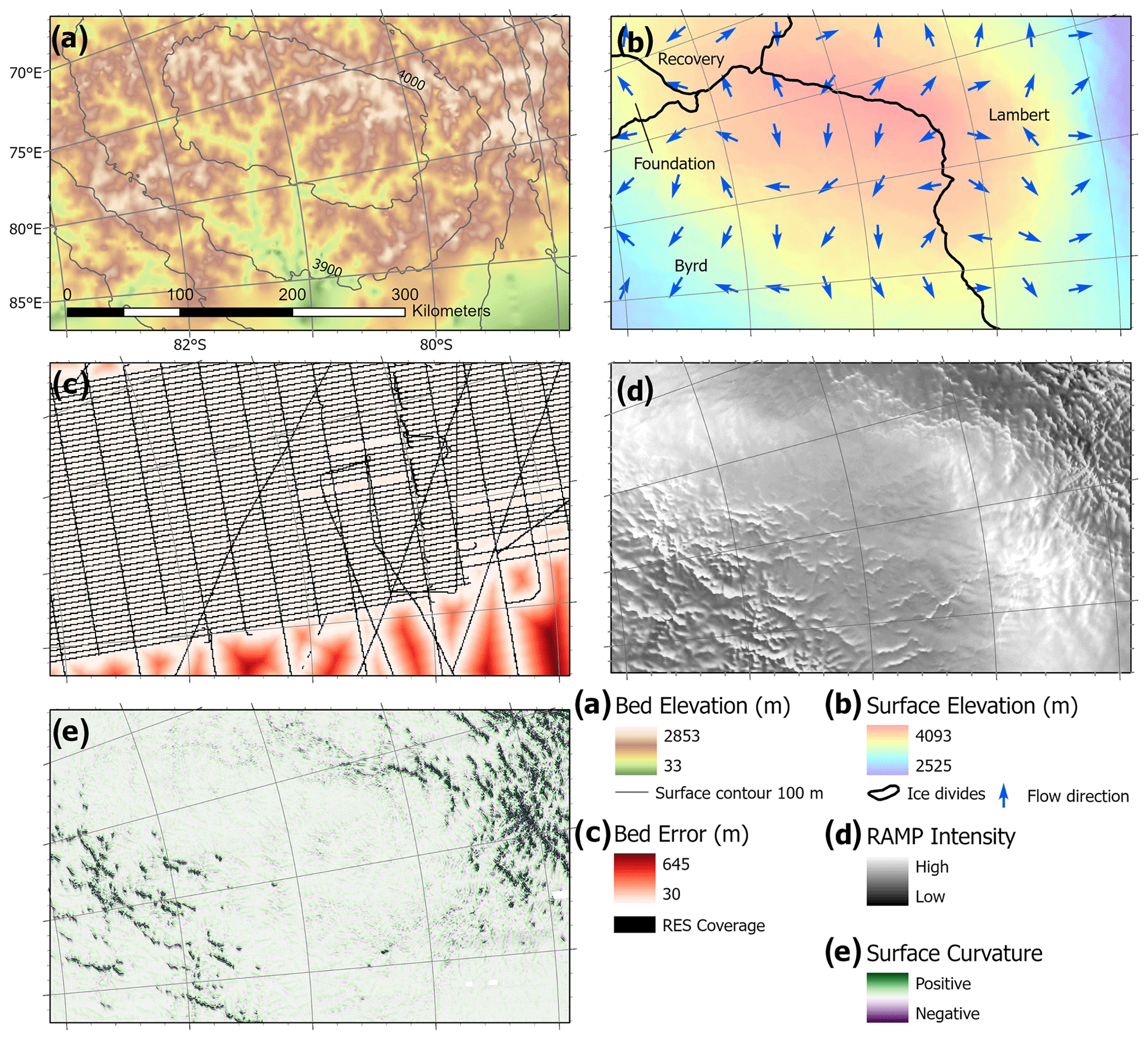
Figure 2Area of the Gamburtsev Subglacial Mountains being targeted for mapping in this study. Bed elevation and errors from BedMachine Antarctica (Morlighem et al., 2020). Surface elevation from Reference Elevation Model of Antarctica (Howat et al., 2019). Flow vectors from MEaSUREs flow velocity (Mouginot et al., 2019). Ice divides (catchments labelled) from Zwally et al. (2012). Radio-echo sounding (RES) flightlines from Fretwell et al. (2013). Satellite image from RADARSAT-1 Antarctic Mapping Project (RAMP) image mosaic version 2 (Jezek et al., 2013).
Evidence is also found for modification of the fluvial landscape by topographically confined, alpine-style glaciation prior to the formation of regional or continental-scale ice caps (Bo et al., 2009; Rose et al., 2013). Glacial landforms present in the landscape, such as U-shaped troughs, overdeepenings, cirques and hanging valleys, are indicative of this style of glaciation and incompatible with formation under modern ice sheet flow. A significant step change in the benthic oxygen isotope ratio is used to place continental ice sheet inception in Antarctica at the Eocene–Oligocene transition at ca. 34 Ma due to the link between increased terrestrial ice volume and greater storage of heavy (18O) isotopes in seawater, leading to higher δ18O in benthic organisms (Coxall et al., 2005). It may therefore be inferred that phases of cirque and alpine-style glaciation in the GSMs were likely associated with periods of climatic cooling that predate this change (Rose et al., 2013), though the exact timing of such episodes remains uncertain. There is growing evidence for fluctuating glaciations in Antarctica during the late Eocene at ca. 38–34 Ma (Van Breedam et al., 2022, and references therein), but some authors argue for the existence of terrestrial ice as far back as the late Cretaceous, at ca. 130 Ma, to explain changes in sea level and ocean chemistry which occurred at that time (Stoll and Schrag, 1996; Miller et al., 2008).
The basal thermal regime is key to patterns of landscape erosion and preservation beneath the Antarctic Ice Sheet (Jamieson et al., 2014), as significant glacial erosion is dependent on the occurrence of basal melting (Sugden and John, 1976). Models suggest that ice in the GSMs has remained cold-based since the early Oligocene (DeConto and Pollard, 2003; Jamieson et al., 2010), leading to minimal rates of erosion. This conclusion is supported by low rates of offshore sedimentation in the catchments down-ice from the GSMs (Cox et al., 2010) and the preservation of the alpine landscape (Bo et al., 2009; Rose et al., 2013). Bright reflections in AGAP RES profiles indicate that meltwater is present in the bottom of some overdeepened valleys of the GSMs where ice flow is slow but confirm that on peaks and valley sides, basal ice remains frozen to the bed (Bell et al., 2011; Wolovick et al., 2013; Creyts et al., 2014).
We used satellite-derived datasets relating to ice surface morphology, in isolation, to map the planform geometry of the central part of the Gamburtsev Subglacial Mountains. We tested both automated and manual approaches to digitising changes in ice surface slope, inferred to represent subglacial valleys and ridges, and assessed the results against the AGAP radar survey bed elevation data (Bell et al., 2011; Ferraccioli et al., 2011) and the BedMachine bed elevation model (Morlighem et al., 2020). We subsequently analysed the morphometric characteristics of the revealed valley and ridge networks in order to investigate the nature of the subglacial landscape. The two principal data products used were (1) the Reference Elevation Model of Antarctica (REMA), Version 1 (REMAv1), a high-resolution, continental-scale digital elevation model (DEM) constructed using stereophotogrammetry from commercial optical satellite imagery (Howat et al., 2019), and (2) the RADARSAT-1 Antarctic Mapping Project (RAMP) AMM-1 Synthetic Aperture Radar (SAR) Image Mosaic of Antarctica, Version 2, representing the radar backscatter intensities recorded by the SAR sensor (Jezek et al., 2013). Both products were used in their 200 m spatial resolution versions for consistency. Data coverage over the study area is very good for both datasets, with data in 99.92 % and 100 % of 200 by 200 m cells for the REMA and RAMP datasets respectively.
2.1 Reference Elevation Model of Antarctica (REMA)
In order to more easily identify subtle changes in surface morphology during mapping, curvature, or the rate of change in slope, was calculated from the REMAv1 DEM using the “Surface Parameters” tool in ArcGIS Pro 2.8.2 (cf. Rémy and Minster, 1997; Le Brocq et al., 2008; Ross et al., 2014). Three distinct versions of surface curvature can be calculated using this tool: (a) profile curvature, which records the rate of change in slope in the direction of the greatest slope at each location (the along-slope direction); (b) plan curvature, which is the same quantity in the perpendicular direction (across-slope); (c) standard (or mean) curvature, which is a mixture of the two. In each case, curvature is calculated from a neighbourhood surrounding each pixel, with the size of the neighbourhood defined by a distance which can be varied to suit the wavelength of variability in the surface. Increasing the neighbourhood distance can reduce the impact of short-wavelength noise, though it may also result in smoothing of sharp contrasts in the data. Several different neighbourhood distances were trialled, resulting in curvature rasters with varying degrees of definition and noise (Fig. 3). Based on a visual comparison of mean curvature outputs, it was judged that a neighbourhood distance of 1000 m provided a curvature dataset with an appropriate balance between minimising noise and avoiding blurring of surface features. The 1000 m neighbourhood distance appeared widely applicable throughout the study area, bearing in mind that levels of noise in the dataset vary significantly.
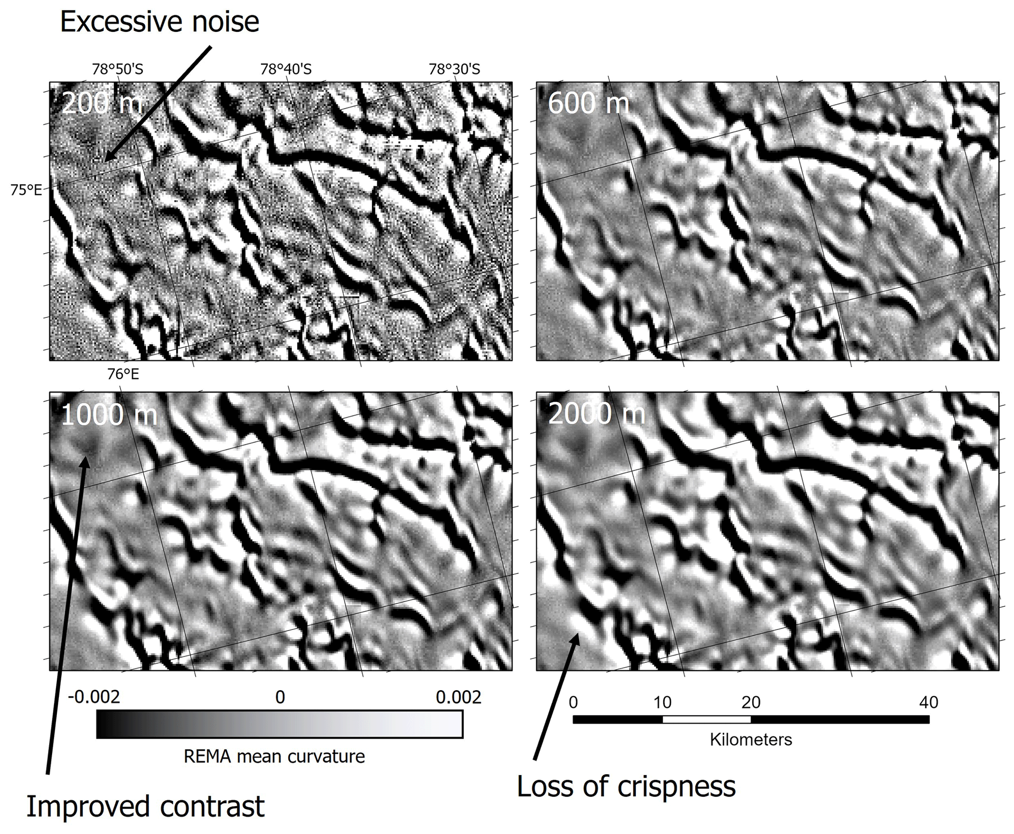
Figure 3Extracts showing normalised mean curvature of REMA surface elevation calculated using different neighbourhood distances (indicated top left of each frame). The 1000 m version (bottom left) was used in all further mapping and analyses. Annotations indicate factors considered in choosing which version to use.
All three curvature products are useful for mapping, as they make it easier to identify the position of greatest slope in a step-change surface feature, represented by the transition from a curvature minimum to a curvature maximum (Fig. 4). For the curvature products used here, a positive value represents convexity (i.e. surface curved upwards), and a negative value represents concavity (i.e. surface curved downwards).
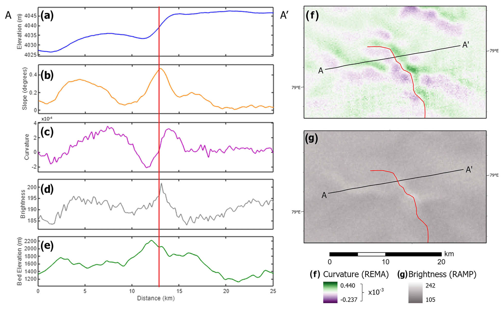
Figure 4Profile (A–A') across a typical ice surface feature (red line), demonstrating the correspondence between the location of a bed ridge and its surface expression in the two datasets used for mapping: (a) Reference Elevation Model of Antarctica (REMA; Howat et al., 2019) surface elevation; (b) REMA surface slope; (c) and (f) REMA surface mean curvature (second derivative); (d) and (g) RADARSAT-1 Antarctic Mapping Project version 2 (RAMP; Jezek et al., 2013) brightness (adjusted backscatter intensity); (e) radio-echo sounding bed elevation from the Antarctica's Gamburtsev Province (AGAP) survey (Bell et al., 2011; Ferraccioli et al., 2011; Corr et al., 2020).
2.2 RADARSAT-1 Antarctic Mapping Project (RAMP)
The pixel values for the RAMP image mosaic represent a qualitative measure of the intensity of radar backscatter (Jezek et al., 2013). The backscatter intensity is useful because it depends in part on the slope angle of the ice surface – a flatter surface leads to more signal being reflected directly back to the sensor and hence a brighter backscatter value (Fig. 4).
2.3 Automated mapping
A variety of approaches to automating the mapping procedure were trialled, with the main aim of identifying edges or contrasts in the input data. The two main approaches tested were (1) thresholding – selectively viewing only portions of the data exceeding certain values in order to isolate, for example, regions of particularly high curvature (cf. Ross et al., 2014; Chang et al., 2016) – and (2) edge detection – using an automated method of identifying sharp contrasts in the data. Key difficulties in both cases included high noise-to-signal ratios in some of the data and large spatial variability in contrast. As a result, a multi-step process was developed, applicable to both the RAMP image mosaic and the REMA mean curvature product (See Supplement for full details). First, an adaptive binary threshold was applied to simplify the input data into a binary mask of “high” and “low” intensity/curvature regions, while accounting for differences in contrast across the study area. Then, a custom-built edge-detection algorithm with a directional input was used to identify and categorise transitions in the binary image. Each pixel was compared with its nearest neighbour in the direction of surface ice flow, and if there was a difference (i.e. the pixel was on an edge oblique to flow direction), it was coded as representing part of a ridge or valley depending on the sign of the change. Additional pre- and post-processing procedures were used to smooth the data and reduce the impact of noise, with slightly different processing steps required for each dataset (See Supplement for full details). InSAR phase-based ice velocities (Mouginot et al., 2019), resampled at 200 m spatial resolution, provided the directional input for the edge-detection step.
2.4 Manual mapping
Manual mapping was conducted using a GIS, with changes in slope being manually traced as vector line features in a geodatabase, with reference to the RAMP image mosaic and all three versions of REMA curvature. An important difference between this approach and the automated procedure was that the manual mapping was conducted as a deliberately interpretive process. Ridges and valleys were digitised separately, distinguished from one another both by the local flow direction with regard to changes in curvature and/or intensity and by the spatial relationships between features. Based on the existing knowledge from RES surveys (Bo et al., 2009; Rose et al., 2013) and initial impressions formed when examining the datasets used for mapping, it was assumed that the planform geometry being mapped would broadly resemble that of an alpine mountain landscape originally shaped by fluvial erosion. As a result of this assumption, inferences could be made which were not feasible to automate, particularly connections between features, such that isolated ridge or valley lines were joined – where small gaps existed – to depict the likely structures of mountain chains and drainage networks. The results from automated mapping suggest that this assumption of a network of valleys and ridges is a reasonable one.
Because they were represented more prominently, ridges in a given area were digitised first, followed by valleys (Fig. S4). Following a similar principle, the most obvious features of each type were traced first, and then subtler features were picked out, especially where these connected with established ridges or valleys. All digitised features were subsequently treated equally, with some exceptions: in places, a connecting feature was inferred with no indication of its presence in any of the mapping data, or (in the case of valleys) two possible connections were marked where there was ambiguity. Such cases mostly arose because the assumption that the landscape would constitute a logical fluvial palaeo-drainage network, if true, occasionally required drainage routes or drainage divides that were not observed. These features were marked as “low confidence” and were later excluded from the dataset when performing some of the morphometric analyses. In the case of valleys, each was digitised from its upper end towards its terminus (usually where it joined another valley) such that the direction of each line would reflect the most likely direction of ice-free palaeo-drainage. Determination of valley direction constituted the only instance in which existing bed models were referred to during mapping, as the theoretical flow direction was not always clear from the two-dimensional network alone. This affected only the direction of the mapped feature and not its position.
2.5 Validation
To assess the accuracy of the surface mapping, the patterns of ridges and valleys were compared to AGAP RES data (Corr et al., 2020) and the BedMachine topography (Morlighem et al., 2020).
2.5.1 RES profiles
The processed AGAP RES data (Corr et al., 2020) were downloaded as point features, and points constituting 12 segments of AGAP flightlines that traversed significant ice surface features within the mapped area were arbitrarily selected. The bed elevation values from these points were extracted and plotted as two-dimensional profiles. The locations of the mapped ridges and valleys from both automated and manual methods that intersected these profiles were identified in a GIS and added to the plots. Peaks and troughs in the bed elevation data with a minimum of 100 m prominence were identified as actual ridges and valleys against which to test the accuracy of the mapped data. A distance cut-off of 2 km was assigned for the matching of a mapped feature with a bed feature, and each mapped feature within this distance of the same type of bed feature was assigned as a match, unless another matching feature was closer. No more than one mapped feature was assigned to each bed feature. An additional cut-off value was introduced to filter out mapped valleys or ridges repeated within 1 km of another mapped feature of the same type. This was necessary, particularly when assessing the automated mapping data, which are sampled from the 200 m masks rather than vector lines to remove multiple instances of the same mapped feature being sampled. Alternative values for this cut-off, as well as for the minimum prominence of sampled bed features and the match cut-off distance, were trialled, but these generally did not have a great effect on the outcome of the matching procedure. Metrics then calculated included the proportion of features successfully matched, the proportion of unmatched mapped features, and the mean offset distance between successfully matched bed features and their mapped locations.
2.5.2 BedMachine DEM
The BedMachine Antarctica version 2 bed DEM (Morlighem et al., 2020), which is primarily derived from the AGAP RES data in this area using the streamline diffusion technique, was used to compare the planform ridge and valley networks derived via manual mapping to existing knowledge of the planform landscape structure. Since no bed elevation data were used during the mapping process, this was an independent test of mapping accuracy, as well as an opportunity to assess whether surface mapping offered any improvement to the level of detail in the observable planform geometry. Qualitative comparisons were made particularly of the level of detail available at scales smaller than those generally resolved in the DEM.
2.6 Morphometric analyses
In order to understand the structure of the landscape, a series of morphometric parameters were calculated using the manually mapped ridge and valley networks, as these proved to be the best mapping outputs during the comparisons detailed above.
The lengths of both valley and ridge features were calculated, binned and plotted as frequency distributions. The orientations (non-directional) of lines were calculated on a segment-by-segment basis, binned and plotted as circular histograms (rose diagrams), using the QGIS Line Direction Histogram Plugin (Tveite, 2015) with the bin totals scaled according to the total length of line rather than the number of line segments. Low-confidence features were included in these calculations; however in the case of ridge features, a second set of histograms was also plotted, containing the lengths and orientations of the low-confidence features only, to see whether there was any difference in directional trend to the overall network. Additionally, for each of these three groups of lines, the angle between each line segment and the local mean ice flow direction was calculated and plotted between 0° (line direction parallel to ice flow) and 90° (line at right angles to ice flow) to assess whether there was a significant relationship between the direction of ice flow and the orientations of the features that could be observed on the ice surface.
Feature spacing statistics were calculated based on the minimum distance of each cell from the nearest valley or ridge line. In each case, this statistic was calculated on a 500 by 500 m grid concordant with BedMachine for the sake of comparability. A local mean was taken using a circular moving window of radius 25 cells (12.5 km) to produce a more meaningful visualisation, from which variation in feature spacing across different regions could be assessed. Since the statistic calculated in the first step is equivalent to half the ridge-to-ridge or valley-to-valley distance, the final statistic was multiplied by 2 to represent the full wavelength of feature spacing.
3.1 Automated mapping
Maps resulting from the automated procedure (Fig. 5) successfully identify linear contrasts in both datasets and are able to some extent to categorise them into those that represent valleys and those that represent ridges. There is, however, spatial variation across both datasets in how comprehensively these two tasks are achieved, which makes visual interpretation more difficult and prevents their use in detailed analysis of the valley and ridge networks without further processing. Compared to manual mapping (Fig. 5b), coverage is poorer for both the RAMP and REMA automated maps, and features are not always mapped continuously. Moreover, the classification of features as ridges or valleys is not always consistent, with some features appearing to switch part-way along their length. As a result, the automated maps do not capture the interconnectivity necessary to assess the planform geometry on a larger scale – further processing, likely manual, would be necessary to infer from them the regional networks of subglacial valleys and ridges.
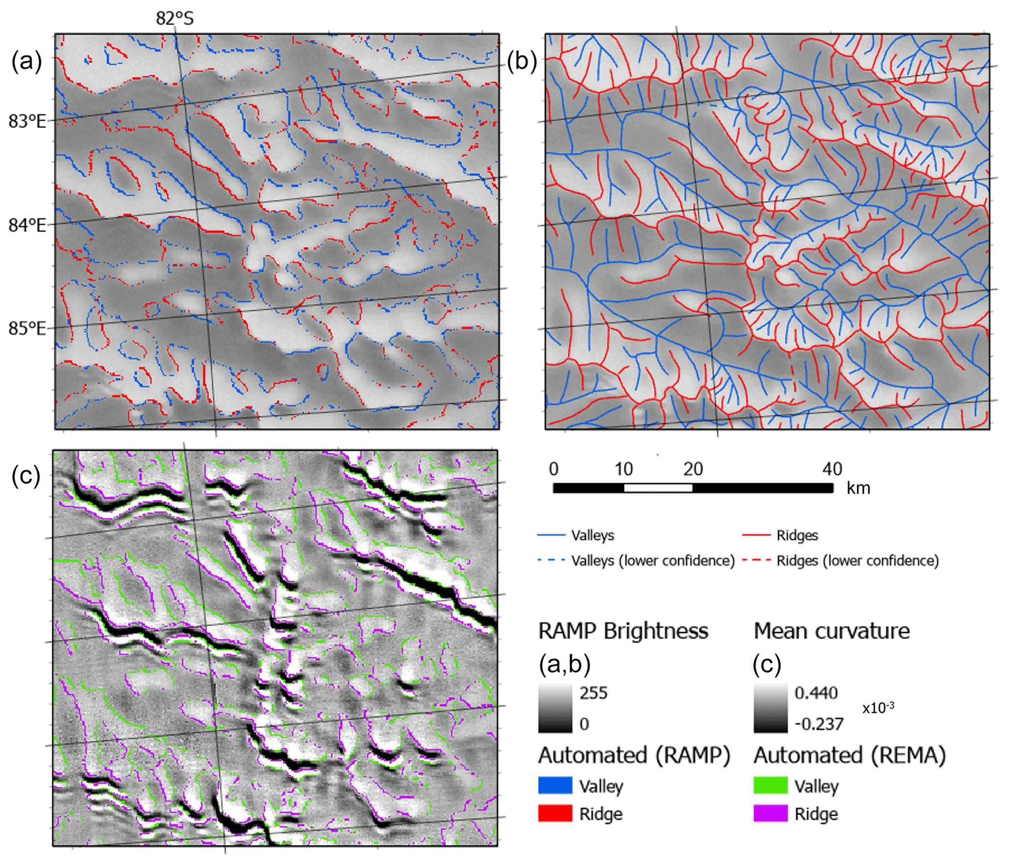
Figure 5Extract from (a) automated mapping using RAMP (RADARSAT-1 Antarctic Mapping Project) image mosaic (underlain); (b) manual mapping using all datasets (RAMP underlain); and (c) automated mapping using REMA (Reference Elevation Model of Antarctica) mean curvature (underlain). Maps in (a) and (c) take the form of 200 m masks of ridge and valley locations and in (b) vector lines tracing ridge and valley networks. Location of extract shown in Fig. 6.
3.2 Manual mapping
The manually digitised map (Fig. 6) reveals a dendritic valley network, centred around two long central valleys, running roughly west to east. Under ice-free conditions, these valleys would form the principal drainage arteries of the mapped area (Rose et al., 2013). Where they converge, at roughly 81° S, 85° E, they have a combined upstream area of approximately 68 700 km2, more than the next largest drainage unit by an order of magnitude. Several other notably long, straight valleys within this region have orientations roughly southwest to northeast. Outside of the central basin, valleys appear to radiate outwards towards the lower-elevation peripheries of the Gamburtsev Subglacial Mountains, including the parts of the mapped area outside the densely sampled central grid of the AGAP RES survey (Bell et al., 2011; Ferraccioli et al., 2011).
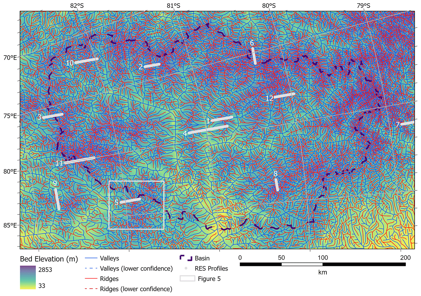
Figure 6Mapped ridge and valley networks in the study area, overlaid on BedMachine Antarctica bed elevation (Morlighem et al., 2020). Radio-echo sounding (RES) profile locations correspond to Fig. 7.
3.3 Validation
The level of detail revealed by manual mapping is a significant improvement on the previous best knowledge of the planform geometry of this area, as seen in the BedMachine DEM, particularly in upland areas, where the frequency of ridges and valleys is below the 5 km minimum line spacing of the AGAP survey grid (Fig. 6). Since the areas of highest bed elevation closely correspond with where ice is thinnest, it is worth noting that the mapping of smaller features in these areas when compared with areas beneath thicker ice may be due to the damping effect of thicker ice on disturbances in flow caused by bed undulations or by differences in flow caused by differences in basal conditions. However, given the assumption that the valley network does represent what was once a fluvial drainage system, it seems probable that there is to some extent a real change in the frequency of valleys and ridges with elevation, as would be expected from a fluvially incised landscape.
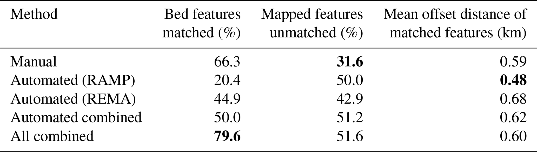
A total of 98 bed features were identified from 12 RES profiles (Fig. 7), comprising 50 valleys and 48 ridges; 79.6 % of these features were successfully identified by at least one method, either manual or automated, with 66.3 % matched to a manually mapped feature and 50.0 % being matched in one or both automated maps (Fig. 8a). This demonstrates the advantage of using multiple datasets in the mapping process and may suggest that in future, a hybrid mapping approach involving both automated and manual interpretive steps offers the most comprehensive method of identifying bed features from ice surface data. Among the manually mapped features along the sampled profiles, 31.6 % were not matched with the indicated type of bed feature (Table 1). Compared with the figures for the automated maps (50.0 % for RAMP and 42.9 % for REMA), this demonstrates the advantage of manual mapping when it comes to avoiding erroneously mapping surface features that are not produced by topographic disruptions to flow or that are in fact artefacts in the mapping datasets. Manual mapping also resulted in the smallest mean horizontal offset for successfully matched features (590 m), with 80 % of offsets no more than 1 km (Fig. 8b).
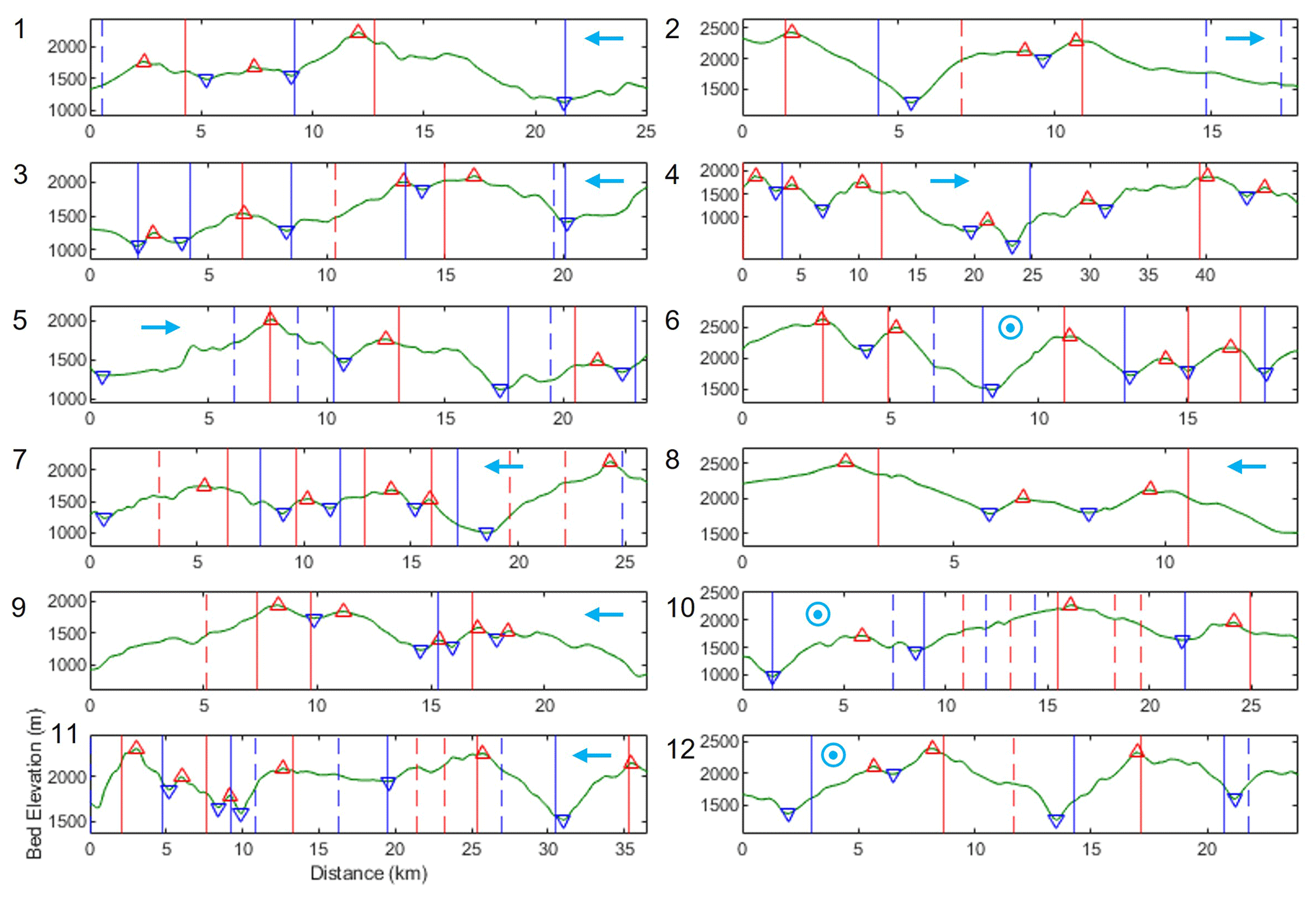
Figure 7Bed profiles sampled from AGAP RES survey (Bell et al., 2011; Ferraccioli et al., 2011; Corr et al., 2020). Peaks (red triangles) and troughs (inverted blue triangles) with >100 m prominence are shown along with the locations of manually mapped ridges (red vertical lines) and valleys (blue vertical lines). A matched feature is denoted by a solid line and unmatched one by a dashed line. Approximate ice flow directions shown by cyan arrows (circle indicates flow out of the page). For profile locations see Fig. 6.
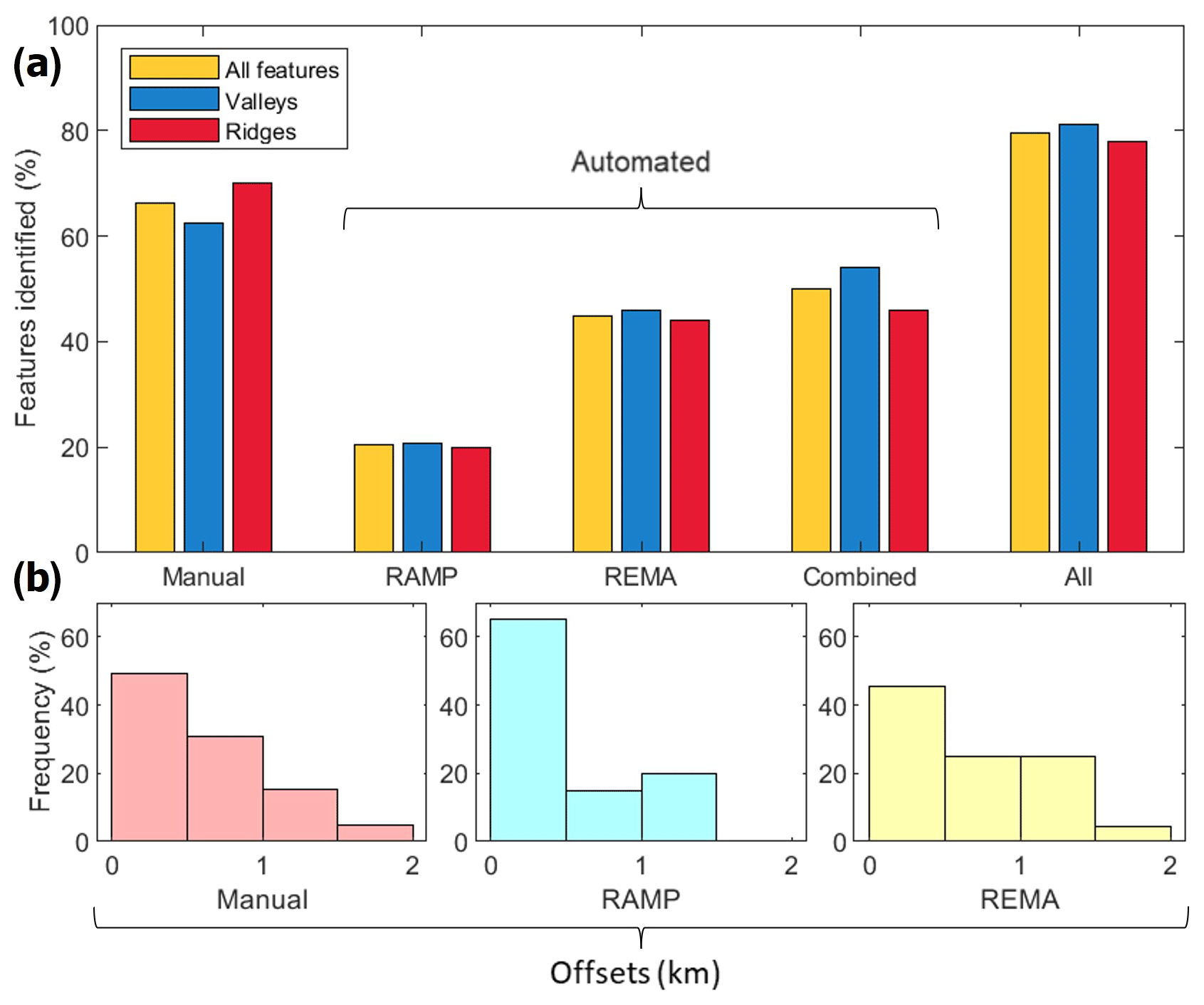
Figure 8Metrics of mapping accuracy, based on 12 sample AGAP radio-echo sounding bed profiles: (a) percentage of bed features successfully identified and (b) frequency distributions of horizontal offsets in mapped locations of bed features.
Table 1Comparing the effectiveness of manual and automated methods in identifying bed features found in selected radar flightlines from the AGAP survey. The optimal value in each column is highlighted in bold.
The variable ability of the method to pick up smaller-scale features is a result of the spatial variability in the degree to which the topography is transferred to the surface (see Chang et al., 2016), which depends not only on ice thickness, but also direction of ice flow (see Ockenden et al., 2022) and other factors such as distance from the ice divide; e.g. Fig. 2d shows how RAMP intensity has greater contrast further from the ice divide, reflecting overall steeper ice surface slopes further from the Dome A summit. As many features as possible were digitised in each region, but the maximal “resolution” of the manual method thus varies spatially. It is notable that decreasing the minimum prominence of peaks and troughs in the bed data to 50 m resulted in many more actual ridges and valleys being identified, which in some places correspond to mapped features that are otherwise unmatched. However, due to the spatial variability in the input datasets, the ability to map features of this scale is not generally consistent across all the profiles; hence, the overall accuracy when considering bed features of this scale is reduced by around 10 % for manually mapped features (the difference is less for the automated methods). Increasing the minimum prominence to 200 m results in a greater proportion of the bed features being successfully matched – more than 90 % of features at this scale were successfully identified by one or more methods – however the number of unmatched manually mapped features increases to 48 % (with similar increases for the automated methods).
3.4 Morphometry
The total set of manually mapped valleys and ridges range in length from less than 1 km to nearly 250 km; however the overall distribution in both cases is log-normal (Fig. 9a), with 61 % of valleys and 55 % of ridges between 1 and 5 km long, rising to 90 % and 85 % respectively between 1 and 15 km. This is largely due to the abundance of short features in higher-elevation areas.
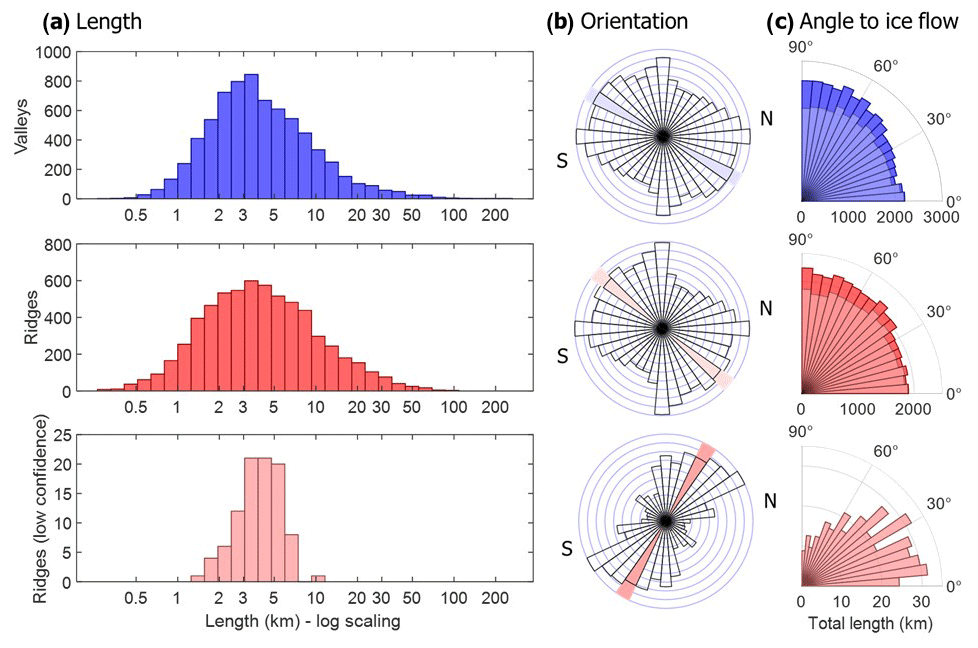
Figure 9(a) Length and (b) orientation of mapped valleys (blue), ridges (red) and lower-confidence ridges only (pink); (c) angle between mapped valleys and ridges and local mean ice flow direction (derived from Mouginot et al., 2019). Shaded bars in (b) denote mean of binned orientations. Horizontal axes in (a) are scaled logarithmically, and radial axes in (b) and (c) record total length of valley and ridge line rather than number of features. Inner bars in the top two plots in (c) represent the baseline after removal of the increasing trend from 0 to 90°. Peaks in orientation at top, bottom, left and right of the top two plots in (b) are artefacts introduced by the pixelation of the input data.
The orientations of ridges and valleys are similar, trending on average roughly southwest to northeast (Fig. 9b). This orientation is roughly concordant with the Dome A ice divide that lies over the northern ridge of the GSMs and roughly perpendicular to the predominant ice flow directions (Fig. 2b). Features oriented perpendicular to flow are more likely to be transmitted to the surface because they present a greater obstacle to flow than those oriented parallel (Ockenden et al., 2022). Comparison between feature orientations and local ice flow directions (Fig. 9c) indicates significant positive correlations between angle from flow and total length of valleys (p=0.93) and ridges (p=0.92), with 30 % and 21 % increases in the value of the linear least-squares fit between 0° and 90° respectively. In both cases, however, the residual is evenly distributed () and accounts for 87 % and 90 % of the total length of valleys and ridges, indicating that overall the mapping is not significantly biased by ice flow direction. The “lower-confidence” ridges display an opposite trend, with a clear preference for northwest-to-southeast orientations. The trend in angle to ice flow is also reversed, showing that these ridges are in general more closely aligned to ice flow. This supports the suggestion that these features exist and that their absence of expression from the surface datasets is due to smoother ice flow associated with this alignment of orientation.
Valley widths generally range between 1 and 15 km; however the local mean for 72 % of the mapped area lies between 1.5 and 2.5 km and is greater than 3 km for less than 2 % (Fig. 10). Valley widths in these upland areas are consistently less than 5 km, which is the minimum spacing of RES survey lines throughout this region. The northern block of the GSMs in particular displays a high density of very narrow valleys, with local means dipping below 1 km in an area that coincides with the mapped region's highest bed elevations (Fig. 10b).
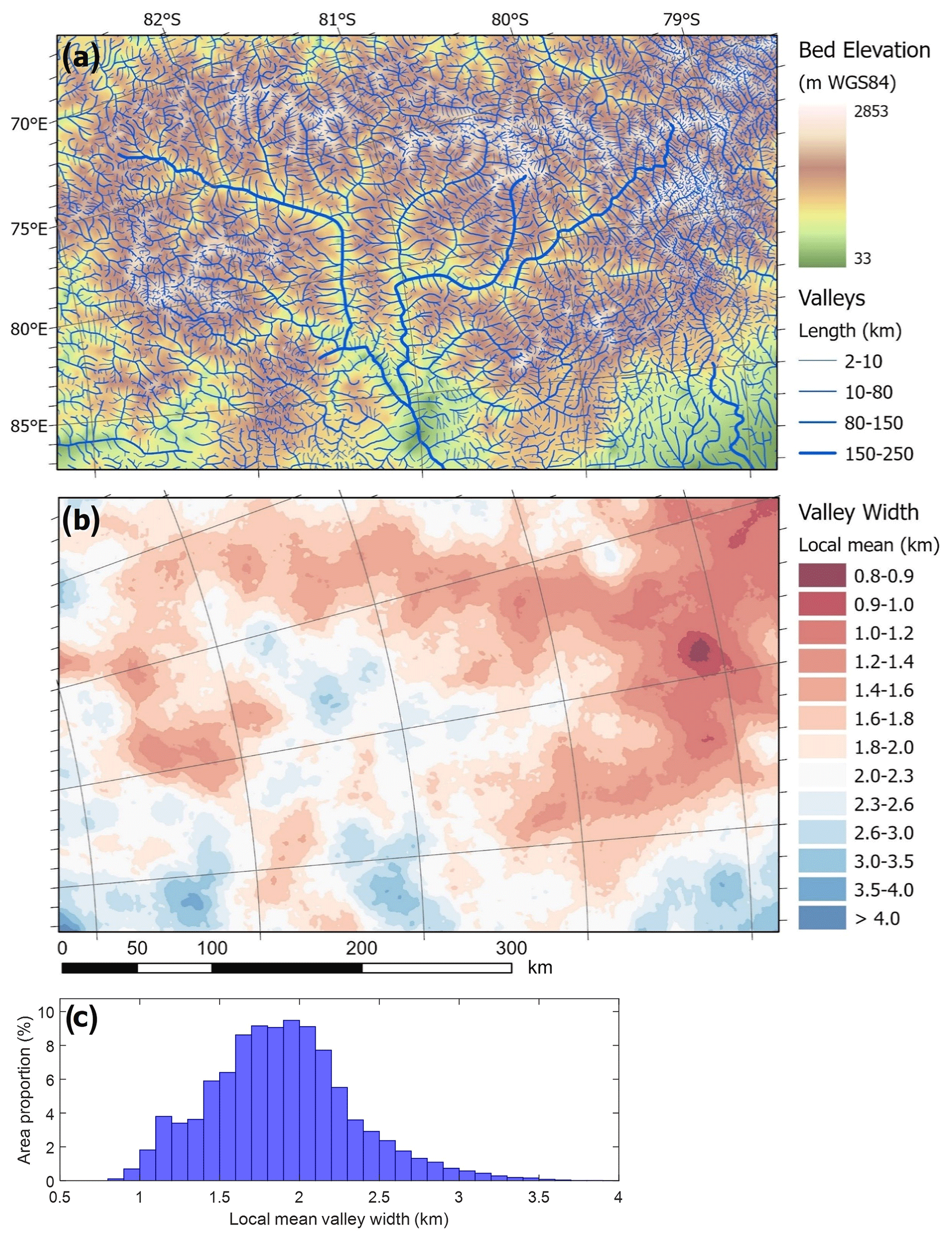
Figure 10Valley morphometry in the central Gamburtsev Subglacial Mountains: (a) mapped valley network, overlaid on BedMachine Antarctica version 2 bed elevation (Morlighem et al., 2020); (b) local mean valley width, calculated from network in (a) as moving-window mean of twice the shortest distance to a mapped valley; (c) frequency distribution of (b).
4.1 Landscape evolution
The mapped valley network bears a predominantly fluvial signature in the form of a dendritic structure, with identifiable drainage units and a drainage density consistent with that for an alpine environment (Fig. 6). The valley network extends further than previously detected, maintaining the fluvial signature beyond the central high-elevation region of the GSMs into the foothills on the eastern side. This is significant for evincing wider-scale drainage patterns in pre-glacial Antarctica. There is also a greater frequency of small tributary valleys in upland areas than previously mapped, improving the detail of the fluvial network in its source regions. High-elevation valley spacing in the central GSMs is generally between 1 and 3 km (Fig. 10), which is directly comparable to first-order valley spacing in alpine mountain ranges: three North American ranges investigated by Pelletier et al. (2010) displayed periodic spacing of first-order valleys between 1 and 3 km, with relief of around 0.5 km. While the mapping conducted here cannot provide valley relief, observation of RES profile data (e.g. Fig. 7) suggests that the relief in the GSMs is also similar. Hence these mountain ranges may provide apt analogues for the scale of valleys present in the GSMs. Previous reconstructions of the topography of the GSMs (Bo et al., 2009; Rose et al., 2013; Morlighem et al., 2020) have not generally resolved valleys this small, despite features of this size being apparent in RES profiles (Bell et al., 2011). Valley widths may be prone to overestimation in RES profiles because radar flightlines often intersect valleys obliquely; knowledge of the planform geometry of the valley network is therefore useful in identifying true cross-sections of valley morphology (see Rose et al., 2013).
Unlike other high-elevation mountain ranges, the GSMs are inferred to be geologically ancient (van de Flierdt et al., 2008; Veevers and Saeed, 2008) and tectonically inactive (Boger, 2011), pre-dating the onset of widespread glaciation in Antarctica at the Eocene–Oligocene transition at 33.7 Ma (Miller et al., 2008; Scher et al., 2011). Given that the GSMs are very unlikely to have been deglaciated since this time (Jamieson et al., 2010), it is reasonable to assume that the mapped fluvial network also predates 33.7 Ma (Rose et al., 2013; Paxman et al., 2016), having subsequently been preserved beneath continually cold-based, non-erosive ice (Van Liefferinge and Pattyn, 2013). The maximum age calculated for this landscape of 230 Ma (Paxman et al., 2016), based on minimal erosion rates (Cox et al., 2010), implies uplift of the GSMs much more recently than is otherwise suggested by detrital thermochronology of Prydz Bay marine sediments (van de Flierdt et al., 2008; Veevers and Saeed, 2008; Gupta et al., 2022) but potentially consistent with cooling histories of subglacial cobbles derived from the interior of East Antarctica (Fitzgerald and Goodge, 2022). The Prydz Bay sediments are presumed to have been sourced from the northern GSMs via the Lambert Graben; however, the valley network (Fig. 6) indicates that although some sediment would travel by that route, it would not have been the predominant route for sediments eroded from the central and southern GSMs, with the large central basin draining east towards the Ross Sea through what is now the Wilkes Subglacial Basin and/or the Transantarctic Mountains. Moreover, there is evidence of heterogeneity in the landscape structure between the northern block and the rest of the GSMs, with valleys more closely spaced in the north (Fig. 10). This potentially suggests a control exerted by differences in the underlying geology of the two regions; hence the Prydz Bay sediments may not be fully representative of bedrock characteristics across the whole GSMs. It is possible that the subglacial cobbles studied by Goodge et al. (2017) and Fitzgerald and Goodge (2022) represent an East Antarctic crustal region incorporating the southern part of the GSMs, whose history differs from that indicated by Prydz Bay sediments to the north.
An alternative possibility is that protective cold-based glaciation was established in the GSMs much earlier than 34 Ma (Stoll and Schrag, 1996; Miller et al., 2008), a hypothesis that is consistent with low long-term erosion rates (Cox et al., 2010). It has previously been suggested that tropical conditions on Antarctica's coast, as evidenced by the occurrence of coal beds (Turner and Padley, 1991; Holdgate et al., 2005), must preclude glaciation of the continent at this time. There is, however, supporting evidence for seasonal sea ice during the Late Cretaceous (Bowman et al., 2013), suggesting conditions also favourable for terrestrial glaciation. It may be that, with sufficiently strong moisture transport inland, the combination of unusual continentality, high altitude and high latitude that exists in the GSMs allowed for glacial cover of the region even during greenhouse climates (Miller et al., 2008; Cox et al., 2010). In this case, the fluvial network may be much older, potentially dating back to the last known period of mountain building in East Antarctica, at ca. 550–500 Ma (An et al., 2015).
While the planform geometry of the landscape mapped in this study is primarily indicative of fluvial processes, it does provide some support for one or more phases of localised, erosive glaciation, prior to ice sheet initiation, that modified the existing fluvial landscape (see Bo et al., 2009; Rose et al., 2013). Ridges mapped as “lower confidence” (LC), due to their apparent absence from the mapping data despite logical necessity for a coherent fluvial geometry, may represent locations where ridges have been locally removed by glacial erosion (i.e. glacial breaches; Dury, 1957). A few minor features of this type were identified by Rose et al. (2013), predominantly at high elevations along the major mountain ridge lines of the GSMs. Alternatively, they may persist beneath the ice but, because of their alignment to the local direction of ice flow (Fig. 9), present insufficient obstacle to cause an expression visible on the ice surface, as has similarly been observed for small bed perturbations beneath fast-flowing, warm-based ice (Ockenden et al., 2022). The physics of bed-to-surface transmission of topographic roughness in such settings are notably more complex than in the slow-flowing, cold-based ice of the GSMs; nonetheless, these results suggest that the overriding principle (i.e. flow predominantly around rather than over bed features oriented parallel to ice flow) may be similar. Since there is diversity in the orientations of LC features, it may be reasonably supposed that those that lie at greater angles to the direction of ice surface flow are more likely to represent glacial breaches.
4.2 Basal thermal regime
As discussed, the wholesale preservation of the mapped fluvial valley network (Fig. 6) is significant evidence in favour of consistently cold-based conditions in the GSMs throughout their occupation by the East Antarctic Ice Sheet (EAIS; Jamieson et al., 2010; Rose et al., 2013). Several authors therefore suggest that the GSMs may host some of the oldest undisturbed basal ice in Antarctica (Fischer et al., 2013; Van Liefferinge and Pattyn, 2013; Wolovick et al., 2021), making them a promising target for drilling “oldest-ice” cores. Such endeavours include the NSF-funded Center for Oldest Ice Exploration (COLDEX), which began surveying in the southern GSMs during the 2022–2023 Antarctic field season. However, basal melting has been seen to occur on small scales (Wolovick et al., 2013) thanks in part to the effects of local topography concentrating geothermal heat flows into topographic lows (Wolovick et al., 2021). Critically, modelling suggests that ridge–valley relief on wavelengths smaller than the spacing of existing RES flightlines (∼ 5 km in the GSMs) may be enough to induce melting in small-scale upland valleys otherwise assumed to lie within areas of permanently cold-based ice (Wolovick et al., 2021). This presents a difficult problem when searching for ice drilling sites, as currently available data are not sufficient to accurately identify (and avoid) these localised patches of warm-based ice. Given that the detailed planform geometry presented here is not limited by the spacing or coverage of RES data and that it records topographic variability on wavelengths consistently below 5 km (Fig. 10), it may therefore be of use in making the predictions of basal thermal conditions required for selecting potential oldest-ice drilling sites.
4.3 Subglacial hydrology
Subglacial topography is also a control on ice sheet hydrology (Wright et al., 2012; Jamieson et al., 2016). In the GSMs, there is restricted movement of subglacial water along corridors of low hydraulic potential, defined primarily by the high-relief bed topography: while the subglacial hydrological gradient, dictated by ice surface slope, drives the direction of these flows, the routes they take are determined by the existing subglacial valley network (Wolovick et al., 2013). The mapped valley network may therefore be an indicator of the pathways available to subglacial water beneath the modern ice sheet. The subglacial hydrological pathways of the GSMs are predominantly short (Wolovick et al., 2013) and often end in zones of basal refreezing where water is forced up reverse bed slopes under pressure and cools (Bell et al., 2011; Creyts et al., 2014). This occurs on valley sides (where bed topography is transverse to ice surface slope) and in valley heads (where bed topography is aligned with but opposite to surface slope such that subglacial water flows up-valley). In the third case, where bed topography is aligned with and sub-parallel to ice surface slope, longer-distance transport may be possible, uninterrupted by basal refreezing. The major valleys that would have drained the palaeo-GSMs to the east (Fig. 6) are in relative accordance with the direction of ice surface slope, potentially offering a subglacial hydrological connection from the GSMs to the wider EAIS. This may be complicated by the transport of water up reverse bed slopes created by overdeepenings along valley long profiles, which are known in the deep valleys of the GSMs (Bo et al., 2009; Rose et al., 2013) but not possible to infer from planform geometry alone.
4.4 Ice sheet evolution
The preservation of the mapped valley network beyond the central region of the GSMs is significant because it demonstrates that, as inferred in the central GSMs (Bo et al., 2009; Rose et al., 2013), glaciation of the surrounding landscape has been minimally erosive or at least that the pattern of ice flow, and hence the pattern of erosion, has been predominantly guided by the pre-existing fluvial geometry. This is consistent with the idea that the GSMs were a key source of ice during the early Oligocene expansion of glaciation in Antarctica (DeConto and Pollard, 2003) because the marginal regions of an expanding ice cap centred on the GSMs would have been initially thin and topographically confined, like many modern-day Arctic ice caps which have topographically confined outlets (e.g. Baffin Island ice cap, Svalbard, Severnaya Zemlya and margins of southeast Greenland). As these ice margins grew, erosion would have been concentrated along these topographic lows (Sugden and John, 1976), leading to a feedback whereby continued erosion promoted increased flow of ice along the same topographic corridors, further focusing erosive power along these routes (Jamieson et al., 2008; Kessler et al., 2008). Even where ice has not remained exclusively cold-based, therefore, the broad strokes of the fluvial valley network of pre-glacial East Antarctica may be more widely preserved than previously understood, indicating remarkable stability at the core of the EAIS. The accordance between the positions and orientations of the central ridge of the GSMs and the overlying Dome A ice divide (Figs. 2, 6) supports the idea that this spine of high topography may have remained a keystone for the EAIS, preventing the deglaciation of one of its major source regions during climate-induced oscillations (Wolovick et al., 2021).
In this study, a new map of the planform ridge and valley geometry of the central Gamburtsev Subglacial Mountains (GSMs), East Antarctica, was produced by using satellite remote sensing data to identify and interpret changes in ice surface slope. Manual and automated approaches to processing these data were tested, and existing bed elevation datasets were used to validate the correspondence between the resulting maps and the known bed topography. Furthermore, the morphometry of the manually mapped networks was analysed, revealing details about the structure of the pre-glacial fluvial landscape and its subsequent evolution under early phases of Antarctic glaciation. Implications of this increased knowledge of the basal topography for the evolution of the East Antarctic Ice Sheet, preservation of ancient ice and its subglacial hydrological systems were also discussed. Key findings of the work were as follows:
-
Mapping of subglacial topography from ice surface curvature is validated for the GSMs by existing measurements of ice thickness from radio-echo sounding (RES) and an existing model of bed topography produced using the RES data. The maps presented here expand both the coverage and the level of detail available for the planform geometry of the GSMs, particularly in high-bed-elevation and thinner-ice areas.
-
Manual mapping identified a greater proportion of bed features (66.3 %) than automated mapping (50.0 %), produced fewer erroneous identifications, and had smaller offsets between mapped and actual features. The proportion of features successfully identified was increased further (79.6 %) when all methods were considered together, suggesting that future mapping would maximise accuracy and comprehensiveness by combining automated and manual approaches.
-
The mapped valley network preserves information about the pre-glacial fluvial regime, suggesting the former existence of a large central catchment (68 700 km2) draining east towards the Ross Sea.
-
There is some evidence for the modification of the fluvial valley network by local- to regional-scale erosive ice through the breaching of fluvial drainage divides and the overdeepening of valley long profiles; however, uncertainty in the mapping of these features produces ambiguity in their interpretation.
-
Care must be taken when interpreting the data presented here to account for the limitations inherent in mapping bed features from the surface. Orientations of features represented may be biased by the direction of ice flow, with features aligned to flow less likely to produce a surface expression. The detail available also varies with the thickness of the ice column, with thicker ice dampening the effects of subglacial topography on flow. This can lead to ambiguity over the presence or interpretation of mapped features, suggesting the importance of using this approach in conjunction with other methods of mapping ice sheet beds, such as radio-echo sounding.
-
The preservation of the pre-glacial fluvial valley network more widely than previously known indicates, for the area surrounding the GSMs, long-term ice sheet behaviour which is either consistently non-erosive or sufficiently influenced by the bed topography to concentrate erosion in pre-existing topographic lows. This is suggested to document the importance of the GSMs as a centre of growth for the early East Antarctic Ice Sheet and as a stabilising influence during its subsequent evolution.
-
The minimum wavelength of detectable topographic variability (<5 km) is smaller than can be reproduced in bed models using existing data. Ridge and valley structures on this scale may play an important role in governing local fluctuations in bed conditions, including occurrences of basal melting and routing of subglacial water flows. Maps of planform landscape geometry such as those presented here may therefore be useful in evaluating sites for the preservation of oldest-ice (>1 Myr) cores in regions of highly variable subglacial topography.
-
In addition to the applications mentioned, the production of synthesised bed elevation models using the mapped network or through combining the mapped network with existing data has not been attempted but may be an avenue to explore in future. Such products could be of use for ice sheet models that seek to simulate more accurately the effects of high-relief basal topography on ice flow or basal hydrology.
Bedmap2 bed elevation and errors are available for download from the UK Polar Data Centre at https://doi.org/10.5285/fa5d606c-dc95-47ee-9016-7a82e446f2f2 (Fretwell et al., 2013, 2022). MEaSUREs BedMachine Antarctica bed elevation (Morlighem et al., 2020; Morlighem, 2022) and InSAR phase-based ice velocities (Mouginot et al., 2019) are available for download from the National Snow and Ice Data Centre at https://doi.org/10.5067/FPSU0V1MWUB6 and https://doi.org/10.5067/PZ3NJ5RXRH10 respectively. Reference Elevation Model of Antarctica products are available for download from the Polar Geospatial Centre at https://doi.org/10.7910/DVN/EBW8UC (Howat et al., 2019, 2022). The RADARSAT-1 Antarctic Mapping Project image mosaic is available for download from the National Snow and Ice Data Centre at https://doi.org/10.5067/8AF4ZRPULS4H (Jezek et al., 2013). The Antarctica's Gamburtsev Province radio-echo sounding data are available for download from the UK Polar Data Centre at https://doi.org/10.5285/0F6F5A45-D8AF-4511-A264-B0B35EE34AF6 (Corr et al., 2020).
The code for automated processing of the REMA and RAMP datasets and for the validation procedure, along with the mapping outputs and associated data, is available at https://doi.org/10.5281/zenodo.10550538 (Lea, 2024).
The supplement related to this article is available online at: https://doi.org/10.5194/tc-18-1733-2024-supplement.
All authors contributed to conceptualisation of the project. EJL managed the project and conducted the mapping, coding and analyses, under supervision from SSRJ and MJB. EJL prepared the initial draft, and SSRJ and MJB provided comments and revisions.
The contact author has declared that none of the authors has any competing interests.
Publisher’s note: Copernicus Publications remains neutral with regard to jurisdictional claims made in the text, published maps, institutional affiliations, or any other geographical representation in this paper. While Copernicus Publications makes every effort to include appropriate place names, the final responsibility lies with the authors.
This article is part of the special issue “Icy landscapes of the past”. It is not associated with a conference.
This work received no funding. We thank Helen Ockenden and an anonymous reviewer, along with the author of a comment sent to us directly; all of their suggestions helped improve the manuscript.
This paper was edited by Nicole Schaffer and reviewed by Helen Ockenden and one anonymous referee.
An, M., Wiens., D. A., Zhao, Y., Feng, M., Nyblade, A. A., Kanao, M., Li, Y., Maggi, A., and Lévêque, J.-J.: S-velocity model and inferred Moho topography beneath the Antarctic Plate from Rayleigh waves, J. Geophys. Res.-Sol. Ea., 120, 359–383, https://doi.org/10.1002/2014JB011332, 2015.
Bamber, J. L., Gomez-Dans, J. L., and Griggs, J. A.: A new 1 km digital elevation model of the Antarctic derived from combined satellite radar and laser data – Part 1: Data and methods, The Cryosphere, 3, 101–111, https://doi.org/10.5194/tc-3-101-2009, 2009.
Bell, R. E., Ferraccioli, F., Creyts, T. T., Braaten, D., Corr, H., Das, I., Damaske, D., Frearson, N., Jordan, T., Rose, K., Studinger, M., and Wolovick, M.: Widespread Persistent Thickening of the East Antarctic Ice Sheet by Freezing from the Base, Science, 331, 1592–1595, https://doi.org/10.1126/science.1200109, 2011.
Block, A. E., Bell, R. E., and Studinger, M.: Antarctic crustal thickness from satellite gravity: Implications for the Transantarctic and Gamburtsev Subglacial Mountains, Earth Planet. Sc. Lett., 288, 194–203, https://doi.org/10.1016/j.epsl.2009.09.022, 2009.
Bo, S., Siegert, M. J., Mudd, S. M., Sugden, D., Fujita, S., Xiangbin, C., Yunyun, J., Xueyang, T., and Yuansheng, L.: The Gamburtsev mountains and the origin and early evolution of the Antarctic Ice Sheet, Nature, 459, 690–693, https://doi.org/10.1038/nature08024, 2009.
Boger, S. D.: Antarctica — Before and after Gondwana, Gondwana Res., 19, 335–371, https://doi.org/10.1016/j.gr.2010.09.003, 2011.
Bowman, V. C., Francis, J. E., and Riding, J. B.: Late Cretaceous winter sea ice in Antarctica?, Geology, 41, 1227–1230, https://doi.org/10.1130/G34891.1, 2013.
Chang, M., Jamieson, S. S. R., Bentley, M. J., and Stokes, C. R.: The surficial and subglacial geomorphology of western Dronning Maud Land, Antarctica, J. Maps, 12, 892–903, https://doi.org/10.1080/17445647.2015.1097289, 2016.
Corr, H., Ferraccioli, F., Jordan, T., and Robinson, C.: Antarctica's Gamburtsev Province (AGAP) Project – Radio-echo sounding data (2007–2009) (Version 1.0), UK Polar Data Centre, Natural Environment Research Council, UK Research & Innovation [data set], https://doi.org/10.5285/0F6F5A45-D8AF-4511-A264-B0B35EE34AF6, 2020.
Cox, S. E., Thomson, S. N., Reiners, P. W., Hemming, S. R., and van de Flierdt, T.: Extremely low long-term erosion rates around the Gamburtsev Mountains in interior East Antarctica, Geophys. Res. Lett., 37, L22307, https://doi.org/10.1029/2010GL045106, 2010.
Coxall, H. K., Wilson, P. A., Pälike, H., Lear, C. H., and Backman, J.: Rapid stepwise onset of Antarctic glaciation and deeper calcite compensation in the Pacific Ocean, Nature, 433, 53–57, https://doi.org/10.1038/nature03135, 2005.
Creyts, T. T., Ferraccioli, F., Bell, R. E., Wolovick, M., Corr, H., Rose, K. C., Frearson, N., Damaske, D., Jordan, T., Braaten, D., and Finn, C.: Freezing of ridges and water networks preserves the Gamburtsev Subglacial Mountains for millions of years, Geophys. Res. Lett., 41, 8114–8122, https://doi.org/10.1002/2014GL061491, 2014.
DeConto, R. M. and Pollard, D.: Rapid Cenozoic glaciation of Antarctica induced by declining atmospheric CO2, Nature, 421, 245–249, https://doi.org/10.1038/nature01290, 2003.
Dury, G. H.: A glacially breached watershed in Donegal, Irish Geography, 3, 171–180, https://doi.org/10.1080/00750775709555507, 1957.
Ferraccioli, F., Finn, C. A., Jordan, T. A., Bell, R. E., Anderson, L. M., and Damaske, D.: East Antarctic rifting triggers uplift of the Gamburtsev Mountains, Nature, 479, 388–392, https://doi.org/10.1038/nature10566, 2011.
Fischer, H., Severinghaus, J., Brook, E., Wolff, E., Albert, M., Alemany, O., Arthern, R., Bentley, C., Blankenship, D., Chappellaz, J., Creyts, T., Dahl-Jensen, D., Dinn, M., Frezzotti, M., Fujita, S., Gallee, H., Hindmarsh, R., Hudspeth, D., Jugie, G., Kawamura, K., Lipenkov, V., Miller, H., Mulvaney, R., Parrenin, F., Pattyn, F., Ritz, C., Schwander, J., Steinhage, D., van Ommen, T., and Wilhelms, F.: Where to find 1.5 million yr old ice for the IPICS “Oldest-Ice” ice core, Clim. Past, 9, 2489–2505, https://doi.org/10.5194/cp-9-2489-2013, 2013.
Fitzgerald, P. G. and Goodge, J. W.: Exhumation and tectonic history of inaccessible subglacial interior East Antarctica from thermochronology on glacial erratics, Nat. Commun., 13, 6217, https://doi.org/10.1038/s41467-022-33791-y, 2022.
Fitzsimons, I. C. W.: Grenville-age basement provinces in East Antarctica: Evidence for three separate collisional orogens, Geology, 28, 879–882, https://doi.org/10.1130/0091-7613(2000)28<879:GBPIEA>2.0.CO;2, 2000.
Fitzsimons, I. C. W.: Proterozoic basement provinces of southern and southwestern Australia, and their correlation with Antarctica, Geol. Soc. Spec. Publ., 206, 93–130, https://doi.org/10.1144/GSL.SP.2003.206.01.07, 2003.
Franke, S., Eiserman, H., Jokat, W., Eagles, G., Asseng, J., Miller, H., Steinhage, D., Helm, V., Eisen, O., and Jansen, D.: Preserved landscapes underneath the Antarctic Ice Sheet reveal the geomorphological history of Jutulstraumen Basin, Earth Surf. Processes, 46, 2728–2745, https://doi.org/10.1002/esp.5203, 2021.
Frémand, A. C., Fretwell, P., Bodart, J. A., Pritchard, H. D., Aitken, A., Bamber, J. L., Bell, R., Bianchi, C., Bingham, R. G., Blankenship, D. D., Casassa, G., Catania, G., Christianson, K., Conway, H., Corr, H. F. J., Cui, X., Damaske, D., Damm, V., Drews, R., Eagles, G., Eisen, O., Eisermann, H., Ferraccioli, F., Field, E., Forsberg, R., Franke, S., Fujita, S., Gim, Y., Goel, V., Gogineni, S. P., Greenbaum, J., Hills, B., Hindmarsh, R. C. A., Hoffman, A. O., Holmlund, P., Holschuh, N., Holt, J. W., Horlings, A. N., Humbert, A., Jacobel, R. W., Jansen, D., Jenkins, A., Jokat, W., Jordan, T., King, E., Kohler, J., Krabill, W., Kusk Gillespie, M., Langley, K., Lee, J., Leitchenkov, G., Leuschen, C., Luyendyk, B., MacGregor, J., MacKie, E., Matsuoka, K., Morlighem, M., Mouginot, J., Nitsche, F. O., Nogi, Y., Nost, O. A., Paden, J., Pattyn, F., Popov, S. V., Rignot, E., Rippin, D. M., Rivera, A., Roberts, J., Ross, N., Ruppel, A., Schroeder, D. M., Siegert, M. J., Smith, A. M., Steinhage, D., Studinger, M., Sun, B., Tabacco, I., Tinto, K., Urbini, S., Vaughan, D., Welch, B. C., Wilson, D. S., Young, D. A., and Zirizzotti, A.: Antarctic Bedmap data: Findable, Accessible, Interoperable, and Reusable (FAIR) sharing of 60 years of ice bed, surface, and thickness data, Earth Syst. Sci. Data, 15, 2695–2710, https://doi.org/10.5194/essd-15-2695-2023, 2023.
Fretwell, P., Pritchard, H. D., Vaughan, D. G., Bamber, J. L., Barrand, N. E., Bell, R., Bianchi, C., Bingham, R. G., Blankenship, D. D., Casassa, G., Catania, G., Callens, D., Conway, H., Cook, A. J., Corr, H. F. J., Damaske, D., Damm, V., Ferraccioli, F., Forsberg, R., Fujita, S., Gim, Y., Gogineni, P., Griggs, J. A., Hindmarsh, R. C. A., Holmlund, P., Holt, J. W., Jacobel, R. W., Jenkins, A., Jokat, W., Jordan, T., King, E. C., Kohler, J., Krabill, W., Riger-Kusk, M., Langley, K. A., Leitchenkov, G., Leuschen, C., Luyendyk, B. P., Matsuoka, K., Mouginot, J., Nitsche, F. O., Nogi, Y., Nost, O. A., Popov, S. V., Rignot, E., Rippin, D. M., Rivera, A., Roberts, J., Ross, N., Siegert, M. J., Smith, A. M., Steinhage, D., Studinger, M., Sun, B., Tinto, B. K., Welch, B. C., Wilson, D., Young, D. A., Xiangbin, C., and Zirizzotti, A.: Bedmap2: improved ice bed, surface and thickness datasets for Antarctica, The Cryosphere, 7, 375–393, https://doi.org/10.5194/tc-7-375-2013, 2013.
Fretwell, P., Pritchard, H., Vaughan, D., et al.: BEDMAP2 – Ice thickness, bed and surface elevation for Antarctica – gridding products (Version 1.0), NERC EDS UK Polar Data Centre [data set], https://doi.org/10.5285/fa5d606c-dc95-47ee-9016-7a82e446f2f2, 2022.
Goodge, J. W., Fanning, C. M., Fisher, C. M., and Vervoort, J. D.: Proterozoic crustal evolution of central East Antarctica: Age and isotopic evidence from glacial igneous clasts, and links with Australia and Laurentia, Precambrian Res., 299, 151–176, https://doi.org/10.1016/j.precamres.2017.07.026, 2017.
Gupta, R., Pandey, M., Arora, D., Pant, N. C., and Rao, N. V. C.: Evincing the presence of a trans-Gondwanian mobile belt in the interior of the Princess Elizabeth Land, East Antarctica: insights from offshore detrital sediments, rock fragments, and monazite geochronology, Geol. J., 57, 2581–2607, https://doi.org/10.1002/gj.4430, 2022.
Heeszel, D. S., Wiens, D. A., Nyblade, A. A., Hansen, S. E., Kanao, M., An, M., and Zhao, Y.: Rayleigh wave constraints on the structure and tectonic history of the Gamburtsev Subglacial Mountains, East Antarctica, J. Geophys. Res.-Sol. Ea., 118, 2138–2153, https://doi.org/10.1002/jgrb.50171, 2013.
Holdgate, G. R., McLoughlin, S., Drinnan, A. N., Finkelman, R. B., Willett, J. C., and Chiehowsky, L. A.: Inorganic chemistry, petrography and palaeobotany of Permian coals in the Prince Charles Mountains, East Antarctica, Int. J. Coal Geol., 63, 156–177, https://doi.org/10.1016/j.coal.2005.02.011, 2005.
Howat, I. M., Porter, C., Smith, B. E., Noh, M.-J., and Morin, P.: The Reference Elevation Model of Antarctica, The Cryosphere, 13, 665–674, https://doi.org/10.5194/tc-13-665-2019, 2019.
Howat, I., Porter, C., Noh, M.-J., Husby, E., Khuvis, S., Danish, E., Tomko, K., Gardiner, J., Negrete, A., Yadav, B., Klassen, J., Kelleher, C., Cloutier, M., Bakker, J., Enos, J., Arnold, G., Bauer, G., and Morin, P.: The Reference Elevation Model of Antarctica – Mosaics, Version 2, Harvard Dataverse V1 [data set], https://doi.org/10.7910/DVN/EBW8UC, 2022.
Jamieson, S. S. R., Hulton, N. R. J., Sugden, D. E., Payne, A. J., and Taylor, J.: Cenozoic landscape evolution of the Lambert basin, East Antarctica: the relative role of rivers and ice sheets, Global Planet. Change, 45, 35–49, https://doi.org/10.1016/j.gloplacha.2004.09.015, 2005.
Jamieson, S. S. R., Hulton, N. R. J., and Hagdorn, M.: Modelling landscape evolution under ice sheets, Geomorphology, 97, 91–108, https://doi.org/10.1016/j.geomorph.2007.02.047, 2008.
Jamieson, S. S. R., Sugden, D. E., and Hulton, N. R. J.: The evolution of the subglacial landscape of Antarctica, Earth Planet. Sc. Lett., 293, 1–27, https://doi.org/10.1016/j.epsl.2010.02.012, 2010.
Jamieson, S. S. R., Stokes, C. R., Ross, N., Rippin, D. M., Bingham, R. G., Wilson, D. S., Margold, M., and Bentley, M. J.: The glacial geomorphology of the Antarctic ice sheet bed, Antarct. Sci., 26, 724–741, https://doi.org/10.1017/S0954102014000212, 2014.
Jamieson, S. S. R., Ross, N., Greenbaum, J. S., Young, D. A., Aitken, A. R. A., Roberts, J. L., Blankenship, D. D., Bo, S., and Siegert, M. J.: An extensive subglacial lake and canyon system in Princess Elizabeth Land, East Antarctica, Geology, 44, 87–90, https://doi.org/10.1130/G37220.1, 2016.
Jezek, K., Curlander, J., Carsey, F., Wales, C., and Barry, R.: RAMP AMM-1 SAR Image Mosaic of Antarctica, Version 2, NASA National Snow and Ice Data Center DAAC, Boulder, Colorado USA [data set], https://doi.org/10.5067/8AF4ZRPULS4H, 2013.
Kessler, M., Anderson, R., and Briner, J.: Fjord insertion into continental margins driven by topographic steering of ice, Nat. Geosci., 1, 365–369, https://doi.org/10.1038/ngeo201, 2008.
Lea, E. J.: Alpine topography of the Gamburtsev Subglacial Mountains, Antarctica, mapped from ice sheet surface morphology – Data and Code, Zenodo [code and data set], https://doi.org/10.5281/zenodo.10550538, 2024.
Le Brocq, A. M., Hubbard, A., Bentley, M. J., and Bamber, J. L.: Subglacial topography inferred from ice surface terrain analysis reveals a large un-surveyed basin below sea level in East Antarctica, Geophys. Res. Lett., 35, L16503, https://doi.org/10.1029/2008GL034728, 2008.
Mercer, J. H.: West Antarctic ice sheet and CO2 greenhouse effect: a threat of disaster, Nature, 271, 321–325, https://doi.org/10.1038/271321a0, 1978.
Miller, K. G., Wright, J. D., Katz, M. E., Browning, J. V., Cramer, B. S., Wade, B. S., and Mizintseva, S. F.: A view of Antarctic Ice-Sheet evolution from sea-level and deep-sea isotope changes during the Late Cretaceous-Cenozoic, in: Antarctica: A Keystone in a Changing World: Proceedings of the 10th International Symposium on Antarctic Earth Sciences, edited by: Cooper, A. K., Barrett, P., Stagg, H., Storey, B., Stump, E., and Wise, W., National Academies Press, Washington D.C., 55–70, https://doi.org/10.3133/of2007-1047.kp06, 2008.
Morlighem, M.: MEaSUREs BedMachine Antarctica, Version 3, NASA National Snow and Ice Data Center Distributed Active Archive Center, Boulder, Colorado USA [data set], https://doi.org/10.5067/FPSU0V1MWUB6, 2022.
Morlighem, M., Rignot, E., Seroussi, H., Larour, E., Ben Dhia, H., and Aubry, D.: A mass conservation approach for mapping glacier ice thickness, Geophys. Res. Lett., 38, L19503, https://doi.org/10.1029/2011GL048659, 2011.
Morlighem, M., Rignot, E., Binder, T., Blankenship, D., Drews, R., Eagles, G., Eisen, O., Ferraccioli, F., Forsberg, R., Fretwell, P., Goel, V., Greenbaum, J. S., Gudmundsson, H., Guo, J., Helm, V., Hofstede, C., Howat, I., Humbert, A., Jokat, W., Karlsson, N. B., Lee, W. S., Matsuoka, K., Millan, R., Mouginot, J., Paden, J., Pattyn, F., Roberts, J., Rosier, S., Ruppel, A., Seroussi, H., Smith, E. C., Steinhage, D., Sun, B., van den Broke, M. R., van Ommen, T. D., van Wessem, M., and Young, D. A.: Deep glacial troughs and stabilizing ridges unveiled beneath the margins of the Antarctic ice sheet, Nat. Geosci., 13, 132–137, https://doi.org/10.1038/s41561-019-0510-8, 2020.
Mouginot, J., Rignot, E., and Scheuchl, B.: MEaSUREs Phase-Based Antarctica Ice Velocity Map, Version 1, NASA National Snow and Ice Data Center DAAC, Boulder, Colorado USA [data set], https://doi.org/10.5067/PZ3NJ5RXRH10, 2019.
Ockenden, H., Bingham, R. G., Curtis, A., and Goldberg, D.: Inverting ice surface elevation and velocity for bed topography and slipperiness beneath Thwaites Glacier, The Cryosphere, 16, 3867–3887, https://doi.org/10.5194/tc-16-3867-2022, 2022.
Paxman, G. J. G., Watts, A. B., Ferraccioli, F., Jordan, T. A., Bell, R. E., Jamieson, S. S. R., and Finn, C. A.: Erosion-driven uplift in the Gamburtsev Subglacial Mountains of East Antarctica, Earth Planet. Sc. Lett., 452, 1–14, https://doi.org/10.1016/j.epsl.2016.07.040, 2016.
Paxman, G. J. G., Jamieson, S. S. R., Ferraccioli, F., Bentley, M. J., Ross, N., Armadillo, E., Gasson, E. G. W., Leitchenkov, G., and DeConto, R. M.: Bedrock Erosion Surfaces Record Former East Antarctic Ice Sheet Extent, Geophys. Res. Lett., 45, 4114–4123, https://doi.org/10.1029/2018GL077268, 2018.
Pelletier, J. D., Comeau, D., and Kargel, J.: Controls of glacial valley spacing on earth and mars, Geomorphology, 116, 189–201, https://doi.org/10.1016/j.geomorph.2009.10.018, 2010.
Pritchard, H. D.: Bedgap: where next for Antarctic subglacial mapping?, Antarct. Sci., 26, 742–757, https://doi.org/10.1017/S095410201400025X, 2014.
Rémy, F. and Minster, J.-F.: Antarctica Ice Sheet Curvature and its relation with ice flow and boundary conditions, Geophys. Res. Lett., 24, 1039–1042, https://doi.org/10.1029/97GL00959, 1997.
Rose, K. C., Ferraccioli, F., Jamieson, S. S. R., Bell, R. E., Corr, H., Creyts, T. T., Braaten, D., Jordan T. A., Fretwell, P. T., and Damaske, D.: Early East Antarctic Ice Sheet growth recorded in the landscape of the Gamburtsev Subglacial Mountains, Earth Planet. Sc. Lett., 375, 1–12, https://doi.org/10.1016/j.epsl.2013.03.053, 2013.
Ross, N., Jordan, T. A., Bingham, R. G., Corr, H. F. J., Ferraccioli, F., Le Brocq, A. M., Rippin, D. M., Wright, A. P., and Siegert, M. J.: The Ellsworth Subglacial Highlands: Inception and retreat of the West Antarctic Ice Sheet, Geol. Soc. Am. Bull., 126, 3–15, https://doi.org/10.1130/B30794.1, 2014.
Scambos, T. A., Haran, T. M., Fahnestock, M. A., Painter, T. H., and Bohlander, J.: MODIS-based Mosaic of Antarctica (MOA) data sets: Continent-wide surface morphology and snow grain size, Remote Sens. Environ., 111, 242–257, https://doi.org/10.1016/j.rse.2006.12.020, 2007.
Scher, H. D., Bohaty, S. M., Zachos, J. C., and Delaney, M. L.: Two-stepping into the icehouse: East Antarctic weathering during progressive ice-sheet expansion at the Eocene-Oligocene transition, Geology, 39, 383–386, https://doi.org/10.1130/G31726.1, 2011.
Sleep, N. H.: Mantle plumes from top to bottom, Earth-Sci. Rev., 77, 231–271, https://doi.org/10.1016/j.earscirev.2006.03.007, 2006.
Sorokhtin, O., Avsyuk, G. Y., and Koptev, V. I.: Determination of the thickness of the ice cap in East Antarctica, Inf. Bull. Sov. Antarct. Exped., 11, 9–13, 1959.
Stoll, H. M. and Schrag, D. P.: Evidence for Glacial Control of Rapid Sea Level Changes in the Early Cretaceous, Science, 272, 1771–1774, https://doi.org/10.1126/science.272.5269.1771, 1996.
Sugden, D. E. and John, B. S.: Landscapes of Glacial Erosion, in: Glaciers and Landscape, Arnold, 192–209, 1976.
Turner, B. R. and Padley, D.: Lower Cretaceous coal-bearing sediments from Prydz Bay, East Antarctica, in: Proceedings of the Ocean Drilling Program, Scientific Results, vol. 119, 57–60, Ocean Drill. Program, College Station, Tex., http://www-odp.tamu.edu/publications/119_SR/VOLUME/CHAPTERS/sr119_04.pdf (last access: 11 April 2024), 1991.
Tveite, H.: The QGIS Line Direction Histogram Plugin, http://plugins.qgis.org/plugins/LineDirectionHistogram/ (last access: 11 April 2024), 2015.
Van Breedam, J., Huybrechts, P., and Crucifix, M.: Modelling evidence for late Eocene Antarctic glaciations, Earth Planet. Sc. Lett., 586, 117532, https://doi.org/10.1016/j.epsl.2022.117532, 2022.
van de Flierdt, T., Hemming, S. R., Goldstein, S. L., Gehrels, G. E., and Cox, S. E.: Evidence against a young volcanic origin of the Gamburtsev Subglacial Mountains, Antarctica, Geophys. Res. Lett., 35, L21303, https://doi.org/10.1029/2008GL035564, 2008.
Van Liefferinge, B. and Pattyn, F.: Using ice-flow models to evaluate potential sites of million year-old ice in Antarctica, Clim. Past, 9, 2335–2345, https://doi.org/10.5194/cp-9-2335-2013, 2013.
Veevers, J. J.: Case for the Gamburtsev Subglacial Mountains of East Antarctica originating by mid-Carboniferous shortening of an intracratonic basin, Geology, 22, 593–596, https://doi.org/10.1130/0091-7613(1994)022<0593:CFTGSM>2.3.CO;2, 1994.
Veevers, J. J. and Saeed, A.: Gamburtsev Subglacial Mountains provenance of Permian–Triassic sandstones in the Prince Charles Mountains and offshore Prydz Bay: Integrated U–Pb and TDM ages and host-rock affinity from detrital zircons, Gondwana Res., 14, 316–342, https://doi.org/10.1016/j.gr.2007.12.007, 2008.
Veevers, J. J., Saeed, A., Pearson, N., Belousova, E., and Kinny, P. D.: Zircons and clay from morainal Permian siltstone at Mt Rymill (73° S, 66° E), Prince Charles Mountains, Antarctica, reflect the ancestral Gamburtsev Subglacial Mountains–Vostok Subglacial Highlands complex, Gondwana Res., 14, 343–354, https://doi.org/10.1016/j.gr.2007.12.006, 2008.
Wolovick, M. J., Bell, R. E., Creyts, T. T., and Frearson, N.: Identification and control of subglacial water networks under Dome A, Antarctica, J. Geophys. Res.-Earth, 118, 140–154, https://doi.org/10.1029/2012JF002555, 2013.
Wolovick, M. J., Moore, J. C., and Zhao, L.: Joint Inversion for Surface Accumulation Rate and Geothermal Heat Flow From Ice-Penetrating Radar Observations at Dome A, East Antarctica. Part II: Ice Sheet State and Geophysical Analysis, J. Geophys. Res.-Earth, 126, e2020JF005936, https://doi.org/10.1029/2020JF005936, 2021.
Wright, A. P., Young, D. A., Roberts, J. L., Schroeder, D. M., Bamber, J. L., Dowdeswell, J. A., Young, N. W., Le Brocq, A. M., Warner, R. C., Payne, A. J., Blankenship, D. D., van Ommen, T. D., and Siegert, M. J.: Evidence of a hydrological connection between the ice divide and ice sheet margin in the Aurora Subglacial Basin, East Antarctica, J. Geophys. Res.-Earth, 117, F01033, https://doi.org/10.1029/2011JF002066, 2012.
Young, D. A., Wright, A. P., Roberts, J. L., Warner, R. C., Young, N. W., Greenbaum, J. S., Schroeder, D. M., Holt, J. W., Sugden, D. E., Blankenship, D. D., van Ommen, T. D., and Siegert, M. J.: A dynamic early East Antarctic Ice Sheet suggested by ice-covered fjord landscapes, Nature, 474, 72–75, https://doi.org/10.1038/nature10114, 2011.
Zwally, H. J., Giovinetto, M. B., Beckley, M. A., and Saba, J. L.: Antarctic and Greenland Drainage Systems, GSFC Cryospheric Sciences Laboratory, https://earth.gsfc.nasa.gov/cryo/data/polar-altimetry/antarctic-and-greenland-drainage-systems (last access: 11 April 2024), 2012.