Refined glacial lake extraction in a high-Asia region by deep neural network and superpixel-based conditional random field methods

Remote sensing extraction of glacial lakes is an effective way of monitoring water body distribution and outburst events. At present, the lack of glacial lake datasets and the edge recognition problem of semantic segmentation networks lead to poor accuracy and inaccurate outlines of glacial lakes. Therefore, this study constructed a high-resolution dataset containing seven types of glacial lakes and proposed a refined glacial lake extraction method, which combines the LinkNet50 network for rough extraction and simple linear iterative clustering (SLIC) dense conditional random field (DenseCRF) for optimization. The results show that (1) with Google Earth images of 0.52 m resolution in the study area, the recall, precision, F1 score, and intersection over union (IoU) of glacial lake extraction based on the proposed method are 96.52 %, 92.49 %, 94.46 %, and 90.69 %, respectively, and (2) with the Google Earth images of 2.11 m resolution in the Qomolangma National Nature Reserve, 2300 glacial lakes with a total area of 65.17 km² were detected by the proposed method. The area of the minimum glacial lake that can be extracted is 160 m² (less than 6×6 pixels). This method has advantages in small glacial lake extraction and refined outline detection, which can be applied to extracting glacial lakes in the high-Asia region with high-resolution images.

1 Introduction

Glacial lakes are natural water bodies mainly supplied by glacier meltwater or formed by water accumulation in moraine ridge depressions and are densely distributed in high Asia (Yao et al., 2017). Glacial lakes have a strong relationship to ongoing climate change (Pandey et al., 2021). Climate warming, continuous glacier retreat and ablation of differences in the debris cover have led to the formation of a large number of glacial lakes and the continuous expansion of glacial lake areas (Nie et al., 2017; Chen et al., 2021). In the past 30 years, the number of glacial lakes in high Asia has increased by 17.4 %, the total area has increased by 17.3 %, and the glacial lake area in the whole region expanded by 0.58 % a⁻¹ (M. M. Zhang et al., 2022). The rapid change of glacial lakes may increase the possibility of the occurrence of glacial lake outburst floods (GLOFs) (Zhong et al., 2021). The risk of GLOFs in high Asia is the highest (Taylor et al., 2023). This may threaten the lives and property of 30 surrounding residents and downstream infrastructures (Song et al., 2016; Begam et al., 2018; Nie et al., 2023). For example, the GLOF in Tibet on 26 June 2020 led to the destruction of 43.9 km of roads and eight bridges, as well as the flooding of 19.98 ha of farmland (Zheng et al., 2021). Therefore, continuous dynamic monitoring of glacial lakes is essential to studies on climate change, water resource distribution, and disaster warnings. However, many small and unevenly distributed glacial lakes are ignored; these glacial lakes usually have a high risk of outburst (T. G. Zhang et al., 2022). With the help of high-resolution images and deep neural networks, this study focuses on the extraction of glacial lakes at different spatial scales, especially improving the extraction accuracy of small glacial lakes.

For the glacial lake outline delineation, there are mainly manual digitization methods, semi-automatic methods, and automatic methods. The manual digitization method has achieved good results (Yang et al., 2019). Nevertheless, it costs lots of time and resources, which is challenging to meet the needs for large-scale glacial lake identification. For the semi-automatic extraction of glacial lakes, current studies are mainly based on water body indices (Li et al., 2020) and machine learning (Jain et al., 2015; Veh et al., 2018). In 2015, Jain et al. (2015) used the support vector machine (SVM) to detect glacial lakes in Bhutan, Himalayas. In 2018, Veh et al. (2018) trained a random forest (RF) classifier based on Landsat data and detected glacial lake outbursts through change detection technology. Due to the different elements contained in the water body of the glacial lake and the depth of the glacial lake, the glacial lake has a large intra-class heterogeneity, and different spectral information is displayed on the optical remote sensing image (Zhao et al., 2018). The semi-automatic extraction methods are manually dependent and regionally restrictive, limiting the promotion and application on the global/hemispheric scale.

For automatic extraction methods, there are mainly image segmentation methods (M. M. Zhang et al., 2018) and edge detection algorithms (Cordeiro et al., 2021). These methods establish fixed models or rules and then execute them automatically, completing extraction work without manual intervention. The edge detection algorithm is one of the most classical and advanced image edge detection algorithms (Chen, 2021). Threshold and simplified C-V (TSCV) based on image segmentation technology has a better effect (Zhao et al., 2018), which could overcome the impact of spectral heterogeneity. However, it is only applicable to remote sensing images with multiple bands (especially SWIR) such as Landsat images, while most high-resolution images have only four bands of red, green, blue, and near-infrared.

Except for the traditional automatic image segmentation methods, with the development of computer vision technology, some image semantic segmentation networks have been successfully applied in water body recognition (Chen et al., 2018; Talal et al., 2018; Wang et al., 2019; S. D. Wang et al., 2022). Based on PlanetScope imagery, Qayyum et al. (2020) used the pre-trained EfficientNet as the backbone of the U-Net to map glacial lakes, which achieved a better result than the original U-Net, RF, and SVM classifiers in high-resolution glacial lake extraction. Given that the area of the glacial lake is much smaller compared with the background, the skip connection structure may transfer a large amount of redundant background information from the low level to the high level, thereby reducing the efficiency of utilizing low-level features. He et al. (2021) added a space attention mechanism into the skip connection of U-Net to focus on glacial lakes. J. Wang et al. (2022) proposed NAU-Net with the normalized difference water index (NDWI) as the spatial attention, which guided the network to pay more attention to the glacial lake information of low-level features and solved the problem of the area difference between the area occupied by positive and negative samples. However, for high-resolution Google Earth images, there are more problems with complex spectral and texture features that lead to the large intra-class variance of glacial lakes. Therefore, based on high-spatial-resolution data, Wang et al. (2020) extracted lakes on the Tibetan Plateau with a more complex network (MSLWENet). Although the texture of the water body was complex, resulting in more noise in the segmentation, the study showed that the deeper network achieved better performance than U-Net, DeepLab V3+ (Li et al., 2019).

For end-to-end semantic segmentation networks, the network is vulnerable to negative samples because glacial lakes have small areas, and part of the spatial information is difficult to recover during upsampling (Song et al., 2019). Besides, high-resolution images provide not only rich spectral information of glacial lakes but also contain a lot of noise information and a deep network is needed. Considering the characteristics of high-resolution images and the limitations of semantic segmentation networks, this study proposed an automatic method for the refined glacial lake extraction. The main contributions of this study are as follows:

1. a glacial lake dataset with abundant glacial lake types and sufficient samples was constructed in this study;

2. to alleviate the negative impact of unbalanced positive and negative samples on the network extraction for glacial lake features, a two-step constrained loss function and training strategy were proposed with ResNet50 as the backbone;

3. simple linear iterative clustering (SLIC) and dense conditional random field (DenseCRF) were combined for post-processing to reduce the noise of segmentation results and optimize glacial lake outlines.

2 Study area and data

2.1 Study area

The study area is the Mount Qomolangma area (27^∘08^′09^′′–29^∘19^′14^′′ N, 84^∘25^′16^′′–88^∘23^′12^′′ E; also known as Mount Everest), which is the southwestern part of the Tibetan Plateau. Mount Qomolangma is located on the border between China and Nepal. The blue rectangle area (Fig. 1) is the study area for the glacial lake extraction in this study. The glaciers in the study area are cirque glaciers, which are distributed in depressions near the snow line (Ke et al., 2016). The annual precipitation in the area is less than 500 mm (Qi et al., 2013). There are no large rivers in the study area. The water supply of glacial lakes mainly relies on the melting water of ice and snow. Small streams developed by glacial lakes and glaciers in the study area are also marked in Fig. 1. According to the classification system (Yao et al., 2017), the glacial lakes are mainly moraine-dammed lakes and glacial erosion lakes (cirque lakes), while the small glacial lakes are mainly moraine thaw lakes, accounting for the largest proportion in number.

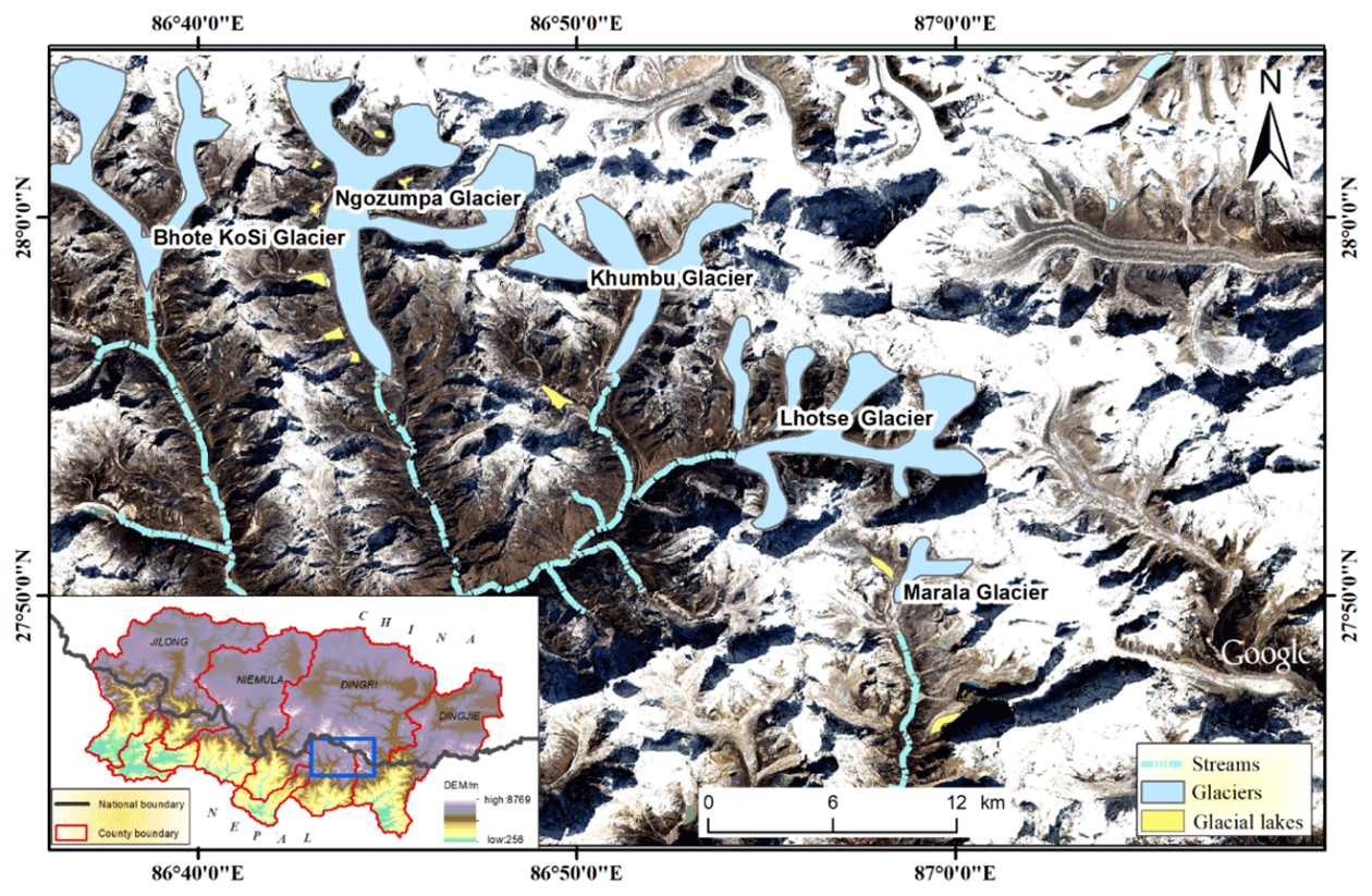
Figure 1 Location and topography information of the study area. All images © Google Earth 2020.

2.2 Data

2.2.1 Dataset and preprocessing

The global glacial lakes are mainly distributed in mountainous areas with many glaciers, including the Himalayas in Asia, the Buenos Aires mountains in South America (Bourgois et al., 2016), the Alaska mountains in North America (Rick et al., 2022), and the Alps in Europe (Huggel et al., 2002). Among them, Mount Qomolangma has different kinds of glacial lakes, such as the glacial erosion lake and the moraine-dammed lake, including seven types of glacial lakes according to the classification system summarized by Yao et al. (2017) (Fig. 2). Due to different development environments, the morphology of glacial lakes may differ in remote sensing images (Zhao et al., 2018). Collecting more samples of different types is of great help to enhance the stability and universality of the model (He et al., 2021). For the sake of increasing the diversity of the training dataset, except for the high-Asia region, this study also collected some glacial lake samples from other continents.

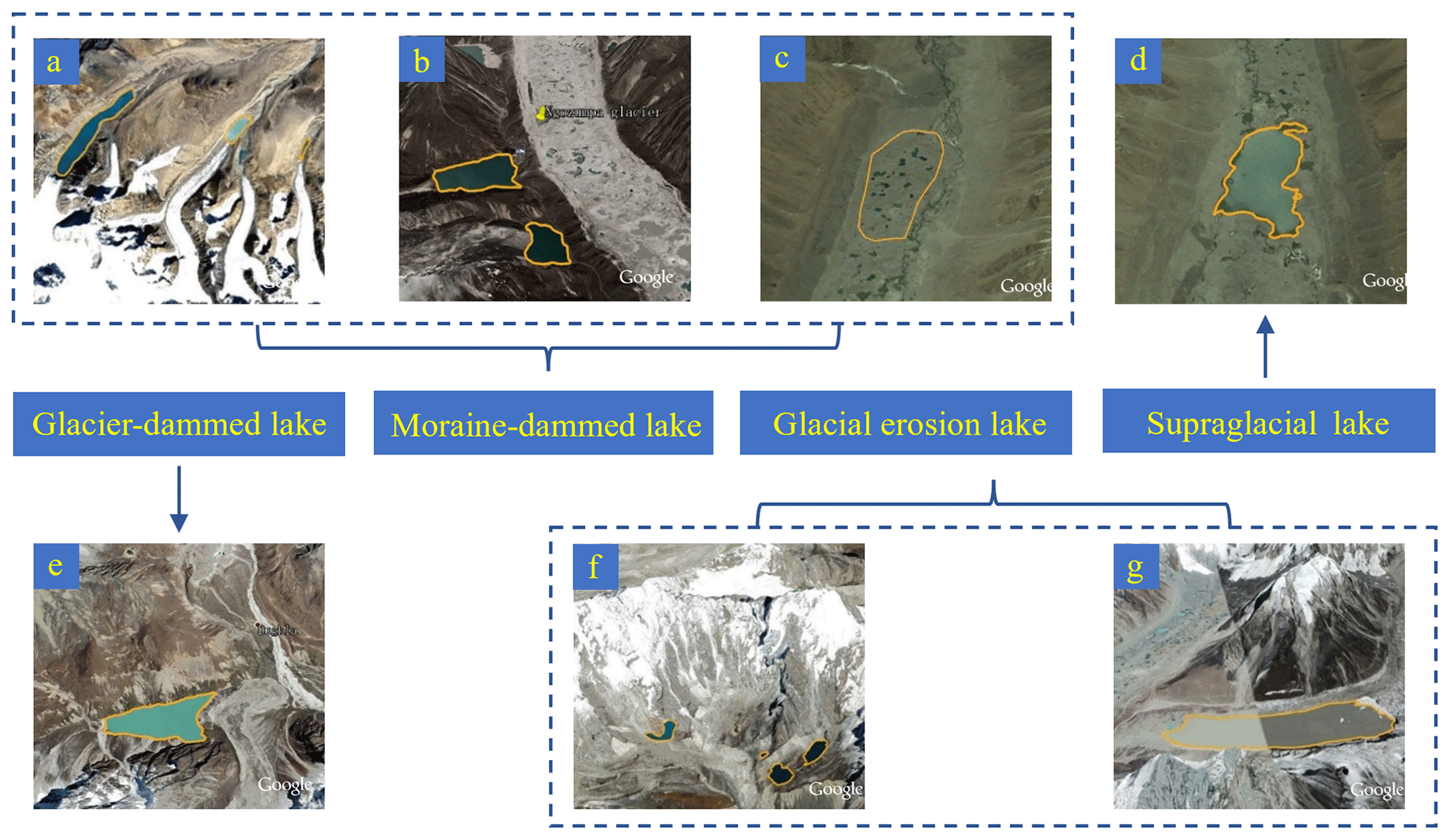
Figure 2 Seven types of glacial lakes in the training dataset. All images © Google Earth 2020. (a) Terminal moraine-dammed lake, (b) side moraine-dammed lake, (c) moraine thaw lake, (d) supraglacial lake, (e) glacial-dammed lake, (f) cirque lake, and (g) glacier valley lake.

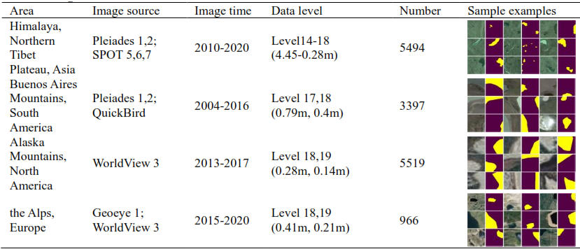
Google Earth imagery is a composite of a vast array of satellite and aerial photographs. These images are sourced from a variety of providers and platforms that are responsible for satellite launches. The primary contributors of high-resolution imagery include Maxar Technologies, the Centre National d'Etudes Spatiales (CNES), and Airbus. They provide IKONOS, QuickBird, GeoEye, WorldView, SPOT, and Pleiades imagery. Given that the sources of images vary across different regions, there is not a consistent time frame for image acquisition or a fixed spatial resolution. In Google Earth imagery, spatial resolution is categorized by levels – the higher the level, the greater the spatial resolution. In the data preprocessing, 14 to 19 levels of Google Earth images were chosen for the glacial lake dataset, and the image resolution covers the range of 5 to 0.14 m. When labeling, the glacial lakes were manually outlined with the help of ENVI 5.3 (other software, such as LabelMe and ArcGIS, can also do labeling), and every pixel in the image was labeled as 1 for glacial lakes or 0 for the background. When training the deep learning model, the images that were inputted into the network needed to be processed into image tiles for the limitation of the computer's memory capacity. After many experiments, it was more appropriate to divide the input images into non-overlapping image tiles of size 256×256. Image tiles that do not contain glacial lakes were removed to alleviate the problem of large background areas. Data augmentation operations were carried out to increase the number of samples, like image rotation. Finally, a total of 15 376 samples with a size of 256×256 were obtained, out of which 20 % of image tiles were selected as validation data randomly (Table 1).

Table 1 Details of the glacial lake training dataset based on Google Earth images in this study. All images © Google Earth 2020.

2.2.2 Other datasets

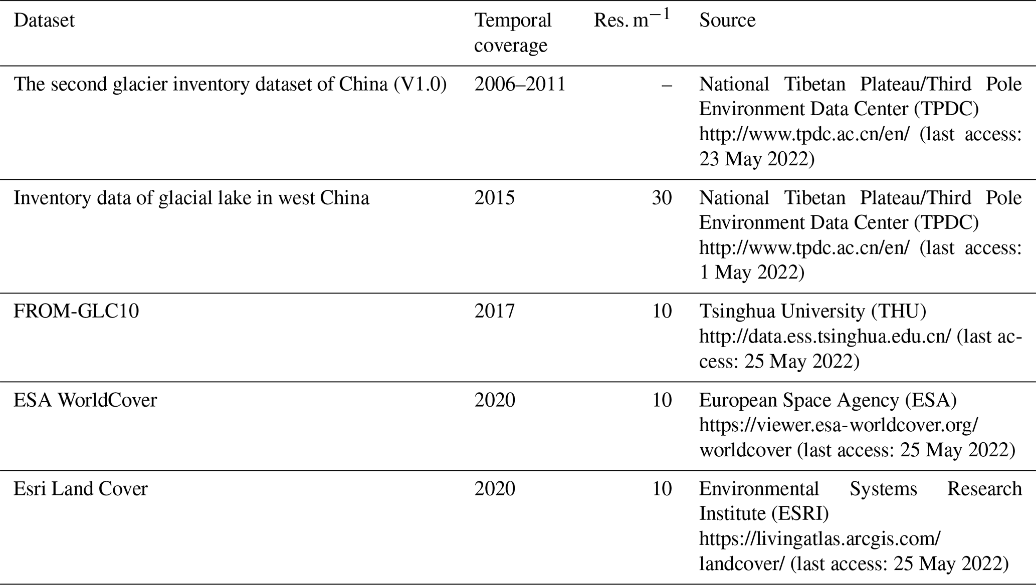
Except for the training dataset, other data products were also used to assist in completing this study (Table 2). The second glacier inventory dataset of China was used to delineate the distribution area of glacial lakes (Liu et al., 2012). In Sect. 4.3, the 30 m glacial lake inventory in western China based on Landsat TM/ETM+/OLI data (Wang, 2018) and three global land cover products (Gong et al., 2019) based on Sentinel-2 images were used for comparison with the glacial lakes extracted in this study.

Table 2 Other datasets used in this study.

3 Methods

In the glacial lake extraction method, based on Google Earth images, this study used the semantic segmentation framework to achieve rough extraction of the glacial lake first (“output1” in Fig. 3). In the pixel-based semantic segmentation, the outline of the glacial lake is not refined enough, which does not fit the actual smooth edge of the glacial lake. The simple linear iterative clustering (SLIC) algorithm could fuse the rough result of semantic segmentation with the edge information of superpixel segmentation to enhance the integrity of the glacial lake and improve the edge segmentation (“output2” in Fig. 3). The dense conditional random field (DenseCRF) uses the constraint relationship between pixels to encourage similar pixels to be assigned the same label, while pixels with large differences are assigned different labels to obtain accurate glacial lake outlines (“output3” in Fig. 3). In this paper, after semantic segmentation, two-level optimization combined SLIC and DenseCRF and was used to achieve refined extraction of glacial lake outlines. These two optimization methods can also be used separately to implement single-level optimization.

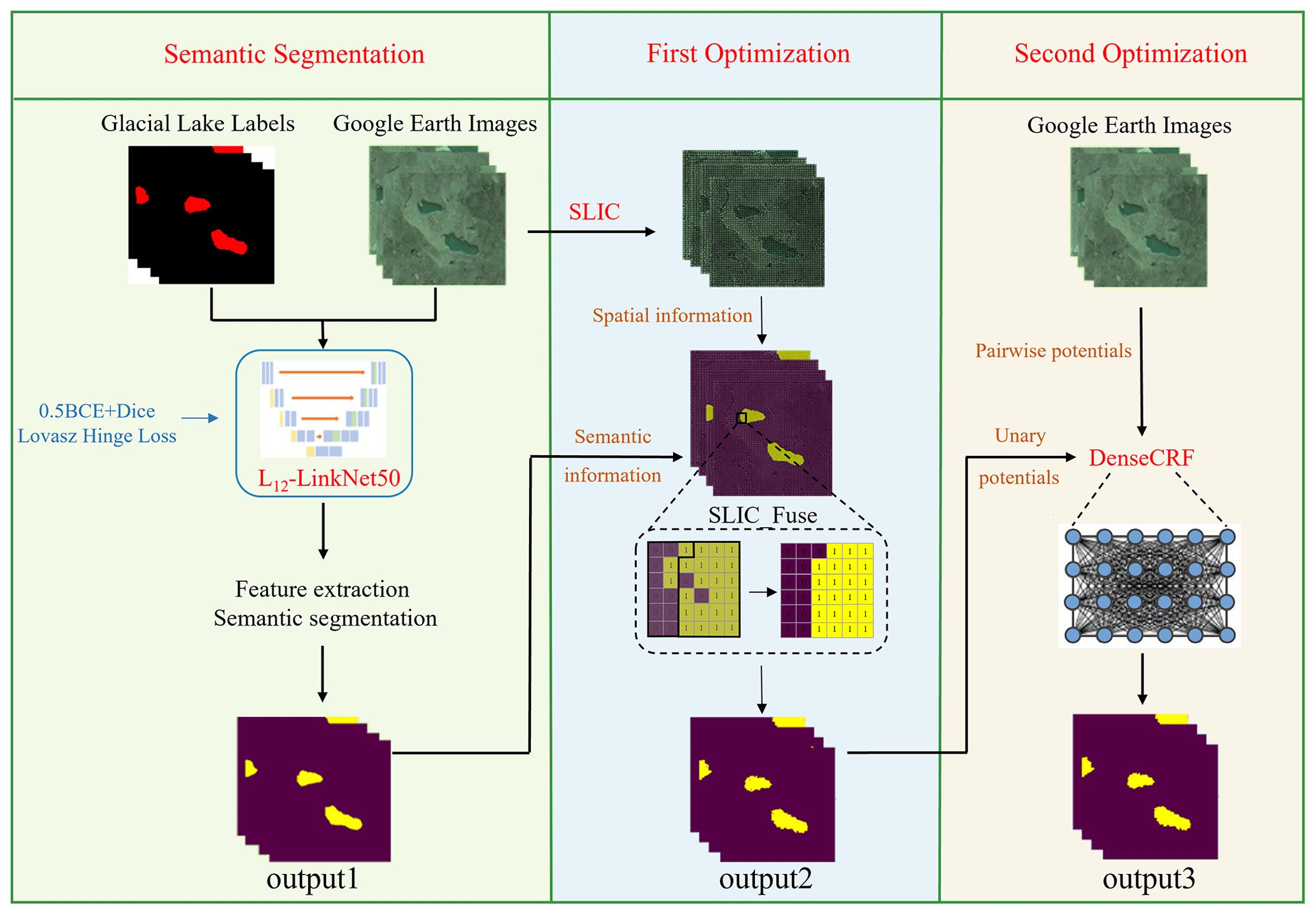
Figure 3 Structure diagram of glacial lake extraction strategy in this study. All images © Google Earth 2020.

3.1 Rough extraction of glacial lake information based on the semantic segmentation network

3.1.1 Deep residual network LinkNet50

The LinkNet network (Chaurasia and Culurciello, 2017) uses ResNet18 (He et al., 2016) as the backbone of the U-Net (Sathananthavathi and Indumathi, 2021). In the LinkNet network, the size of each layer feature map corresponding to encoder and decoder is the same, the addition method is used to combine the features, and the shallow features are re-learned without increasing the parameters, so that the spatial information of the glacial lake can be effectively restored, which has a lightweight structure and fast calculation speed. Good results have also been achieved in identifying glacial lakes, but the effect is unsatisfactory in areas covered with ice and snow or with a small number of glacial lakes. Moreover, high-resolution images in the dataset built in this study have complex spatial and spectral information, and deeper networks are more beneficial for high-level feature extraction (Li et al., 2020; Wang et al., 2021). Meanwhile, LinkNet50 has achieved good results in road detection based on high-resolution images (Li and Liu, 2022). Therefore, to obtain more useful features to distinguish glacial lakes from the background, this study used a deep residual network (ResNet50) instead of ResNet18 as the backbone of U-Net.

As shown in Table 3, ResNet of different depths contains five stages, and the output results (feature images) of the second to fifth stages are Res2, Res3, Res4, and Res5. In ResNet50, their sizes (width × height × channel) are $\mathrm{64}\times \mathrm{64}\times \mathrm{256}$, $\mathrm{32}\times \mathrm{32}\times \mathrm{512}$, $\mathrm{16}\times \mathrm{16}\times \mathrm{1024}$, and $\mathrm{8}\times \mathrm{8}\times \mathrm{2048}$, respectively. On the right side in Fig. 4, ResNet50 is used in the encoder of LinkNet50 for feature extraction to obtain high-level features. The input of each encoder layer is also bypassed to the output of the corresponding decoder layer. On the right side, the decoder uses the residual structure to combine low-level and high-level features and recover the detailed information of the image lost by the downsampling.

Table 3 The structure of ResNet of different network depths.

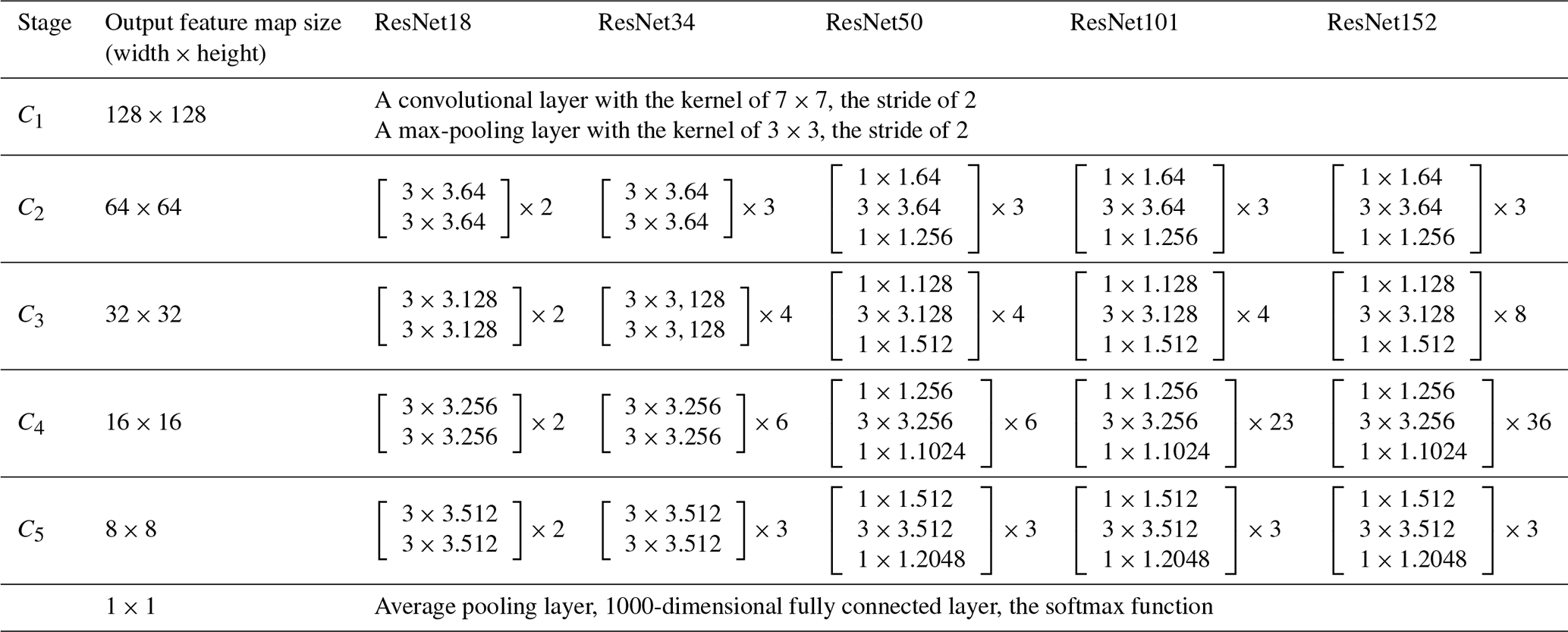
The size of the input image is $\mathrm{256}\times \mathrm{256}\times \mathrm{3}$. In the matrix multiplication expressions (five columns on the right), take ResNet18 as an example, where 3×3 indicates the convolution kernel size, 64 indicates the number of channels of the output image, and 2 indicates two residual blocks.

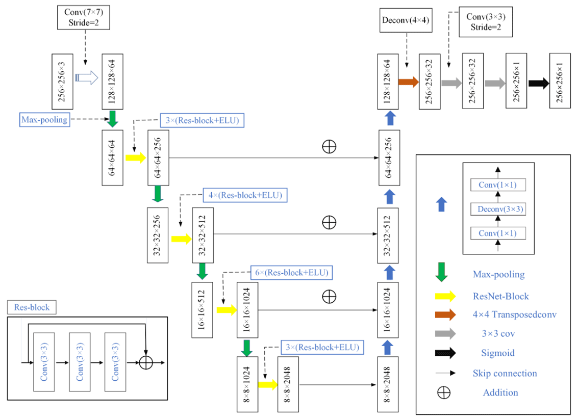
Figure 4 Schematic diagram of the LinkNet50 network structure used in this study. In the decoder, “conv” (1×1) is responsible for reducing the number of channels ($\times \mathrm{1}/\mathrm{4}$), and “deconv” (3×3) only changes the size of the feature map (×2). After the decoder, “transposedconv” (deconv (4×4)) reduces the number of channels ($\times \mathrm{1}/\mathrm{2}$) and expands the size of the feature map (×2).

3.1.2 Loss function

In the dataset in this study, the glacial lake area is small and the background area is large (unbalanced samples), so the target's features cannot be fully learned during the model training process. Therefore, to solve this problem, dice loss, which can help to reduce the impact of unbalanced positive and negative samples in binary classification, was used in this study. Dice loss essentially measures the overlap of two samples, and the calculation formula is

$$\begin{array}{}\text{(1)}& d=\mathrm{1}-\mathrm{2}\left|X\cap Y\right|/\left(\left|X\right|+\left|Y\right|\right),\end{array}$$

where |X| and |Y| indicates the number of pixels of sample X and sample Y, respectively, and |X∩Y| indicates the intersection of X and Y. For the common part that is repeatedly calculated, the coefficient of the |X∩Y| is 2.

However, dice loss will affect backpropagation, making the loss change unstable during model training. To increase the stability of the training process, BCE loss was introduced in this study. BCE loss belongs to the cross-entropy loss function, which is used to evaluate the difference between the probability distribution obtained by the training model and the natural distribution. In binary classification, the model predicted the probability of each category as p and 1−p, respectively, and the loss function is

$$\begin{array}{}\text{(2)}& \begin{array}{rl}L& ={\displaystyle \frac{\mathrm{1}}{N}}{\sum }_i{L}_i\\ & ={\displaystyle \frac{\mathrm{1}}{N}}{\sum }_i-\left[y_i\cdot \log \left(p_i\right)+(\mathrm{1}-y_i)\cdot \log (\mathrm{1}-p_i)\right],\end{array}\end{array}$$

where y_i is the label of sample i, 1 is for positive, and 0 is for negative. p_i is the probability that sample i is predicted to be positive. After testing, we finally adopted $\text{Loss1}=\mathrm{0.5}\text{BCE}+\text{Dice}$ as the loss function of the training model, which not only solved the problem of unbalanced positive and negative samples but also increased the stability of the network training process.

In addition, the Lovasz hinge loss is a convex Lovasz extension of submodular losses, which could optimize the IoU (intersection over union) loss of the network in the condition of unbalanced sample distribution (Berman et al., 2018). It is worth noting that the LinkNet50 with the Loss1 as the loss function is called L₁-LinkNet50 in this study. After L₁-LinkNet50, the Lovasz hinge loss (Loss2) was further used to fine-tune the deep semantic segmentation network in this study, which is referred to L₁₂-LinkNet50.

3.2 High-precision edge optimization algorithm

3.2.1 Simple linear iterative clustering (SLIC)

SLIC is a superpixel segmentation algorithm proposed by Achanta et al. (2012) with the advantages of a simple calculation process, high computation speed, and good edge matching. First, it converts the image from RGB to CIELAB, in which the five-dimensional vector V [l, a, b, x, y] consists of a $(l,a,b)$ color value and (x, y) coordinates of the corresponding pixel. Then based on the idea of K means, k superpixels are initialized in an image, and the distance between them is set as S. The core part is to iteratively calculate the centers of these superpixels by a clustering method. The distance for five-dimensional vectors (D^′) includes the distance of the CIELAB color space (d_c) and the geometric space (d_s). The following formulas are used to calculate the distance:

$$\begin{array}{}\text{(3)}& {\displaystyle }{d}_{\mathrm{c}}=\sqrt{(l_j-l_i{)}^{\mathrm{2}}+(a_j-a_i{)}^{\mathrm{2}}+(b_j-b_i{)}^{\mathrm{2}}},\text{(4)}& {\displaystyle }{d}_{\mathrm{s}}=\sqrt{(x_j-x_i{)}^{\mathrm{2}}+(y_j-y_i{)}^{\mathrm{2}}},\text{(5)}& {\displaystyle }{D}^{\prime }=\sqrt{(d_{\mathrm{c}}/m{)}^{\mathrm{2}}+(d_{\mathrm{s}}/s{)}^{\mathrm{2}}},\end{array}$$

where m indicates the maximum possible distance in the CIELAB color space and s indicates the maximum possible value in the geometric space.

For each superpixel center, the range of pixel searching is 2S×2S. If the distance from a pixel to the superpixel center i is less than the distance from it to the superpixel center to which it previously belonged, then this pixel is assigned to the superpixel i. In this iterative optimization algorithm, optimization persists until pixel distances to the new and previous superpixel centers stabilize. After iterating out the superpixel segmentation blocks of the image, the semantic segmentation results and SLIC segmentation are fused based on a rule. First, count the number of pixels with different semantic segmentation labels in a superpixel. Then the semantic label with more pixels is added to all pixels of this superpixel segmentation block.

3.2.2 DenseCRF

DenseCRF overcomes the limitation that CRF can only be performed in a local area and cannot connect full-text information (L. Zhang et al., 2018). The global context information of the whole image is organically combined, and all the pixels in the entire image are connected with the current pixel. DenseCRF is composed of unary potentials and pairwise potentials. Unary potentials come from the output of the front-end semantic segmentation network, which refers to the potential of predicting the pixel point (i) as a semantic label (x_i) through the semantic segmentation network. Pairwise potentials describe the relationship of each pixel to all other pixels in the image, mainly providing position and spectral information through the original input image (Berman et al., 2018). Therefore, it not only makes predictions for a single pixel but also calculates the probability of different classes appearing simultaneously.

3.3 Accuracy assessment indicators

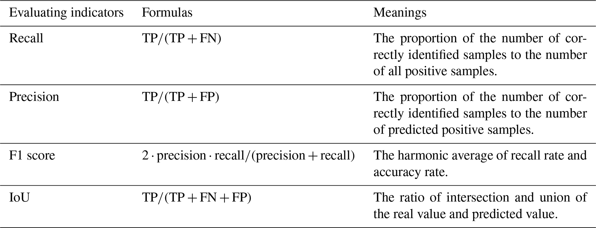
Scientific selection of evaluation indicators is the key to testing the accuracy of glacial lake extraction results. Four indicators – recall, precision, F1 score (Yacouby and Axman, 2020), and IoU (Rahman and Wang, 2016) – were selected as the indicators for the accuracy evaluation of glacial lake extraction results. And all of them are generated based on the true positive (TP), true negative (TN), false positive (FP), and false negative (FN).

Table 4 Meanings and calculation formulas of four evaluation indicators.

4 Experiments and results

Based on high-resolution Google Earth images (level 18, with an image resolution of 0.52 m) in the study area, we used L₁-LinkNet50 for the preliminary extraction in the rough extraction stage. The commonly used semantic segmentation models (U-Net, LinkNet) and traditional machine learning methods (SVM and RF) were chosen for comparison. Moreover, among the improved semantic segmentation methods for glacial lakes, EfficientNet U-Net (Qayyum et al., 2020) was proposed based on high-resolution images (3–4 m) and was also chosen for comparison. Our experiment was based on Python 3.6 and the open-source deep learning framework PyTorch. In the SVM classifier, the penalty coefficient (C) was set to 12, the kernel was set to the radial basis function (rbf), and the gamma in the kernel function was set to 0.187. In the RF classifier, the number of decision trees was set to 150, and the number of features is set to 2. The training was performed on an NVIDIA GeForce RTX 2080 Ti, using cuDNN10.0 for acceleration. The batch size was set to 4. For the semantic segmentation network, the optimization method adopted the Adaptive Moment Estimation (Adam), and the initial learning rate was set to $\mathrm{1}\times {\mathrm{10}}^{-\mathrm{4}}$. Moreover, the learning rate update strategy of polynomial decay was adopted to prevent the network from sinking into local optimal solutions later in model training, in which the momentum and weight decay were set at 0.9 and $\mathrm{1}\times {\mathrm{10}}^{-\mathrm{4}}$, respectively. This study trained all networks for 45 epochs in this stage.

4.1 Comparative analysis of rough extraction results

Recall, precision, F1 score, and IoU were calculated to evaluate the extraction results against the ground truth obtained by manual digitization. As can be seen in Fig. 5, the edges of the glacial lakes extracted by SVM and RF are rough. There are difficulties in the complete extraction of complex glacial lakes and small glacial lakes, which affects the recall. In deep learning models, the U-Net network is greatly affected by snow (Fig. 5e), and the probability of being wrongly classified as glacial lakes is high, which decreases the precision and F1 score. EfficientNet U-Net obtains the highest precision, and the predicted water masks have few false positives, which is consistent with the conclusions of Qayyum et al. (2020). This method reduced false detections of glacial lakes in snow-covered areas compared to U-Net (Fig. 5e). However, there are still problems for glacial lakes with similar spectral information to the background and for glacial lakes that are shaded by mountain shadows. LinkNet can identify more glacial lakes than EfficientNet U-Net. But some false detections are prone to occur in the shaded area (Fig. 5c), and the precision is reduced. Finally, after introducing the deep residual network, L₁-LinkNet50 improved the extraction of glacial lakes with small areas and glacial lakes shaded by mountain shadows. Although the precision is slightly lower than that of EfficientNet U-Net, the final F1 score of L₁-LinkNet50 reaches 87.77 % and the recall is 3.46 % higher than that of EfficientNet U-Net (Table 5). Therefore, it can be found that L₁-LinkNet50 has the most vital comprehensive ability for glacial lake extraction in these models.

Table 5 Quantitative evaluation for glacial lake extraction.

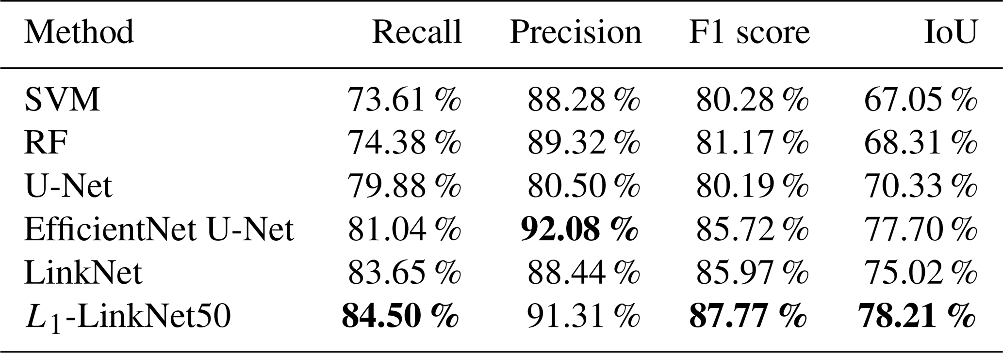
The bold font represents the highest score.

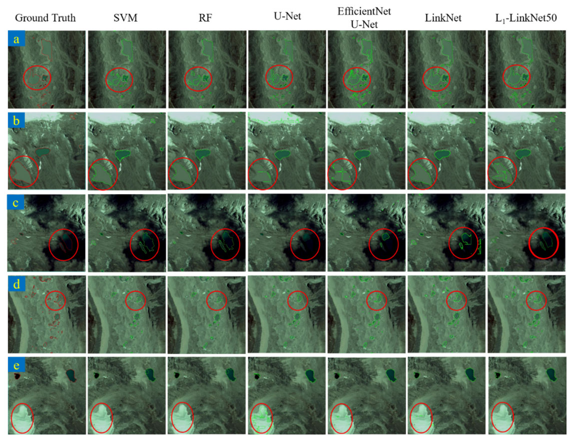
Figure 5 Performance comparison of different models for the glacial lake extraction. All images © Google Earth 2020. Five regions of the same size (2048×2048) were chosen based on Google Earth images (0.52 m). The red shapes are the boundary of the ground truth glacial lakes, and the green shapes are the boundary of the predicting results, including areas with glacial lakes of complex outlines (a), the inconsistent color of water bodies (b), mountain shadows (c), and areas with multiple small glacial lakes (d) and ice and snow (e).

4.2 Comparative analysis of optimization results

L₁-LinkNet50 showed the best effect to extract glacial lakes in Sect. 4.1. This study improved L₁-LinkNet50 and carried out post-processing on the glacial lake segmentation results. L₁-LinkNet50 was trained for another 25 epochs for L₁₂-LinkNet50, using the Lovasz hinge loss (Loss2) as the loss function. Then the two-level optimization strategy (SLIC and DenseCRF) was used to optimize semantic segmentation results. For superpixel segmentation, the number of superpixels, compactness, and iteration times were set as 2800, 60, and 10, respectively. Then the semantic segmentation result by L₁₂-LinkNet50 or the fusion result by SLIC and L₁₂-LinkNet50 was input into DenseCRF as the unary potential. In this process, the mean-field approximation method was used for inference to minimize the potential function.

In Table 6, after L₁-LinkNet50 was trained with the Lovasz hinge loss, the IoU reached 83.77 % in the study area, which was 5.56 % higher than that of L₁-LinkNet50. It alleviated the problems of adhesions (multiple glacial lakes nearby detected as one) (Fig. 6 (3) and (4)) and missed detections (Fig. 6 (2)). In addition, it is difficult for the semantic segmentation network to recover all the lost spatial information when upsampling, resulting in imprecise segmentation edges. The glacial lakes after superpixel segmentation optimization are closer to the natural boundary, especially the small glacial lakes. Post-processed results by DenseCRF had smoother edges, and the precision increased by 0.86 %. Moreover, after using two-level optimization (SLIC–DenseCRF), missed detections of glacial lakes were effectively reduced. Compared to L₁₂-LinkNet50, the IoU and F1 score increased by 6.92 % and 3.96 %, respectively. The comparison of results based on different optimization algorithms proves that the post-processing based on SLIC–DenseCRF for deep learning semantic segmentation results can improve the accuracy of glacial lake extraction.

Table 6 Evaluation indicators for glacial lake identification results under different optimization conditions.

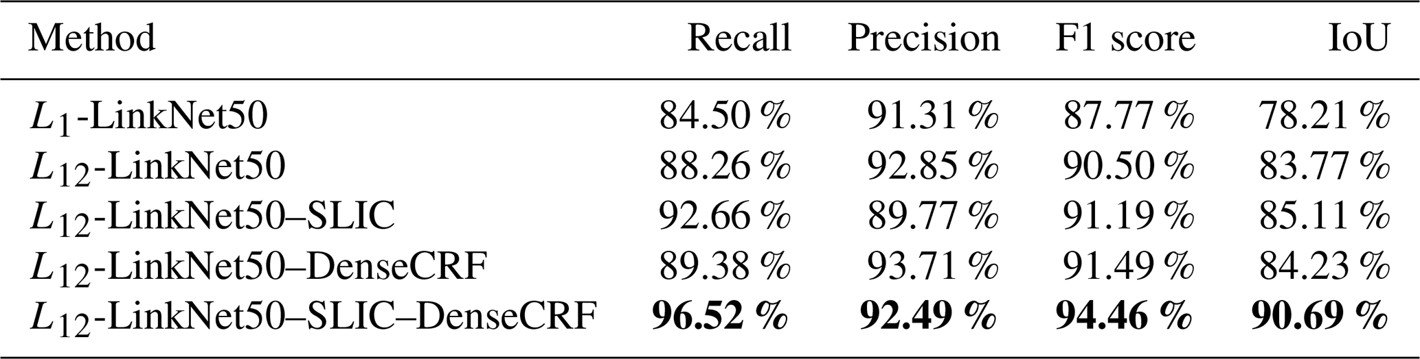
The bold font represents the highest score.

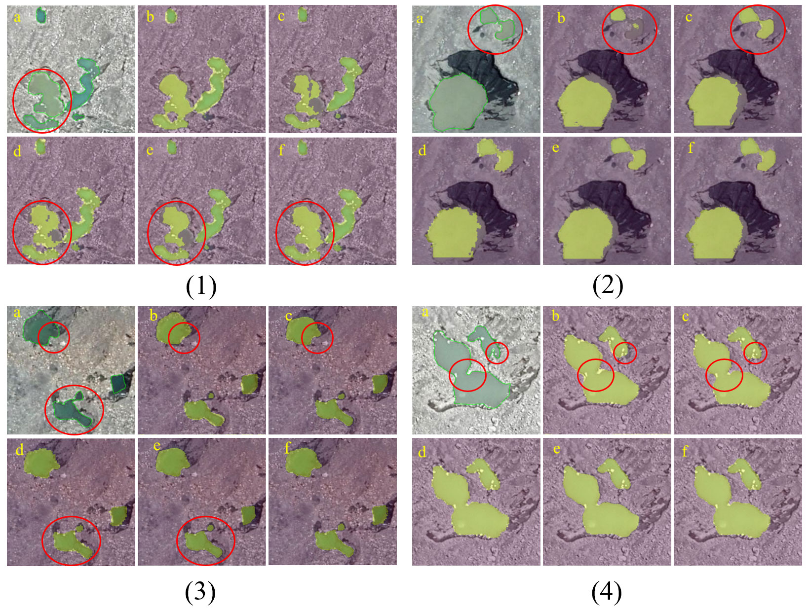
Figure 6 Comparison of glacial lake identification results based on Google Earth images (0.52 m) under different optimization conditions. All images © Google Earth 2020. Ground truth (a), L₁-LinkNet50 (b), L₁₂-LinkNet50 (c), L₁₂-LinkNet50–SLIC (d), L₁₂-LinkNet50–DenseCRF (e), and L₁₂-LinkNet50–SLIC–DenseCRF (f). The green shapes are the boundary of the ground truth glacial lakes, and the yellow masks are the predicting results.

4.3 Glacial lake extraction in Qomolangma National Nature Reserve

After evaluating the ability of the glacial lake extraction method proposed in this study, we applied L₁₂-LinkNet50–SLIC–DenseCRF to the extraction of glacial lakes in the Qomolangma National Nature Reserve (QNNR). This reserve has a total area of 33 819 km², including the core area, the buffer area, and the experimental area. Because it is difficult to obtain the sub-meter-level Google Earth image of the entire QNNR, Google Earth images (level 16) in 2020 within the 10 km buffer zone from the end of the glacier in QNNR were used as the data source, with an image resolution of 2.11 m. For the glacial lake extraction in QNNR, the evaluation results show that the precision, F1 score, recall, and IoU are 85.55 %, 82.49 %, 79.65 %, and 70.20 %, respectively. The IoU of the actual application is lower than the rectangular study area, but the precision has reached more than 85 %. The final result is shown in Fig. 7. In the QNNR, glacier lakes are mainly distributed in the altitude range of 4000 to 6000 m. The area and number of glacial lakes are approximately normally distributed, and both peak at 5000–5500 m, which is consistent with the research of Yang et al. (2019) and Zhang et al. (2021). The area and number of glacial lakes at the peak account for 66.58 % and 39.70 % of all glacial lakes, respectively.

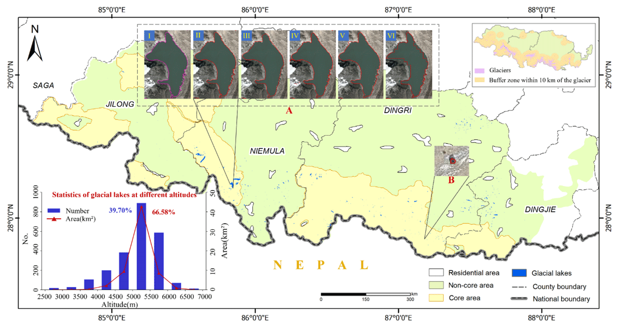
Figure 7 Glacial lake extraction result in the QNNR based on Google Earth images in 2020 (2.11 m). All images © Google Earth 2020. A and B are the largest and smallest glacial lakes extracted in this region, respectively. The purple shapes are the boundary of the ground truth glacial lakes, and the red shapes are the boundary of the predicting results. Ground truth (I), L₁₂-LinkNet50–SLIC–DenseCRF 2.11 m (II), inventory data of glacial lake 30 m (III), ESA WorldCover 10 m (IV), Esri Land Cover 10 m (V), and FROM-GLC10 10 m (VI).

Compared with the existing glacial lake inventory and three land cover datasets in Sect. 2.2.2, the glacial lakes extracted based on the proposed method are closer to the ground truth in terms of the number and area (Fig. 8a). The area of the largest glacial lake (5.943 km²) of the reserve extracted in this study is consistent with the other four and is closest to the ground truth. For glacial lakes with an area greater than 0.01 km², the distribution of the number of glacial lakes is similar for all datasets. However, for small glacial lakes, due to the advantages of remote sensing image sources and methods, the accuracy of the extraction results of glacial lakes in this study is significantly better than the other four existing datasets. Moreover, we checked the results of the glacial lake extraction in the QNNR and found that the smallest glacial lake that can be fully and correctly extracted has an area of 160 m².

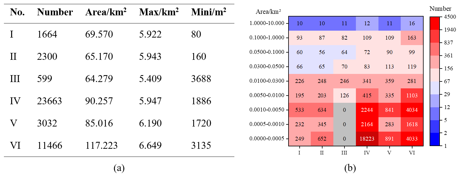
Figure 8 Comparison of glacial lakes between this study and the other four datasets. Basic information (a) and statistical information on the number distribution of glacial lakes in different areas (b). Ground truth (I), L₁₂-LinkNet50–SLIC–DenseCRF 2.11 m (II), inventory data of glacial lake 30 m (III), ESA WorldCover 10 m (IV), Esri Land Cover 10 m (V), and FROM-GLC10 10 m (VI).

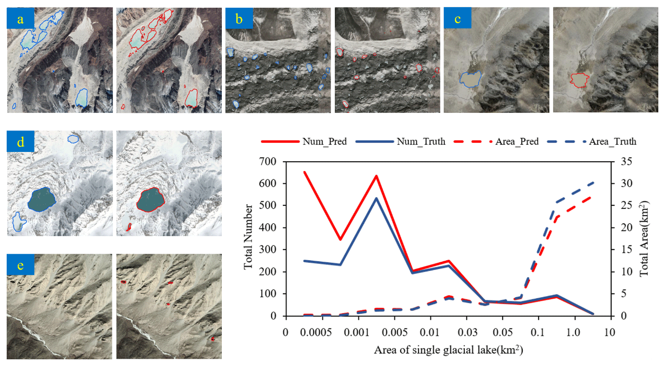
Figure 9 The display of glacial lake extraction results in different situations in the QNNR, as well as the statistics of area and number. All images © Google Earth 2020. The blue shapes are the boundary of the ground truth glacial lakes, and the red shapes are the boundary of the predicting results.

5 Discussion

The lack of reliable glacial lake samples is one of the difficulties in the development of glacial lake extraction research based on deep learning networks (J. Wang et al., 2022). Qayyum et al. (2020) also stated that because of insufficient types of glacial lakes in the training dataset, some muddy brown glacial lakes could not be identified. The high-resolution samples built in this study help to improve the evaluation indicators. Moreover, L₁₂-LinkNet50 uses a deep residual structure (ResNet50) as the backbone of the network, which enhances the ability to extract glacial lakes under different background conditions and is also better at the boundary of the small glacial lake (Fig. 9b). Therefore, compared with other methods as shown in Sect. 4.1, the evaluation indicators of glacial lakes extracted by L₁₂₋LinkNet50 are improved. The proposed method in this study can effectively reduce missed detections of some glacial lakes that show similar spectral features with soil (Fig. 9c) and shadows.

For post-processing, the parameter values used in the SLIC algorithm in this study, including the number of superpixel blocks (2800) and the compactness (60), were obtained through multiple experiments by the control variable method based on sub-meter-level images. When the image resolution differs greatly, the amount of semantic information in a single superpixel will change. Thus, these parameter values are not applicable to images with a spatial resolution of 10 m such as band 2, 3, and 4 of Sentinel images. In addition, frozen lakes generally start from the edge with shallow water bodies and more small rocks, resulting in more noise on the edge of glacial lakes. DenseCRF connects the local and global information to set up pairwise potentials on all pairs of pixels, providing more detailed labeling and reducing the small-area noise generated by the image segmentation of high-resolution images. As a result, the optimized glacial lakes have smoother edges (Fig. 9a) and fewer false spots on the lake surface.

For the glacial lake extraction results of the QNNR, the curve in Fig. 9 shows that the area distribution of small-area glacial lakes is consistent with the results of manual digitization. However, although the proposed method is effective in identifying glacial lakes with similar spectral information to shadows, it is prone to misjudge in small areas of shadows (Fig. 9e). Because the area of these shadows is too small, little spectral and texture information on the background can be extracted, so it is difficult to distinguish by the method in this study. The number distribution of large-scale glacial lakes is consistent with the results of manual digitization, but more large-area glacial lakes have not been fully identified. The spectral information of glacial lakes completely covered by snow and some glacial lakes that have been frozen for a long time is very similar to that of snow. At present, the proposed method in this study cannot fully identify those glacial lakes (Fig. 9d). In the Google images captured over the QNNR area, large areas of the land were covered with snow. This is also the reason why glacial lake evaluation indicators of the QNNR are lower than those of the small study area in Sect. 4.2.

6 Conclusions

Aiming at the demand for high-accuracy outline extraction of glacial lakes in the high-Asia region, this study built a dataset for glacial lakes based on the global meter-level to sub-meter-level Google Earth images and then proposed the glacial lake extraction method of the L₁₂-LinkNet50 semantic segmentation network with two-level optimization of SLIC–DenseCRF.

Based on the dataset containing glacial lakes of multiple types, the ability to identify glacial lakes of different types and colors is improved in this study. The Lovasz hinge loss and 0.5 BCE + dice are combined to improve the loss function of the deep semantic segmentation network and suppress the impact of the unbalanced positive and negative samples in the dataset. It has the advantage of small glacial lake detection and effectively reduces the missed detection of glacial lakes that have similar spectral features to the bare soil or shadows. The F1 score in the study area reaches more than 90 %. At the same time, it is applied to a wider range of QNNR. Due to the misjudgment of the small glacial lake in the shadow, the F1 score is reduced, but it also reaches 82.49 %. By post-processing for the semantic segmentation results, the edges of glacial lakes are more consistent with the actual situation, and the noise spots on the lake surface are also reduced.

Although the proposed method has achieved good extraction results on the new dataset, there are still shortcomings in the recognition of snow-covered glacial lakes and terrain shadows with small areas. For future research, multi-source remote sensing images can be used to reduce the impact of snow cover and shadows.