the Creative Commons Attribution 4.0 License.
the Creative Commons Attribution 4.0 License.
 | 05 Apr 2024
The influence of glacial landscape evolution on Scandinavian ice-sheet dynamics and dimensions
Gustav Jungdal-Olesen
Jane Lund Andersen
Andreas Born
Vivi Kathrine Pedersen
The Scandinavian topography and bathymetry have been shaped by ice through numerous glacial cycles in the Quaternary. In this study, we investigate how the changing morphology has influenced the Scandinavian ice sheet (SIS) in return. We use a higher-order ice-sheet model to simulate the SIS through a glacial period on three different topographies, representing different stages of glacial landscape evolution in the Quaternary. By forcing the three experiments with the same climate conditions, we isolate the effects of a changing landscape morphology on the evolution and dynamics of the ice sheet. We find that early Quaternary glaciations in Scandinavia were limited in extent and volume by the pre-glacial bathymetry until glacial deposits filled depressions in the North Sea and built out the Norwegian shelf. From middle–late Quaternary (∼0.5 Ma) the bathymetry was sufficiently filled to allow for a faster southward expansion of the ice sheet causing a relative increase in ice-sheet volume and extent. Furthermore, we show that the formation of The Norwegian Channel during recent glacial periods restricted southward ice-sheet expansion, only allowing for the ice sheet to advance into the southern North Sea close to glacial maxima. Finally, our experiments indicate that different stretches of The Norwegian Channel may have formed in distinct stages during glacial periods since ∼0.5 Ma. These results highlight the importance of accounting for changes in landscape morphology through time when inferring ice-sheet history from ice-volume proxies and when interpreting climate variability from past ice-sheet extents.
- Article
(12969 KB) - Full-text XML
- BibTeX
- EndNote


Ice holds the power to transform landscapes and constituted a major geomorphological agent in northern Europe during the Quaternary (last 2.6 Ma) where recurring glacial cycles shaped the present-day landscape. Indeed, the topography and bathymetry in and around northern Europe reveal the extensive impact of its rich glacial history, with deep fjords and U-shaped valleys attesting to the accumulated effect of widespread glacial erosion and terminal moraines indicating the extent of past ice sheets (Hughes et al., 2016; Stroeven at al., 2016). The Eurasian ice-sheet complex covered much of the British Isles, all of Scandinavia, and much of northern Europe including parts of Germany, Poland, Russia, and the Baltic through multiple glacial cycles since 1 Ma (Batchelor et al., 2019). During the Last Glacial Maximum (LGM), the ice-sheet complex, consisting of the Scandinavian ice sheet (SIS), the Barents Sea ice sheet (BSIS), and the British–Irish ice sheet (BIIS), contained an ice volume corresponding to m sea-level equivalent (Simms et al., 2019). On a global scale, the pace of these glacial cycles results from solar insulation variations combined with feedback mechanisms and internal dynamic effects in the climate system, in part caused by the ice sheets themselves (Hughes and Gibbard, 2018). Differences in both ice volume and the extent of ice sheets between glacial cycles (Fig. 1) can also be attributed to variations in moisture supply through complex global atmosphere–ocean–ice interactions (e.g., Batchelor et al., 2019; Hughes and Gibbard, 2018), with topography and proximity to the ocean being key factors determining the spatial distribution of moisture to an ice sheet. Studies on glacial landscape evolution have indicated that glacial erosion and deposition can also influence ice-sheet dynamics as well as ice volumes and extent (e.g., Kessler et al., 2008; Kaplan et al., 2009; MacGregor et al., 2009; Egholm et al., 2009, 2012a, b, 2017; Anderson et al., 2012; Pedersen and Egholm, 2013; Pedersen et al., 2014; Clague et al., 2020; Mas e Braga et al., 2023). But until now, these studies have been limited to synthetic landscapes and/or limited spatial scales (smaller glaciers and ice caps). A few ice-sheet scale models are starting to consider glacial erosion (e.g., Patton et al., 2022), but the effects of long-term Quaternary landscape evolution on ice-sheet dynamics are still to be explored on a large scale for realistic landscapes and ice-sheet configurations. Understanding the influence of landscape evolution on ice-sheet dynamics requires the reconstruction of landscapes that existed prior to or at earlier stages of glacial erosion, something that can be approached using source-to-sink studies, utilizing offshore sediment volumes of a glacial origin (e.g., Steer et al., 2012; Paxman et al., 2019; Pedersen et al., 2021).
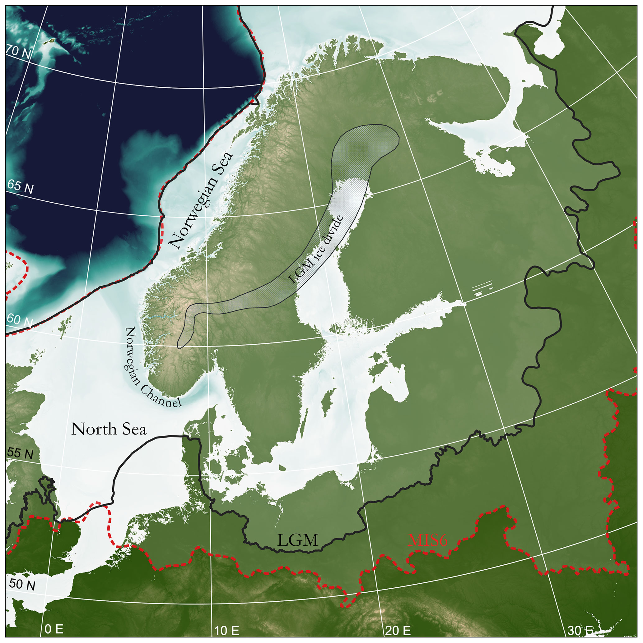
Figure 1Overview map of the model domain. The maximum plausible extent of the Fennoscandian ice-sheet complex during the Last Glacial Maximum (LGM; black line) and the Penultimate Glacial Maximum (MIS 6; dashed red line) are overlaid (Batchelor et al., 2019). Also shown is the approximate location of the LGM ice-divide position (Olsen et al., 2013).
In this work, we focus on the well-studied Scandinavian region and investigate how the SIS may have changed its behavior because of Quaternary landscape evolution. We use a higher-order ice-sheet model to investigate how large-scale glacial morphological features have influenced the development and dynamics of the SIS over a glacial cycle at two key times during the Quaternary: (1) before the inception of major glaciations in the beginning of the Quaternary (PREQ ∼2.6 Ma) and (2) during the middle–late Quaternary (MLQ ∼0.5 Ma) where major pre-glacial features in the bathymetry around Scandinavia had been filled with glacial deposits (Dowdeswell and Ottesen, 2013). Importantly, we do not intend to reconstruct realistic SIS configurations for these past time periods, but rather keep the climate forcing consistent between experiments, in order to isolate how changes in bed morphology has impacted SIS dynamics and extent. This allows us to (i) explore how morphological changes can influence the dynamics, extent, and volume of the ice sheet, independent of the climatic forcing, and (ii) gain insight into how ice-volume proxies could be influenced by glacial landscape evolution.
For the early Quaternary, we adopt the pre-glacial landscape reconstructions provided for the Scandinavian region by Pedersen et al. (2021) that include (i) the absence of glacially generated sediments offshore, (ii) infill of over-deepened fjords and glacial valleys onshore, (iii) a reconstructed wedge of older Mesozoic and Cenozoic sediments on the inner shelf that is assumed to have been eroded by glacial activity within the Quaternary (e.g., Hall et al., 2013), and finally, (iv) adjustments of the landscape owing to erosion- and deposition-driven isostatic changes and dynamic topography (Pedersen et al., 2016).
In addition to this pre-glacial reconstruction, which explores an entirely different offshore bathymetry and onshore Scandinavian landscape, we also consider the more subtle effects of the large glacial troughs that have been carved into the shelf bathymetry by ice streams since the middle–late Quaternary. One of the most notable of these glacio-morphological features offshore Scandinavia is The Norwegian Channel (Fig. 1). This channel is believed to have been formed by ice-stream activity sometime since 1.1 Ma (e.g., Sejrup et al., 2003), with studies suggesting that ∼90 % of the deposits funneled through the channel and into the North Sea Fan were deposited within the last ∼0.5 Ma (Hjelstuen et al., 2012). Recently, it has been argued that the channel formed before ∼0.35 Ma (Løseth et al., 2022). An erosional unconformity at the base of the channel is draped by post-LGM sediments, suggesting that the channel experienced erosion within the last glacial cycle (Hjelstuen et al., 2012).
For the numerical experiments presented in this study, we use the depth-integrated second-order shallow-ice approximation iSOSIA (Egholm et al., 2011, 2012a, b). We conduct our experiments by simulating a full glacial cycle of 120 ka on different topographies. In the following section we will present the numerical model, the model setup, and the experimental design.
2.1 Modeling the Scandinavian ice sheet
The ice flow in iSOSIA is governed by a second-order approximation of the equations for Stokes flow (e.g., Egholm et al., 2011). The velocities are depth integrated to yield a 2D one-layer ice model, implemented here using a regular grid (e.g., Egholm and Nielsen, 2010). The second-order nature of the approximation ensures that ice velocities depend non-linearly on ice thickness, ice-surface gradients, as well as longitudinal and transversal horizontal stress gradients (Egholm et al., 2011, 2012b). Details on the iSOSIA model, including the importance of the higher-order ice dynamics involved, have been described in depth elsewhere (Egholm and Nielsen, 2010; Egholm et al., 2011, 2012a, b).
The depth-integrated ice-creep velocity is calculated using temperature-dependent Glen's flow with a stress exponent, n, equal to 3:
where is the strain rate tensor, ij denotes the components of the tensor, Aflow is the ice flow parameter, τe is the effective stress, and s is the deviatoric stress tensor (Egholm et al., 2011). The ice flow parameter Aflow is dependent on the depth-averaged temperature of the ice using an exponential relationship:
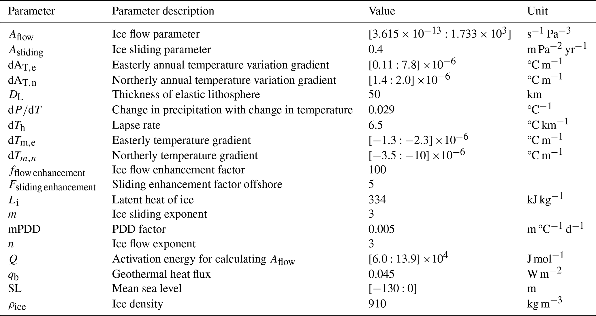
where A0 is a flow constant, Q is an activation energy, R is the gas constant, and T is the temperature relative to the pressure melting point (e.g., Zeitz et al., 2020). A0 and Q have different values above and below °C (see Table 1). A simple Weertman sliding scheme is used to calculate the contribution of basal sliding to depth-integrated ice velocities:
where ub is the basal velocity, Asliding is an ice sliding coefficient, ts is the bed-parallel shear stress, and N is the effective pressure at the base (Egholm et al., 2011). Asliding is chosen to give realistic sliding in the order of several hundred meters per year, for example, in fjords or near the shelf edge in the Norwegian Sea, similar to surface velocities in comparable areas of modern-day ice bodies (e.g., Millan et al., 2022). To allow for faster ice flow for soft-bed subglacial conditions (e.g., Gladstone et al., 2020; Han et al., 2021), Asliding is enhanced by a factor of 5 in offshore regions and onshore in northern Europe where thick, soft sediments cover the bed.
In this study, we focus on grounded ice only, as ice-shelf dynamics are computationally expensive to resolve on the timescales of our experiment and because constraints on ice-shelf extent in middle or early Quaternary glaciations are sparse due to a lack of reliable dates on submarine landforms (e.g., Jakobsson et al., 2016). Some older studies suggest that an ice shelf was present during recent glaciations in the North Atlantic and Arctic regions (Hughes et al., 1977; Lindstrom et al., 1986). However, while ice-shelf stability is sensitive to bathymetric configurations (Bart et al. 2016) and is a deciding factor in grounding line migration, we limit our focus here to large-scale morphological features, such as the Norwegian Channel, created by an ice stream in contact with the seabed (Sejrup et al., 2016). Consequently, we do not consider floating ice in our simulations and remove floating ice by introducing a fast melt rate for ice that does not meet the grounding criterion:
where Hice is ice thickness, SL is local sea level, and ρwater and ρice are the densities of water and ice, respectively. Mean sea level in the model is varied between the interglacial and glacial maximum (−130 m) using the normalized LR04 Benthic Stack (Lisiecki and Raymo, 2005) as a glacial index. Special boundary conditions are employed at the approximate locations where the SIS meets the BSIS and BIIS by introducing an “ice wall” where the ice flux is zero to emulate divergent ice flow when these ice sheets merge during glacial maxima. At the edges of the model domain, we employ open boundary conditions to allow ice to flow out of the domain. Common model parameters are presented in Table 1.
Table 1Common parameters in the ice-sheet model and mass balance scheme. Numbers in brackets denote minimum and maximum values.
2.1.1 Mass balance
In the simulations we present here, we assume that the mass balance () of the ice sheet can be approximated using three components:
where is the rate of accumulation, is the surface melt rate, and is the basal melt rate (Egholm et al., 2012b). We use a positive-degree-day (PDD) model to estimate accumulation rate and surface melt rate as a function of mean annual temperature, annual temperature variation, and mean annual precipitation at every point in our model domain for every time step (e.g., Magrani et al., 2022).
The yearly temperature variation in each cell is approximated by a sine function based on the mean annual temperature and annual temperature amplitude (see below). The melt rate (in m yr−1) is calculated in the PDD model as
where mPDD is the positive-degree-day factor multiplied by the sum of positive degrees Tpositive each year. Here, we consider a single melting degree factor for both ice and snow since all precipitation is turned into ice after accumulation (based on yearly average rates). The accumulation rate is approximated by
where nfrost is the number of days with negative temperatures in a year and P is the annual precipitation. The temperature forcing that drives spatial and temporal changes in mass balance in our simulations is based on mean temperature, annual temperature amplitude, and lapse rate, all of which vary across the model domain using spatial gradients that vary in time. Two climate states, a glacial maximum state and an interglacial state, are chosen to represent the extremes of our model, and the spatial gradients of the full glacial cycle of our model simulations are subsequently defined to vary in between these extremes using a glacial index that resembles the normalized LR04 Benthic Stack (Lisiecki and Raymo, 2005) with the glacial maximum in this climate forcing occurring at 18 ka BP. Here, we define spatial (x, y, z) gradients at the glacial maximum using multiple linear regression on MPI-ESM climate model outputs (LGM experiment; Jungclaus et al., 2019). For the interglacial state we define spatial gradients using the ERA-Interim reanalysis data for modern day (Dee and National Center for Atmospheric Research Staff, 2022). Finally, the lapse rate was found to be close to constant, so we keep this fixed at 6.5 °C km−1. With this approach, the temporally varying temperature forcing of the entire grid can be defined from a single grid cell in the lower left corner while still capturing a coastal–continental (east–west) gradient, a polar gradient (south–north), and an altitudinal gradient (lapse rate) in temperature. However, we cannot capture local effects that arise from changes in complex atmospheric circulations patterns over time that might have important implications for glacial dynamics and ice extent (e.g., Liakka et al., 2016; Hughes and Gibbard, 2018).
To represent precipitation in our simulations, we use a climate-corrected modern-day mean precipitation field (Pendergrass et al., 2022), modulating the local precipitation in every grid cell using the following equation:
where P0 is the local modern-day (interglacial) precipitation, ΔT is the change in temperature in a cell from the previous time step, and kTp represents the rate of change in precipitation for a change in temperature with a value of 0.029 °C−1. The value of kTp is found by optimization through a comparison between mean precipitation at the LGM in MPI-ESM and mean precipitation in the modern-day ERA-Interim data set. By scaling the precipitation with changes in temperature we can capture some of the effects an ice sheet will impose on moisture supply, by limiting snowfall in the central parts of the ice sheet (Fig. 3d).
Basal melt rate is calculated as the difference between geothermal heat flux from the bed qb and the heat flux from the temperature gradient in the basal ice qc (Egholm et al., 2012a):
where Li is the latent heat for fusion of ice and ρice is the density of ice (Table 1).
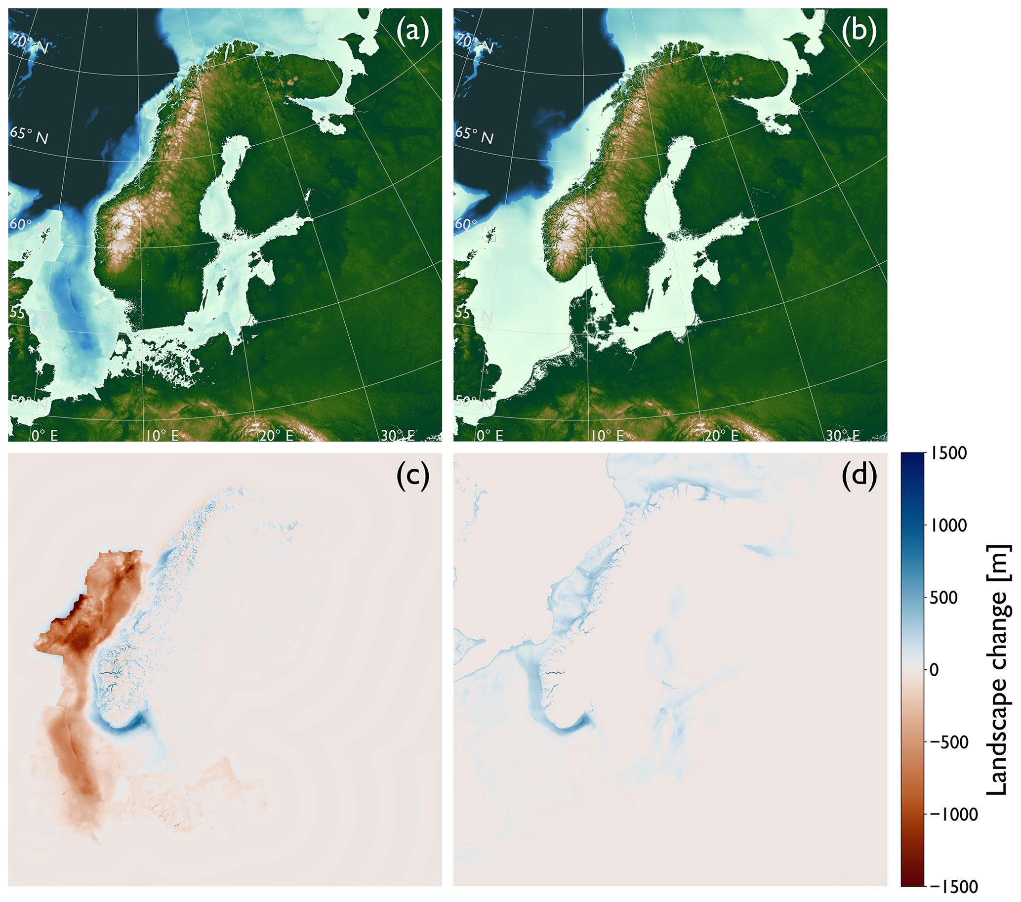
Figure 2Paleo-topographic and bathymetric reconstructions. Panel (a) shows the PREQ experiment and (b) the MLQ experiment. Panels (c) and (d) show the differences between their respective panels above and the modern-day topography and bathymetry.
2.1.2 Topography and bathymetry
The focus of this study is to examine the influence of bed topography on ice-sheet behavior, exemplified by simulating the SIS on landscape configurations representing different periods in the Quaternary. For comparison, we simulate the SIS on modern-day topography and bathymetry over the last glacial cycle in a reference model. The reference experiment uses the global DEM GEBCO 2022 grid (GEBCO Bathymetric Compilation Group, 2022) sampled at 10 km × 10 km for the ice model. (The same grid resolution is used in all experiments.) Because of computational limitations, a model resolution higher than 10 km is not feasible. Having a higher resolution would allow us to resolve glacial morphology in higher detail and could lead to interesting findings regarding the influence of fjord systems in western Norway on ice-sheet dynamics. Here, we focus on larger features, such as the Norwegian Channel, where a 10 km resolution is sufficient. Throughout the model simulations, ice-driven isostasy is handled with a 2D uniform thin elastic plate model (e.g., Pedersen et al., 2014).
The pre-glacial landscape is adopted from Pedersen et al. (2021) and reconstructed using a source-to-sink approach that also considers (i) a component of glacial erosion that has taken place on the inner shelf, (ii) erosion-driven isostasy, and (iii) a component of dynamic topography (Pedersen et al., 2016). For further details on the approach see Pedersen et al. (2021). Here, we extend these previous reconstructions and remove the Quaternary sediment package from all sectors of the North Sea to reconstruct a realistic pre-glacial bathymetry for the entire region (Binzer et al., 1994; Rise et al., 2005; Nielsen et al., 2008; Knox et al., 2010; Gołędowski et al., 2012; Lamb et al., 2018). These additional sediment volumes, from outside of the Norwegian and Danish sectors, are not included in the landscape reconstruction at onshore Scandinavia. The result is a landscape representing a pre-glacial state before any major glaciations in Scandinavia, featuring a large submarine depression in the North Sea and a much narrower continental shelf along the Norwegian margin than at present (Fig. 2a, c). In addition to the PREQ experiment, two sub-experiments are presented: “PREQ-onshore” where only the onshore fjord erosion has been reconstructed (material added to present-day topography) and “PREQ-offshore” where only the offshore deposition has been reconstructed (material removed from present-day bathymetry). Neither of these additional sub-experiments considers the offshore sediment wedge on the shelf. With the sub-experiments we can assess which processes control the behaviors and ice-volume changes observed in the PREQ experiment.
For the middle–late Quaternary experiment, we reconstruct the bathymetry by estimating the volumes of erosion that have been carved into the modern-day seabed by ice streams on the Norwegian shelf and in the Norwegian Channel (Fig. 1). This bathymetric erosion is estimated using the geophysical relief method (e.g., Steer et al., 2012; Pedersen et al., 2021) on the present-day GEBCO 2022 global DEM (GEBCO Bathymetric Compilation Group, 2022), using a grid resolution of 1 km × 1 km and a sliding window radius of 35 km. The resulting filled bathymetry, which also fills fjords to sea level, is adjusted with the flexural isostatic response to loading using gFlex 1.1.1 (Wickert, 2016) with an effective elastic thickness of 15 km. This reconstruction of the Scandinavian morphology is meant to represent a state before the formation of the Norwegian Channel (Fig. 2b, d) and could represent an age of approximately ∼0.5 Ma. This approximate age is supported by the presence of buried mega-scale glacial lineations and drumlins in stratigraphic sequences of the North Sea suggesting that grounded ice has been present since ∼0.5 Ma, whereas the lack of these features in the older strata indicate that early Quaternary glaciations did not ground but only supplied icebergs to the North Sea (Dowdeswell and Ottesen, 2013; Rea et al., 2018).
In this section we start by presenting the results from our reference model simulating the evolution of the SIS on the present-day topography and bathymetry over the last glacial period. Then we present the results of our two experiments with reconstructed topography and bathymetry, as well as how they differ from the reference model. Lastly, we present our findings regarding the formation of the Norwegian Channel.
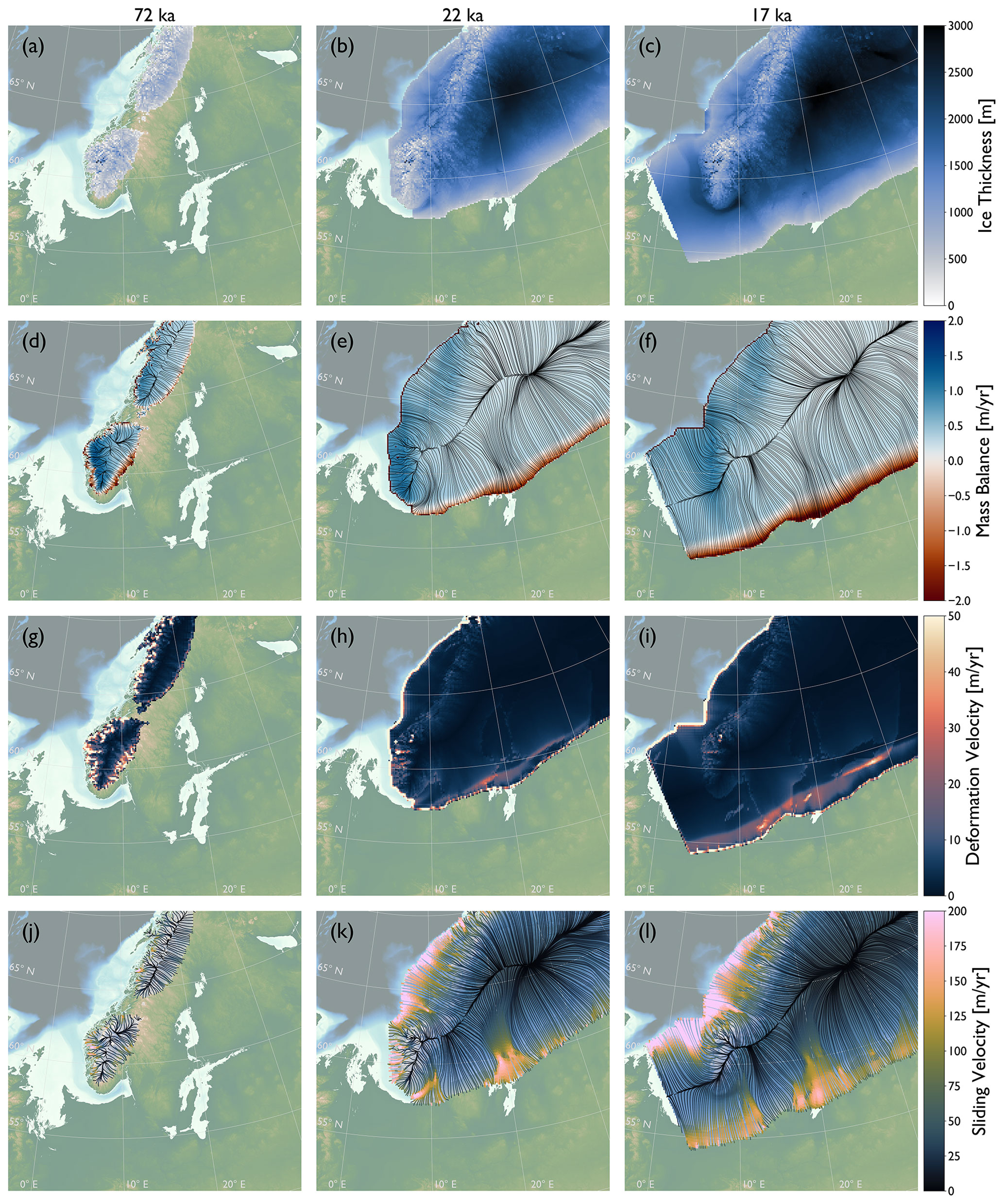
Figure 3Model output from three time slices of the reference experiment. Left column: early glaciation (72 ka); middle column: late–intermediate glaciation (22 ka); right column: glacial maximum (17 ka). Panels (a–c) show ice thickness, (d–f) mass balance, (g–i) depth-averaged deformation velocity, and (j–l) sliding velocity.
3.1 Reference model
To illustrate the spatial and temporal development of the SIS in our model simulations, we present model output from three snapshots in time (Fig. 3): minor ice build-up during early glaciation (72 ka), moderate glacial build-up during intermediate times of the glaciation (22 ka), and the glacial maximum that happens in these simulations at 17 ka. We note that the delayed timing of the glacial maximum in our models compared with the timing of the reconstructed maximum extent in Scandinavia (∼21–19 ka; Hughes et al., 2016) is a direct consequence of the chosen climate forcing, utilizing a glaciation index that peaks at 18 ka. We do not intend here to match the exact timing of the maximum extent (i.e., the LGM). During our simulated early glaciation, ice extent is limited to mountain regions with high topography and high latitude regions in Norway and Sweden (Fig. 3a). Mass balance is positive ∼1.5 m yr−1 in high altitude regions at the Norwegian coast where precipitation is high and temperatures are low (Fig. 3d). Ice deformation and sliding are high (up to >50 and >200 m yr−1, respectively) during early glaciation (Fig. 3g, j) in areas where the thin ice cover is controlled by the underlying topography which includes mountainous regions dissected by fjords and valleys.
During the intermediate glaciation, the ice sheet has advanced onto the shelf region, with grounded ice on the Norwegian margin, and the ice sheet has started to advance into the North Sea through the inner part of the Norwegian Channel (Fig. 3b). The mass balance reaches ∼1 m yr−1 at the west coast of Norway (Fig. 3e), with values <0.5 m yr−1 across most of the ice sheet and negative mass balance at the southwestern margin reaching m yr−1 where the ice is thin and velocities exceed ∼200 m yr−1 (Fig. 3h, k). Along the coastal margin to the west, the mass balance is negative in a narrow zone where floating ice is melting fast. Sliding is notably high, reaching >200 m yr−1 in the inner parts of the Norwegian Channel (Fig. 3k). The ice flow is still steered by topography in the high regions of southern Norway and in the Bothnic Bay, whereas the main divide in northern Scandinavia has shifted east, being largely independent of the underlying topography (Fig. 3e).
During the glacial maximum, the ice sheet reaches a thickness of >3000 m in the central parts (Fig. 3c) with a relatively low positive mass balance along the west coast of Norway (<1 m yr−1; Fig. 3f) with the same general spatial pattern in accumulation and ablation as the intermediate glaciation (Fig. 3e) across the ice sheet. Sliding is high along the northwestern margin of the ice sheet (>200 m yr−1) especially near the shelf break where ice is funneled towards the deeper ocean (Fig. 3l). For a while (∼5000 years) during the maximum expansion, the ice sheet merges with the BIIS in the western part of the North Sea, simulated as an ice wall (Fig. 3f, l). At that time, the ice flow rearranges into a divergent pattern from the ice saddle that emerges between the BIIS and the SIS. Consequently, the ice flows across the Norwegian Channel during the maximum extent instead of being focused in the channel itself, as the ice is diverged southward, driven by the surface slope of the ice sheet under this ice configuration (Fig. 3l). It is worth noting that the reference model captures a realistic placement of the LGM ice divide (Fig. 3f) in accordance with geological observations (Fig. 1; Olsen et al., 2013). Additionally, the ice divide of the saddle across the North Sea during the glacial maximum, when the SIS merges with the BIIS, closely resembles the ice divide suggested by Clark et al. (2022) using a combination of observations and modeling techniques. The glacial maximum ice extent in our reference experiment is within the maximum LGM ice extent (Fig. 1; Hughes et al., 2016), albeit with less ice towards the southern margin and more ice in the northeast.
Figure 4Advance and retreat of the SIS in the reference experiment: (a) ice advance in 5 kyr intervals between model years 72 and 17 ka, and (b) ice retreat in 1 kyr intervals from 17 to 12 ka.
Build-up of the SIS from early mountain glaciation to the glacial maximum happens gradually with grounded ice on the Norwegian shelf forming 10 000 model years before the glacial maximum, and ice advance in the North Sea occurs over just 5000 model years approaching the glacial maximum extent (Fig. 4a). In contrast, the ice retreat is rapid with ice mass loss from the glacial maximum back to a state similar to that of early glaciation happening over just 5000 model years (Fig. 4b).
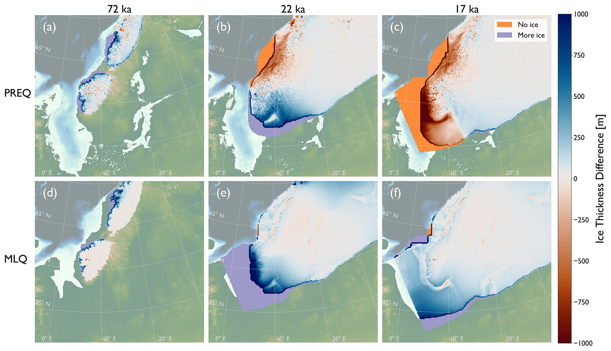
Figure 5Differences in ice thickness for the (a–c) PREQ and (d–f) MLQ experiments compared with the reference experiment. Blue colors mean more ice in this experiment than the reference experiment and red colors mean less ice.
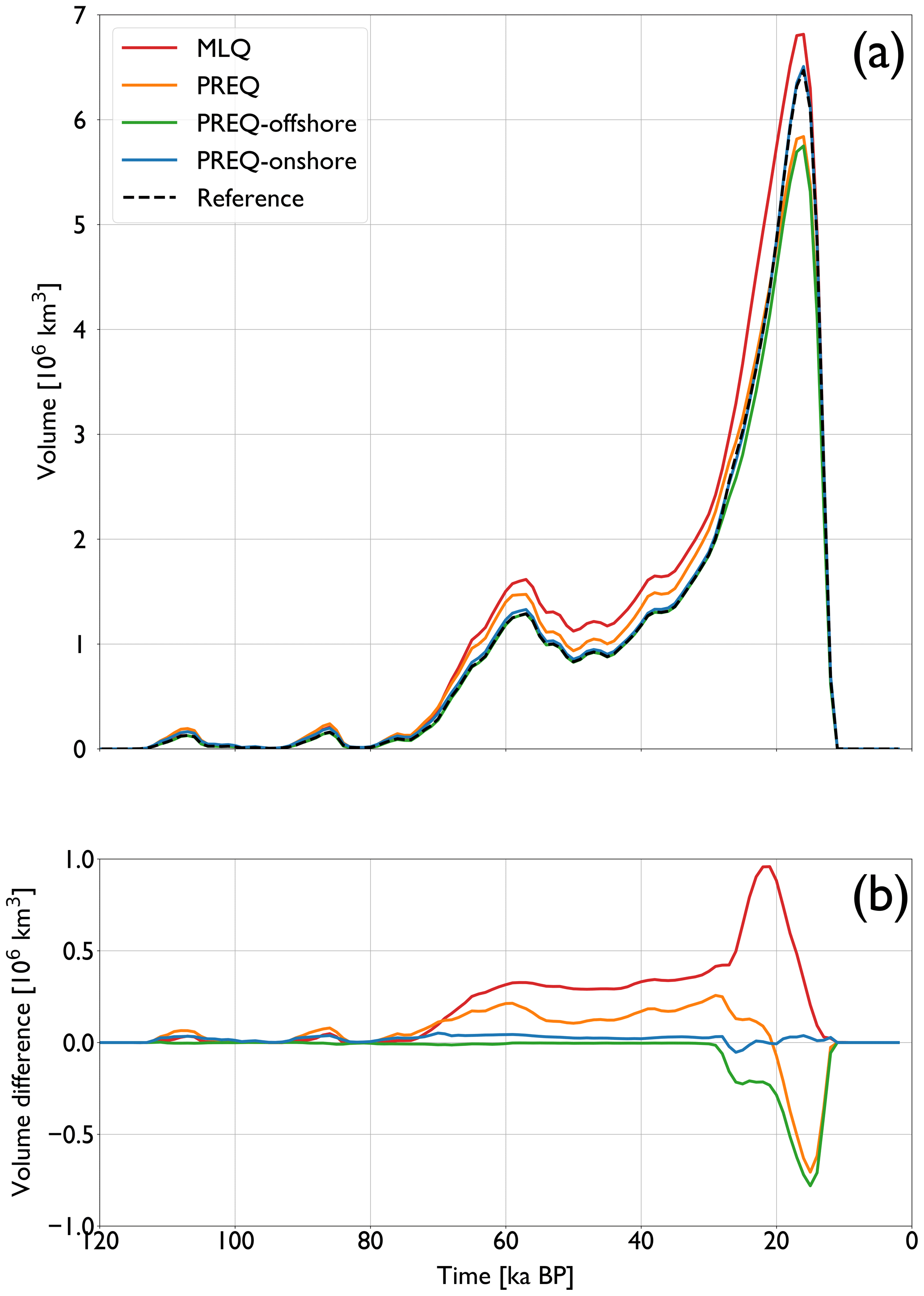
Figure 6Panel (a) shows ice volume over time for the different experiments and (b) shows volume differences between the different experiments and the reference experiment. The dashed black line in (a) is the reference model, the red line is the middle–late Quaternary experiment, and the yellow line is the early Quaternary experiment. The green and blue lines represent the two sub-experiments of the early Quaternary experiment (offshore and onshore landscape changes compared with present day, respectively).
3.2 Results from PREQ and MLQ
In the model simulation representing ice-sheet behavior on an early Quaternary landscape morphology (PREQ; Figs. 2a, 5a, b, c), the ice sheet initially extends further than the reference model (Fig. 5a, purple color), particularly towards the Norwegian coast. At the intermediate stage (Fig. 5b), the ice sheet shows a smaller extent and thickness towards the Norwegian margin (Fig. 5b, orange color), whereas the ice extends further towards the south (Fig. 5b, purple color) with an ice thickness increase of >500 m in some regions. The location of the present-day Norwegian Channel shows a much thinner ice since this bathymetric depression is not present in the PREQ landscape reconstruction (Fig. 5b). At the maximum extent, the ice sheet is smaller both along the western and the southwestern margins (Fig. 5c, orange color), with a general decrease in ice-sheet thickness compared with the reference model (Fig. 5c, red colors). The reduced extent and ice thickness during the maximum extent result in ∼10 % lower maximum ice volume than the reference model (Fig. 6, orange curve). The large difference in ice volume between the PREQ experiment and the reference experiment is largely driven by differences in bathymetry (PREQ-offshore; Fig. 6a, green curve) as changes in topography do not lead to significant differences in ice volume compared with the reference model (PREQ-onshore; Fig. 6a, blue curve).
For the MLQ simulation that represents ice flow on a landscape morphology that existed prior to extensive erosion of the bathymetry by ice streaming (Figs. 2b, 5d, e, f), the ice sheet also starts slightly larger (Fig. 5d, purple color) compared with the reference model. At the intermediate stage, the ice sheet has already extended all the way across the North Sea (Fig. 5e, purple color), showing also a significantly thicker ice sheet in the adjoining regions at onshore Scandinavia. This trend is continued during the maximum extent, where the MLQ ice sheet extends even further, particularly towards the south (Fig. 5f, purple color). In general, the extent of the MLQ ice sheet is not changed along the Norwegian margin, where the width of the shelf has not changed for this simulation (Fig. 5e, f). The increased ice extent and ice thickness in the MLQ simulation result in a maximum ice volume that is ∼25 % more than that of the reference model during the intermediate stage and ∼5 % during the glacial maximum as a direct result of the changed bathymetry (Fig. 6, red curve).
3.3 Sliding in the Norwegian Channel
The erosive power of ice is a product of ice flux over a region with grounded ice (Patton et al., 2022) and is strongly correlated with ice sliding velocity (Cook et al., 2020), which means sliding velocity can be considered a proxy for erosive potential. Here, we explore whether our higher-order ice-sheet model can capture the erosive potential through sliding in the Norwegian Channel in the present-day bathymetry of the reference model and whether the model can predict erosion when the channel is not there in the PREQ and MLQ experiments. The ice dynamics in our reference simulation show significant sliding in the Norwegian Channel in four distinct phases (Fig. 7a, b, c, d). In the early glacial stage, the ice is sliding fast southeast of southern Norway along the deepest part of the channel (Fig. 7a). As the ice approaches maximum extent, the sliding pattern changes because of the different ice flow patterns that arise as an ice saddle emerges in the North Sea when the SIS merges with the BIIS (Fig. 7b). At this stage, ice flows south across the channel from the southern mountains of Norway, following the steepest surface gradient of the ice sheet. Instead, sliding is now mostly concentrated in the outer parts of the Norwegian Channel close to the North Sea Fan (Fig. 7b). During retreat, ice sliding continues in the outer parts of the channel but also becomes prominent along the southern tip of Norway with ice sliding towards the southeast, and in the inner parts of the channel near Oslo Fjord (Fig. 7c). Finally, as the ice sheet retreats further, continued sliding towards the North Sea Fan is complemented by a phase of southward sliding in the channel along the southwestern coast, a region that had not seen significant prior sliding (Fig. 7d). In Fig. 7e–h we show the same time slices for the MLQ experiment. Here, the ice extends further towards the west and has already formed a saddle between the SIS and the BIIS during the initial phase of the glacial cycle (Fig. 7e), and sliding is high towards the shelf break in the region that will later become the outermost part of the Norwegian Channel. Sliding velocities towards the shelf break are consistently high throughout the model simulation (Fig. 7f, h), whereas sliding accelerates in the inner parts of what will become the Norwegian Channel during ice retreat (Fig. 7g). In the last time slice, sliding velocity is lower than in the reference experiment but has the same general pattern (Fig. 7h), with sliding in some regions along the west coast of southern Norway. In Fig. 7i–l we present the time slices for the PREQ experiment. Across all four panels the patterns differ from the reference and MLQ experiments. Instead, we observe high sliding velocities towards the west across where the channel is today (Fig. 7i, j, k). In the last time slice we observe very little sliding as the ice has retreated mostly onshore at this time in the PREQ experiment (Fig. 7l).
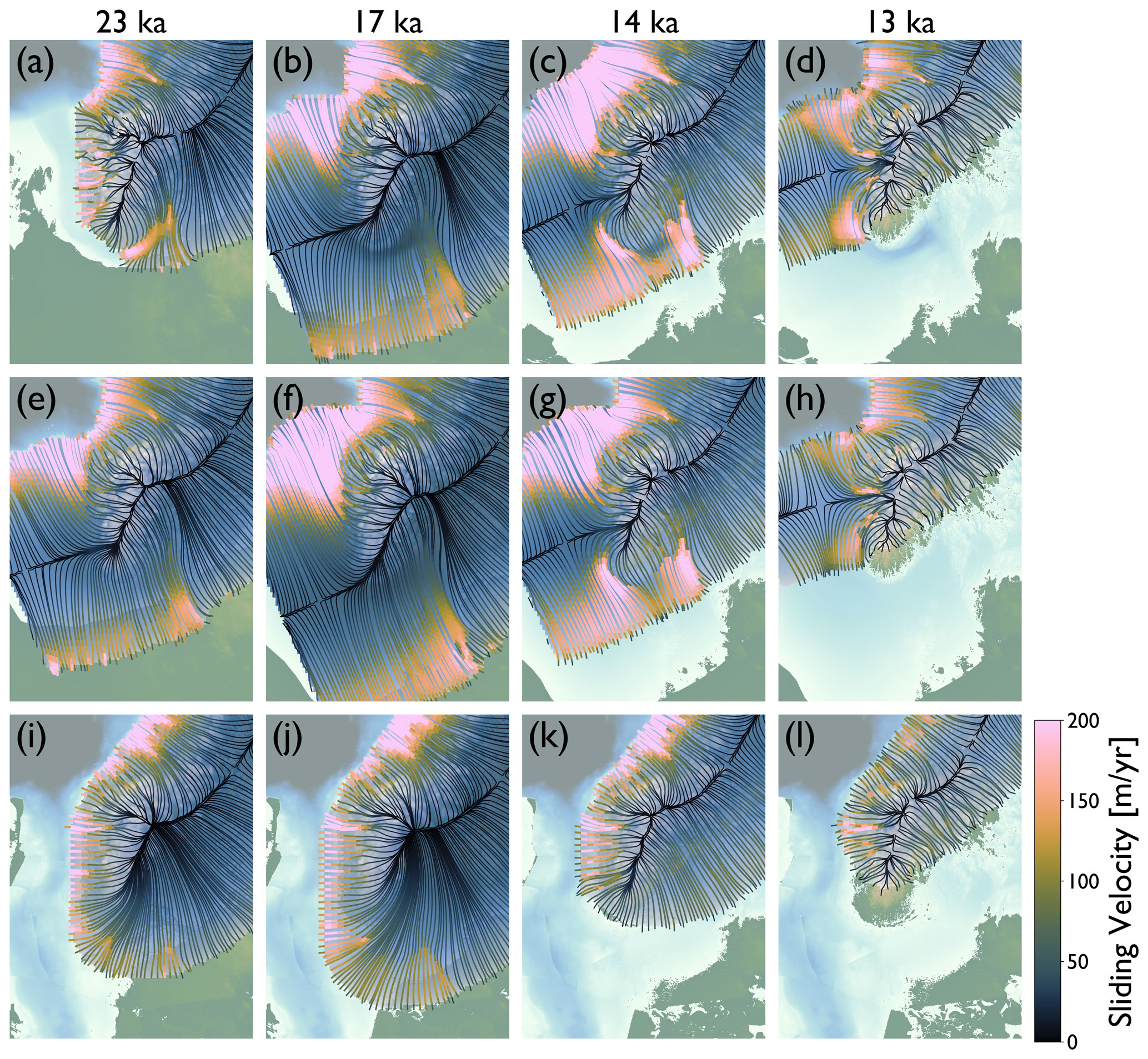
Figure 7Sliding velocity in southwestern Norway for reference model year (a) 23 ka, (b) 17 ka, (c) 14 ka, and (d) 13 ka. Same for the MLQ experiment (e–h) and the PREQ experiment (i–l).
4.1 Ice extent and volume
The ice volume in our reference experiment reaches 6.5 M km3 at the glacial maximum, which is within estimates of SIS and Eurasian ice-sheet volume from previous studies (e.g., Hughes et al., 2016; Patton et al., 2016; Simms et al. 2019). The ice divide of the SIS in the reference experiment is in good agreement with observations (Figs. 1, 3f) which also affirms that our model captures an adequate representation of the ice sheet during the last glacial period. The differences in maximum ice extent between our reference experiment and observations (see Fig. 1; Hughes et al., 2016) can be attributed to the simple mass balance implemented in our model, using linear gradients, that does not capture the complex nature of the regional climate during the last glacial cycle but is an adequate approximation for our purposes. Geological observations suggest that the main ice advance in Denmark approaching the glacial maximum between 20 and 22 ka came from the northeast bringing till deposits of Middle Swedish provenance (Houmark-Nielsen, 2004), whereas the main ice advance into Denmark in our reference experiment comes from the north (Fig. 4a). A possible reason that our model does not capture this dynamic in the southerly ice advance could be the lack of subglacial hydrology in the model which can increase sliding rates (Egholm et al., 2012a). It could also be the lack of a more complex stress-dependent ice viscosity, where the Glen's flow law stress exponent can increase to n≈4 in some areas, which can increase the flow velocity by an order of magnitude (Millstein et al., 2022). These effects could be important especially in the southern parts of the ice sheet where the ice is thin and fast flowing during advance (Fig. 3c, i). Here, an even faster and thinner ice might be more sensitive to the low-relief topography of southern Scandinavia leading to a more westerly ice flow from Sweden into Denmark in agreement with the observations.
We cannot directly compare the ice extents in our experiments with reconstructions of past SIS extent as we use the same climate forcing between experiments, but we can assess whether differences in past ice-sheet extents follow the same trends as we see in this study that are based solely on differences in morphology. Batchelor et al. (2019) use empirical data to evaluate past Northern Hemisphere glacial extents and suggest best-estimate maximum southern extents of the MIS 12 (429–477 ka), MIS 16 (622–677 ka), and MIS 20–24 (790–928 ka) ice sheets to be somewhere between the best-estimate maximum MIS 6 extent and the LGM extent (132–190 ka; Fig. 1, dashed red line and black line), although the MIS 16 and MIS 20–24 maximum ice-sheet extents are highly uncertain. These reconstructions are based on very limited observations and, in some cases (e.g., MIS 12 and MIS 16), the estimates are mostly based on similarities in the δ18O curve (Batchelor et al., 2019). We show with this study that purely morphological differences in bathymetry between the last glacial period and ∼0.5 Ma (MLQ experiment, similar in time to MIS 12 and MIS 16) allow for larger ice-sheet extents simply owing to geomorphic changes during this time period. This suggests that both climatic and topographic forcings might have caused these (possibly) large ice extents of the middle–late Quaternary (MIS 12, MIS 16, and MIS 20–24). Indeed, our results showcase that a smooth bathymetry in the North Sea region (i.e., lacking glacial morphology), such as before the inception of the Norwegian Channel, could lead to earlier and more extensive southerly ice advance within a glacial period (Fig. 5e). On the other hand, our simulation of early Quaternary glaciations suggests that ice build-up across the North Sea was not plausible at this early stage of glacial landscape evolution. Indeed, in the PREQ experiment we found that the SIS could extend no further than the continental shelf during the early Quaternary (Fig. 5b, c). This is consistent with a study of buried glacial landforms in the central North Sea documenting iceberg plough marks in early Quaternary sediments (Dowdeswell et al., 2013; Rea et al., 2018). Our reconstructed early Quaternary ice sheet would have supplied icebergs that created these plough marks.
The differences we find in ice volume at the maximum glacial extent (∼5 % higher for MLQ, ∼10 % lower for PREQ) illustrate how differences in morphology affect ice volume independently of climate forcing. This has implications for the proxies we use for ice-volume history. Clearly the effect of glacial morphology explored here is local in nature, whereas the LR04 Benthic Stack we use as a glacial index and a proxy for ice volume is a global proxy. In addition, local ice volume also depends on global atmospheric circulation patterns which can lead to asynchronous development of the ice sheets during a glacial period (e.g., Liakka et al., 2016) that will also influence ice-sheet volume between glacial cycles. But landscape evolution has also played a significant role along other ice-sheet margins through the Quaternary, for example, leading to increased ice-sheet advance across marine sectors of the Antarctic ice sheet (Hochmuth and Gohl, 2019; Hochmuth et al., 2020). It should also be noted that the lack of ice shelves in our model could have a significant impact on grounded ice volume as buttressing effects of ice shelves can stabilize and advance grounding lines across the marine sectors of an ice sheet (e.g., Gasson et al., 2018). Nevertheless, according to this study, landscape morphology alone can account for up to ∼10 % difference in ice volume between glacial cycles for the Scandinavian region (∼25 % during ice build-up), implying that glacial landscape evolution could be an overlooked mechanism impacting local and global ice volume and thereby the interpretation of δ18O curves. This emphasizes the added uncertainty of landscape morphology on Quaternary ice-sheet reconstructions.
4.2 Formation of the Norwegian Channel
It is uncertain how and when the Norwegian Channel was formed, with studies estimating the time of formation to be between ∼0.35 and 1.1 Ma – with more recent studies suggesting younger ages (e.g., Sejrup et al., 2003; Hjelstuen et al., 2012; Løseth et al., 2022). In this study, we have assumed that the entirety of the Norwegian Channel formed after ∼0.5 Ma (MLQ). For the last glacial cycle, it has previously been proposed that the Norwegian Channel Ice Stream (NCIS) was active in stages but mainly during the LGM (e.g., Sejrup et al., 1998, 2003). According to an earlier study (Sejrup et al., 2016), ice streaming in the outer parts of the channel near the shelf break started close to the LGM with increased activity promoting ice retreat around 19 ka because of increased ice mass loss. The retreat translated southwards over time as the SIS unzipped from the adjacent BIIS after which ice streaming was mostly confined to the main trunk of the channel (Sejrup et al., 2016). A previous modeling study also suggests that the NCIS was active in stages with streaming in the inner parts of the channel leading up to, and became inactive during, the glacial maximum because of the saddle forming from the merging of the BIIS and the SIS (Boulton and Hagdorn, 2006). We find in our reference model with present-day bathymetry that ice streaming was active in the inner parts of the channel before the saddle formed between the BIIS and the SIS, after which ice streaming velocity increased dramatically in the outer parts of the Norwegian Channel near the shelf break and decreased in the inner parts of the Norwegian Channel as the saddle formed, consistent with other studies based on observations of, for example, subglacial landforms combined with dated sediment cores (Sejrup et al., 2016). On the other hand, our reference experiment does not mimic at any time an NCIS spanning the entire trunk of the Norwegian Channel, which would significantly contribute to ice mass loss from rapid grounding line retreat as is supported by observations (Sejrup et al., 2016). However, with this model setup we cannot rule out the occurrence of continuous ice streaming in the entire Norwegian Channel after the LGM. Indeed, some processes central to reproducing realistic ice stream behavior are not included in iSOSIA, such as enhanced basal melt owing to basal friction, leading to accelerated thinning in regions with rapid ice sliding as well as effects of internal friction and temperature advection on ice viscosity which can greatly amplify sliding velocities (Millstein et al., 2022; Bondzio et al., 2017). These mechanisms could contribute to highly elevated sliding velocities, especially in the NCIS, and could facilitate a propagation of the streaming activity we observe in the outer parts of the channel to the inner parts. In addition, the static ice wall we use to simulate the merging SIS and BIIS introduces a highly persistent ice saddle, which may introduce unrealistic streaming patterns and ice extent during NCIS retreat (Fig. 7c, d, g, h). Indeed, a previous study facilitates the retreat of the Norwegian Channel, with a negative surface mass balance anomaly in the southern sector of the North Sea, in order to match the ice margin to empirical reconstructions (Gandy et al., 2021).
Despite the Norwegian Channel being filled with sediment in the reconstructed bathymetry of our MLQ experiment, we find an ice streaming pattern that is comparable to that of the reference model for several parts of the model (Fig. 7a, b, c, d, e, f, g, h). Specifically, in the MLQ experiment, high sliding velocities are also present in what will become the inner part of the Norwegian Channel as the ice begins to advance offshore (Video 3 in the Video Supplement), although the ice velocity will be less focused compared with the reference model where the depression of the Norwegian Channel steers the ice even further (Fig. 7a). We stress, however, that because the ice advances faster offshore in the MLQ experiment, this sliding in the inner parts of what will become the Norwegian Channel happens prior to 23 ka (Fig. 7e; Video 3 in the Video Supplement). The MLQ experiment also shows high sliding rates where the outer part of the Norwegian Channel will form towards the shelf break (Fig. 7e, f, g, h), even extending further back in time than the reference experiment (Fig. 7a, e). This steering of ice towards the north–northwest in the MLQ experiment, steering which takes place before a bathymetric depression is formed, is mainly controlled by the steeper ice-surface gradient that occurs towards the shelf break in this simulation, when the ice advances into the offshore region and approaches the shelf break much earlier than in the reference experiment. This ice flow pattern begins before the saddle between the BIIS and the SIS formed but is amplified further by the ice saddle that forms in the North Sea as the ice cannot advance further towards the west (Video 3 in the Video Supplement). Our models can thus explain the initial formation of the Norwegian Channel in the innermost and outermost parts, starting from a bathymetry that had no prior imprint of the present-day channel. The MLQ experiment also shows sliding in other parts of what will become the Norwegian Channel later in the model simulation (e.g., Fig. 7g, h). However, we find these results less robust owing to the limitations of our model setup during the deglaciation.
On the other hand, the PREQ experiment showed no ice flow or sliding patterns similar to those of the reference model in the region that would later become the Norwegian Channel. Indeed, ice flow and sliding are at all times perpendicular to the future Norwegian Channel because of the sediment wedge that existed along the Norwegian coast and a steep ice-surface gradient towards the North Sea, sustained by the deep bathymetry of the North Sea that prevented grounded ice. Therefore, we find it likely that the carving of the Norwegian Channel could not have been initiated before the North Sea basin had been sufficiently filled with sediments. Instead, we find it plausible that the Norwegian Channel formed during multiple glacial periods since ∼0.5 Ma, consistent with a recent study indicating that the channel was formed prior to ∼0.35 Ma (Løseth et al., 2022). Our results are also in agreement with studies on the North Sea Fan (NCIS depocenter), suggesting that 90 % of the sediments in this fan are younger than ∼0.5 Ma (Hjelstuen et al., 2012).
We used a higher-order ice-sheet model to investigate the effects of landscape morphology on the SIS evolution and dynamics. Three different experiments where conducted: (i) a reference experiment resembling the last glacial cycle using modern-day topography and bathymetry, (ii) a middle–late Quaternary experiment with glacial morphological features in the present-day bathymetry filled with sediment, and (iii) a pre-Quaternary experiment simulating the SIS on a reconstructed pre-glacial topography and bathymetry. We found in the MLQ experiment that removing glacial morphological features in the bathymetry allowed for faster and further southward expansion at similar climatic conditions allowing for a larger ice sheet. Contrary to this, we found in the PREQ experiment that the early Quaternary bathymetry did not allow for the SIS to advance as far westward and southward, thereby limiting the size of early glaciations and preventing a merging of the BIIS and the SIS. Looking at the prominent glacio-morphological feature, the Norwegian Channel, we found that the PREQ experiment did not allow for significant ice streaming in this area and that the channel was more likely formed after the North Sea was filled in with glacial sediments. Furthermore, our results suggest that ice streaming occurred in distinct stages along the trunk of the channel with high ice sliding in the inner parts before the LGM and sliding in the outer parts of the channel close to the shelf break during the LGM. Our results also show that sliding in the inner parts of the channel ceased because of divergent ice flow when the BIIS and the SIS merged and formed a saddle across the North Sea.
Code and/or data will be made available upon request.
Sliding speed and flow lines (Fig. 7) for model years 35 to 12 ka for all three experiments are available at https://doi.org/10.7910/DVN/KLCMEG (Jungdal-Olesen, 2024).
GJO: conceptualization, methodology, software, formal analysis, writing – original draft, and visualization. VKP: conceptualization, methodology, supervision, writing – review and editing, and funding acquisition. JLA: writing – review and editing, and visualization. AB: resources and writing – review and editing.
The contact author has declared that none of the authors has any competing interests.
Publisher's note: Copernicus Publications remains neutral with regard to jurisdictional claims made in the text, published maps, institutional affiliations, or any other geographical representation in this paper. While Copernicus Publications makes every effort to include appropriate place names, the final responsibility lies with the authors.
This article is part of the special issue “Icy landscapes of the past”. It is not associated with a conference.
The authors thank Leif Rise, Bartosz Gołędowski, Tove Nielsen, and Mads Huuse for sediment thickness data. We thank Anne Munck Solgaard for the useful comments on the manuscript.
This research has been supported by the Villum Fonden (grant no. 15467).
This paper was edited by Atle Nesje and reviewed by David Sugden, Rosie Archer, and Henry Patton.
Anderson, R. S., Dühnforth, M., Colgan, W., and Anderson, L.: Far-flung moraines: Exploring the feedback of glacial erosion on the evolution of glacier length, Geomorphology, 179, 269–285, https://doi.org/10.1016/j.geomorph.2012.08.018, 2012.
Bart, P. J., Mullally, D., and Golledge, N. R.: The influence of continental shelf bathymetry on Antarctic ice sheet response to climate forcing, Global Planet. Change, 142, 87–95, https://doi.org/10.1016/j.gloplacha.2016.04.009, 2016.
Batchelor, C. L., Margold, M., Krapp, M., Murton, D. K., Dalton, A. S., Gibbard, P. L., Stokes, C. R., Murton, J. B., and Manica, A.: The configuration of northern hemisphere ice sheets through the Quaternary, Nat. Commun., 10, 3713, https://doi.org/10.1038/s41467-019-11601-2, 2019.
Binzer, K., Stockmarr, J., and Lykke-Andersen, H.: Pre-quaternary Surface Topography of Denmark, Geological survey of Denmark, map series no. 44, 1994.
Bondzio, J. H., Morlighem, M., Seroussi, H., Kleiner, T., Rückamp, M., Mouginot, J., Moon, T., Larour, E. Y., and Humbert, A.: The mechanisms behind jakobshavn isbræ's acceleration and mass loss: A 3-d thermomechanical model study, Geophys. Res. Lett., 44, 6252–6260, https://doi.org/10.1002/2017GL073309, 2017.
Boulton, G. and Hagdorn, M.: Glaciology of the british isles ice sheet during the last glacial cycle: form, flow, streams and lobes, Quaternary Sci. Rev., 25, 3359–3390, https://doi.org/10.1016/j.quascirev.2006.10.013, 2006.
Clague, J. J., Barendregt, R. W., Menounos, B., Roberts, N. J., Rabassa, J., Martinez, O., Ercolano, B., Corbella, H., and Hemming, S. R.: Pliocene and early Pleistocene glaciation and landscape evolution on the Patagonian steppe, santa cruz province, Argentina, Quaternary Sci. Rev., 227, 105992, https://doi.org/10.1016/j.quascirev.2019.105992, 2020.
Clark, C. D., Ely, J. C., Hindmarsh, R. C. A., Bradley, S., Ignéczi, A., Fabel, D., Ó Cofaigh, C., Chiverrell, R. C., Scourse, J., Benetti, S., Bradwell, T., Evans, D. J. A., Roberts, D. H., Burke, M., Callard, S. L., Medialdea, A., Saher, M., Small, D., Smedley, R. K., and Wilson, P.: Growth and retreat of the last British–Irish Ice Sheet, 31 000 to 15 000 years ago: the BRITICE-CHRONO reconstruction, Boreas, 51, 699–758, https://doi.org/10.1111/bor.12594, 2022.
Cook, S. J., Swift, D. A., Kirkbride, M. P., Knight, P. G., and Waller, R. I.: The empirical basis for modelling glacial erosion rates, Nat. Commun., 11, 759, https://doi.org/10.1038/s41467-020-14583-8, 2020.
Dee, D. and National Center for Atmospheric Research Staff (Eds.): The Climate Data Guide: ERA-Interim, https://climatedataguide.ucar.edu/climate-data/era-interim (last access: 27 August 2023), last modified: 7 November 2022.
Dowdeswell, J. A. and Ottesen, D.: Buried iceberg ploughmarks in the early quaternary sediments of the central north sea: A two-million year record of glacial influence from 3d seismic data, Mar. Geol., 344, 1–9, https://doi.org/10.1016/j.margeo.2013.06.019, 2013.
Egholm, D. L., Nielsen, S. B., Pedersen, V. K., and Lesemann, J. E.: Glacial effects limiting mountain height, Nature, 460, 884–887, https://doi.org/10.1038/nature08263, 2009.
Egholm, D. L., Knudsen, M. F., Clark, C. D., and Lesemann, J. E.: Modeling the flow of glaciers in steep terrains: The integrated second-order shallow ice approximation (iSOSIA), J. Geophys. Res.-Earth, 116, 1–16, https://doi.org/10.1029/2010JF001900, 2011.
Egholm, D. L., Pedersen, V. K., Knudsen, M. F., and Larsen, N. K.: Coupling the flow of ice, water, and sediment in a glacial landscape evolution model, Geomorphology, 141–142, 47–66, https://doi.org/10.1016/j.geomorph.2011.12.019, 2012a.
Egholm, D. L., Pedersen, V. K., Knudsen, M. F., and Larsen, N. K.: On the importance of higher order ice dynamics for glacial landscape evolution, Geomorphology, 141–142, 67–80, https://doi.org/10.1016/j.geomorph.2011.12.020, 2012b.
Egholm, D. L. and Nielsen, S. B.: An adaptive finite volume solver for ice sheets and glaciers, J. Geophys. Res., 115, F01006, https://doi.org/10.1029/2009JF001394, 2010.
Egholm, D. L., Jansen, J. D., Brædstrup, C. F., Pedersen, V. K., Andersen, J. L., Ugelvig, S. V., Larsen, N. K., and Knudsen, M. F.: Formation of plateau landscapes on glaciated continental margins, Nat. Geosci. 10, 592–597, https://doi.org/10.1038/NGEO2980, 2017.
Gandy, N., Gregoire, L. J., Ely, J. C., Cornford, S. L., Clark, C. D., and Hodgson, D. M.: Collapse of the Last Eurasian Ice Sheet in the North Sea Modulated by Combined Processes of Ice Flow, Surface Melt, and Marine Ice Sheet Instabilities, J. Geophys. Res.-Earth., 126, e2020JF005755, https://doi.org/10.1029/2020JF005755, 2021.
Gasson, E. G. W., Deconto, R. M., Pollard, D., and Clark, C. D: Numerical simulations of a kilometre-thick Arctic ice shelf consistent with ice grounding observations, Nat. Commun., 9, 1510, https://doi.org/10.1038/s41467-018-03707-w, 2018.
GEBCO Bathymetric Compilation Group: The GEBCO_2022 Grid – a continuous terrain model of the global oceans and land, NERC EDS British Oceanographic Data Centre NOC [data set], https://doi.org/10.5285/e0f0bb80-ab44-2739-e053-6c86abc0289c, 2022.
Gladstone, R., Moore, J., Wolovick, M., and Zwinger, T.: Sliding conditions beneath the Antarctic Ice Sheet, EGU General Assembly 2020, Online, 4–8 May 2020, EGU2020-7038, https://doi.org/10.5194/egusphere-egu2020-7038, 2020.
Gołędowski, B., Nielsen, S. B., and Clausen, O. R.: Patterns of Cenozoic sediment flux from western Scandinavia, Basin Res., 24, 377–400, https://doi.org/10.1111/j.1365-2117.2011.00530.x, 2012.
Hall, A. M., Ebert, K., Kleman, J., Nesje, A., and Ottesen, D.: Selective glacial erosion on the Norwegian passive margin, Geology, 41, 1203–1206, https://doi.org/10.1130/G34806.1, 2013.
Han, H. K., Gomez, N., Pollard, D., and DeConto, R.: Modeling northern hemispheric ice sheet dynamics, sea level change, and solid earth deformation through the last glacial cycle, J. Geophys. Res.-Earth. 126, 1–15, https://doi.org/10.1029/2020JF006040, 2021.
Hjelstuen, B. O., Nygard, A., Sejrup, H. P., and Haflidason, H.: Quaternary denudation of southern fennoscan- dia – evidence from the marine realm, Boreas, 41, 379–390, https://doi.org/10.1111/j.1502-3885.2011.00239.x, 2012.
Hochmuth, K. and Gohl, K.: Seaward growth of Antarctic continental shelves since establishment of a continent-wide ice sheet: Patterns and mechanisms, Palaeogeogr. Palaeocl., 520, 44–54, https://doi.org/10.1016/j.palaeo.2019.01.025, 2019.
Hochmuth, K., Gohl, K., Leitchenkov, G., Sauermilch, I., Whittaker, J. M., Uenzelmann-Neben, G., Davy, B., and de Santis, L.: The Evolving Paleobathymetry of the Circum-Antarctic Southern Ocean Since 34 Ma: A Key to Understanding Past Cryosphere-Ocean Developments, Geochem. Geophy. Geosy., 21, e2020GC009122, https://doi.org/10.1029/2020GC009122, 2020.
Houmark-Nielsen, M.: The Pleistocene of Denmark: a review of stratigraphy and glaciation history, Dev. Quat. Sci., 2, 35–46, https://doi.org/10.1016/S1571-0866(04)80055-1, 2004.
Hughes, A. L., Gyllencreutz, R., Öystein S. Lohne, Mangerud, J., and Svendsen, J. I.: The last eurasian ice sheets – a chronological database and time-slice reconstruction, dated-1, Boreas, 45, 1–45, https://doi.org//10.1111/bor.12142, 2016.
Hughes, P. D. and Gibbard, P. L.: Global glacier dynamics during 100 ka pleistocene glacial cycles, Quaternary Res., 90, 222–243, https://doi.org/10.1017/qua.2018.37, 2018.
Hughes, T., Denton, G. H., and Grosswald, M.: Was there a late-würm arctic ice sheet?, Nature, 266, 596–602, https://doi.org/10.1038/266596a0, 1977.
Jakobsson, M., Nilsson, J., Anderson, L., Backman, J., Björk, G., Cronin, T. M., Kirchner, N., Koshurnikov, A., Mayer, L., Noormets, R., O'Regan, M., Stranne, C., Ananiev, R., Macho, N. B., Cherniykh, D., Coxall, H., Eriksson, B., Floden, T., Gemery, L., Gustafsson, O., Jerraegan, M., Stranne, C., Ananiev, R., Macho, N. B., Cherniykh, D., Coxall, H., Eriksson, B., Floden, T., Gemery, L., Jerram, K., Johansson, C., Khortov, A., Mohammad, R., and Semiletov, I.: Evidence for an ice shelf covering the central arctic ocean during the penultimate glaciation, Nat. Commun., 7, 10365, https://doi.org/10.1038/ncomms10365, 2016.
Jungclaus, J., Mikolajewicz, U., Kapsch, M. L., DíAgostino, R., Wieners, K. H., Giorgetta, M., Reick, C., Esch, M., Bittner, M., Legutke, S., Schupfner, M., Wachsmann, F., Gayler, V., Haak, H., de Vrese, P., Raddatz, T., Mauritsen, T., von Storch, J. S., Behrens, J., Brovkin, V., Claussen, M., Crueger, T., Fast, I., Fiedler,S., Hagemann, S., Hohenegger, C., Jahns, T., Kloster, S., Kinne, S., Lasslop, G., Kornblueh, L., Marotzke,J., Matei, D., Meraner, K., Modali, K., Mgemann, S., Hohenegger, C., Jahns, T., Kloster, S., Kinne, S., Lasslop, G., Kornblueh, L., Marotzke, J., Matei, D., Meraner, K., Modali, K., Müller, W., Nabel, J., Notz, D., Peters-von Gehlen, K., Pincus, R., Pohlmann, H., Pongratz, J., Rast, S., Schmidt, W., Nabel, J., Notz, D., Peters-von Gehlen, K., Pincus, R., Pohlmann, H., Pongratz, J., Rast, S., Schmidt, H., Schnur, R., Schulzweida, U., Six, K., Stevens, B., Voigt, A., and Roeckner, E.: Mpi-m mpi-esm1.2-lr model output prepared for cmip6 pmip lgm, Earth System Grid Federation [data set], https://doi.org/10.22033/ESGF/CMIP6.6642, 2019.
Jungdal-Olesen, G.: Supplementary videos, V1, Harvard Dataverse [video], https://doi.org/10.7910/DVN/KLCMEG, 2024.
Kaplan, M. R., Hein, A. S., Hubbard, A., and Lax, S. M.: Can glacial erosion limit the extent of glaciation?, Geomorphology, 103, 172–179, 2009.
Kessler, M. A., Anderson, R. S., and Briner, J. P.: Fjord insertion into continental margins driven by topographic steering of ice, Nat. Geosci., 1, 365–369, https://doi.org/10.1038/ngeo201, 2008.
Knox, R. W. O. B., Bosch, J. H. A., Rasmussen, E. S., Heilmann-Clausen, C., Hiss, M., De Lugt, I. R., Kasińksi, J., King, C., Köthe, A., Słodkowska, B., Standke, G., and Vandenberghe, N.: Cenozoic, in: Petroleum Geological Atlas of the Southern Permian Basin Area, edited by: Doornenbal, J. C. and Stevenson, A. G., EAGE Publications, The Netherlands, 211–223, 2010.
Lamb, R. M., Harding, R., Huuse, M., Stewart, M., and Brocklehurst, S. H.: The early quaternary north sea basin, J. Geol. Soc. London, 175, 275–290, https://doi.org/10.1144/jgs2017-057, 2018.
Liakka, J., Löfverström, M., and Colleoni, F.: The impact of the North American glacial topography on the evolution of the Eurasian ice sheet over the last glacial cycle, Clim. Past, 12, 1225–1241, https://doi.org/10.5194/cp-12-1225-2016, 2016.
Lindstrom, D. R. and MacAyeal, D. R.: Paleoclimatic constraints on the maintenance of possible ice-shelf cover in the Norwegian and Greenland seas, Paleoceanography, 1, 313–337, https://doi.org/10.1029/PA001i003p00313, 1986.
Lisiecki, L. E. and Raymo, M. E.: A pliocene-pleistocene stack of 57 globally distributed benthic 18o records, Paleoceanography, 20, 1–17, https://doi.org/10.1029/2004PA001071, 2005.
Løseth, H., Nygard, A., Batchelor, C. L., and Fayzullaev, T.: A regionally consistent 3d seismic-stratigraphic framework and age model for the quaternary sediments of the northern north sea, Mar. Petrol. Geol., 142, 105766, https://doi.org/10.1016/j.marpetgeo.2022.105766, 2022.
MacGregor, K. R., Anderson, R. S., and Waddington, E. D.: Numerical modeling of glacial erosion and headwall processes in alpine valleys, Geomorphology, 103, 189–204, https://doi.org/10.1016/j.geomorph.2008.04.022, 2009.
Magrani, F., Valla, P. G., and Egholm, D.: Modelling alpine glacier geometry and subglacial erosion patterns in response to contrasting climatic forcing, Earth Surf. Processes, 47, 1054–1072, https://doi.org/10.1002/esp.5302, 2022.
Mas e Braga, M., Jones, R. S., and Bernales, J.: A thicker Antarctic ice stream during the mid-Pliocene warm period, Commun. Earth Environ., 4, 321, https://doi.org/10.1038/s43247-023-00983-3, 2023.
Millan, R., Mouginot, J., Rabatel, A., and Morlighem, M.: Ice velocity and thickness of the world's glaciers, Nat. Geosci., 15, 124–129, https://doi.org/10.1038/s41561-021-00885-z, 2022.
Millstein, J. D., Minchew, B. M., and Pegler, S. S.: Ice viscosity is more sensitive to stress than commonly Assumed, Commun. Earth Environ., 3, 57, https://doi.org/10.1038/s43247-022-00385-x, 2022.
Nielsen, T., Mathiesen, A., and Bryde-Auken, M.: Base quaternary in the danish parts of the north sea and Skagerrak, Geol. Surv. Den. Greenl., 37–40, https://doi.org/10.34194/geusb.v15.5038, 2008.
Olsen, L., Sveian, H., Ottesen, D., and Rise, L.: Quaternary glacial, interglacial and interstadial deposits of norway and adjacent onshore and offshore areas, Geol. Surv. Nor. Spec. Pub, 13, 79–144, https://www.ngu.no/upload/Publikasjoner/Special publication/SP13_s79-144.pdf (last access: 4 April 2024), 2013.
Patton, H., Hubbard, A., Andreassen, K., Winsborrow, M., and Stroeven, A. P.: The build-up, configuration, and dynamical sensitivity of the eurasian ice-sheet complex to late weichselian climatic and oceanic forcing, Quaternary Sci. Rev., 153, 97–121, https://doi.org/10.1016/j.quascirev.2016.10.009, 2016.
Patton, H., Hubbard, A., Heyman, J., Alexandropoulou, N., Lasabuda, A., and Stroeven, A.P.: The extreme yet transient nature of glacial erosion, Nat. Commun., 13, 7377, https://doi.org/10.1038/s41467-022-35072-0, 2022.
Paxman, G. J. G., Jamieson, S. S. R., Hochmuth, K., Gohl, K., Bentley, M. J., Leitchenkov, G., and Ferraccioli, F.: Reconstructions of Antarctic topography since the Eocene–Oligocene boundary, Palaeogeogr. Palaeocl., 535, 109346, https://doi.org/10.1016/j.palaeo.2019.109346, 2019.
Pedersen, V. and Egholm, D.: Glaciations in response to climate variations preconditioned by evolving topography, Nature, 493, 206–210, https://doi.org/10.1038/nature11786, 2013.
Pedersen, V. K., Huismans, R. S., Herman, F., and Egholm, D. L.: Controls of initial topography on temporal and spatial patterns of glacial erosion, Geomorphology, 223, 96–116, https://doi.org/10.1016/j.geomorph.2014.06.028, 2014.
Pedersen, V. K., Huismans, R. S., and Moucha, R.: Isostatic and dynamic support of high topography on a north atlantic passive margin, Earth Planet. Sc. Lett., 446, 1–9, https://doi.org/10.1016/j.epsl.2016.04.019, 2016.
Pedersen, V. K., Knutsen, Å. K., Pallisgaard-Olesen, G., Andersen, J. L., Moucha, R., and Huismans, R. S.: Widespread glacial erosion on the scandinavian passive margin, Geology, 49, 1004–1008, https://doi.org/10.1130/G48836.1, 2021.
Pendergrass, A., Wang, J., and National Center for Atmospheric Research Staff (Eds.): The Climate Data Guide: GPCP (Monthly): Global Precipitation Climatology Project, https://climatedataguide.ucar.edu/climate-data/gpcp-monthly-global-precipitation-climatology-project (last access: 3 September 2023), last modified 7 November 2022.
Rea, B. R., Newton, A. M. W., Lamb, R. M., Harding, R., Bigg, G. R., Rose, P., Spagnolo, M., Huuse, M., Cater, J. M. L., Archer, S., Buckley, F., Halliyeva, M., Huuse, J., Cornwell, D. G., Brocklehurst, S. H., and Howell, J. A.: Extensive marine-terminating ice sheets in europe from 2.5 million years ago, Sci. Adv., 4, 6, https://doi.org/10.1126/sciadv.aar8327, 2018.
Rise, L., Ottesen, D., Berg, K., and Lundin, E.: Large-scale development of the mid-norwegian margin during the last 3 million years, Mar. Petr. Geol., 22, 33–44, https://doi.org/10.1016/j.marpetgeo.2004.10.010, 2005.
Sejrup, H. P., Landvik, J. Y., Larsen, E., Janockom, J., Eiriksson, J., and King, E.: The jæren area, a border zone of the norwegian channel ice stream, Quaternary Sci. Rev., 17, 801–812, https://doi.org/10.1016/S0277-3791(98)00019-5, 1998.
Sejrup, H. P., Larsen, E., Haflidason, H., Berstad, I. M., Hjelstuen, B. O., Jonsdottir, H. E., King, E. L., Landvik, J., Longva, O., Nygard, A., Ottesen, D., Raunholm, S., Rise, L., and Stalsberg, K.: Configuration, history and impact of the norwegian channel ice stream, Boreas, 32, 18–36, https://doi.org/10.1080/03009480310001029, 2003.
Sejrup, H. P., Clark, C. D., and Hjelstuen, B. O.: Rapid ice sheet retreat triggered by ice stream debuttressing: Evidence from the north sea, Geology, 44, 355–358, https://doi.org/10.1130/G37652.1, 2016.
Simms, A. R., Lisiecki, L., Gebbie, G., Whitehouse, P. L., and Clark, J. F.: Balancing the last glacial maximum (lgm) sea-level budget, Quaternary Sci. Rev., 205, 143–153, https://doi.org/10.1016/j.quascirev.2018.12.018, 2019.
Steer, P., Huismans, R. S., Valla, P. G., Gac, S., and Herman, F.: Recent glacial erosion of fjords and low-relief surfaces in western Scandinavia, Nat. Geosci., 14, 4433, https://doi.org/10.1038/ngeo1549, 2012.
Stroeven, A. P., Hättestrand, C., Kleman, J., Heyman, J., Fabel, D., Fredin, O., Goodfellow, B. W., Harbor, J. M., Jansen, J. D., Olsen, L., Caffee, M. W., Fink, D., Lundqvist, J., Rosqvist, G. C., Strömberg, B., and Jansson, K. N.: Deglaciation of Fennoscandia, Quaternary Sci. Rev., 147, 91–121, https://doi.org/10.1016/j.quascirev.2015.09.016, 2016.
Wickert, A. D.: Open-source modular solutions for flexural isostasy: gFlex v1.0, Geosci. Model Dev., 9, 997–1017, https://doi.org/10.5194/gmd-9-997-2016, 2016.
Zeitz, M., Levermann, A., and Winkelmann, R.: Sensitivity of ice loss to uncertainty in flow law parameters in an idealized one-dimensional geometry, The Cryosphere, 14, 3537–3550, https://doi.org/10.5194/tc-14-3537-2020, 2020.