Fjord circulation induced by melting icebergs

In an iceberg-choked fjord, meltwater can drive circulation. Down-fjord of the ice, buoyancy and rotation lead to an outflowing surface coastal current hugging one side of the fjord with an inflowing counter-current below. To predict the structure and evolution of these currents, we develop an analytical model – complemented by numerical simulations – that involves a rectangular fjord initially at rest. Specifically, we (i) start with the so-called Rossby adjustment problem; (ii) reconfigure it for a closed channel with stratification; and (iii) generalize the conventional “dam-break” scenario to a gradual-release one that mimics the continual, slow injection of meltwater. Implicit in this description is the result that circulation is mediated by internal Kelvin waves. The analytical model shows that if the total meltwater flux increases (e.g., a larger mélange, warmer water, or enhanced ice–ocean turbulence) then circulation strength increases as would be expected. For realistic parameters, a given meltwater flux induces an exchange flow that is ∼50 times larger. This factor decreases with increasing water column stratification and vice versa. Overall, this paper is a step toward making Greenland-wide predictions of fjord inflows and outflows induced by icebergs.

1 Introduction

“Nowhere in the sea could a melting iceberg be expected to have a more pronounced effect on its environment than in the enclosure of a fjord” (Gade, 1979). In Greenland, many fjords house hundreds or thousands of icebergs. For example, Sermilik Fjord – a 100 km long fjord in southeast Greenland – is home to 𝒪(10 000) icebergs at any given time. Their cumulative freshwater flux of ∼500 m³ s⁻¹ is equivalent to that of a moderately large river (Moon et al., 2018; Moyer et al., 2019; Rezvanbehbahani et al., 2020).

The obvious consequences of iceberg melt are cooling and freshening of near-surface waters. Less obvious are the consequences for circulation. As Enderlin et al. (2016) noted, fjord circulation studies “have largely ignored the contribution of iceberg melt”. Similarly, Beaird et al. (2017) noted a lack of work on the impact of “distributed buoyancy forcing on fjord circulation” in Ilulissat Icefjord.

By comparison, there is an abundance of information on how glacial fjords respond to their other dominant source of freshwater, namely subglacial discharge. We know the influence of discharge strength (Cowton et al., 2015; Slater et al., 2016), discharge geometry (Kimura et al., 2014; Carroll et al., 2015; Slater et al., 2015; Jackson et al., 2017), water column stratification (De Andrés et al., 2020), ocean thermal forcing (Xu et al., 2012, 2013), numerical model grid resolution (Sciascia et al., 2013), fjord geometry (Carroll et al., 2017), and the difference between subglacial discharge and river runoff (Bendtsen et al., 2015). With this much accumulated understanding, one can make credible, continent-wide predictions of the total outflow induced by subglacial discharge (Slater et al., 2022).

Perhaps the same level of understanding is possible for iceberg-melt-induced flows. Davison et al. (2020) were the first to address the issue by developing a model of Sermilik Fjord that parameterized iceberg thermodynamics at the sub-grid scale. They predicted that the outflow velocity over the top ∼200 m is a few centimeters per second (cm s⁻¹) and that the compensating inflow over the 200–500 m depth range increases advection of warm Atlantic water toward the glaciers at the head of the fjord. Subsequent studies have used the same parameterization in other realistic and idealized settings (Davison et al., 2022; Kajanto et al., 2023; Hager et al., 2023).

It is easy to intuit the idea that meltwater is buoyant and therefore rises up and out of the fjord at the surface and that a compensating inflow is needed at depth. But this does not help with more quantitative questions. Why are the currents the speeds they are? What controls the depths of the inflow and outflow? What would happen in wider or narrower channels? How would results change with different stratification or a different melt parameterization? These questions have yet to be addressed in detail.

The core contribution of this paper is an analytical model explaining the first-order dynamics of a fjord's response to hundreds of melting icebergs. To gain process-level insights and to make the problem tractable, we use a semi-realistic approach. For example, the fjord has a realistic width and depth but is idealized as a rectangle. And the icebergs have realistic sizes but are distributed such that there is a clear line separating mélange and open water. Further, we ignore other forcings like subglacial discharge and shelf-driven baroclinic flow, and we investigate the initial value problem of a fjord starting from rest. These simplifications let us best illustrate the role of waves in setting the circulation.

Before presenting the analytical model, we develop and run a high-resolution numerical model of the same semi-realistic scenario (Sect. 2). This provides a specific realization, or answer, that we then reverse engineer. After developing the analytical model in 10 steps (Sect. 3), we test its skill against the numerical model (Sect. 4) and then use it in a parameter space study (Sect. 5).

2 The numerical model

2.1 Numerical model setup

We simulate the dynamics of a rectangular fjord that is 600 m deep (H) and 5 km wide (half-width W=2.5 km) using the MITgcm (Marshall et al., 1997; Adcroft et al., 2004). The domain extends 200 km in the along-fjord (east–west) direction, and in the first 8 km there is a mélange that comprises ∼1200 icebergs covering 10 % of the ocean surface (Fig. 1a). Melting of these icebergs is the only forcing. The cooling and freshening of the adjacent ocean cells are calculated with the three-equation formulation (Appendix A).

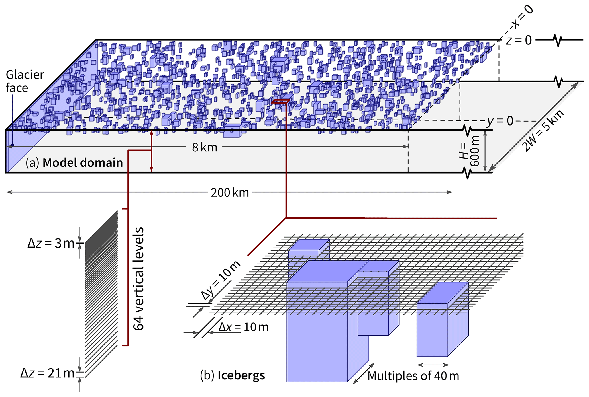
Figure 1 Numerical model setup. (a) A long rectangular fjord contains a 8 km × 5 km mélange in which 10 % of the surface area is covered by icebergs. Note the coordinate system with x=0 at the end of the mélange, y=0 in the fjord center, and z=0 at the surface. (b) Volume-occupying icebergs are explicitly resolved in the model.

The icebergs each extend over many grid cells horizontally and together act as upside-down topography (Losch, 2008). Each iceberg is assumed to be a stationary cuboid. Although there are limitations with this approach, it is their cumulative meltwater flux rather than their movement that matters most here. Further detail and justification of our approach are given by Hughes (2022).

The icebergs follow a power-law size distribution: the number of icebergs of a given horizontal area scales as A^−1.9 (Sulak et al., 2017), which means that smaller icebergs are more numerous than larger ones. Horizontally, iceberg dimensions are rounded to multiples of 40 m, and a maximum of 320 m × 240 m is imposed. Vertically, most icebergs have a keel depth of 30–80 m.

The ambient water initially has a constant potential temperature and linear salinity profile and, hence, a constant buoyancy frequency:

$$\begin{array}{}\text{(1)}& {\displaystyle }{S}_{\mathrm{a}}\left(z\right)& {\displaystyle }=\mathrm{35}-\mathrm{\Delta }S\left(\mathrm{1}+{\displaystyle \frac{z}{H}}\right),\text{(2)}& {\displaystyle }{\mathit{\theta }}_{\mathrm{a}}\left(z\right)& {\displaystyle }=\mathrm{2}\mathit{°}\mathrm{C},\text{(3)}& {\displaystyle }N& {\displaystyle }=\sqrt{g\mathit{\beta }{\displaystyle \frac{\mathrm{\Delta }S}{H}}},\end{array}$$

where ΔS=3 is the salinity increase between the surface and the seafloor, which is representative of values of 2–4 observed in Greenland fjords (e.g., Straneo et al., 2011; Sciascia et al., 2013), and $\mathit{\beta }\approx \mathrm{7.8}\times {\mathrm{10}}^{-\mathrm{4}}$ is the saline contraction coefficient. The 2 °C value equates to approximately 4 °C above freezing, an average thermal forcing for Greenland fjords (Wood et al., 2021). Constant temperature precludes local warming at mid-depths caused by upward advection of warm water (cf. Davison et al., 2022).

The coordinate system has x=0 at the end of the mélange, y=0 in the center, and z=0 at the surface. Within the mélange (x<0), $\mathrm{\Delta }x=\mathrm{\Delta }y=\mathrm{10}$ m. Outside the mélange (x>0), Δx increases by 3 % per cell. There are 64 vertical levels, with the highest resolution of Δz=3 m at the surface. The time step is 2 s, and simulations are run in hydrostatic mode for 1 week. Using nonhydrostatic simulations makes a negligible difference because – in a cumulative sense – meltwater is injected into a low-aspect-ratio layer (iceberg drafts are much smaller than the horizontal dimensions of the mélange).

Vertical mixing is parameterized with the Klymak and Legg (2010) overturning scheme with a background viscosity and diffusivity of $A_{\mathrm{v}}=K_{\mathrm{v}}=$ 10⁻⁴ m² s⁻¹. Horizontal viscosity is parameterized with a Smagorinsky viscosity with the viscC2Smag coefficient set to 2.5 together with a background value of $A_{\mathrm{h}}={\mathrm{10}}^{-\mathrm{3}}$ m² s⁻¹. Temperature and salinity are advected with a third-order flux limiter scheme (Hundsdorfer et al., 1995, designated as scheme 33 in the MITgcm).

The Coriolis parameter is set for 70° N ($f=\mathrm{1.37}\times {\mathrm{10}}^{-\mathrm{4}}$ s⁻¹). The channel width 2W=0.6L_R, where $L_{\mathrm{R}}=c_{\mathrm{1}}/f=\mathrm{8.6}$ km is the mode-1 internal Rossby radius. The mode-1 internal wave speed c₁ has a realistic value of 1.2 m s⁻¹ (e.g., Sutherland et al., 2014).

2.2 Numerical model results

The simulated icebergs melt at 0.3–0.4 m d⁻¹, which is at the upper end of typical observed values (Enderlin and Hamilton, 2014; Enderlin et al., 2018; Schild et al., 2021). This melt creates flows of order 5 cm s⁻¹ (Fig. 2). The fastest flows occur in (i) near-surface hotspots where currents are squeezed through gaps between icebergs and (ii) the coastal current down-fjord at x>20 km. This current hugging the right-hand side is the most obvious consequence of Coriolis.

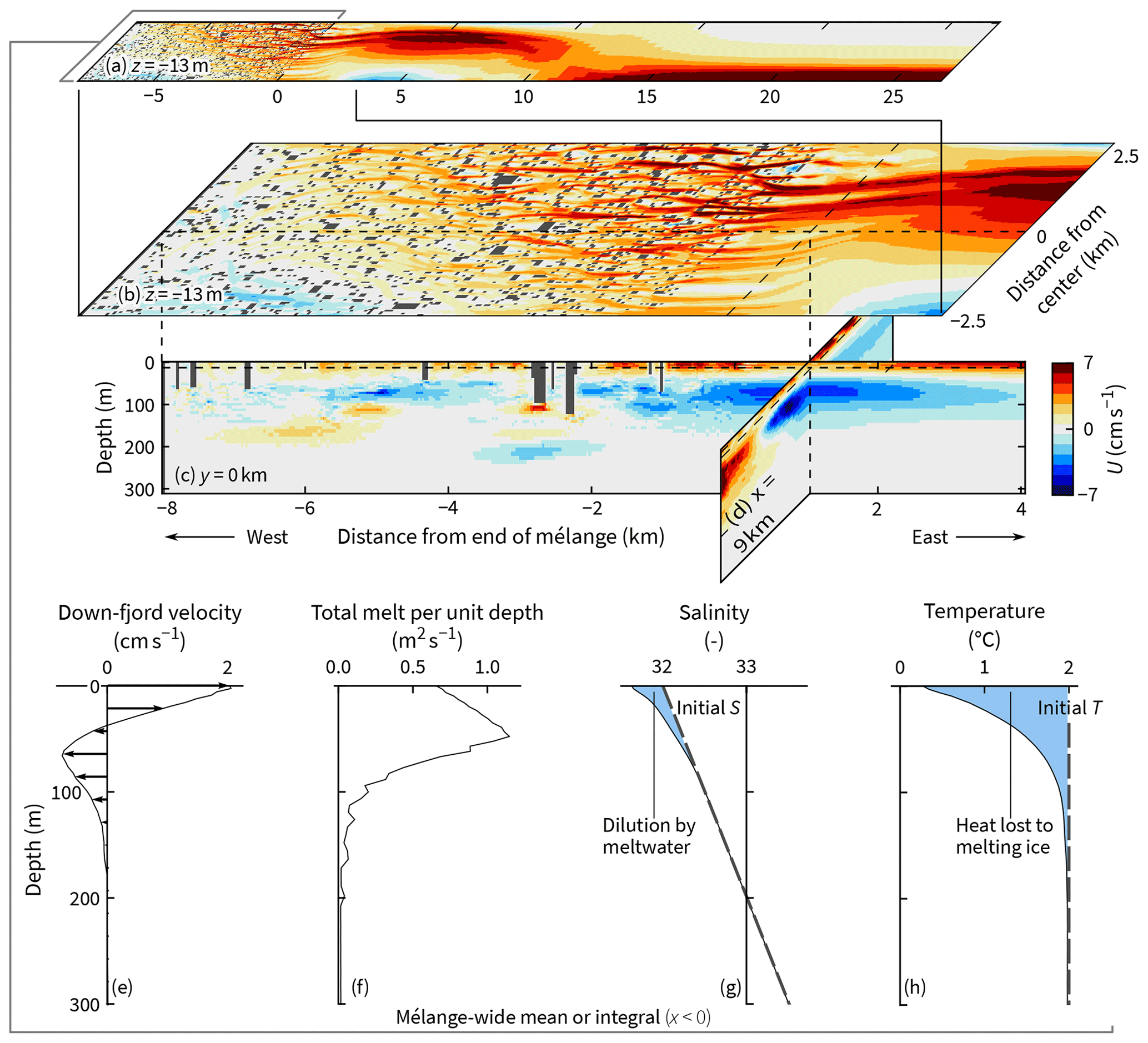
Figure 2 Dynamics of the top half of the fjord after 1 week of simulation. A simple description is of surface outflow in the top 50 m and inflow at 50–150 m, but Coriolis and advection complicate the picture. (a, b) A plan view. (c) An along-fjord slice. (d) A cross-fjord slice. (e–h) Properties averaged or integrated over the mélange region.

Most of the surface flow within the mélange is down-fjord, as expected. The up-fjord flow in the southwest corner (Fig. 2a) is perhaps not intuitive and will be explained in Sect. 3. When averaged over the whole mélange region, the outflow is down-fjord in the top 50 m and up-fjord below that (Fig. 2e). Notably, this up-fjord flow occurs despite an appreciable release of meltwater down to 100 m.

Averaged over the week-long simulation, fluxes of freshwater and heat are 110 m³ s⁻¹ and 36 TW. By the end of the week, the near-surface salinity and temperature have fallen by ∼0.3 and ∼1 °C (Fig. 2g–h).

Starting from rest, the coastal current down-fjord of the mélange is the first major feature to form (Fig. 3). As with the averaged flows described earlier, the coastal current flows down-fjord in the top 50 m and up-fjord over the 50–150 m range. Within 12 h, the current reaches x=10 km (Fig. 3b). This is too fast to be explained by advection because the currents themselves only travel at a speed of 1–3 cm s⁻¹. Instead, a faster wave mechanism is at play. This mechanism also explains why the coastal current extends over only a small fraction across the channel despite the channel width being only 0.6L_R. Specifically, the decay away from the wall is faster than $\exp (-(y+W)/L_{\mathrm{R}})$ because the current has a structure comprising many modes, not just mode 1, and the higher modes have shorter Rossby radii.

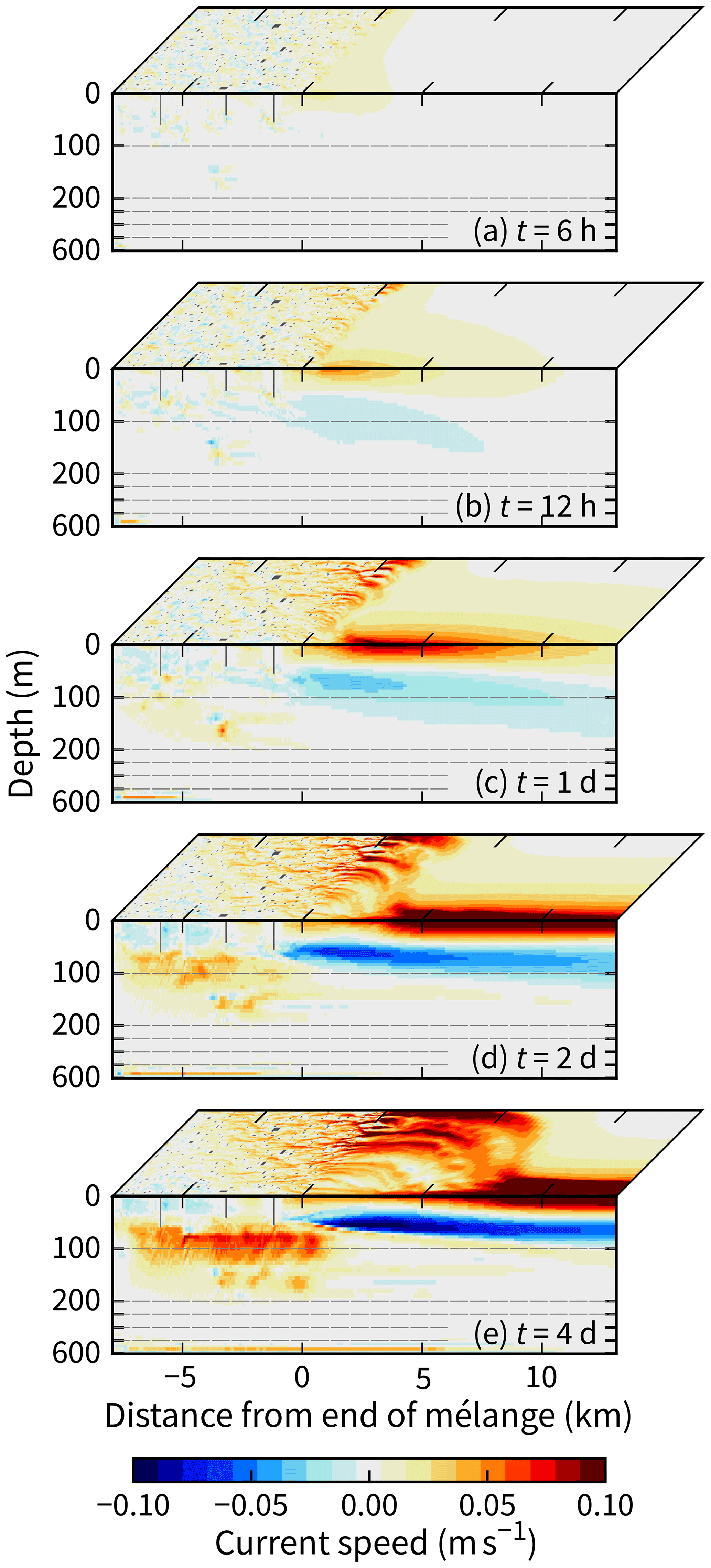
Figure 3 Development of fjord circulation from rest as depicted by vertical and horizontal slices at the southernmost side and surface, respectively ($y=-W$ and z=0). The vertical axes are enlarged in the top 200 m where currents are fastest.

Advection is responsible for the increasingly long channel-wide jet. Between t=2 and 4 d, the easternmost end of the jet moves from x=2 to 7 km (Fig. 3d–e) at 3 cm s⁻¹. However, except for this jet, the evolving system that we have simulated numerically can be explained and quantified in terms of wave mechanics with an analytical model.

3 The analytical model

We will build the core of our analytical model in nine steps (Sect. 3.1–3.9). Each step is based on wave mechanics in a certain scenario for which its section is named. The role of melt is added as a 10th step.

The first three sections consider the Rossby adjustment problem in a channel (also called geostrophic adjustment). We start with a two-dimensional problem of flow generated by an abrupt release of a region of high sea surface height in an open channel (Sect. 3.1), which is the simplest case mathematically and conceptually. We then make the geometry more realistic by closing one end (Sect. 3.2). Finally, we change the forcing for this closed case from abrupt to gradual (Sect. 3.3), which is a better analogue for a melting-ice system. Note that the term downstream in Sect. 3.1–3.3 will refer to the left of the fjord because it will simplify Fig. 4. In later sections, in which flow velocity may change sign with depth, we will use the terms up-fjord and down-fjord. Down-fjord will be to the right of the fjord.

The middle three sections consider a different two-dimensional problem: baroclinic adjustment in the x–z domain without rotation. Again, we first consider abrupt releases in open and closed settings (Sect. 3.4 and 3.5, respectively) and then look at the closed case with gradual forcing (Sect. 3.6).

The last three sections consider the three-dimensional problem with rotation. For the third time, we start with open and closed settings with abrupt releases (Sect. 3.7 and 3.8, respectively) and then the closed setting with gradual forcing (Sect. 3.9).

3.1 Barotropic, open channel, abrupt release, rotating

A sea surface height discontinuity in a fluid at rest is unbalanced. When released, the discontinuity generates waves and currents that restore equilibrium. Here, we consider this evolution toward equilibrium for a rotating, shallow-water system in a channel. The dominant signals will be Kelvin waves propagating along the boundaries and leaving behind steady boundary currents with e-folding scales equal to the Rossby radius (Poincaré waves, which have a channel-wide signature, will also arise but will be much weaker).

Consider a single discontinuity perpendicular to the channel axis (Fig. 4a). Fluid initially accelerates from higher to lower sea surface height. On a timescale of 𝒪(f⁻¹), this down-channel flow turns to the right (Northern Hemisphere) to form a cross-channel jet centered about the original discontinuity. On the wall where the jet converges, a Kelvin wave of elevation is generated; on the opposite wall, a Kelvin wave of depression is generated. Over time, these two waves propagate away and leave behind two coastal currents moving in the same direction but on opposite sides of the channel. The two currents are connected by the original cross-channel jet.

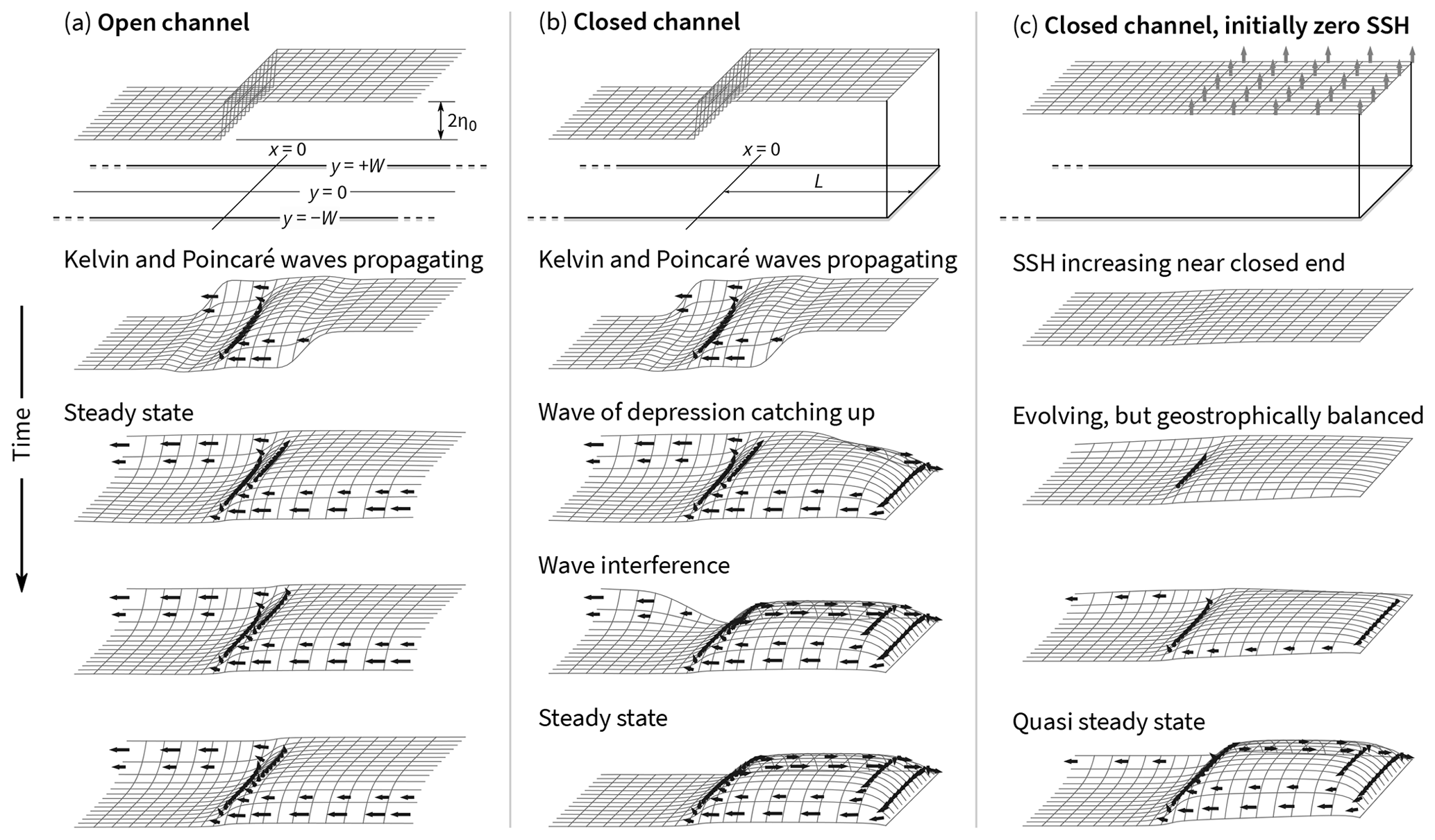
Figure 4 Rossby adjustment in a channel for three different scenarios. (a) The conventional problem with a sea surface height discontinuity in the middle of an open channel. (b) The same as panel (a) but with one end of the channel closed. (c) The same as panel (b) but with the sea surface being continually pushed upward from zero rather than having an initial discontinuity. Height anomalies are exaggerated in all panels.

Hermann et al. (1989) give analytical expressions for this wave-adjusted state (i.e., the linear solution that sets up before slower advective dynamics develop). Well downstream of the initial discontinuity (x≪0), the sea surface height η, along-channel velocity u, and total down-channel flux Q are

$$\begin{array}{}\text{(4)}& {\displaystyle }\mathit{\eta }& {\displaystyle }={\mathit{\eta }}_{\mathrm{0}}\left[\mathrm{1}-\mathrm{sech}(W/L_{\mathrm{R}})\exp (y/L_{\mathrm{R}})\right],\text{(5)}& {\displaystyle }u& {\displaystyle }={\mathit{\eta }}_{\mathrm{0}}\sqrt{g/H}\mathrm{sech}(W/L_{\mathrm{R}})\exp (y/L_{\mathrm{R}}),\text{(6)}& {\displaystyle }Q& {\displaystyle }=-\mathrm{2}{\mathit{\eta }}_{\mathrm{0}}\sqrt{gH}\tanh (W/L_{\mathrm{R}})L_{\mathrm{R}},\end{array}$$

where η₀ is the half-height of the initial surface discontinuity, W is the half-width of the channel, and H is the depth. Hermann et al. (1989) also provide expressions for u and v close to the discontinuity, but these are more elaborate and overkill for our purposes.

Evaluating Eq. (5) at the boundary gives

$$\begin{array}{}\text{(7)}& u(x\ll \mathrm{0},y=+W)={\mathit{\eta }}_{\mathrm{0}}\sqrt{g/H}(\mathrm{1}+\tanh (W/L_{\mathrm{R}}\left)\right).\end{array}$$

For an infinitely narrow channel (W→0), the tanh term goes to zero and gives the non-rotating limit. For a wide channel (W≫L_R), the tanh term goes to 1, and the maximum velocity is double the non-rotating limit. Regardless of channel width, the cross-channel integral of the change in potential energy is equal to the cross-channel integral of kinetic energy:

$$\begin{array}{}\text{(8)}& \begin{array}{rl}\int \mathrm{0.5}g(\mathit{\eta }-{\mathit{\eta }}_{\mathrm{0}}{)}^{\mathrm{2}}\mathrm{d}y& =\int \mathrm{0.5}{u}^{\mathrm{2}}H\mathrm{d}y\\ & =g{\mathit{\eta }}_{\mathrm{0}}^{\mathrm{2}}{L}_{\mathrm{R}}\tanh (W/L_{\mathrm{R}}).\end{array}\end{array}$$

3.2 Barotropic, closed channel, abrupt release, rotating

If the channel is closed on the high surface end as in Fig. 4b then the wave of depression cannot propagate toward x=∞. Instead, the wave propagates around the closed boundary and – after turning two corners – starts propagating in the same direction and on the same side of the channel as the wave of elevation. When this second wave passes back beyond x=0, it starts to cancel the effects of the first. Hence, for x<0, the down-channel flux is nonzero only between the arrival times of the two waves.

Hermann et al. (1989) did not consider this closed-channel case, but it is easy to extend their formulation (quoted here as Eqs. 4–6) by adding the destructive interference caused by the trailing wave. Assuming the trailing wave keeps its shape as it navigates the two corners, the extra distance that it travels is 2L+2W. A time series of the flux at a given location x becomes a top-hat function with nonzero values over a period Δt, where

$$\begin{array}{}\text{(9)}& \mathrm{\Delta }t=(\mathrm{2}L+\mathrm{2}W)/c.\end{array}$$

3.3 Barotropic, closed channel, gradual forcing, rotating

In Fig. 4c, there is no initial discontinuity. Instead, the sea surface is continually pushed upward in the x>0 region. This upward movement can be treated as a sum of sequential infinitesimal perturbations. Hence, the system's response can also be treated as a sum of sequential infinitesimal solutions (assuming linearity). In contrast to the abrupt closed case, $\mathit{\eta },u,$ and Q are nonzero in the x<0 region for all values of t. Expressions for these three quantities are the same as Eqs. (4)–(6) but with

$$\begin{array}{}\text{(10)}& {\mathit{\eta }}_{\mathrm{0}}\to {\displaystyle \frac{\mathrm{d}{\mathit{\eta }}_{\mathrm{0}}}{\mathrm{d}t}}\mathrm{\Delta }t,\end{array}$$

where $\mathrm{d}{\mathit{\eta }}_{\mathrm{0}}/\mathrm{d}t$ is the rate at which the sea surface is pushed upward, and Δt is the wave delay from Eq. (9).

3.4 Baroclinic, open channel, abrupt release, non-rotating

We turn now to a depth-dependent scenario: a non-rotating, open channel in two dimensions (x–z) with the left half having a low-density anomaly near the surface (Fig. 5a). In practice, the density anomaly would vary with depth as a function of meltwater input; for now, we impose a constant anomaly in the top third of the water column.

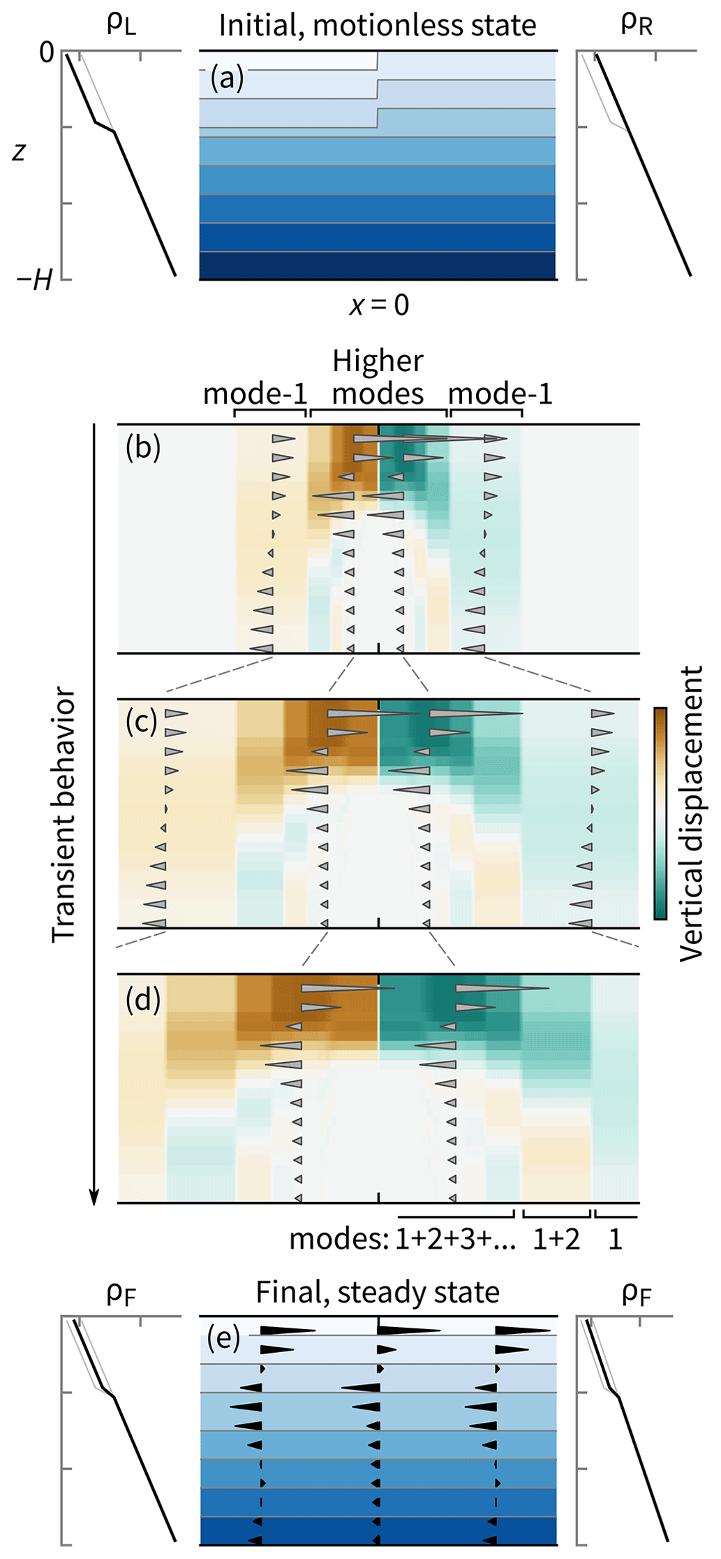
Figure 5 Baroclinic adjustment in a stratified fluid of a density anomaly near the surface of a non-rotating, open channel. (a) The initial density field. (b–d) Velocity and vertical displacement fields depicted by arrows and color shading, respectively, at three successive times. (e) The final density and velocity fields. The available potential energy in the initial, motionless state is all converted to the kinetic energy of the final, steady state. When the initial pressure anomaly is considered as a sum of internal modes, the final state – and the evolution toward it – can be predicted from the known behavior of those modes. Here, units for velocity and displacement are unimportant; only their signs and relative magnitudes matter.

The density field of the final, steady state is easy to predict. Assuming no mixing occurs, the final state must contain the same fluid parcels as the initial state but sorted vertically such that no available potential energy remains. Hence, the final density field is horizontally homogeneous (Fig. 5e).

Provided the initial density anomaly is small relative to the background stratification, it will not slump as if it were a gravity current (e.g., Simpson, 1982). Rather, each unstable fluid parcel only travels a short vertical distance before it reaches its neutral buoyancy level. Indeed, throughout this paper, we are assuming that the vertical movement of meltwater is limited by stratification, and, hence, vertical scales are a few tens of meters at most (e.g., Huppert and Turner, 1980; Yang et al., 2023).

The rearranging of fluid parcels produces pressure perturbations that lead to internal waves with a range of mode numbers spreading out in both directions from the location of the initial density discontinuity (Fig. 5b–d). For constant buoyancy frequency N and a fjord depth H, the speed of a mode-n internal wave is

$$\begin{array}{}\text{(11)}& c_n={\displaystyle \frac{NH}{n\mathit{\pi }}}.\end{array}$$

Details on this expression can be found in the Appendix of Kelly et al. (2010) or Sect. 6.11 of Gill (1982). Throughout the main text, we are using constant stratification for simplicity. The generalization of the analytical model to any stratification profile is described in Appendix B.

The two mode-1 waves spread out rapidly from the initial discontinuity. On the right-hand side, there is a wave with negative vertical displacements (green shades in Fig. 5b–d). On the left-hand side, there is a corresponding wave with positive vertical displacements. The horizontal velocity induced by these waves is the same on either side: eastward flow near the surface and westward flow deeper down. For points between the mode-1 and mode-2 wavefronts, the velocity profile is

$$\begin{array}{}\text{(12)}& u\left(z\right)=A_{u_{\mathrm{1}}}\cos \left({\displaystyle \frac{\mathit{\pi }z}{H}}\right)\text{ for }{c}_{\mathrm{2}}t<\left|x\right|<c_{\mathrm{1}}t,\end{array}$$

where $A_{u_{\mathrm{1}}}$ is a Fourier coefficient to be determined later. Once the mode-2 wavefront passes the same location, its velocity is superimposed on that already there. Hence,

$$\begin{array}{}\text{(13)}& \begin{array}{rl}& u\left(z\right)=A_{u_{\mathrm{1}}}\cos \left({\displaystyle \frac{\mathit{\pi }z}{H}}\right)+A_{u_{\mathrm{2}}}\cos \left({\displaystyle \frac{\mathrm{2}\mathit{\pi }z}{H}}\right)\\ & \text{for }{c}_{\mathrm{3}}t<\left|x\right|<c_{\mathrm{2}}t.\end{array}\end{array}$$

Similarly, the vertical displacement has both mode-1 and mode-2 components (see, e.g., the location labeled mode 1+2 in Fig. 5d).

In the long time limit, the velocity at any horizontal location is given by the generalization of Eq. (13):

$$\begin{array}{}\text{(14)}& u\left(z\right)=\sum _{n=\mathrm{1}}^{\mathrm{\infty }}{u}_n\left(z\right)=\sum _{n=\mathrm{1}}^{\mathrm{\infty }}{A}_{u_n}\cos \left({\displaystyle \frac{n\mathit{\pi }z}{H}}\right).\end{array}$$

In the example in Fig. 5, the final velocity is 17 % mode 1, 25 % mode 2, 22 % mode 3, 12 % mode 4, and 24 % higher modes.

The coefficients $A_{u_n}$ can be derived from the initial density profiles. To start, define the density anomaly ρ^′ as

$$\begin{array}{}\text{(15)}& {\mathit{\rho }}^{\prime }\left(z\right)=({\mathit{\rho }}_{\mathrm{R}}-{\mathit{\rho }}_{\mathrm{L}})/\mathrm{2},\end{array}$$

where ρ_L and ρ_R are the density profiles for the initial state on the left- and right-hand sides. Then, integrate this with depth to get a hydrostatic pressure anomaly p^′ that is the same on both the left- and right-hand sides:

$$\begin{array}{}\text{(16)}& p^{\prime }\left(z\right)={\displaystyle \frac{g}{{\mathit{\rho }}_{\mathrm{0}}}}\underset{z}{\overset{\mathrm{0}}{\int }}{\mathit{\rho }}^{\prime }\left(z^{\ast }\right)z^{\ast }\mathrm{d}{z}^{\ast },\end{array}$$

where z^∗ is a dummy variable used to avoid ambiguity with the integral's lower limit. The value of p^′(z) is zero at the surface and negative below.

Like u(z), the profile p^′(z) can be described as a cosine series:

$$\begin{array}{}\text{(17)}& p^{\prime }\left(z\right)={\displaystyle \frac{A_{p_{\mathrm{0}}}}{\mathrm{2}}}+\sum _{n=\mathrm{1}}^{\mathrm{\infty }}{A}_{p_n}\cos \left({\displaystyle \frac{n\mathit{\pi }z}{H}}\right),\end{array}$$

where

$$\begin{array}{}\text{(18)}& A_{p_n}={\displaystyle \frac{\mathrm{2}}{H}}\underset{-H}{\overset{\mathrm{0}}{\int }}{p}^{\prime }\left(z\right)\cos \left({\displaystyle \frac{n\mathit{\pi }z}{H}}\right)\mathrm{d}z.\end{array}$$

Following Kelly et al. (2010), specifically their Eqs. (A12) and (A14), with ω=0, there is a simple link between the coefficients $A_{u_n}$ and $A_{p_n}$:

$$\begin{array}{}\text{(19)}& A_{u_n}=Cn{A}_{p_n}.\end{array}$$

Therefore,

$$\begin{array}{}\text{(20)}& u\left(z\right)=C\sum _{n=\mathrm{1}}^{\mathrm{\infty }}n{A}_{p_n}\cos \left({\displaystyle \frac{n\mathit{\pi }z}{H}}\right).\end{array}$$

If ρ^′(z) is spread out with depth, then p^′(z) and u(z) are shaped more by low-mode components. If ρ^′(z) is surface intensified, then p^′ and u have higher-mode components (Fig. 6).

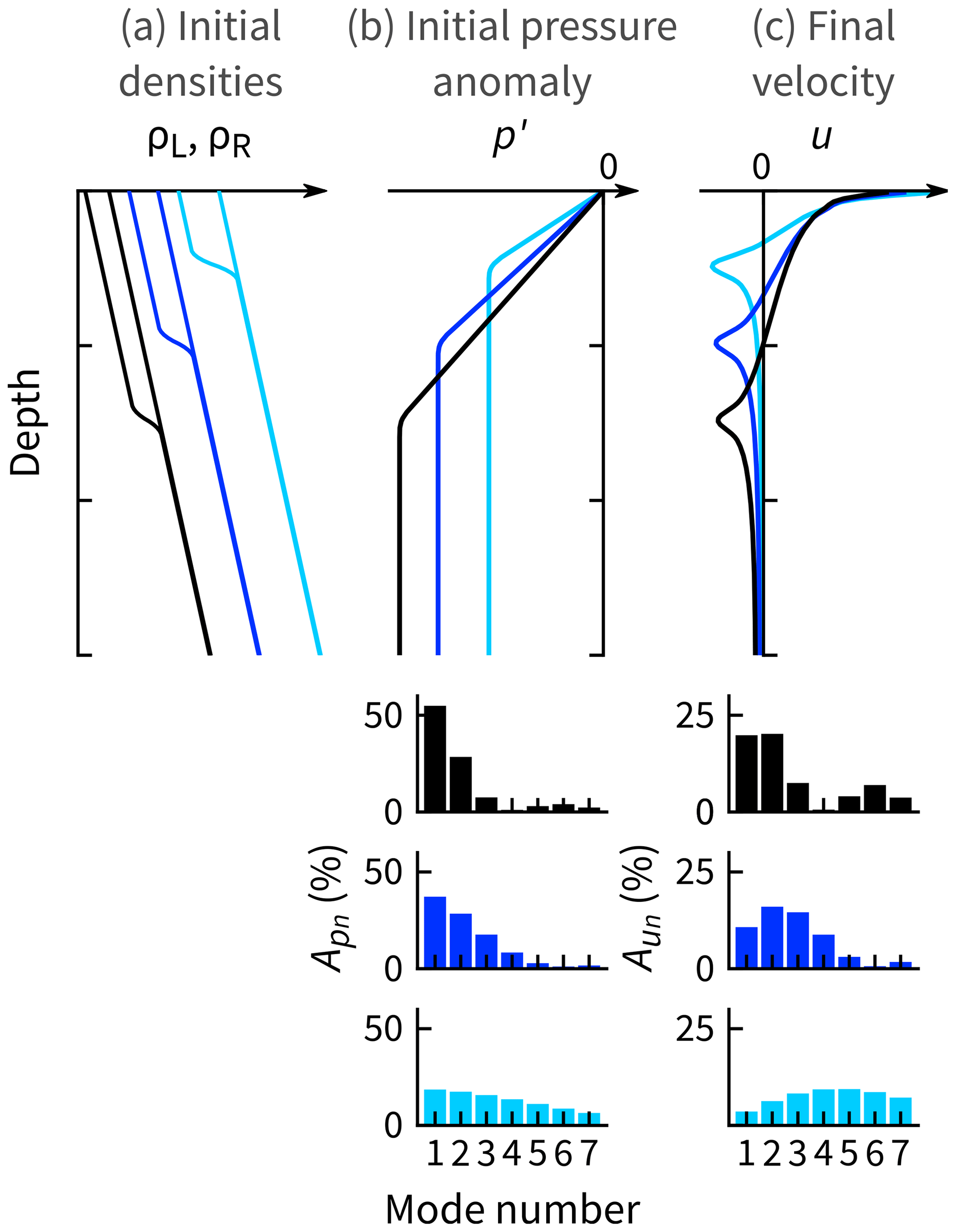
Figure 6 Examples of the link between p^′(z) and u(z) (Eqs. 14 and 17) for baroclinic adjustment of a non-rotating, stratified system. The black example has an initial density discontinuity that is most spread out with depth, so p^′(z) has lower-mode components. Hence, the associated u(z) also has lower-mode components (Eq. 19). Conversely, the light-blue example is more surface-intensified and has higher-mode components. In all cases, the initial available potential energy is the same.

The proportionality constant C in Eq. (20) is found implicitly by equating the available potential energy E_p of the initial state to the kinetic energy E_k based on the velocity in the final state u_F, where

$$\begin{array}{}\text{(21)}& {\displaystyle }{E}_{\mathrm{p}}& {\displaystyle }={\displaystyle \frac{g^{\mathrm{2}}}{\mathrm{2}{\mathit{\rho }}_{\mathrm{0}}}}\underset{-H}{\overset{\mathrm{0}}{\int }}{\displaystyle \frac{{\mathit{\rho }}^{\prime \mathrm{2}}}{N^{\mathrm{2}}}}\mathrm{d}z,\text{(22)}& {\displaystyle }{E}_{\mathrm{k}}& {\displaystyle }={\displaystyle \frac{{\mathit{\rho }}_{\mathrm{0}}}{\mathrm{2}}}\underset{-H}{\overset{\mathrm{0}}{\int }}{u}_{\mathrm{F}}^{\mathrm{2}}\mathrm{d}z.\end{array}$$

Equation (21) follows from what Kang and Fringer (2010) call APE₃. It is a good approximation here because vertical perturbations are small.

3.5 Baroclinic, closed channel, abrupt release, non-rotating

Baroclinic adjustment in a closed channel follows the same steps as for an open channel, but the boundary breaks the symmetry and means that no steady state arises. Consider the scenario in Fig. 7a of a near-surface, low-density anomaly of width L beside the closed end, where L is much smaller than the channel length. Initially, the transient behavior of the system matches that in the open-channel case in Fig. 5b: for each mode, two waves spread out from x=0. After reaching the boundary and reflecting back to x=0, the originally westward waves destructively interfere with their counterparts. Because the eastward waves had an effective head start of distance 2L, the velocity field tends toward a series of stripes, each of width 2L (Fig. 7b). The lower, faster modes are further to the right; the higher, slower modes trail behind (note the difference in presentation between Fig. 5, which shows velocities as arrows, and Fig. 7, which shows velocities with a red–blue color map).

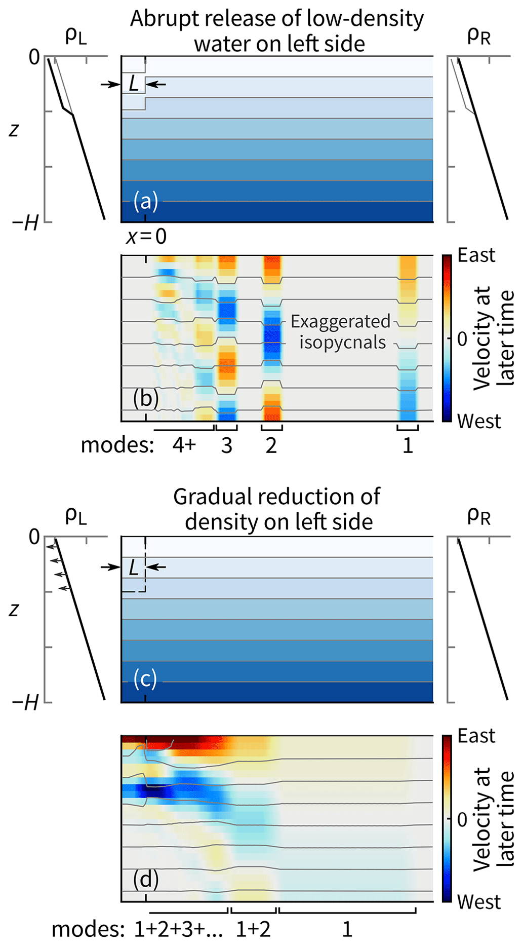
Figure 7 Baroclinic adjustment of density anomalies near the closed end of a stratified channel. (a–b) When released abruptly, the density anomaly generates two waves for each mode that spread out in each direction from x=0, just as in Fig. 5. However, the originally westward waves are reflected at the closed end and destructively interfere with the eastward waves, except for the 2L-wide portion of the waves that had a head start. (c–d) If the density anomaly is gradually built up from nothing then the outcome is the sum of sequential and infinitesimal versions of the solution in panel (b).

The potential and kinetic energy in the closed case are similar to Eqs. (21) and (22), but, due to the loss of symmetry, we must now compare Eqs. (23) and (24) below, which are the globally integrated potential energy at t=0 and the globally integrated kinetic energy as t→∞, respectively.

With our assumption that the low-density region is small compared to the channel length, the final equilibrium state can be approximated as ρ_R and not $({\mathit{\rho }}_{\mathrm{L}}+{\mathit{\rho }}_{\mathrm{R}})/\mathrm{2}$, as for the open case. Hence, the potential energy at t=0 is nonzero only in the x<0 region:

$$\begin{array}{}\text{(23)}& {\displaystyle }\underset{-L}{\overset{\mathrm{\infty }}{\int }}{E}_{\mathrm{p}}(t=\mathrm{0})\mathrm{d}x=\underset{-L}{\overset{\mathrm{0}}{\int }}{E}_{\mathrm{p}}(t=\mathrm{0})\mathrm{d}x{\displaystyle }={\displaystyle \frac{g^{\mathrm{2}}L}{{\mathit{\rho }}_{\mathrm{0}}}}\underset{-H}{\overset{\mathrm{0}}{\int }}{\displaystyle \frac{{{\mathit{\rho }}^{\prime }}^{\mathrm{2}}}{N^{\mathrm{2}}}}\mathrm{d}z.\end{array}$$

The right-hand side is Eq. (21) multiplied by 2L, where L comes from the x integration, and the factor of 2 is associated with the change to the equilibrium state for ρ. Note that ρ^′ remains as it was defined in Eq. (15).

The globally integrated kinetic energy expression involves u_n as defined in Eq. (14) and is best understood by considering Fig. 7b. That is, the total kinetic energy is the sum of all of the 2L-wide bands of nonzero velocity, each of which are a single mode provided they have had time to sufficiently spread out from each other:

$$\begin{array}{}\text{(24)}& {\displaystyle }\underset{-L}{\overset{\mathrm{\infty }}{\int }}{E}_{\mathrm{k}}(t=\mathrm{\infty })\mathrm{d}x{\displaystyle }={\mathit{\rho }}_{\mathrm{0}}L\sum _{n=\mathrm{1}}^{\mathrm{\infty }}\underset{-H}{\overset{\mathrm{0}}{\int }}{u}_n^{\mathrm{2}}\mathrm{d}z.\end{array}$$

The kinetic energy of the system increases monotonically in time and approaches Eq. (24) as t→∞.

The velocity field at any given time, depth, and position (assuming x>0) can be summarized as the total velocity induced by the eastward-propagating waves minus that of the waves that initially propagated westward and were then reflected:

$$\begin{array}{}\text{(25)}& \begin{array}{rl}u(x,z,t)& =\sum _{n=\mathrm{1}}^{n_{\mathrm{E}}}{u}_n\left(z\right)-\sum _{n=\mathrm{1}}^{n_{\mathrm{W}}}{u}_n\left(z\right)\\ & =\sum _{n=n_{\mathrm{W}}+\mathrm{1}}^{n_{\mathrm{E}}}{u}_n\left(z\right).\end{array}\end{array}$$

The integer n_E is the maximum n for which c_nt>x, and n_W is the maximum n for which $c_{n}t>x+\mathrm{2}L$.

3.6 Baroclinic, closed channel, gradual forcing, non-rotating

Consider now the same closed system but with the low-density anomaly gradually added (Fig. 7c). As in Sect. 3.3, we can treat this as a series of sequential and infinitesimal versions of the closed system that we just solved. For example, let the density everywhere be ρ_R at t=0, and let the left side be reduced at a constant rate of $({\mathit{\rho }}_{\mathrm{L}}-{\mathit{\rho }}_{\mathrm{R}})/\mathit{\tau }$. In other words, τ is the time it would take for the left-hand side to reach ρ_L if the system were held in place so that it could not respond.

If we want to know the velocity field at any time t then we sum a large number m (e.g., 100) of solutions to the abrupt-release, closed case (Eq. 25) that are evenly spaced in time up until t. Specifically,

$$\begin{array}{}\text{(26)}& u(x,y,z,t)=\sum _{i=\mathrm{1}}^{m}u(x,y,z,it/m),\end{array}$$

with the effective ρ_L being reduced accordingly:

$$\begin{array}{}\text{(27)}& {\mathit{\rho }}_{\mathrm{L}}\to {\mathit{\rho }}_{\mathrm{R}}-{\displaystyle \frac{t}{m\mathit{\tau }}}\left({\mathit{\rho }}_{\mathrm{R}}-{\mathit{\rho }}_{\mathrm{L}}\right).\end{array}$$

For example, if m=100 then we effectively sum 100 abrupt-release cases that start at $\mathrm{0.00}t,\mathrm{0.01}t,\mathrm{0.02}t,\mathrm{\dots },\mathrm{0.99}t$, with each having values of ρ_R−ρ_L that are scaled down by a factor of 100. Although we could also express this more formally in the limit m→∞, doing so does not provide extra insight.

With this gradual release in a stratified channel, we can start to see a resemblance between the analytical and numerical models (e.g., compare Fig. 7d to 3c).

3.7 Baroclinic, open channel, abrupt release, rotating

Three-dimensional baroclinic Rossby adjustment in a channel combines concepts from the x–y and x–z cases from Sect. 3.1–3.6. We will use the same initial density field as in Sect. 3.4–3.6 and make it constant in the across-channel direction (Fig. 8a).

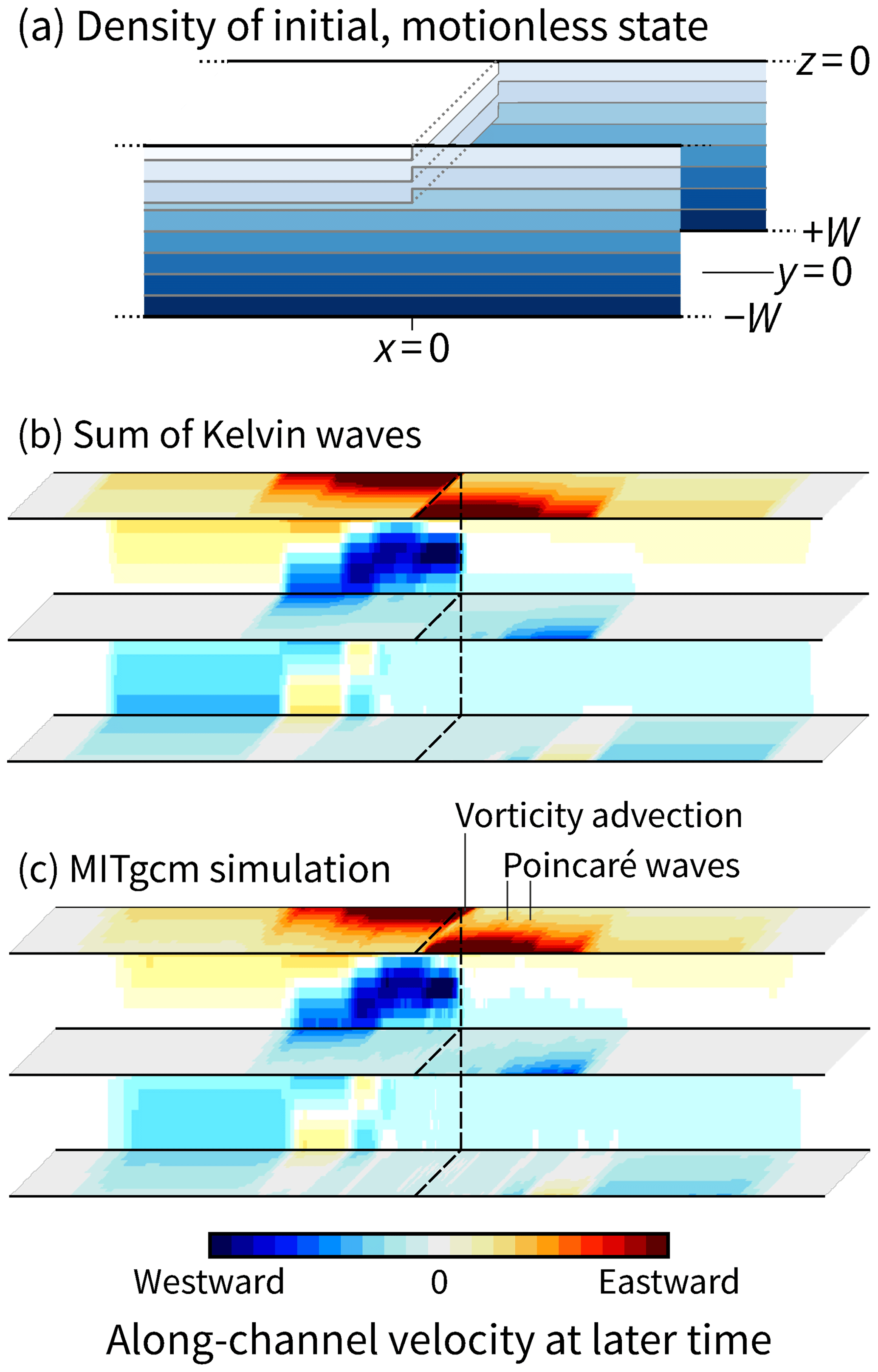
Figure 8 Baroclinic Rossby adjustment in an open-ended, stratified channel predicted by analytical and numerical models. The values of velocity are unimportant here, but the initial densities and the color maps for panels (b) and (c) are identical. The MITgcm simulation shows two slight additions that do not arise with a semi-geostrophic approximation: advection of the discontinuity and Poincaré waves. For this particular example, the channel width is equal to the mode-1 internal Rossby radius.

When the density discontinuity is released, it generates two counter-propagating families of Kelvin waves (Fig. 8b): westward ones on the far side of the channel ($y=+W$) and eastward ones on the closer side ($y=-W$), just as occurred in the simpler form with barotropic waves in Fig. 4a. Individually, each mode behaves like the barotropic case, except with a depth-dependent velocity and a much reduced Rossby radius. The latter for a given mode n is

$$\begin{array}{}\text{(28)}& L_{\mathrm{R}n}={\displaystyle \frac{NH}{n\mathit{\pi }f}},\end{array}$$

which follows from the wave speed expression in Eq. (11). Mode-1 Rossby radii are typically 5–10 km in Greenland fjords.

For regions away from the initial discontinuity, the velocity is parallel to the walls, and the expression for $u(x,y,z,t)$ is separable in three dimensions. In x and z, we use the two-dimensional baroclinic solution from Sect. 3.4. In y, velocities decay exponentially and follow the scaling in Eq. (5). More specifically, the velocity field is

$$\begin{array}{}\text{(29)}& \begin{array}{rl}u(x,y,z,t)& =\sum _{n=\mathrm{1}}^{n_{\mathrm{E}}}{A}_{u_n}\cos \left({\displaystyle \frac{n\mathit{\pi }z}{H}}\right)\\ & \cdot \mathrm{sech}(W/L_{\mathrm{R}n})\exp (-\mathrm{sgn}(x)y/L_{\mathrm{R}n}),\end{array}\end{array}$$

where $A_{u_n}$ are the velocity coefficients derived for the non-rotating x–z solution, and n_E is defined as in Sect. 3.5.

A curious consequence of the superposition in Eq. (29) is that, at certain points, u does not decay monotonically away from the boundary. Instead, the differing scales and phases of the individual modes can lead to local maxima or minima in u(y) within the channel. However, a clear example of this does not arise in Fig. 8b.

To confirm that the sum of Kelvin waves is a good approximation of the true system, we test it against an MITgcm simulation with the same initial conditions (this simulation is separate to those described in Sects. 2 and 4). In Fig. 8, panels (b) and (c) clearly agree, and the same is true for wider and narrower channels (not shown). The MITgcm simulation does contain additional physics, namely vorticity advection and Poincaré waves, but the effect on along-channel velocity is small (see Hutter et al., 2011, for further details on Poincaré waves in channels of constant depth).

Not shown in Fig. 8 are the cross-channel velocities. It would be possible, albeit cumbersome, to derive $v(x,y,z,t)$ from linear wave dynamics as we have done for $u(x,y,t,z)$; the starting point would be the solution for the barotropic case (Eq. 2.22 of Hermann et al., 1989). From the MITgcm simulations, we find, as expected, that v (not shown) peaks near x=0, goes to zero at $\left|x\right|\gg \mathrm{0}$, and is negative at the surface: water flows from $y=+W$ to −W. A counterflow from −W to +W occurs at the depth $z=-H/\mathrm{3}$, where the discontinuity goes to zero.

3.8 Baroclinic, closed channel, abrupt release, rotating

In a closed channel, the baroclinic Kelvin waves propagating toward the closed end start at $(x,y)=(\mathrm{0},+W)$, travel a distance L westward, turn a corner, travel a distance 2W southward, turn another corner, and travel a distance L eastward to arrive at (0, −W). Thereafter, they destructively interfere with their counterparts. This is the same argument as in the barotropic case in Sect. 3.2. Ultimately, Eq. (25) can be applied here to the three-dimensional channel, with n_W now being the maximum value of n for which $c_{n}t>x+\mathrm{2}L+\mathrm{2}W$.

3.9 Baroclinic, closed channel, gradual forcing, rotating

The final step before incorporating melt is anticlimactic because the hard work has been done. To adapt the closed, abrupt-release case from the previous section to the gradual-release case, we simply repeat the methodology described by Eqs. (26) and (27).

3.10 Incorporating ice melt into the analytical model

In Sect. 3.4–3.9, there is a low-density anomaly in the upper third of the water column in the x<0 region that either exists at t=0 or develops gradually as t increases. The numerical model from Sect. 2 is set up similarly in that meltwater is continually injected into the x<0 region.

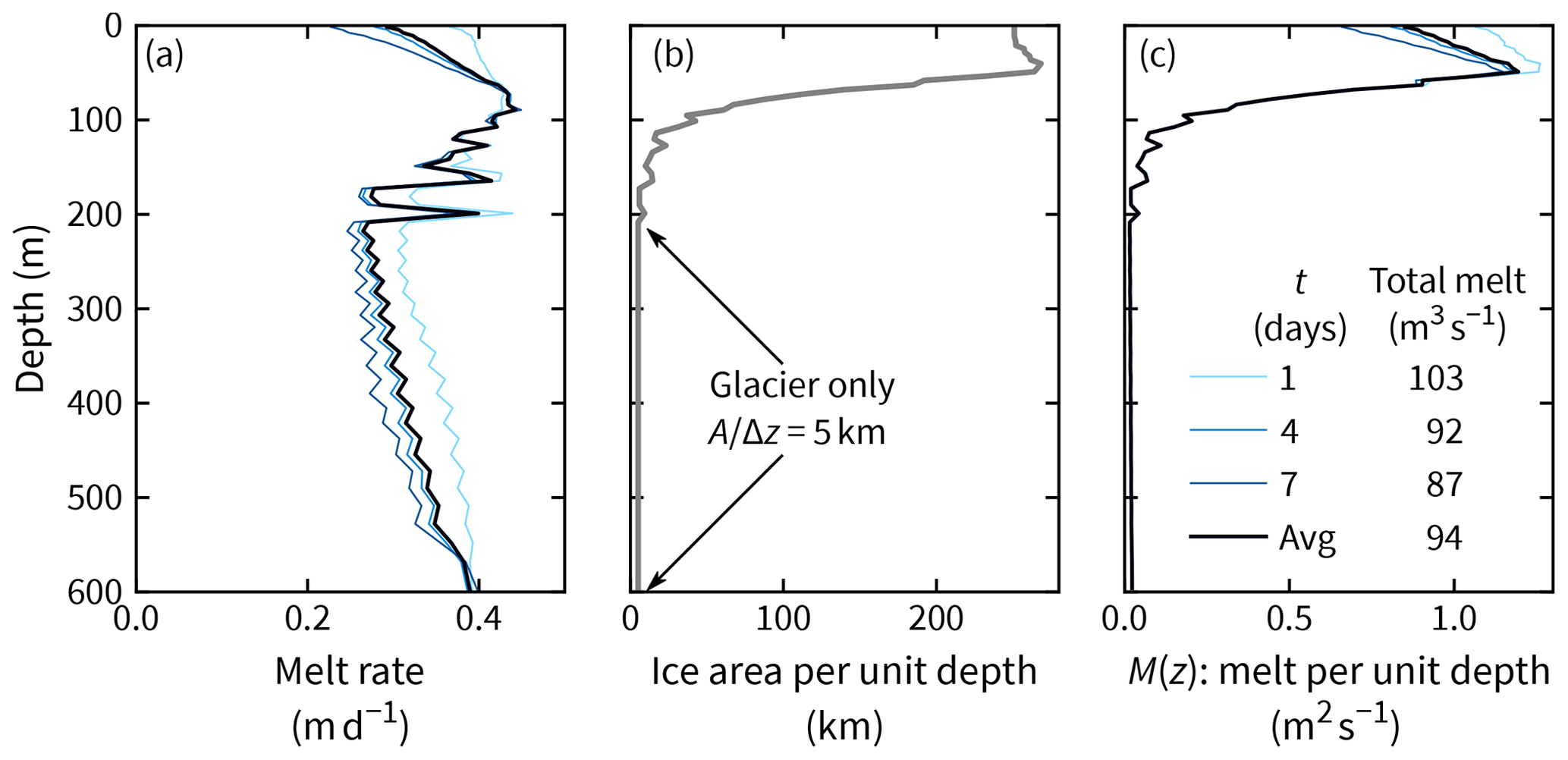
Figure 9 Iceberg (and glacier) melt in the numerical model. (a) Melt rates are ∼0.3 m d⁻¹ and decrease over time, especially near the surface, as the surrounding water cools. (b) Total ice surface area in units equivalent to a width. (c) The product of panels (a) and (b) in units that are suitable for the analytical model.

In a glacier context, melt rates are often discussed in velocity units, with a convenient unit being meters per day (m d⁻¹) as in Fig. 9a. In iceberg-choked fjords, the total surface area of ice in contact with water can be 1 order of magnitude larger (Sulak et al., 2017). Indeed, expressing this surface area per unit depth gives a quantity that is equivalent to a glacier's width but much bigger, especially near the surface (e.g, ∼200 km in Fig. 9b).

Let M(z) denote the total, time-averaged meltwater input per unit depth with units of meters squared per second (m² s⁻¹) (the depth integral of M(z) is the volume flux of meltwater). Many remote sensing studies provide methods to estimate M(z) from either observed rates of change of iceberg freeboard or parameterizations of melting (Enderlin and Hamilton, 2014; Enderlin et al., 2018; Moon et al., 2018; Moyer et al., 2019; Rezvanbehbahani et al., 2020). We, however, have the benefit of the exact value of M(z) being a model output, so we will use this hereafter (Fig. 9c).

To use the analytical model, we need an expression for ρ_L(z) that plugs into Eq. (27). We start with meltwater's properties (see, e.g., Jenkins, 1999):

$$\begin{array}{}\text{(30)}& {\displaystyle }S& {\displaystyle }=\mathrm{0},\text{(31)}& {\displaystyle }{\mathit{\theta }}_{\mathrm{eff}}& {\displaystyle }\approx -{\displaystyle \frac{L}{c}}+{\displaystyle \frac{c_{\mathrm{i}}}{c}}{\mathit{\theta }}_{\mathrm{i}},\end{array}$$

where θ_eff is the effective potential temperature of meltwater; θ_i is the ice temperature; L is the latent heat of fusion; and c_i and c are the specific heat capacities of ice and water, respectively. The value of θ_eff is approximately −85°C and is dominated by the first term, which accounts for the heat extracted from the water to induce the phase change; the second term accounts for sensible heating of the ice to its freezing point.

In Sect. 3.6, we defined the profile ρ_L together with the timescale τ that defined how long it took for the left side to be reduced from ρ_R to ρ_L at a constant rate. Here, we set a somewhat arbitrary value for τ of 7 d and calculate ρ_L at this time based on the meltwater input. The value of τ later cancels when used in Eq. (27).

At time τ, the volume of meltwater per unit depth added over the mélange will have reached ΔA(z)=M(z)τ. If the fjord did not respond dynamically to this meltwater then the average properties throughout the mélange region – based on weighted averages of the ambient water and meltwater – would become

$$\begin{array}{}\text{(32)}& {\displaystyle }{S}_{\mathrm{L}}& {\displaystyle }={\displaystyle \frac{A_{\mathrm{0}}{S}_{\mathrm{R}}}{A_{\mathrm{0}}+\mathrm{\Delta }A}},\text{(33)}& {\displaystyle }{\mathit{\theta }}_{\mathrm{L}}& {\displaystyle }={\displaystyle \frac{A_{\mathrm{0}}{\mathit{\theta }}_{\mathrm{R}}+\mathrm{\Delta }A{\mathit{\theta }}_{\mathrm{eff}}}{A_{\mathrm{0}}+\mathrm{\Delta }A}},\text{(34)}& {\displaystyle }{\mathit{\rho }}_{\mathrm{L}}& {\displaystyle }=\mathit{\rho }(S_{\mathrm{L}},{\mathit{\theta }}_{\mathrm{L}}),\end{array}$$

where S_R and θ_R are the initial salinity and potential temperature profiles, and A₀(z)=2WLϕ(z) is the mélange area scaled by the water fraction ϕ(z). In our numerical model, we have ϕ=0.9 at the surface because 10 % of the surface is covered by icebergs.

4 Comparing the analytical and numerical models

The analytical model should work in regions governed by linear wave dynamics; it is not expected to work where advection dominates (e.g., at x≲15 km in Fig. 2a). We will start by testing it at x=20 km by comparing its prediction to the numerical model from Sect. 2.

Consider first the cross-channel structure. At t=1 d, the analytical model correctly predicts that the flow (i) has peak velocities of 1 cm s⁻¹, (ii) has a zero-crossing at 100 m depth, and (iii) has a decay scale comparable to the width of the channel (Fig. 10a–b). Also correctly predicted, albeit a minor detail, is the small outflowing patch centered near 350 m depth. Later, at t=3 and 7 d (Fig. 10c–f), there is a larger contribution from higher modes, and the flows are consequently more concentrated in the top 100 m. The analytical model still predicts well the velocity fields at both of these times.

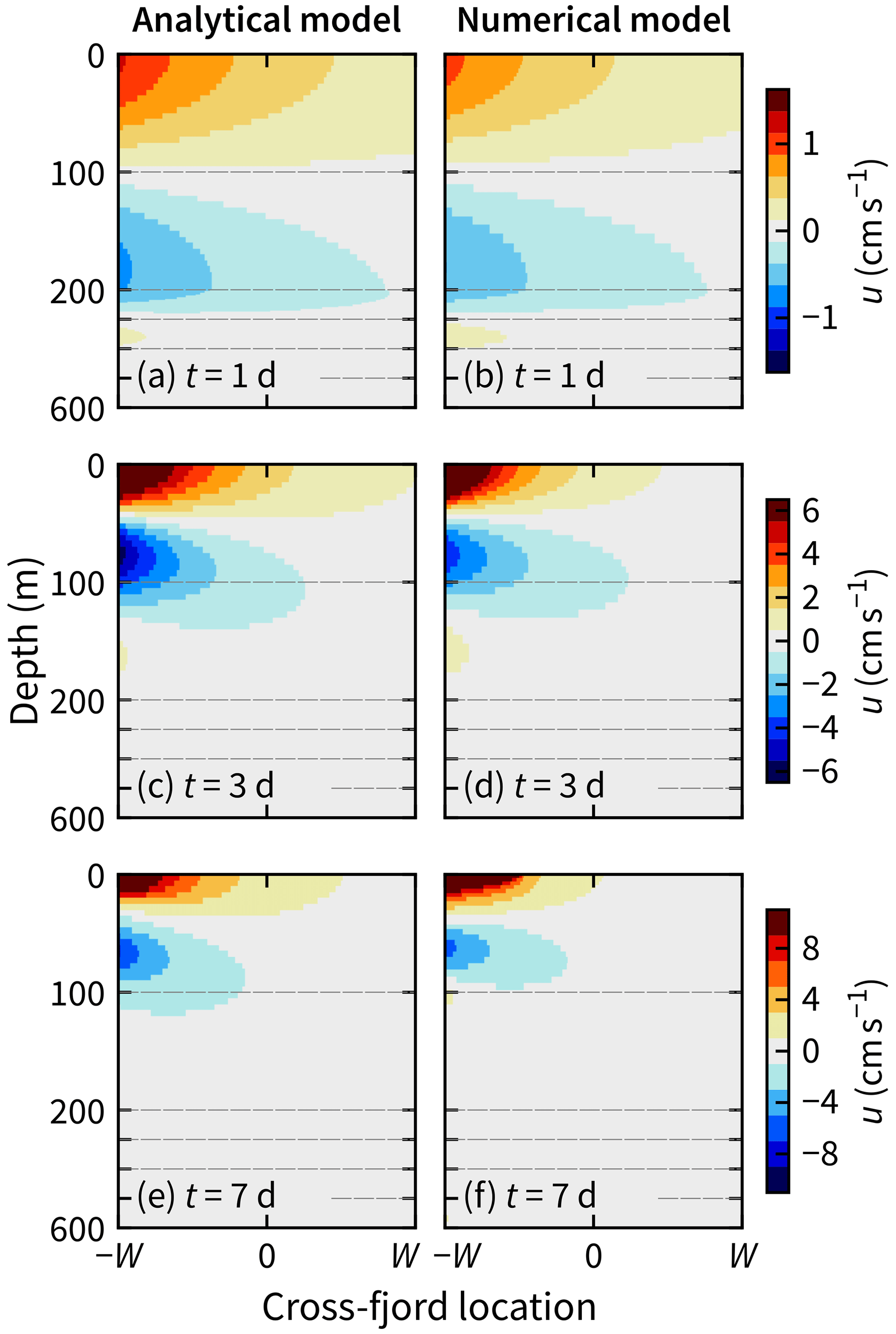
Figure 10 Snapshots at x=20 km after 1, 3, and 7 d show that the analytical predictions in the left column agree with the numerically simulated velocities in the right column. Note that the color limits increase from the top to bottom and that the vertical axes are enlarged in the top 200 m as in Fig. 3.

When compared carefully, the analytical model slightly overpredicts the velocities. This is best quantified by evaluating the total outflow Q_out, which is the area integral of all outflowing fluid:

$$\begin{array}{}\text{(35)}& Q_{\mathrm{out}}=\underset{u>\mathrm{0}}{\int }u\mathrm{d}y\mathrm{d}z.\end{array}$$

Between 3 and 7 d (once a quasi-steady state is approached), the analytical model overpredicts Q_out at x=20 km by 25 % (compare the gray and black lines in Fig. 11a). At t=7 d, the analytical model predicts that Q_out is approximately independent of distance from the mélange – at least for x<100 km (Fig. 11b). The same approximate independence arises in the numerical model results, except in the aforementioned advective region of x<15 km.

Given the number of approximations and assumptions that go into the analytical model, we deem it to be that it agrees reasonably well with the numerical model. One notable assumption not yet discussed is that the icebergs have no dynamical effect as obstacles. In the numerical model, the icebergs are stationary and induce drag on near-surface flows (Hughes, 2022), which includes the set of Kelvin waves that initially travel westward from x=0 and then counterclockwise around the fjord boundary.

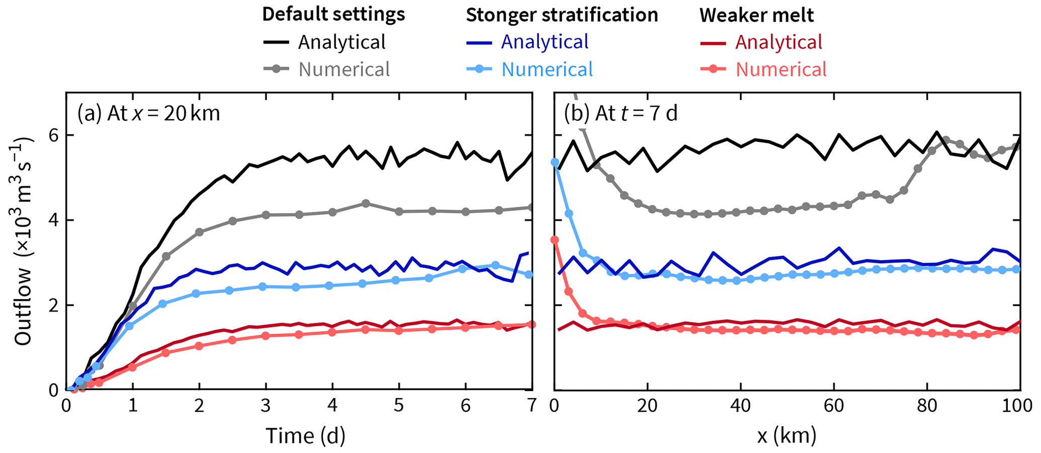
Figure 11 The analytical model predicts the outflow well (Eq. 35) for three different scenarios. (a) Outflow at a specific location: 20 km. (b) Outflow at a specific time: 7 d. The discrepancies are discussed in the main text.

To further test the analytical model, we repeat the Q_out comparisons for two other model scenarios. The first scenario has stronger stratification: the salinity difference between the surface and seafloor is doubled (ΔS in Eq. (1) is 6 and not 3). The second scenario has weaker melt rates: the turbulent-transfer coefficients for heat and salt are 4 times smaller than the default case (γ_T and γ_S in Eqs. A3 and A4). In these two further tests, the analytical model still predicts well the numerically simulated flow both in terms of total outflow (Fig. 11) and cross-channel structure (not shown). In fact, the agreement is better in these two scenarios compared to the default settings because the relative role of linear wave dynamics (compared to nonlinear advection) is larger when the outflow is weaker or the stratification is stronger.

Three comparisons are, of course, far from an exhaustive test of the plausible parameter space. Yet, given the agreement in all cases, there is no reason not to trust the analytical model.

5 Discussion

5.1 What parameters does melt-induced circulation depend on?

There are several obvious ways that melt-induced fjord circulation could increase: warmer ambient water, a larger mélange, or enhanced turbulent transfer at the ice–ocean interface.

To examine these dependencies – and the less intuitive role of stratification – in detail, we undertake a parameter space study using the analytical model to predict Q_out(x=20 km) under a range of conditions. For simplicity, we will change one parameter at a time; all others will have the default values used previously (L=8000 m, 2W=5000 m, H=600 m, ΔS=3, and θ_a=2°C). We will also assume a total melt rate profile similar to that in Fig. 9c. Specifically,

$$\begin{array}{}\text{(36)}& M\left(z\right)=\mathrm{2.5}\times {\mathrm{10}}^{-\mathrm{8}}WL\left(\mathrm{1}+\tanh \left({\displaystyle \frac{z+\mathrm{100}}{\mathrm{25}}}\right)\right),\end{array}$$

where 100 m is the depth at which M(z) drops to half of its surface maximum, and 25 m is a vertical length scale. For the default fjord geometry, $M(z=\mathrm{0})=\mathrm{1}$ m² s⁻¹.

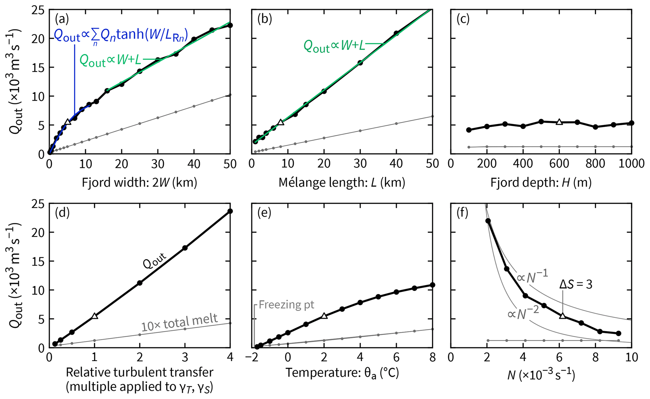
Figure 12 Predictions from the analytical model of how outflow (Q_out) depends on geometrical parameters, ice–ocean turbulent transfer, and water column properties. In each panel, a single quantity is varied; the others are fixed at the values highlighted by the triangles in the other five panels. Note how the total meltwater flux, which is shown for reference, is multiplied by a factor of 10 to make it visible on the same scale.

Q_out increases monotonically with channel width (Fig. 12a). For narrower channels, there is a dependence on ${\sum }_n{Q}_n\tanh (W/L_{\mathrm{R}n})$, where Q_n are coefficients. This follows from generalizing Eq. (6) to the baroclinic case involving a sum of modes, each with their own internal Rossby radius L_Rn (presumably the coefficients Q_n could be derived from the analytical model, but that is not our goal here). For wider channels, $Q_{\mathrm{out}}\propto W+L$ because the distance 2L+2W is the distance a Kelvin wave travels around the perimeter of the fjord to move from $(\mathrm{0},+W)$ to $(\mathrm{0},-W)$, and this distance governs the total flux (see Sect. 3.2 and 3.8). For the same reason, a $Q_{\mathrm{out}}\propto W+L$ scaling also arises when varying L while keeping W constant (Fig. 12b). The other geometrical parameter – fjord depth H – has no significant effect on Q_out (Fig. 12c).

If the fjord geometry is fixed but the ice–ocean interface conditions are changed then Q_out scales approximately linearly with the meltwater flux. In Fig. 12d, we alter the ice–ocean turbulent-transfer coefficients γ_T and γ_S (see Appendix A). In Fig. 12e, we alter the ambient temperature. In both cases, linearity dominates; slight deviations from this arise from nonlinearities in the equation of state and the melt rate derived from the three-equation formulation. Note, however, that, for this analysis, we assumed a fixed ambient velocity of 0.04 m s⁻¹ (see Appendix A). Different melt formulations (e.g., Greisman, 1979; Magorrian and Wells, 2016; Malyarenko et al., 2020) may lead to different dependencies for Q_out, but we do not investigate these here.

Q_out vs. water column stratification N is the scaling that needs the most steps to be explained. First, recall the open-channel, non-rotating system from Sect. 3.4. There, u and, hence, Q_out are $\propto N^{-\mathrm{1}}$ because $E_{\mathrm{p}}=E_{\mathrm{k}}\propto N^{-\mathrm{2}}$ (Eq. 21). However, $Q_{\mathrm{out}}\propto N^{-\mathrm{2}}$ for the equivalent closed, gradual-release system (Sect. 3.6). The additional factor of N⁻¹ arises because the internal wave speed c∝N (Eq. 11). Specifically, recall Fig. 7, in which the gradual-release case was described as the sum of sequential versions of the abrupt-release case, with the latter consisting of 2L-wide bands of nonzero velocity. These bands move and separate at a rate ∝N, and so the magnitude of their sum is $\propto N^{-\mathrm{1}}$. This already elaborate explanation is further complicated by rotation because the internal Rossby radii $L_{\mathrm{R}n}=c_n/f\propto N/n$. With increasing L_Rn, flow occupies a wider portion of the channel, and, hence, Q_out increases. Ultimately, in the full system, Q_out has a scaling that tends to fall between N⁻¹ and N⁻² (Fig. 12f).

All panels in Fig. 12 include a line showing the total meltwater flux. In many cases, Q_out is ∼50 times larger than the meltwater flux, but in some cases, the ratio is as large as 200 (small L or small N) or as small as 20 (large W or large N).

5.2 The value of simple scaling laws in Greenland fjords

An ambitious goal for our analytical model would be to make large-scale predictions like those that exist for the role of subglacial discharge. These start with classic buoyant-plume theory (Morton et al., 1956), which is extended to a salinity-stratified system and then applied at a large scale. For example, Slater et al. (2016) show that outflow in a fjord is proportional to $Q_{\mathrm{sg}}^{\mathrm{3}/\mathrm{4}}/N^{\mathrm{5}/\mathrm{8}}$, where Q_sg is the subglacial discharge rate. Slater et al. (2022) apply this scaling to more than 100 fjords around Greenland to predict that a total of 20 000 m³ s⁻¹ of meltwater discharge gets amplified by a factor of ∼50 due to entrainment and that the outflow is spread over the top ∼200 m.

A more immediate goal is to help interpret observations or numerical models for specific settings. For example, as part of ongoing related work, we are analyzing multi-year simulations of Sermilik Fjord with and without icebergs (using a setup like Davison et al. (2020) but with seasonal variability included). Iceberg effects are isolated by looking at the difference between the two simulations. One plausible but counter-intuitive hypothesis stemming from the analytical model is that melt-induced circulation will be larger in winter than in summer. Why? Because in winter the water column is less stratified (hence larger iceberg-melt-induced outflow), and this may overcome the effect of slower melting in cooler waters.

5.3 Next steps

The analytical model is built on linear wave dynamics; nonlinear advection and instabilities are ignored. In parts of the domain, this can quickly become a limitation. In the numerical model, we saw advection dominating in the $\mathrm{0}<x<\mathrm{10}$ km region after only 1 week of spin-up (Fig. 2a). In principle, it may be possible to extend the analytical model to predict this advective component. The approach would follow Hermann et al. (1989), from whom we borrowed the analytical expressions for the barotropic wave-adjusted state in Sect. 3.1. For Hermann et al. (1989), the wave-adjusted state was merely the starting point for predicting the slower advective dynamics. In the baroclinic setting, however, the math would quickly become cumbersome.

Instead, it makes more sense to simply ask whether the analytical model would remain skillful after several months. Without running simulations to properly answer this, our best guess follows from Carroll et al. (2017), who simulated circulation induced by subglacial discharge on timescales of months. Their Figs. 2 and 3 imply that spin-up of the linear circulation (i.e., boundary currents) happens within the first 5 d. Thereafter, eddies form via instabilities and advection, especially in the wider channels. Nevertheless, their outflow metric seems mostly unaffected by these nonlinearities.

Other obvious uncertainties surround whether the analytical model still works in fjords that feature sills or have realistic coastlines, whether it remains useful in the presence of competing forcings such as shelf waves and subglacial discharge, and how it should be adapted for the case where there is not a convenient demarcation of mélange and open water but rather where iceberg concentration varies along the fjord.

6 Conclusion

The analytical model involved many steps. A summarizing example helps bring all of these steps together.

The continual input of meltwater generates a continual fjord response. Discretizing the problem in time makes this response easier to understand. In Fig. 13, we divide the problem into 100 pieces: 1 % of the meltwater is released at t=0.00t₀, another 1 % is released at t=0.01t₀, and so on up to t=0.99t₀. The circulation at t=t₀ is the sum of these (Fig. 13b).

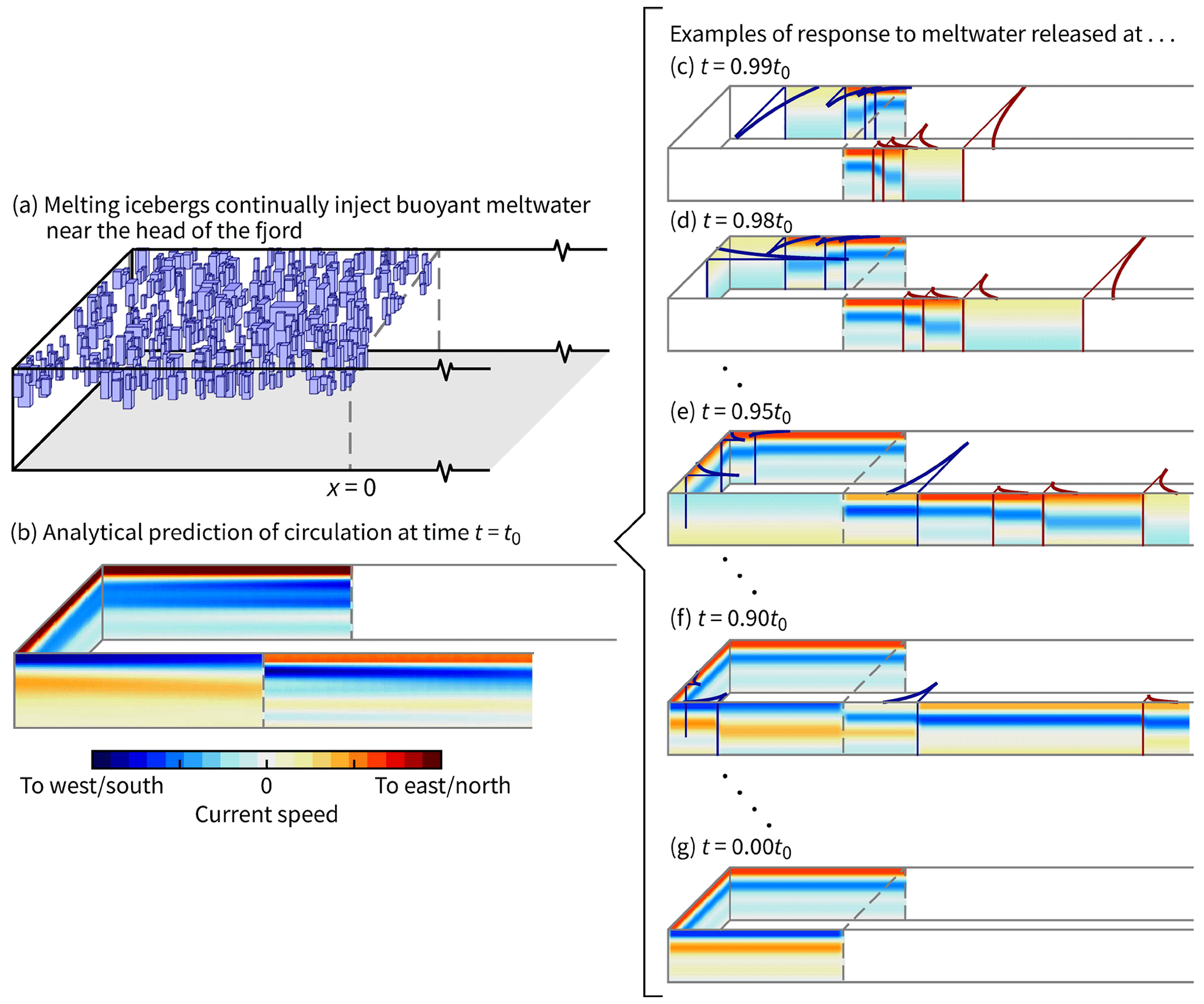
Figure 13 Summary of the analytical model. To predict the total fjord circulation at a given time t=t₀ as in panel (b), we approximate the continual forcing as, say, 100 sequential, abrupt-release cases, examples of which are shown in panels (c)–(g). See Sect. 6 for a complete description. For clarity, velocities are shown only at the fjord edges, and only the lowest four modes are considered. Color scales in panels (c)–(g) are the same, but they are different to that in panel (b).

For the response to the last 1 % released at t=0.99t₀, we see the lower modes move away quickly from x=0, with the higher modes trailing behind (Fig. 13c). In front of the mode-1 wavefronts on each side of the fjord, velocities are zero. Behind the mode-1 wavefronts, but in front of the mode-2 wavefronts, the velocities are down-fjord in the top half and up-fjord in the bottom half. These velocities decay exponentially from the wall, but, being mode 1, they extend to a reasonable distance. Wavefronts for the higher modes trail behind, and their associated velocities decay rapidly with distance from the wall. The same general velocity structure is present for the case with meltwater released at t=0.98t₀, except that the mode-1 wavefront on the far side has turned the corner (Fig. 13d).

For the t=0.95t₀ case (Fig. 13e), the mode-1 wave that originated on the far side travels around the fjord perimeter and starts to interfere with the velocity field generated by the other set of Kelvin waves. The mode-2 wave does the same in the t=0.90t₀ case (Fig. 13f). With enough time, this interference occurs for all modes. Indeed, for the t=0.00t₀ case, the velocity field shown in Fig. 13g is zero for x>0. This motionless region therefore has no influence on the total velocity field in Fig. 13b.

Figure 13 implicitly illustrates that, down-fjord of x=0, melt-induced fjord circulation reaches a quasi-steady state in which it only responds to the “recent” input of meltwater, with the term recent being linked to the time it takes for the relevant modes (say modes 1 through 10) to travel around the boundary. For most Greenland fjords, this will be only a few days.

Ultimately, the analytical model – and the scalings that follow from it (Sect. 5.2) – can help to tame the daunting problem of predicting the dynamics of fjords that are subject to numerous forcings, of which iceberg melt is only one. Of course, there is still much to do in extending this analytical model to one that is directly applicable to a realistic fjord. But we have taken the first steps to predicting flows induced by iceberg melt that could be applied to fjords across Greenland.

Appendix A: Ice–ocean thermodynamics

In our simulations, icebergs produce meltwater through only subsurface melting; wave erosion and melting at the ice–air interfaces are ignored. Thermodynamics at all ice–ocean interfaces are treated with the three-equation formulation, and the same velocity-dependent turbulent-transfer coefficients are used for the vertical sides and the basal face. Specifically, we adapt the “icefront” package implementation from Xu et al. (2012). Turbulent heat fluxes to the ice–ocean interface are

$$\begin{array}{}\text{(A1)}& {\displaystyle }\text{heat transfer }\left(\mathrm{W}{\mathrm{m}}^{-\mathrm{2}}\right)& {\displaystyle }=\mathit{\rho }{c}_{\mathrm{p}}{\mathit{\gamma }}_T\left|\mathbf{u}\right|\mathrm{\Delta }T,\text{(A2)}& {\displaystyle }\text{salt transfer }\left(\mathrm{m}{\mathrm{s}}^{-\mathrm{1}}\right)& {\displaystyle }={\mathit{\gamma }}_S\left|\mathbf{u}\right|\mathrm{\Delta }S,\end{array}$$

where ΔT is the difference between the temperature at the ice–ocean interface and the temperature in the adjacent ocean cell, and this is similarly the case for ΔS. The interface conditions come from the solution to the three-equation formulation. The transfer coefficients for heat and salt (in units of m s⁻¹) are ${\mathit{\gamma }}_T\left|\mathbf{u}\right|$ and ${\mathit{\gamma }}_S\left|\mathbf{u}\right|$, where

$$\begin{array}{}\text{(A3)}& {\displaystyle }{\mathit{\gamma }}_T& {\displaystyle }=\mathrm{4.4}\times {\mathrm{10}}^{-\mathrm{3}},\text{(A4)}& {\displaystyle }{\mathit{\gamma }}_S& {\displaystyle }=\mathrm{1.24}\times {\mathrm{10}}^{-\mathrm{4}},\text{(A5)}& {\displaystyle }\left|\mathbf{u}\right|& {\displaystyle }=\min \left(\sqrt{u^{\mathrm{2}}+v^{\mathrm{2}}+w^{\mathrm{2}}},\mathrm{0.04}\mathrm{m}{\mathrm{s}}^{-\mathrm{1}}\right).\end{array}$$

The values of γ_T and γ_S are far from well constrained; the decimal places are shown only to help preserve a link to previous studies that used ${\mathit{\gamma }}_T=\mathrm{1.1}\times {\mathrm{10}}^{-\mathrm{3}}$ and ${\mathit{\gamma }}_S=\mathrm{3.1}\times {\mathrm{10}}^{-\mathrm{5}}$ (e.g., Xu et al., 2012; Sciascia et al., 2013). Observations suggest these values are too low at vertical or near-vertical ice faces in Greenland (Jackson et al., 2020; Schulz et al., 2022). We have increased γ_T and γ_S by a factor of 4 following the suggestion of Jackson et al. (2020, 2022)¹ based on their scenario in which a resolved horizontal velocity is incorporated into the calculation of the transfer coefficients (rather than just vertical velocity). In our case, $\left|\mathbf{u}\right|$ values are calculated in the cells adjacent to ice–water interfaces. At each interface, two of the three velocity components will be nonzero. For example, v≠0 and w≠0 for an ice face in the y–z plane. The 0.04 m s⁻¹ lower limit follows Slater et al. (2015) and is intended to represent unresolved melt-driven convection.

Appendix B: Extension to arbitrary stratification

Conceptually, the analytical model does not change if the reference density is nonlinear. The only difference is that mode shapes and internal wave speeds need to be calculated numerically with matrix methods.

Mode shapes for vertical velocity, denoted ${\mathit{\varphi }}_n^w$, are the eigenvectors of the following equation:

$$\begin{array}{}\text{(B1)}& {\displaystyle \frac{{\partial }^{\mathrm{2}}}{\partial z^{\mathrm{2}}}}{\mathit{\varphi }}_n^w+{\displaystyle \frac{N^{\mathrm{2}}}{c_n^{\mathrm{2}}}}{\mathit{\varphi }}_n^w=\mathrm{0},\end{array}$$

with boundary conditions requiring that ${\mathit{\varphi }}_n^w=\mathrm{0}$ at the surface and seafloor. The internal wave speeds c_n are derived from the eigenvalues. We are interested in the horizontal velocity mode shapes, which we denote as ϕ_n without a superscript:

$$\begin{array}{}\text{(B2)}& {\mathit{\varphi }}_n={\displaystyle \frac{\partial {\mathit{\varphi }}_n^w}{\partial z}}.\end{array}$$

It is easy to confirm that ${\mathit{\varphi }}_n=\cos (n\mathit{\pi }z/H)$ and $c_n=NH/n\mathit{\pi }$ are eigensolutions to the above set of equations if N is constant. Extending the analytical model to nonlinear stratification simply involves replacing all appearances of $\cos (n\mathit{\pi }z/H)$ and $NH/n\mathit{\pi }$ with ϕ_n and c_n, respectively.