the Creative Commons Attribution 4.0 License.
the Creative Commons Attribution 4.0 License.
 | 19 Mar 2024
Lead fractions from SAR-derived sea ice divergence during MOSAiC
Luisa von Albedyll
Stefan Hendricks
Nils Hutter
Dmitrii Murashkin
Lars Kaleschke
Sascha Willmes
Linda Thielke
Xiangshan Tian-Kunze
Gunnar Spreen
Christian Haas
Leads and fractures in sea ice play a crucial role in the heat and gas exchange between the ocean and atmosphere, impacting atmospheric, ecological, and oceanic processes. We estimated lead fractions from high-resolution divergence obtained from satellite synthetic aperture radar (SAR) data and evaluated them against existing lead products. We derived two new lead fraction products from divergence with a spatial resolution of 700 m calculated from daily Sentinel-1 images. For the first lead product, we advected and accumulated the lead fractions of individual time instances. With those accumulated divergence-derived lead fractions, we comprehensively described the presence of up to 10 d old leads and analyzed their deformation history. For the second lead product, we used only divergence pixels that were identified as part of linear kinematic features (LKFs). Both new lead products accurately captured the formation of new leads with widths of up to a few hundred meters. We presented a Lagrangian time series of the divergence-based lead fractions along the drift of the Multidisciplinary drifting Observatory for the Study of Arctic Climate (MOSAiC) expedition in the central Arctic Ocean during winter 2019–2020. Lead activity was high in fall and spring, consistent with wind forcing and ice pack consolidation. At larger scales of 50–150 km around the MOSAiC expedition, lead activity on all scales was similar, but differences emerged at smaller scales (10 km). We compared our lead products with six others from satellite and airborne sources, including classified SAR, thermal infrared, microwave radiometer, and altimeter data. We found that the mean lead fractions varied by 1 order of magnitude across different lead products due to different physical lead and sea ice properties observed by the sensors and methodological factors such as spatial resolution. Thus, the choice of lead product should align with the specific application.
- Article
(8738 KB) - Full-text XML
- BibTeX
- EndNote


Divergent motion in sea ice leaves open water in the sea ice cover, which we refer to as fractures or leads. These openings play a crucial role in the polar climate system, altering atmospheric, ecological, and oceanic processes. In winter, the exchange of gases and heat between the ocean and atmosphere is strongly enhanced at the openings in the ice in the otherwise well-separated components of the polar climate system (Maykut, 1978, 1982; Perovich, 2011). Turbulent heat is transferred from the ocean to the atmosphere, followed by rapid new ice formation and brine rejection to the ocean during winter. The enhanced exchange has important implications. First, new ice formation in leads contributes about 30 % to the Arctic sea ice mass balance and the thin ice influences the sea ice dynamics (von Albedyll et al., 2022; Kwok, 2006). Second, they enable ocean–atmosphere gas exchange: for instance, water vapor, iodine, and methane relevant in Arctic cloud formation (e.g., Leck et al., 2002; Kort et al., 2012; Dall'Osto et al., 2017; Saavedra Garfias et al., 2023). Third, they may act as sources of atmospheric sea salt from frost flowers growing on ice-covered leads (e.g., Perovich and Richter-Menge, 1994; Kaleschke et al., 2004; Hara et al., 2017). Fourth, in summer, their low albedo increases solar transmission to the ocean. Fifth, they act as important hunting grounds for marine mammals, and sixth, they are important shipping routes (e.g., Massom, 1988; Stirling, 1997). In addition, leads are easily detectable signs of sea ice deformation, and studying their occurrence, spacing, orientation, intersection, and scale invariance is of great relevance for sea ice mechanics (e.g., Weiss and Marsan, 2004; Hutter et al., 2019; Hutter and Losch, 2020; Ringeisen et al., 2023). Lastly, leads are important for remote sensing of sea ice thickness by satellite altimetry as the method relies on lead detections to measure the instantaneous sea surface height for ice freeboard retrieval (e.g., Laxon et al., 2003).
The distribution of leads follows the overall dynamic regimes of the Arctic Ocean. While the lead frequency, i.e., how often a lead is found at a certain position within a certain time period, is a few percent for the central Arctic Ocean, it can rise to over 40 % in the Barents and Kara seas and the marginal ice zone (Willmes and Heinemann, 2016; Reiser et al., 2020). Although leads cover only 1 %–3 % of the sea ice area (Wadhams, 2000; Reiser et al., 2020), their impact on the winter heat budget is significant (Maykut, 1978; Marcq and Weiss, 2012): An increase of 1 % in lead fraction can increase the near-surface temperatures in the Arctic by 3.5 K under clear-sky conditions during polar night (Lüpkes et al., 2008).
Due to their high relevance for the polar climate, accurate knowledge of the location and areal fraction of leads (“lead fraction”) is crucial for understanding and modeling processes at the air–ocean interface, but also the global weather and climate (Serreze et al., 2009). This is particularly interesting considering that Arctic sea ice drift and deformation rates are increasing (e.g., Rampal et al., 2009; Spreen et al., 2011), with an unclear impact on the changes in lead fractions. Consequently, the importance of leads for the sea ice mass balance has gained increased attention in recent sea ice modeling studies (e.g., Wilchinsky et al., 2015; Zhang et al., 2021; Ólason et al., 2021; Boutin et al., 2023), as well as using lead statistics to evaluate different rheological frameworks for sea ice dynamics (Wang et al., 2016; Hutter and Losch, 2020; Hutter et al., 2022). In contrast to the transient nature of leads, they can have a long deformation history as the ice breaks preferentially where it is thinner than the surrounding ice (e.g., Wilchinsky and Feltham, 2011). In other words, leads can undergo several cycles of opening, closing, and ridging, interrupted by dormant phases ranging from days to months. However, there is a general lack of high-resolution reference datasets available for evaluating the magnitude, temporal and spatial variability, and deformation history of leads.
Satellites have monitored the spatial distribution and temporal evolution of Arctic lead fraction since the 1990s (Key et al., 1993; Lindsay and Rothrock, 1995; Miles and Barry, 1998). Lead detection based on thermal infrared (TIR, Willmes and Heinemann, 2016; Hoffman et al., 2022; Wang et al., 2022; Qiu et al., 2023) and visible images (e.g., Lewis and Hutchings, 2019; Muchow et al., 2021) was complemented by classification of synthetic aperture radar (SAR) backscatter (e.g., Murashkin et al., 2018), radar altimeters (e.g., CryoSat-2 Hendricks et al., 2021a), laser altimeters (e.g., ICESat-2 Duncan and Farrell, 2022), and passive microwave (PMW) data (e.g., Röhrs et al., 2012). The transient nature of leads and their narrow appearance set limits to the detection of leads from satellites. Most retrieval methods suffer either from a low spatial resolution (e.g., PMW), low spatial coverage (e.g., altimeters), low temporal coverage due to clouds or the absence of daylight (e.g., TIR and visible), or ambiguous classification due to acquisition geometry (e.g., SAR). In addition, the definition of a lead is ambiguous as it can be covered by open water or thin ice of up to 30 cm thickness (new and young ice according to the World Meteorological Organization, 2014). However, the different lead identification methods do not have a clear boundary when the ice gets too thick to be classified as a lead. This results in inconsistent estimates of the lead fraction between the retrieval methods that can vary by magnitudes. So far, there have only been a few comparison studies between lead products, which concluded that the compared products often show similar spatiotemporal patterns but vary substantially in magnitude (Kwok, 2002; Lee et al., 2018).
In lead fraction retrievals, little focus has been placed on deriving lead fractions from their driving mechanism, i.e., the divergent motion of the ice floes (Kwok, 2002). The sea ice divergence of the sea ice velocity is directly linked to lead fraction and can be calculated from high-resolution sea ice drift. Kwok (2002) demonstrated the technique using RADARSAT Geophysical Processor System (RGPS) data in the Pacific sector of the Arctic with a 3 d temporal resolution. So far, the low temporal resolution of SAR images has hindered a more area-wide application, but this has changed in recent years with the start of the Sentinel-1 constellation and many other SAR missions. This growing availability of SAR images in the polar region motivates us to explore the potential of divergence derived from SAR data for estimating lead fraction. More precisely, here we present a novel lead fraction dataset based on data from the Sentinel-1 constellation.
The interdisciplinary Multidisciplinary drifting Observatory for the Study of Arctic Climate (MOSAiC) expedition took place between October 2019 and September 2020 in the transpolar drift on board the R/V Polarstern (Nicolaus et al., 2022; Rabe et al., 2022; Shupe et al., 2022). We have selected the MOSAiC expedition as our study case for several reasons. First, the drift covered a wide range of different dynamic regimes (Krumpen et al., 2021). Second, there are important complementary atmospheric and ocean datasets and regional, high-resolution, airborne observations of leads available. Third, leads were a cross-cutting theme for all MOSAiC disciplines, i.e., ice, ocean, atmosphere, ecology, and biogeochemistry, and a sound estimate of regional lead fractions is crucial for their research (Nicolaus et al., 2022; Rabe et al., 2022; Shupe et al., 2022).
This study has two objectives. First, we present and evaluate two novel lead products that are based on SAR-derived sea ice divergence. To do so, we compare the novel lead products with six already existing lead products. Second, we present and analyze a time series of lead fractions along the MOSAiC drift track based on the novel and existing datasets. As most lead products are only available in wintertime, we restrict our analysis to October 2019 to May 2020.
The structure of the study is as follows: in Sect. 2, we describe the physical properties of leads used to detect them and introduce the novel lead products along with the existing ones participating in the comparison. Section 3 presents the properties of the lead products based on divergence including basic statistics of the observed leads and a time series on different spatial scales. Section 4 analyzes the temporal and spatial differences between the novel and existing lead products. The concluding sections, Sects. 5–6, discuss and summarize the results and outline potential improvements.
What is a lead? Each lead fraction retrieval method gives a different answer to this question. Depending on the application and the research question behind it, the underlying lead definition of a lead product may have advantages or restrictions. Therefore, we start this section with a description of the physical properties of a lead (Sect. 2.1) and explain how the different retrieval methods make use of them (Sects. 2.2–2.3).
2.1 Physical properties of a lead detected by remote sensing
The World Meteorological Organization (WMO) defines a lead as a “fracture or passage-way through sea ice which is navigable by surface vessels” whereby fractures are defined as “break[s] or rupture[s] through very close ice, compact ice, consolidated ice […] resulting from deformation processes. Fractures may contain brash ice and/or be covered with nilas and/or young ice” (World Meteorological Organization, 2014). Following this definition, a lead can be covered by up to 30 cm (young ice) thick ice (World Meteorological Organization, 2014). In this study, and almost everywhere else in the literature, fractures and leads are often summarized under the term “leads”, and their minimum width and maximum ice thickness depend on the sensitivity of the retrieval method. However, this sensitivity, especially with respect to the maximum lead ice thickness, is often not precisely known.
Figure 1 provides an overview of the physical properties that are exploited to detect leads from space. We outline the properties and link them to the retrieval methods introduced in Sect. 2.2–2.3.
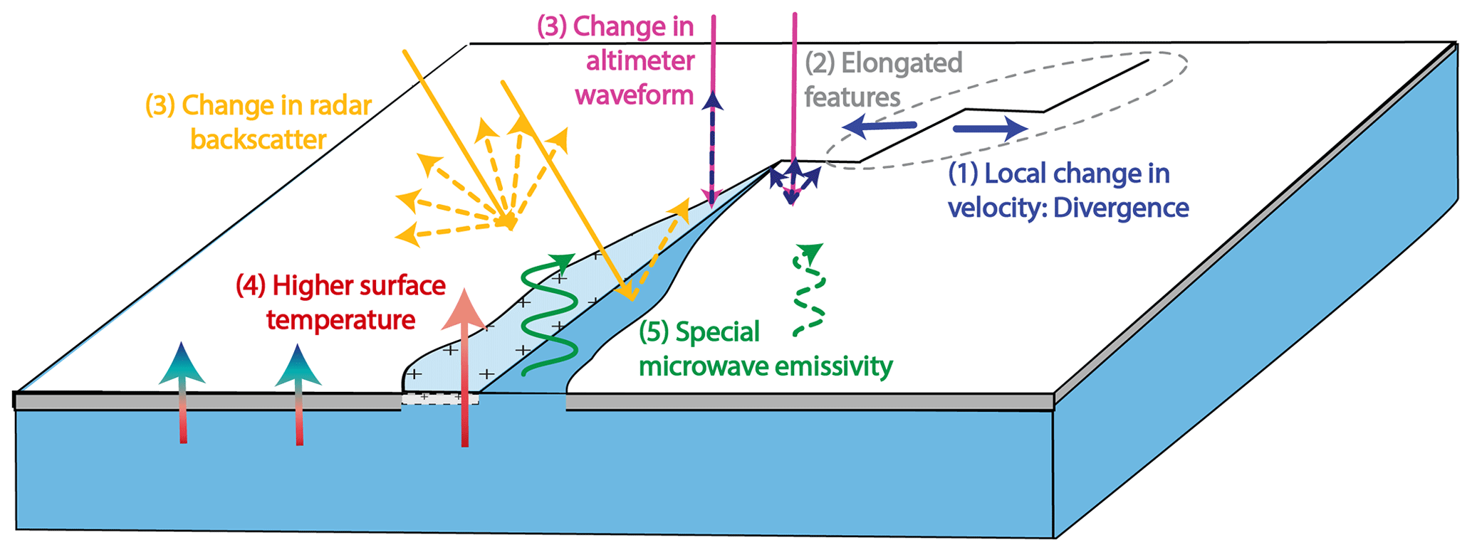
Figure 1Schematics of different physical properties of a lead detected by remote sensing instruments. Leads can be open water (blue) or covered with thin ice (light blue and crosses). Numbers refer to the subsections of Sect. 2.1 discussing the properties. The abrupt change in surface properties (roughness, salinity, surface temperature, and surface height probability distribution) in a lead affects the interaction of the surface with microwaves, thus modulating the radar backscatter (yellow) and the altimeter waveform (pink, Sect. 2.1.3).
2.1.1 Local change in ice velocity
Leads result from deformation processes and their creation can be detected by a strong local gradient in the ice velocity. External drivers, mainly winds and ocean currents, induce stress on sea ice. Sea ice breaks when those stresses reach the ice strength, resulting in deformation (for an overview see Weiss, 2013). Breaking, followed by divergent ice motion, forms leads and the divergence magnitude is directly proportional to the lead width. The two novel lead fraction products based on divergence exploit this property to detect leads (Sect. 2.2.1–2.2.2).
2.1.2 Elongated features
Leads typically have an elongated shape with a long extent in one direction (length) and a very small extent in the other direction (width). In the absence of coastlines, they can appear in systems of parallel faults of the order of several kilometers to 1000 km (Goldstein et al., 2000). More generally speaking, including ridges, shear zones, and leads, these narrow lines where deformation concentrates are called linear kinematic features (LKFs). Several lead fraction products use this property to create a shape-based noise filter (Sect. 2.2.2, 2.3.1, 2.3.2, 2.3.4).
2.1.3 Abrupt change in surface properties
Leads have very different surface properties than the surrounding ice with respect to the roughness, salinity, surface temperature, and surface height probability distribution function. The scattering and absorption of radar (microwave) waves depend strongly on those parameters, and therefore leads typically provide a strong contrast to the surrounding sea ice surface. For example, leads with calm open water or thin ice are specular scatter targets (low radar backscatter) in contrast to sea ice surfaces with more diffuse scatter (high backscatter). Leads with waves or frost flowers appear very rough, especially when using radar with a wavelength in the range of a few centimeters like Sentinel-1 (5.5 cm wavelength), and thus have higher backscatter than the surrounding ice. Therefore, lead classifications of SAR data can detect open water and leads covered with thin ice depending on the backscatter statistics (lower or higher than the backscatter of the surrounding sea ice, Sect. 2.3.1). The abrupt change in the surface properties also modifies the shape of the altimeter radar waveforms in a characteristic way which is used to detect leads by, e.g., CryoSat-2 (e.g., Wernecke and Kaleschke, 2015; Paul et al., 2018, Sect. 2.3.5). In optical remote sensing, leads appear darker due to specular reflection on the smoother surface and light transmission through the thin ice into the open water. However, visible images are not included in this study because we focus on the wintertime and high latitudes, where no sunlight is available.
2.1.4 Higher surface temperature
In winter, the ocean temperature in leads is at the freezing point close to −1.8 °C, while the surrounding ice and snow surface approach much colder air temperatures, resulting in temperature differences of −10 to −40 °C. This temperature contrast is clearly seen in the TIR part of the EM spectrum and recorded by helicopter-borne (Sect. 2.3.3) or spaceborne instruments (MODIS, Sect. 2.3.2). When new ice starts to form in the open water, the surface temperature anomaly in leads gradually decreases.
2.1.5 Special microwave emissivity
Thin ice has a special emissivity in the microwave spectrum. Comparing the emissivity at different frequencies and polarizations allows us to detect open water and thin ice. While the polarization difference is highest for open water, leads covered with thin ice exhibit a particularly high emissivity at 89 GHz with vertical polarization (Eppler et al., 1992). Lead fractions based on PMW data exploit this characteristic (Sect. 2.3.4).
2.1.6 Local thickness and surface elevation minimum
Leads are characterized by open water or thin ice and thus exhibit a local minimum in the ice thickness and surface elevation. When the lead is not closed by convergent dynamics, this difference to the surrounding ice can persist. However, there is no agreed-upon maximum thickness for considering the thin ice to be a lead. Thresholds in different studies range between open water and 1 m (Wadhams, 2000). In this study, we only use the criterion of a local surface elevation minimum to define leads in the complementary airborne ice thickness observations (Sect. 2.3.6). However, some sensors predominantly make use of the surface elevation minimum to detect leads, e.g., the laser altimeter ICESat-2.
2.2 Novel lead products based on SAR-derived sea ice divergence
In this section, we present two new lead products. Both are based on divergence in the sea ice motion that is derived from SAR data with a spatial resolution of 50 m. The divergence indicates the exact location of the lead, is independent of clouds, and, as noted by Kwok (2002), is independent of sensor calibrations and physical understanding of the radar backscatter signal of the ice.
While Kwok (2006) has previously used this general concept, we present two products that have a much higher temporal and spatial resolution, are regularly gridded, are advected and accumulated over several days, and are evaluated extensively with other lead products and a complementary airborne ice thickness dataset. The first lead product is based solely on the divergence, while the second product first derives LKFs from the total deformation before indicating the presence of leads.
2.2.1 Accumulated divergence-derived lead fractions (LFaccu. div)
Our first novel lead product is directly derived from the divergence fields that are calculated following von Albedyll et al. (2021a). The divergence-derived lead fractions (LFdiv) detect the strong, local change in ice velocity (Sect. 2.1.1).
Calculating lead fractions from divergence consists of three steps. First, we derive sea ice drift and deformation fields. We use sequential SAR scenes in HH polarization extra-wide swath mode obtained by the Sentinel-1 mission (ESA) with a spatial resolution of 50 m (Torres et al., 2012). The scenes were acquired along the drift track of the MOSAiC expedition, are centered around R/V Polarstern, and typically have a side length of 200–400 km. We aim for a nominal time difference of 1 d between the scenes but accept everything between 0.9 and 3 d. The lower limit of 0.9 d is chosen to guarantee a displacement larger than the uncertainty of the tracking. Images are available for the entire study period from October 2019 to May 2020, except for the time between 14 January and 15 March 2020, when the ship was north of the latitudinal limit of Sentinel-1. We use a tracking algorithm based on Thomas et al. (2008, 2011) and substantially extended by Hollands and Dierking (2011) to derive sea ice drift. Next, we calculate the spatial derivatives from the regularly spaced drift field following von Albedyll et al. (2021a). Divergence and convergence are then derived from the spatial derivatives of the velocity field (u,v).
Divergence (div>0) and convergence (div<0) are defined as positive and negative div, respectively. We filter the full divergence dataset (div) with a directional filter that detects the direction with the smallest variation at each pixel and smooths along, but not across, this orientation, with a 1-D kernel. The gradients in divergence along the 1-D kernel are calculated in the form of the standard deviation for a neighborhood of seven pixels. This way, noise is reduced while preserving the strong gradients. The MOSAiC divergence fields with a final resolution of 700 m were previously used in Krumpen et al. (2021) with the difference that here we use a directional filter instead of the 3 × 3 median filter to reduce noise (see also von Albedyll et al., 2021a; Ringeisen et al., 2023). The divergence dataset is available from von Albedyll and Hutter (2023).
Second, for the calculation of the lead fractions, we multiply all divergence grid cells (div, s−1) by the time difference (in seconds, in the range of 0.9–3 d), resulting in a unit-free lead fraction. Since the divergence quantifies the relative area expansion and contraction per time, this multiplication results in the relative area expansion and contraction for each grid cell and thus an estimate of the area that is covered by open water. In the case of a positive value (divergence, div>0), we interpret the result as the average lead fraction per grid cell. Negative values (convergence, div<0) indicate closing, rafting, and ridging. However, we still keep the convergence information as we require it in the next step.
Up to this point, the lead fraction algorithm only detects leads when they form or continue to open. To determine if a lead is closed, opened further, or staying open, we use the divergence and convergence fields of subsequent dates. In other words, as the divergence-derived lead fractions describe the change in lead fraction, accumulating them describes the dynamic evolution of a lead over several days. To account for the movement of sea ice, we need to advect the lead fractions from different dates to a common location using sea ice drift data prior to accumulating them. Fortunately, sea ice drift is inherently available as the divergence is calculated based on it.
We perform three steps to calculate accumulated divergence-derived lead fractions (LFaccu. div).
-
We standardize the drift and divergence fields to a common grid based on the polar stereographic projection for the Northern Hemisphere (EPSG:3413) with a spatial resolution of 700 m.
-
We advect each lead fraction grid cell to its new location based on the respective displacement and re-grid the field back to the original grid. We repeat this procedure for 10 time instances. For example, we advect lead fractions based on two subsequent SAR images from 14 March to 15 March to their respective location on 15, 16, 17, 18, 19, 20 (gap in SAR images 21 and 22 March), 23, 24, 25, 26, and 27 March. Next, we advect the lead fractions originally based on SAR scenes from 15 and 16 March to their location on 16, 17, …, and 28 March. Figure 2 displays the lead fractions between 20 and 27 March that were all advected to 27 March 2020. We save all advected lead fractions of a time instance in one NetCDF file. This means the NetCDF file of 27 March contains datasets of advected lead fractions originally from 14 and 15, 15 and 16, 16 and 17, 17 and 18, 18 and 19, 19 and 20, 20 and 23, 23 and 24, 24 and 25, 25 and 26, and 26 and 27 March.
-
We accumulate the advected lead fractions in each grid cell considering opening, closing, and dormant phases. The accumulation can start at any of the 10 time instances. This gives the data user the flexibility to choose for themselves up to which “age” (1–11 d) they would like to include the leads of different ages in their analysis. When referring to accumulated lead fractions with a specific number of accumulation steps (k), we denote this as LFk accu. div in the subscript. The individual lead fraction datasets still contain information on opening (positive values) and closing (negative values). We calculate the cumulative sum of the lead fraction time instances starting with the earliest one. For each iteration of the accumulation, we check whether the cumulative sum becomes negative. This corresponds to the full closure of the lead. At this point, we reset the cumulative sum to zero.
To extract the mean (accumulated) lead fraction of a certain region, e.g., 50 km around R/V Polarstern, we calculate the average of all grid cells of the advected accumulated lead fractions that are located completely or partly in a circle with a 10–150 km radius around R/V Polarstern. All grid cells indicating (accumulated) ridging are set to 0 prior to the averaging.
2.2.2 LKF-derived lead fractions (LFLKF)
As our second new dataset, we compute LKF-derived lead fractions (LFLKF). They are based on the divergence and shear dataset, and thus they also exploit the local change in ice velocity to detect leads (Sect. 2.1.1). To derive them, we applied the LKF detection algorithm developed by Hutter et al. (2019, details are given below) to the total deformation calculated from divergence and shear (). To reduce noise, the LKF detection algorithm makes use of the localized nature of deformation and selects only those total deformation features that have a strong velocity contrast and an elongated shape (Hutter et al., 2019, Sect. 2.1.2). The output of unique LKFs and the input deformation datasets are available from Hutter and von Albedyll (2023) and von Albedyll and Hutter (2023), respectively.
The LKF detection algorithm (1) generates a binary mask of pixels identified as LKFs by filtering pixels with total deformation rates that strongly exceed the local average deformation rates, (2) morphologically thins the LKFs in the binary map to a width of one pixel and divides it into small linear segments, and (3) reconnects segments into LKFs based on their similarity in position, orientation, and deformation rates. In the second step, the algorithm uses the drift information between the deformation fields to track LKFs over time. The morphological thinning routine was modified to align the LKF (morphological) skeletons in the binary maps to the position of the highest deformation rates across the LKF. For each LKF, the algorithm outputs the position, the original divergence value at that location, and an ID of the LKF that preceded the current one if available (Hutter et al., 2019).
We compute two different quantities from the LKF dataset: (1) LFLKF lead fractions and (2) LFLKF binary lead pixel numbers. For the LFLKF lead fractions, we identify all instances where positive divergence values appear within the detected LKFs (leads). These divergence values are then multiplied by the time difference for the grid cell lead fraction. To find the average lead fraction over a larger area, we calculate the mean of all grid cells that are either fully or partially situated within a circle with a radius of 10–150 km centered on the position of R/V Polarstern. For the LFLKF binary lead pixel numbers, a pixel is considered completely covered by a lead when a positive divergence value is present in the detected LKFs. This is identical to assuming a lead fraction of 1. However, in most cases, this method will result in overestimating the actual lead fraction. This counterbalances the fact that the LKF detection algorithm simplifies all deformation zones into 1-D features, effectively removing divergence information. We do not accumulate the LFLKF in time. They only indicate the instantaneous presence of new leads from the time of one SAR image to the next one.
2.3 Other existing lead products used for comparison
2.3.1 Classified SAR lead fractions (LFclassified_SAR)
To generate classified SAR lead fractions (LFclassified_SAR), we apply an updated supervised learning classification algorithm that was presented in Murashkin et al. (2018) and Murashkin and Spreen (2019) to SAR images along the MOSAiC drift track. Depending on the SAR backscatter statistics created by the abrupt changes in the surface roughness and salinity in leads, this algorithm detects open water and leads covered with thin ice (Sect. 2.1.3).
As input, the supervised learning classification algorithm uses both the HH and the HV SAR channels of Sentinel-1 extra-wide swath scenes. The use of the cross-polarization band allows the separation of rough surface leads and ridges, both of which are characterized by strong backscatter in co-polarization backscatter. The updated algorithm is based on SAR image analysis with the UNET convolutional neural network (Ronneberger et al., 2015) instead of the random forest classifier used in Murashkin et al. (2018). The algorithm produces binary maps with a lead classification with the same spatial resolution of 40 m as the source Sentinel-1 scenes.
We apply the classification algorithm to the same Sentinel-1 scenes that we use for the divergence calculations (Sect. 2.2.1), even if there are more scenes available at sub-daily resolution. This offers us the best conditions for a comparison between the three SAR-based datasets. We estimate the mean lead fraction by calculating the relative fraction of all pixels classified as leads within a circle with a radius of 50 km around R/V Polarstern.
The algorithm's accuracy is 99.2 %, as determined using pre-labeled data not involved in its training. However, considering the potential impact of limited training data under varying sea ice conditions, we also offer a more cautious estimate. If we assume a constant monthly average for the pan-Arctic lead fraction, we attribute the variability of the pan-Arctic average of 10.2 % (absolute: 2.44 ± 0.25 % lead fraction) to the relative uncertainty.
2.3.2 MODIS lead fractions (LFMODIS)
We use lead fractions derived from the Moderate Resolution Imaging Spectroradiometer (MODIS) ice surface temperatures Collection 6 (Hall and Riggs, 2019). The algorithm to derive MODIS lead fractions (LFMODIS) from the thermal infrared data is based on the higher surface temperatures of leads (Sect. 2.1.4) and is described by Willmes and Heinemann (2015) and Reiser et al. (2020). False lead detections can arise due to unidentified clouds, fog, and sea smoke. They are minimized using shape, persistence, and texture metrics of potential leads in addition to surface temperature (Sect. 2.1.2). A fuzzy filter is then applied using these stacked metrics to assign individual retrieval uncertainties to each identified lead pixel. This results in daily binary lead maps with cloud gaps at a spatial resolution of 1 km.
Each grid cell in the resulting daily lead maps can be classified as cloud, sea ice, lead, and artifact, with the latter comprising detected leads with an uncertainty exceeding 30 %. Due to the gridding, i.e., the mapping of a lead into a regular grid with a grid size of 1 km, and the binary classification scheme that only allows a grid cell to be fully covered by a lead or not at all, the actual lead fractions may be clearly overestimated. A time series of lead fractions for MOSAiC based on this dataset was previously presented in Krumpen et al. (2021).
We calculate lead fractions in the 50 km circle as the ratio of leads over all valid, i.e., leads plus sea ice, pixels. We exclude the mean lead fraction from our analysis when the percentage of valid data in the 50 km circle falls below 50 %.
The uncertainty of the LFMODIS relates to the probability of detecting surface temperature artifacts, which can be caused by low and thin clouds. Pixels exceeding a probability of false lead detection of 30 % are flagged as artifacts. For all detected leads a pixel-based retrieval uncertainty is available and amounts to 10 %–15 % on average (compare Figs. 7 and 8 in Reiser et al., 2020).
2.3.3 Helicopter-borne TIR lead fractions (LFHeli_TIR)
We present lead fractions from nine regional helicopter survey flights that were conducted with a thermal infrared camera (Thielke et al., 2022a, b, 2024). Deriving the helicopter-borne TIR lead fractions (LFHeli_TIR) relies on the same principle of higher surface temperatures as the LFMODIS (Sect. 2.1.4). However, LFHeli_TIR has a much higher resolution of up to 1 m and suffers less from interference with atmospheric conditions due to a low flight altitude of around 300 m (Thielke et al., 2022a). Flights were performed only during clear and calm weather conditions.
The nine regional helicopter survey flights used in this study were conducted between October 2019 and May 2020 at positions along the drift track of MOSAiC (Thielke et al., 2022a, 2024). We use the broadband measurements of the mounted thermal infrared camera from 7.5 to 14 µm, which is in a similar frequency range as MODIS. To classify leads from the measured surface temperature, we apply an iterative threshold selection method (Ridler and Calvard, 1978) to the gridded surface temperature maps. The resulting products are binary maps for lead occurrence covering the flight tracks up to 30 km of distance to R/V Polarstern. Due to changing conditions, e.g., air temperatures, throughout the season, we use a dynamic threshold, i.e., a different threshold for each flight. To calculate the final lead fraction in the 50 km circle, we divide the number of pixels classified as a lead by the number of all valid pixels along the flight track.
2.3.4 Passive microwave lead fractions (LFPMW)
In this study, we use PMW lead fractions (LFPMW) derived from data collected by the Advanced Microwave Scanning Radiometer 2 (AMSR-2) to which we apply an updated version of the algorithm previously introduced by Röhrs et al. (2012) for the preceding instrument AMSR-E.
Lead fractions derived from satellite PMW imagery make use of the strong surface emissivity contrast to distinguish between leads and thick ice (Sect. 2.1.5). To distinguish narrow leads from the large areas of polynyas also covered by thin ice, a high-pass filter is applied to detect the lead edges (Röhrs et al., 2012; Ivanova et al., 2016, Sect. 2.1.2). In contrast to the TIR imagery, lead detection from PMW works largely unaffected by clouds but is affected by melting conditions. From all products, LFPMW resolves the presence of lead ice, but not necessarily only thin ice, the longest. From the relatively long persistence of the lead features observable with the AMSR2 sensor of up to several weeks, we can conclude that the method detects not only typical lead ice types (new ice, nilas, young ice, gray and gray–white ice) but also thicker ice, i.e., first-year ice (>30 cm) formed in refrozen leads. Therefore, lead fractions can be clearly higher than from other products. The greatest advantage of satellite passive microwave data is their high temporal and spatial coverage and the length of the data record that spans from the 1980s to now.
AMSR-2 is the follow-on instrument of AMSR-E with similar frequencies and spatial resolution. Lead fractions were previously derived from AMSR-E data by Röhrs et al. (2012) using a vertically polarized brightness temperature ratio between the 89 and 19 GHz channels that is distinctive for thin ice. The AMSR-E lead detection algorithm provides the estimation of thin ice fraction within an AMSR-E grid resolution and thus a mixture of leads with different sizes. The lead fraction dataset was expanded to the AMSR-2 period by applying the same algorithm. However, the parameters in the algorithm had to be adjusted to the new instrument. To homogenize lead fractions from the two instruments, a cross-comparison with MODIS-derived lead fractions was carried out in a pre-study (Kassens et al., 2020). In the pre-study, the new tie points of the brightness temperature ratios which correspond to 0 % and 100 % lead fraction were estimated in a 500 km × 500 km area in the Beaufort Sea where frequent lead openings were observed. AMSR-2 swath brightness temperatures were gridded into NSIDC polar stereographic projection with 3.125 km × 3.125 km grids, and lead fractions were calculated in each grid cell over the entire Arctic on a daily basis. For this study, we calculate mean lead fractions as the average of all grid cells in the 50 km circle.
2.3.5 CryoSat-2 lead fractions (LFCS2)
For the CryoSat-2 lead fractions (LFCS2), we use the “Level-3 gridded sea-ice thickness and auxiliary parameters” product (version 2.4) from the Alfred Wegener Institute, Helmholtz Center for Polar and Marine Research (Hendricks et al., 2021a), based on calibrated CryoSat-2 sensor data (European Space Agency, 2019).
Satellite radar altimeters, like CryoSat-2, take advantage of the abrupt change in surface properties of leads (Sect. 2.1.3). They detect the contrasting radar backscatter characteristics of leads whose flat surfaces result in a narrow radar waveform with a large amplitude compared to the wider and weaker waveforms of rougher sea ice surfaces. This dependency of radar waveform properties on surface type, e.g., the pulse peakiness, is widely used to discriminate between sea surface and sea ice elevations and to estimate both sea surface height and sea ice freeboard (Quartly et al., 2019). In the context of sea ice altimetry, a lead can be covered by open water but also certainly young ice such as nilas and gray ice. The strict nadir pointing of altimeters results in significantly less ambiguity of the radar backscatter signature over leads compared to other radar methods with oblique incidence angles. Radar altimeter echoes can even be used to discriminate between open water and thin sea ice (<25 cm) in leads and may allow direct estimation of thin ice thickness (Müller et al., 2023). The specular reflection of a lead surface in the nadir–zenith direction for open water or young sheet ice also dominates the radar echo if it only covers 1 % of the illuminated area (Drinkwater, 1991). Radar echoes over sea ice surfaces are notably weaker and the return echoes are distributed over a larger time window due to diffuse scattering, a wider surface height distribution per footprint, and a partly backscattering snow layer. The specular versus diffuse backscatter mechanisms of leads and sea ice also respectively result in a strong overrepresentation of the lead area fraction within a radar altimeter footprint for mixed surface types. Any binary lead–ice classification will therefore result in a higher lead detection rate than the true lead area fraction in the absence of misclassifications. Müller et al. (2023), however, also show that surface type classification algorithms may not correctly label radar echoes as leads in the presence of thin ice, thus potentially reducing the lead count. We keep these competing and non-quantifiable biases in mind for the interpretation of the LFCS2.
Several waveform parameters have been proposed for surface type classification, but the fundamental concept remains unchanged from the earliest studies of sea surface height (Peacock, 2004) and thickness (Laxon et al., 2003) in the Arctic Ocean. In the “Level-3 gridded sea-ice thickness and auxiliary parameters” product, the surface type classification scheme based on Paul et al. (2018) attributes each radar waveform to three categories: lead, sea ice, and ambiguous. The thin ice class proposed in Müller et al. (2023) is not included. The surface type, among other geophysical parameters, is then gridded from the original along-track resolution of approximately 300 m for weekly and monthly periods onto an EASE2 grid with a spatial resolution of 25 km. To improve the comparability with the other methods in this study, we create a custom gridded product with a temporal resolution of 1 d and a spatial resolution of 12.5 km, respectively. We use the Python package pysiral (Hendricks et al., 2021b) for the surface type classification and geophysical retrieval using the CryoSat-2 sensor as well as for the custom gridding.
The gridded files contain the number of waveforms classified as either lead or sea ice (variable “stat_n_valid_waveform”) and the fraction of lead detections (variable “stat_lead_fraction”), the LFCS2. Multiplying the two parameters yields the absolute number of lead detections (C2 absolute) per grid cell area and period. We use C2 absolute as a secondary metric because the LFCS2 can have a strong sampling bias if only a few waveforms are detected per grid cell.
2.3.6 Airborne sea ice thickness measurements
For a plausibility check of the magnitude of mean lead fractions, we compared them with the mean open-water fraction derived from airborne ice thickness observations during MOSAiC reported in von Albedyll et al. (2022). The open-water fraction of the EM ice thickness measurements describes the abundance of open water and up to 10 cm thick ice. The estimate of the uncertainty over level ice is ±10 cm, but since the post-processing aligns open-water areas with zero thickness, the uncertainty of the open-water fraction is most likely smaller. The dataset is available from von Albedyll et al. (2021b).
Our aim is to present and evaluate our lead fractions based on SAR-derived divergence along the MOSAiC drift track. First, we analyze the properties of the accumulated divergence-based lead fractions (LFaccu. div) on different spatial scales (Sect. 3.1). Second, we present the LKF-derived lead fractions LFLKF pixel and LFLKF fraction (Sect. 3.2).
3.1 Accumulated divergence-derived lead fractions
Figure 2 displays snapshots of lead openings from 20 to 27 March. Advected to and plotted on a SAR image from 27 March, the different colors accurately show where and when leads opened in the past 7 d (Fig. 2e). Most of those leads were not closed dynamically and can still be identified by eye based on their lower radar backscatter on the SAR image. The leads follow a preferred direction roughly perpendicular to the sea ice drift. Despite their spatial proximity, the deformation history of the leads differs considerably. Some of them opened up and closed several times, while others opened up only once. Next, we give a detailed example of the deformation history of a lead shown in Fig. 3.
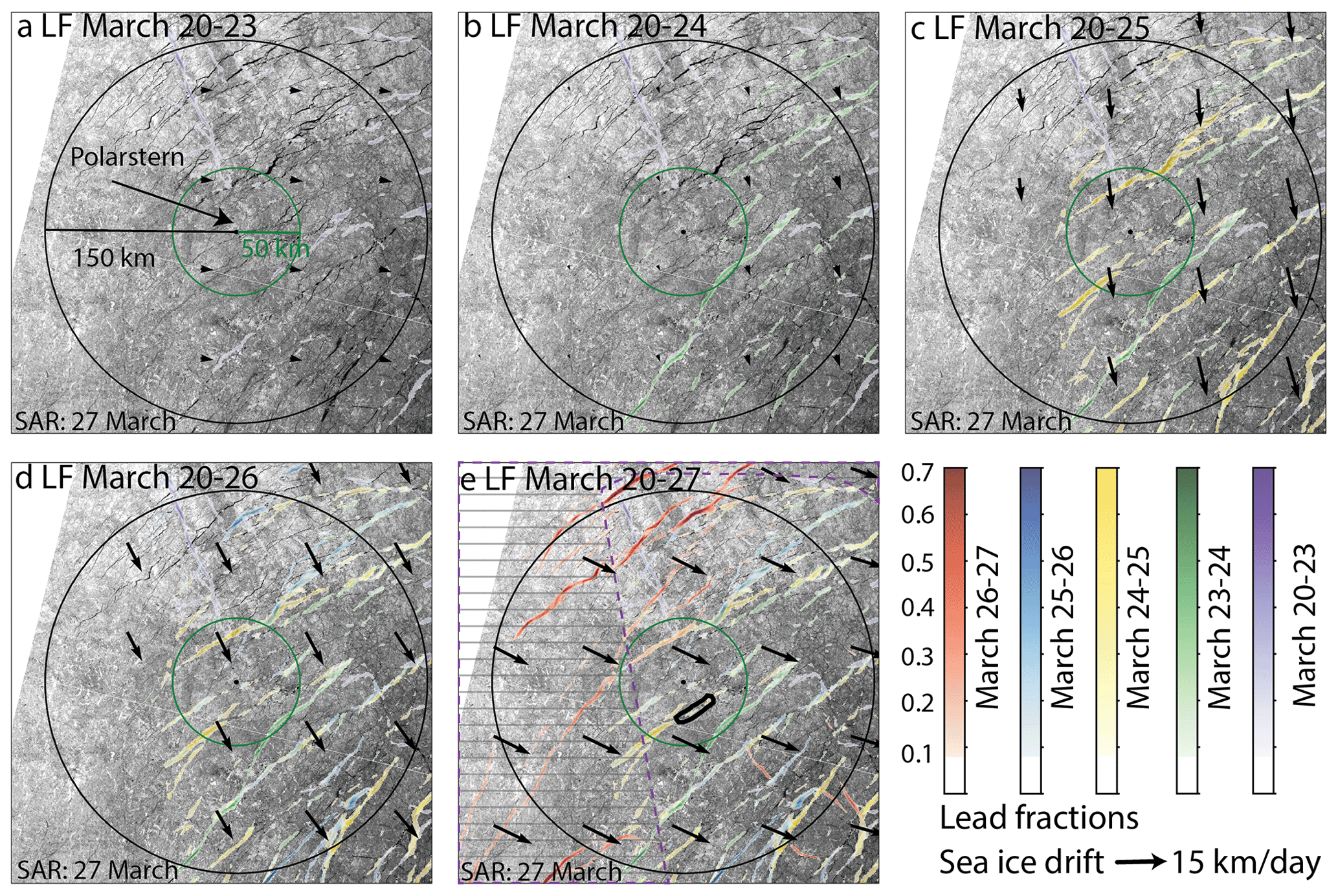
Figure 2Example of accumulated divergence-derived lead fractions (LFaccu. div) from 20 to 27 March. The Sentinel-1 image from 27 March is overlaid by advected lead fractions from different time instances. The colors indicate the timing and magnitude of the lead opening. The black arrows show the sea ice velocity of the latest time instance. The black and green circles around the position of R/V Polarstern have a radius of 150 and 50 km, respectively. The non-dashed area in panel (e) indicates where lead fractions from all 7 d are available. The deformation history of the feature encircled by the thick black line within the green circle is shown in Fig. 3. Source of satellite images: ESA/Copernicus.
3.1.1 Deformation history of a single lead
Figure 3 displays the temporal evolution of a lead between 14 and 27 March at near-daily resolution. Prior to 14 March, the ice pack was closed, but bright lines in the SAR backscatter hint at previous deformation events. The lead experienced opening (16–18 March), closing (18–23 March), and reactivation (25–26 March). Please note that the low temporal coverage prevents us from analyzing any sub-daily deformation due to, e.g., tides. We calculated the width of that lead from the lead fractions assuming that all the divergence resulted in opening in one direction. We evaluated the lead width estimates against visually detected changes in the backscatter of the SAR image. Our estimates slightly underestimate the manually measured widths of 1.8–2.0 and 1.2–1.5 km on 19 and 27 March, respectively. On those 2 days, the presence of frost flowers on the lead ice turned the leads into a highly diffuse scattering surface with a strong backscatter contrast to the surrounding ice. We do not provide manual estimates for the other days as wind-affected new ice formation and finger rafting quickly transformed the smooth lead ice into a rough surface whose SAR backscatter signal was indistinguishable from the surrounding ice.
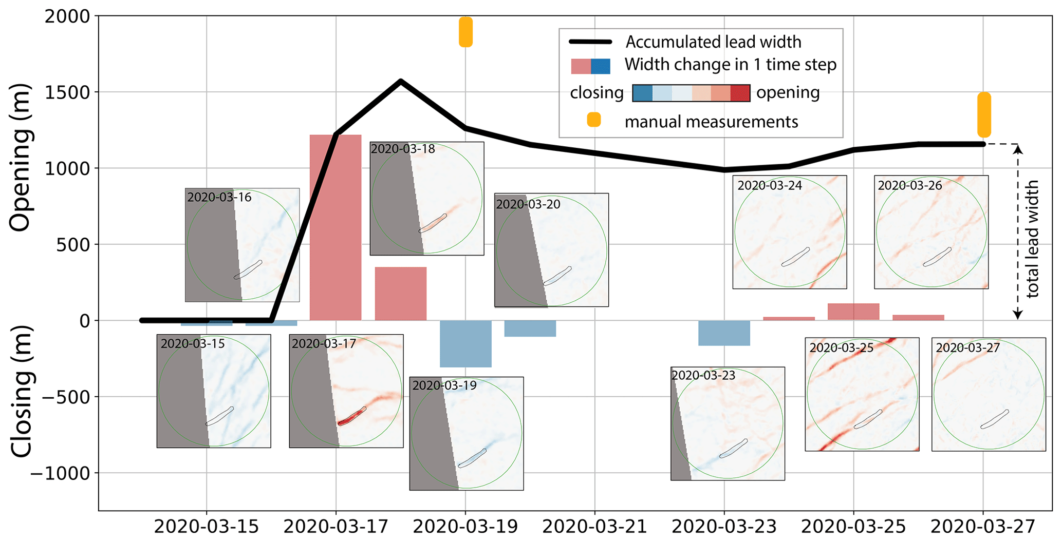
Figure 3Time series of lead opening, closing, and reactivation from 14–27 March. The aerial plots show opening (red) and closing (blue) in a circle with a 50 km radius around R/V Polarstern. The values of the pixels within the dashed line were averaged and are shown by the blue bars. The black line connecting the blue bars accumulates the opening and closing given by the blue bars. The lead width was calculated from the lead fractions assuming that divergence took place only in one direction.
This example provides valuable insights into the life cycle of leads and the capability of the accumulated lead fraction product to resolve the different phases of opening, closing, and reactivation. As expected from modeling studies (e.g., Wilchinsky and Feltham, 2011), divergence and convergence on consecutive days were concentrated on the same ice that was already weakened by previous deformation. We can resolve the thin ice present on March 27 only when accumulating lead fractions over several days, as demonstrated by this example. Combined with a thermodynamic growth model, one could calculate the thickness of the thin ice at any time step (see, e.g., Kwok and Cunningham, 2002; Kwok, 2006).
3.1.2 Statistical analysis of lead lifetime, reactivation, and lead width
The accumulated divergence-derived lead fractions provide valuable information for conducting statistical analyses on various properties of leads, including lead lifetime, reactivation percentage, and lead width. In total, we have analyzed and summarized the properties of 183 562 lead pixels.
Lead lifetime characterizes the duration a certain lead was open within the study period of 10 time instances. Figure 4 displays the time series and distribution of lead lifetimes. The lifetime distribution (p(x)) can be fit by a negative exponential function of the form with an exponent a=0.39 d−1 (Fig. 4b, left y axis). Analyzing the accumulated relative frequency (Fig. 4b, right y axis), we observe that the most common lifetime is 2 d, accounting for 43 % of the leads. This coincides with the shortest lifetime we can resolve; i.e., the actual most frequent lifetime might be shorter. The median lifetime is 3 d, indicating that 50 % of the leads close within this time frame. After 5 d, 83 % of the leads have closed, while only 0.9 % (corresponding to 1652 lead pixels) remain open longer than 10 d. Phases of reduced lifetime often coincidence with strong convergence events (green shading in Fig. 4a), while there is no link for others (orange shading in Fig. 4a). The large standard deviation of each time instance indicates additional spatial variability despite being influenced by similar large-scale wind and ocean forcing.
Reactivation refers to the reopening of a previously closed lead. Over the whole time series, on average 10.7±7.6 % of the leads were reactivated within the 10 time instances. The reactivation percentage can reach up to 36 % at the end of December, as shown in Fig. 4a.
Lead width, as defined in the previous section, is depicted in Fig. 5. The smallest lead width which we can detect must exceed the uncertainty of the lead fraction, i.e., 56–112 m (see Sect. 3.1.3). We have chosen 56 m as the lower limit. As expected, the lead width is a heavy-tailed distribution with lead widths of up to 1300 m. Beyond 1200 m the power-law relationship breaks down, which is why we define 1200 m as the upper detection limit of our algorithm. Nevertheless, leads wider than 1.2 km can still be resolved in our data product by summing up several pixels along the opening direction because their actual width is smeared out over several pixels. Fitting a power-law of the form to the distribution p(w) of the lead widths w after excluding widths w> 1200 m yields an exponent of b=2.55.
In conclusion, the dataset presents a valuable resource for studying the physical and mechanical properties of leads larger than 56–112 m. Combined with ice pack properties, forcing fields, and a thermodynamic growth model, a detailed analysis of the dataset can reveal an in-depth process understanding of sea ice mechanics and their role in the sea ice mass balance.
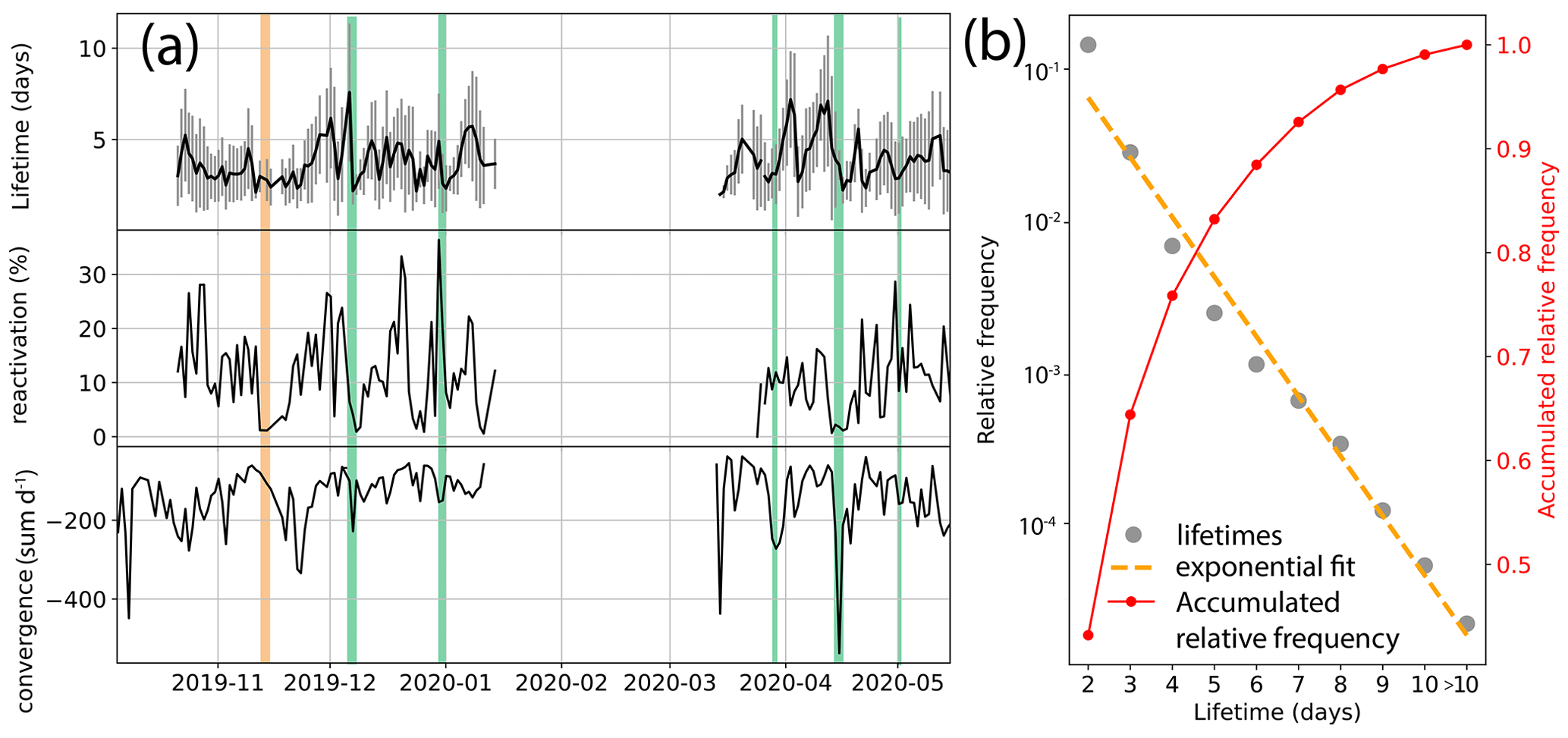
Figure 4Time series (a) and distribution (b) of lead lifetime based on the complete dataset. Panel (a) displays the time series of the mean (± standard deviation) lead lifetime of each day, reactivation percentage, and spatially summed-up convergence. Green shading highlights convergence events with an impact on the lifetime, while orange shading highlights reductions in lifetime without corresponding strong convergence events. Panel (b) shows the distribution of all lead lifetimes (gray, left y axis) and the exponential fit (orange, left y axis). The right y axis shows the accumulated density distribution of the lifetimes.
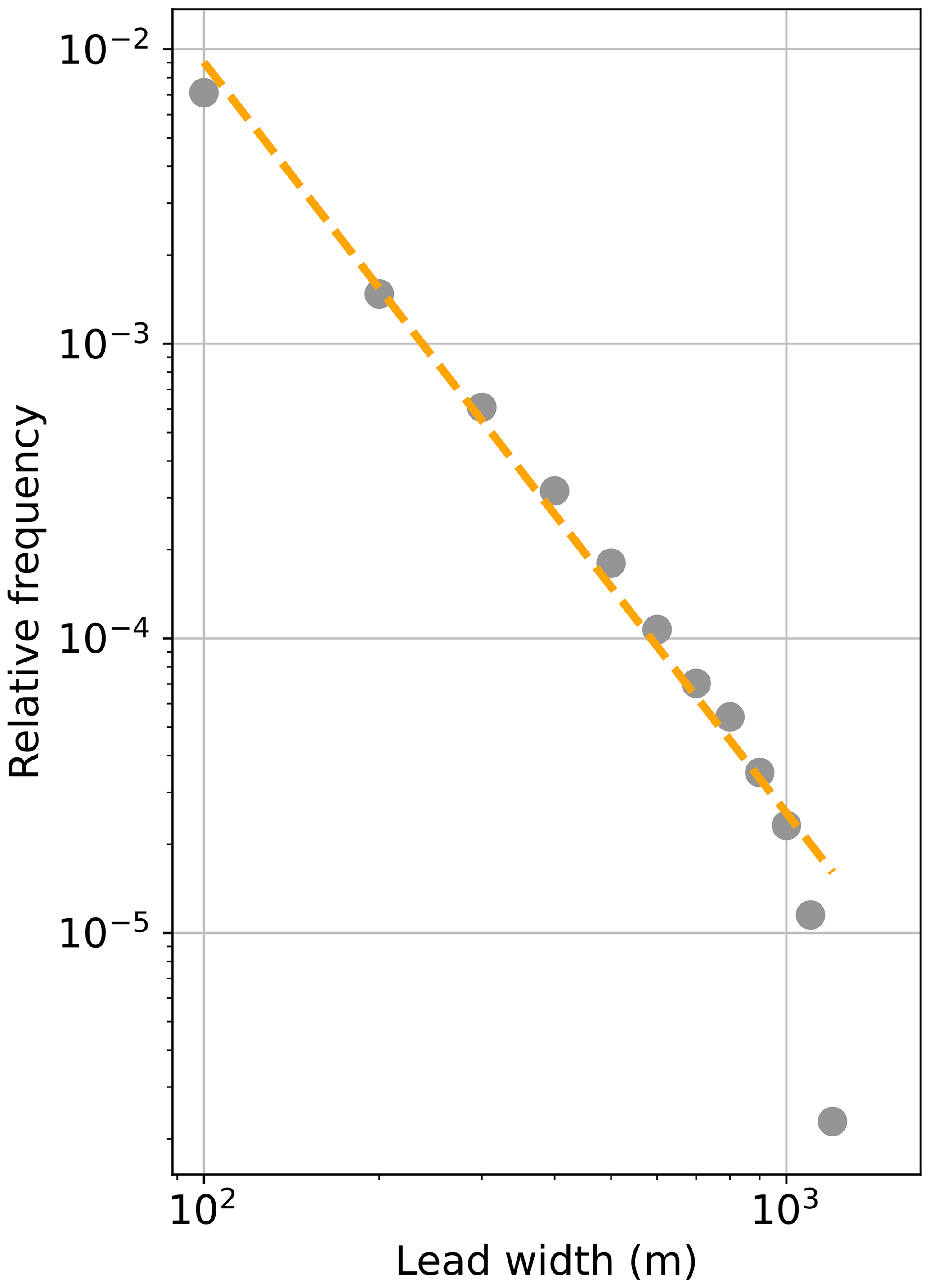
Figure 5Distribution of lead widths based on the complete dataset in a log–log plot. Lead widths are shown as gray dots, and the power-law fit to lead widths ≤1200 m is in orange.
3.1.3 Uncertainties of the accumulated divergence-derived lead fractions
We identify two main sources of uncertainty in the accumulated divergence-derived lead fractions: (1) uncertainty related to the advection scheme and (2) uncertainty of the lead fraction magnitude. In addition, there are lower limits for the lead lifetime and lead width due to the temporal and spatial sampling limitations of the dataset.
The uncertainty of the advection scheme originates from errors in the drift calculations. Hollands and Dierking (2011) state a tracking uncertainty of ±0.8–1.6 pixels, i.e., ±40–80 m. Assuming a homogeneous drift field, the tracking uncertainty accumulates to a maximum of 400–800 m, i.e., one grid cell of the lead fraction product. For a strongly heterogeneous drift field, von Albedyll et al. (2021a) estimated an accumulated tracking uncertainty of 1200 m for 10 time instances using the same drift algorithm (see their Fig. 1 in the Supplement). Thus, the uncertainty of the advection scheme is small and of the order of one to two pixels. In the spatial plots, e.g., Fig. 3, we can confirm the high spatial accuracy. The deformation zone stays concentrated in a narrow zone without any signs of significant “smearing out” due to possible discrepancies in the advection scheme.
To quantify the uncertainty of the lead fraction magnitude, we first simplify the calculation of the dimensionless lead fractions by omitting the time difference information. The lead fractions can also be expressed as the ratio of the difference in displacement (ΔDisp) and the grid cell length scale (L=700 m), thus . Based on the simplified equation, we calculate the uncertainty of the lead fraction magnitude of a single time instance from the tracking uncertainty using error propagation assuming no geolocation errors following Dierking et al. (2020). Adapting their Eq. (17), the uncertainty of the lead fractions σLF is given by the ratio of the tracking uncertainty σtr and the spatial scale given by L:
With a tracking uncertainty of σtr=40–80 m (Hollands and Dierking, 2011) and a grid cell length of L=700 m this results in an absolute error of σLF=0.08–0.16 for one lead fraction pixel. Translated into lead width in a single pixel, this corresponds to 56–112 m when assuming that the lead has opened only along one dimension. For the accumulated lead fractions, we add the absolute errors of each time instance assuming that they are independent. Averaging over larger spatial scales assuming independent errors, we quantify the standard error of the mean accumulated lead fractions using
where k is the number of accumulations and n is the number of pixels that fit into circles with radius 10, 50, 100, and 150 km. For LF, this calculation yields uncertainties for the spatially averaged lead fractions of –0.038 (10 km), –0.008 (50 km), –0.004 (100 km), and –0.003 (150 km).
As uncertainties grow with more accumulation steps, we explore the upper and lower limits of the number of accumulation steps. In winter, thermodynamic growth sets an upper limit on the accumulation time instances. Rapid ice growth can “thermodynamically close” a lead within a time frame ranging from a few hours to days. This duration depends on air temperatures and the maximum ice thickness that still qualifies as a lead. We chose 10 time instances corresponding to at least 10 d as an upper limit. Under the typical (winter) growth conditions during MOSAiC, lead ice thickness reached on average more than 30 cm (min:1 cm, max:50 cm) after 10 d (Nicolaus et al., 2022) which is thicker than what most studies consider to be lead ice. The dynamic lifetime of the leads sets the lower limit of the required accumulation steps. We compared the time series with zero to 10 accumulation steps and found that five accumulation steps can explain roughly three-quarters of the magnitude and variability of the “full” LF time series. This fits well with the observation that 72 % of the leads are closed after 5 d (see Fig. 4b, Sect. 3.1.2). Hence, we suggest using at least five time instances (LF) to describe the temporal evolution of the leads.
3.1.4 Time series of accumulated divergence-derived lead fractions during MOSAiC
The mean (accumulated) LFaccu. div ranges between 0.61 % (LFdiv, no accumulation) and 3.2 % (LF, 10× accumulated) with a maximum of 3.3 % (LFdiv) and 10.3 % (LF), respectively. Figure 6a displays the time series of (accumulated) LFdiv for different numbers of accumulation steps, where LF is highlighted in black. In the following, we will focus on the LF time series.
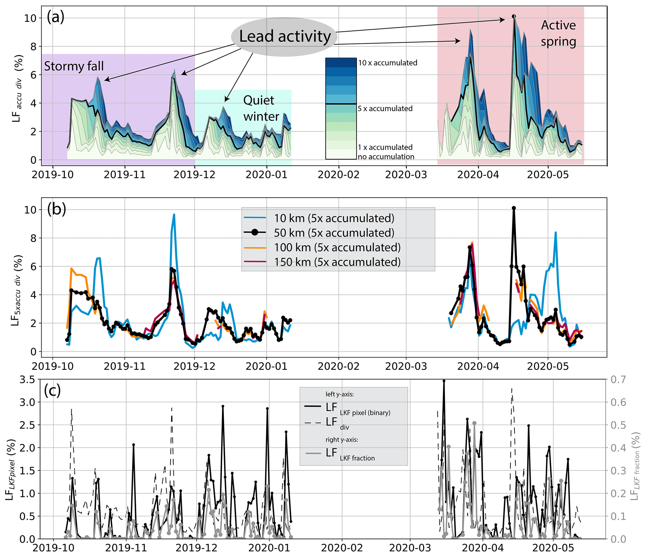
Figure 6LFaccu. div and LFLKF time series. Panel (a) shows accumulated LFaccu. div on the 50 km scale with a varying number of accumulation time instances. The time series with LF is highlighted in black. The three main phases and several periods of higher lead activity are marked with colored shading and arrows, respectively. Panel (b) compares LF of different spatial scales. Panel (c) shows on a 50 km spatial scale the binary lead pixel number LFLKF pixel and LFdiv on the left y axis and LFLKF fraction lead fractions on the right y axis (mind the different scales).
The LF time series is roughly split into three phases: a stormy fall (October–November), a quiet winter (December–January), and an active spring (March–May, Fig. 6a). Those phases align with the general seasonality of the dynamic regime during the MOSAiC drift (Angela Bliss and Jennifer Hutchings, personal communication, 2022, see also, e.g., Krumpen et al., 2021; von Albedyll et al., 2022, for sea ice dynamics along the drift). Within the three main phases, there are several peaks of lead activity lasting 1–1.5 weeks (arrows in Fig. 6a). The highest lead activity, characterized by multiple events of a duration of 1–2 d with high lead fractions, was reached in March 2020, when R/V Polarstern was in the western Nansen Basin, a region that is generally characterized by high lead fractions (Fig. 15 in Krumpen et al., 2021). Interestingly, the frequency of lead events stayed roughly constant during the seasons, but their larger magnitude and persistence in fall and spring created the offset in the accumulated lead fractions. When interpreting this time series, one needs to keep in mind that thermodynamic growth quickly covers leads with new ice.
The three phases correspond well to the atmospheric forcing and the consolidation state of the ice pack. In the fall when R/V Polarstern was located in the Siberian Arctic, the sea ice was still freezing up and was hit by an elevated number of cyclones in November (Rinke et al., 2021; Nicolaus et al., 2022; von Albedyll et al., 2022). In the quiet winter phase in the central Arctic (here only documented until the middle of January), the ice pack consolidated completely with only one cyclone passing through in December. In the active spring, cyclone activity increased again and a sequence of storms first broke and then easily deformed the ice pack (Rinke et al., 2021; Nicolaus et al., 2022). This increase in lead activity corresponds well to R/V Polarstern approaching the western Nansen Basin, a region that is generally characterized by higher lead fractions (Fig. 15 in Krumpen et al., 2021).
3.1.5 Accumulated divergence-derived lead fractions on different spatial scales during MOSAiC
Figure 6b compares LFaccu. div of different spatial scales, described by circles with radii from 10 to 150 km centered around R/V Polarstern. Lead fractions of the different scales are generally similar in magnitude and temporal evolution. They differ less than the different accumulation time instances. This means that the deformation was more consistent on spatial scales up to 150 km than persistent on temporal scales >5 d. However, on the smallest spatial scale of 10 km, we note some clear deviations from the overall pattern. On the smaller scale, the localized and intermittent nature of deformation (e.g., Marsan et al., 2004; Hutchings et al., 2011) starts to become apparent with localized lead events hitting (or missing) the smaller area. Due to the lower data coverage, the time series of 100 and 150 km are incomplete as we only consider points with coverage >50 %. We conclude that the 50 km time series is representative of the larger surroundings of the MOSAiC central observatory based on a high correlation of >0.9 with the 100 and 150 km time series.
3.2 LKF-derived lead fractions
Figure 6c presents the LKF-derived lead fractions. The binary lead pixel number LFLKF pixel is displayed together with the native product LFdiv on the left y axis, and the LKF lead fractions LFLKF fraction are shown on the right y axis (different scale). LFLKF pixel has a similar magnitude as the LFdiv with a mean of 0.65 % and a maximum of 3.46 % (on 15 March 2020). In contrast and as expected from the processing, the average of the LFLKF fraction is 2 orders of magnitude smaller than LFdiv with a mean of 0.05 % and a maximum of 0.51 % (on 28 March 2020). Both time series exhibit a very similar temporal variability, which is why we summarize them together as LFLKF. Because LFdiv and the LFLKF are based on the same divergence fields, the observed very similar temporal variability (Pearson R=0.78) is expected. In contrast to the LFdiv time series, lead events in the LFLKF time series are more prominent, clear signals in the time series with otherwise mostly zero values.
The observed differences align well with the differences in the retrieval techniques. The LKF detection algorithm of the LFLKF functions as a strict filter on LFdiv by reducing unwanted noise and highlighting strong events. However, it also removes most likely real divergence events that are either not strong enough or do not result in elongated shapes. The agreement between the magnitudes obtained from LFLKF pixel and LFdiv results in several conclusions. By assigning a lead fraction of 1 to every LKF pixel, we end up overestimating the lead fraction. This happens because only 0.4 % of all lead pixels contain leads wider than 700 m (as depicted in Fig. 5). Yet, this overestimation is counteracted by the morphological thinning of leads into 1-D features. Both effects seem to compensate for each other on average. Therefore, we conclude that LFLKF pixel is a first guess to concentrate the spread-out lead signal in the divergence data into a single pixel. It is important to note that, unlike LFaccu. div, LFLKF only considers newly formed leads.
This section compares the results of our two new lead products with results from the six existing lead products described in Sect. 2.3. We compare the time series with respect to their mean values (Sect. 4.1), their temporal variability (Sect. 4.2), their temporal and spatial coverage (Sect. 4.3), and their ability to resolve leads spatially (Sect. 4.4).
We restricted our analysis to the time period from 5 October 2019 to 15 May 2020. During the subsequent melt season, most of the retrieval methods suffer from large uncertainties and are thus not available. For the temporal comparison, we compared mean lead fractions in a circle with a 50 km radius around the position of R/V Polarstern at the acquisition time of the SAR images. We chose this scale because it is representative of the wider surroundings (see Sect. 3.1.5), captures the LKF structures, comprises the extended network of measurements conducted during MOSAiC, and is a compromise between the different resolutions and coverage of the various lead products. For the timescale of the accumulated lead fractions, we have chosen LF (see Sect. 3.1.3).
4.1 Mean and variability of different lead products
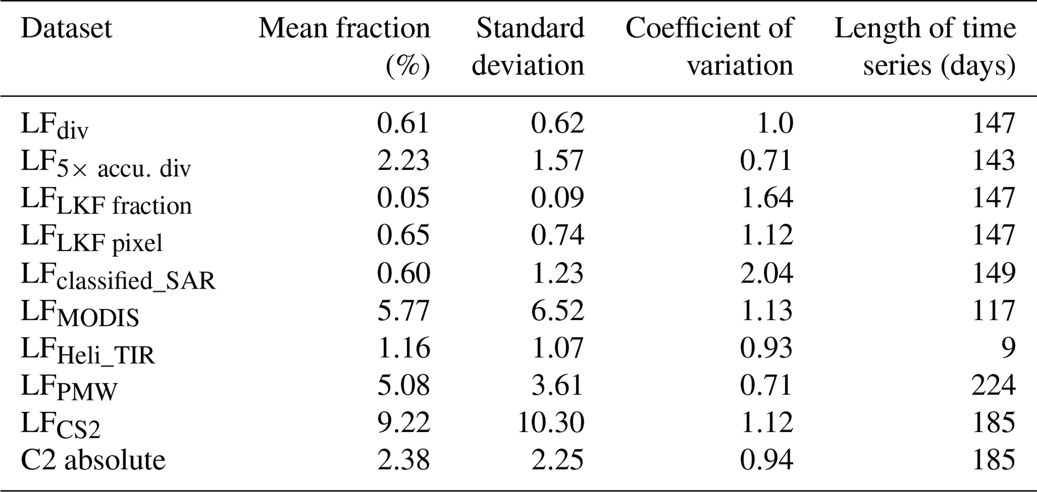
Table 1 provides a summary of the average lead fractions from various time series along with their respective variability measures, represented by the standard deviation and the coefficient of variability. The coefficient of variability is calculated as the ratio of the standard deviation to the mean value, serving as an indicator of the relative variability for each set of data.
The mean lead fractions among the lead products vary by 2 orders of magnitude between 0.05 (LFLKF fraction) and 9.22 % (LFCS2), while their variability is very similar with coefficients of variability between 0.71 and 2.04. For a plausibility check of the magnitude of the lead fractions, we compare the mean lead fractions to mean open-water fractions derived from airborne ice thickness observations during MOSAiC reported in von Albedyll et al. (2022), which describes the abundance of open water and 1–10 cm thick ice. Thus, this dataset approximates the fraction of leads that opened up on that particular day or slightly before in the freezing season. Taking the average of all nine surveys between October 2019 and April 2020 gives an open-water fraction between 0.02 % and 0.81 % with a mean of 0.35 %. This number most likely underestimates the true open-water fraction due to the footprint averaging of the EM airborne ice thickness measurements. Nevertheless, it provides a rough estimate in the same order as the mean LFdiv, LFclassified_SAR, and LFHeli_TIR.
The observed differences in magnitude provide clear evidence for the major differences in the “lead definition” (Sect. 2.1) of each retrieval method, but also in their spatial and temporal coverage and resolution. Since the variability is similar, we suggest that all retrieval methods react similarly sensitively to changes in the real lead fractions, but with different magnitudes. LF, LFMODIS, and LFPMW overestimate the open-water fractions compared to the EM thickness observations. This fits well with the assumption that their lead fractions also include thin ice. However, the LFHeli_TIR is based on the same measurement principle as LFMODIS but has substantially smaller values. Therefore, other factors such as spatial resolution, spatial coverage, and atmospheric conditions also play a role. LFdiv and LFclassified_SAR primarily detect open-water leads, which is supported by their reasonably good fit to the observed EM open-water fractions.
Table 1Average properties of different lead products in a 50 km circle around R/V Polarstern. The mean lead fraction and its standard deviation are given with the coefficients of variation defined as the ratio of the two former quantities. Where available, the mean is given with its uncertainty. C2 absolute is given in absolute numbers, not percentages. The length of the time series varied due to the lack of satellite coverage or data gaps, e.g., due to clouds.
4.2 Temporal variability of different lead products
The seasonal variability of the LFclassified_SAR time series is similar to the one of the LFdiv and the LFLKF with more active phases in fall and spring (Fig. 7, note the different y axes). The time series of LFclassified_SAR has several active phases or individual events in common with the divergence-based products, which are marked in red in Fig. 7 and labeled a1–a6. For the first very active phase in October (a1) there is no one-to-one correspondence between the individual lead events, but all available datasets, including the LFCS2, indicate the presence of several leads. Between November and March (a2–a6), the LFclassified_SAR agrees with the most pronounced lead opening events in LFdiv and LFLKF that also correspond in most cases to maxima in the accumulated LF. Smaller events that appear exclusively in LFdiv and LFLKF were not consistently identified by LFclassified_SAR. This suggests that the divergence-based products are more adept at capturing lead events than LFclassified_SAR, although they may also contain some noise.
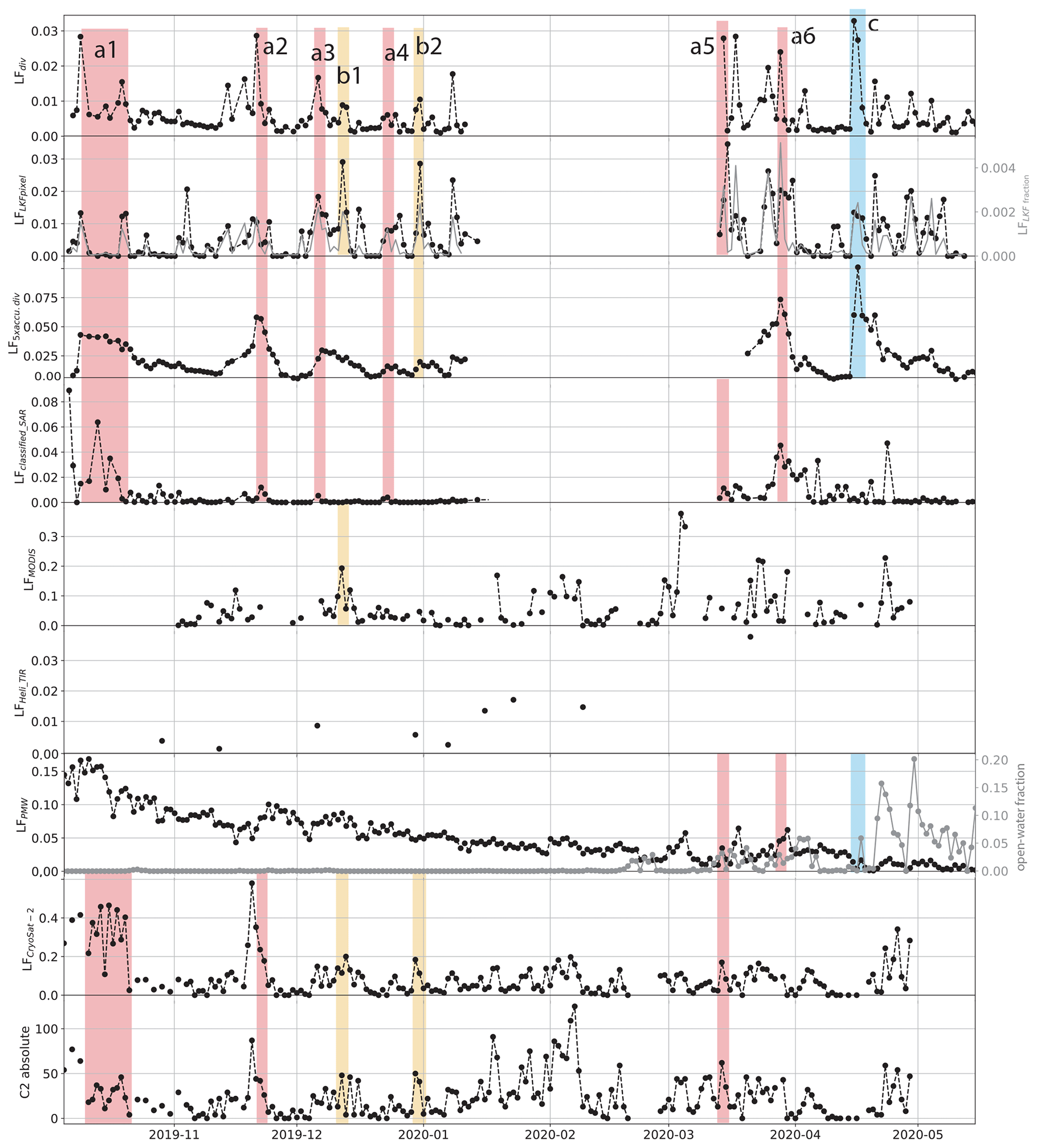
Figure 7Time series of lead fractions from different products. Colored and labeled (a–c) bars indicate common events. Red shading (a1–a6) highlights lead events in the divergence-based products and most other sensors. The yellow shading (b1–b2) shows events visible in the LFCS2, LFdiv, and LFLKF time series. The blue shading (c) highlights the strongest lead event in the LFdiv and LFaccu. div. The scale of the different y axes varies substantially. LFLKF fraction is plotted on the right y axis together with LFLKF pixel (second panel). Open-water fraction, calculated as 1 − ice concentration, is plotted on the right y axis together with LFPMW (seventh panel).
There are also pronounced differences between LFclassified_SAR and the divergence-based lead fractions. For example on 15–16 April 2020, the strongest lead event of LFdiv (blue shading, c) lacks a counterpart in the LFclassified_SAR. In fact, this peak corresponds to a large shear zone in the study area, creating open water and ice rubble.
It is interesting to note that the duration of the individual events in the LFclassified_SAR times series is typically 1–2 d, similar to LFdiv and LFLKF, while the lower-frequency variability of LFaccu. div indicates that some of the leads stayed open longer than a day. We thus conclude that LFclassified_SAR predominantly detects open water and only to a minor degree leads covered by thin ice.
Frequent data gaps in the LFMODIS time series due to clouds complicate a comprehensive comparison. The seasonal evolution agrees with the ones of the other time series with high lead fractions in March 2020. One major event in December 2019 (yellow shading, b1) is shared with LFdiv, LFLKF, and LFCS2 but has a much larger amplitude in LFMODIS.
The LFHeli_TIR time series consists only of nine temporal snapshots, which prevents an in-depth interpretation of the variability. In addition, the helicopter-borne dataset is very limited in space. Overall, the trend, suggested by the few data points, towards higher fractions in spring, aligns well with the other lead fraction time series.
The LFPMW time series shows a gradual decline in lead fraction from fall to spring, a trend not observed in the other time series. Notably, for the first time, zero lead fractions are recorded around mid-March, coinciding with a shift in the general pattern, leading to the emergence of more distinct events. Among these events, three coincide with events observed in other products (a5–a6). It is important to mention that during the strong shearing event on 15–16 April 2020, the ice concentration (shown as the open-water fraction, 1 − ice concentration, on the right y axis in Fig. 7) decreased, while the lead fraction remained small. Based on our observations, we propose that the gradual decrease in LFPMW primarily reflects the thermodynamic thickening of thin ice rather than a change in the presence of leads. However, starting from mid-March, LFPMW appears to predominantly capture thin ice formed in refrozen leads while being less sensitive to open water, as evidenced by the 15–16 April event. Please note that the strong decrease in concentration after 16 April is related to the effect of glazing on the retrieval algorithms due to a warm-air intrusion (Rückert et al., 2023).
The seasonality of the LFCS2 time series is slightly different from the divergence-based lead products, with the highest lead activity in fall and only a few events recorded in spring. With this, it corresponds better to LFclassified_SAR. Potential causes of this deviation could arise from the abundant thin ice in the fall that could have been classified as leads by the retrieval algorithm. Similar to LFLKF, the LFCS2 time series consists of events that normally last 1–3 d and can be easily separated from each other. There is good agreement between the LFCS2 and several other products for several events (a1, a2, a5). In addition, they agree with LFdiv and LFLKF on additional events in December 2019 (yellow shading, b1–b2). The LFCS2 suffers from a low spatial coverage that likely causes a sampling bias in the lead indication. For example, the ice affected by the major lead event in the middle of April (blue shading, c) was not covered by the swath of the satellite.
Overall, for periods shorter than the seasonal cycle, there is only anecdotal agreement between the different lead product time series. This lack of general similarity strongly complicates establishing some kind of “common ground” for the evaluation of lead products.
4.3 Temporal and spatial coverage of different lead products
Lastly, we compare the temporal resolution and coverage of the different lead fraction products along the MOSAiC drift. Table 1 shows that LFPMW is the most complete time series, while LFMODIS has the fewest valid days. The divergence-based time series perform in the midfield; however, they suffer from a very irregular distribution of the gaps caused by the lack of satellite coverage north of approximately 87° N. Especially in those regions, lead fractions from sensors other than Sentinel-1 and most other SAR satellites are crucial. While those results are specific for the MOSAiC drift track, they still demonstrate the limiting factors of the different time series that are either sensor-specific (no coverage beyond a certain latitude) or due to the retrieval technique (clouds).
4.4 Spatial comparison of different lead products
The previous sections were concerned with comparing mean values and temporal variability. Next, we analyze how well LFdiv, LF, and LFLKF reproduce the location and size of the same leads compared to a visual reference. To do so, we focus on two case studies in November 2019 and March 2020 with different dynamic regimes.
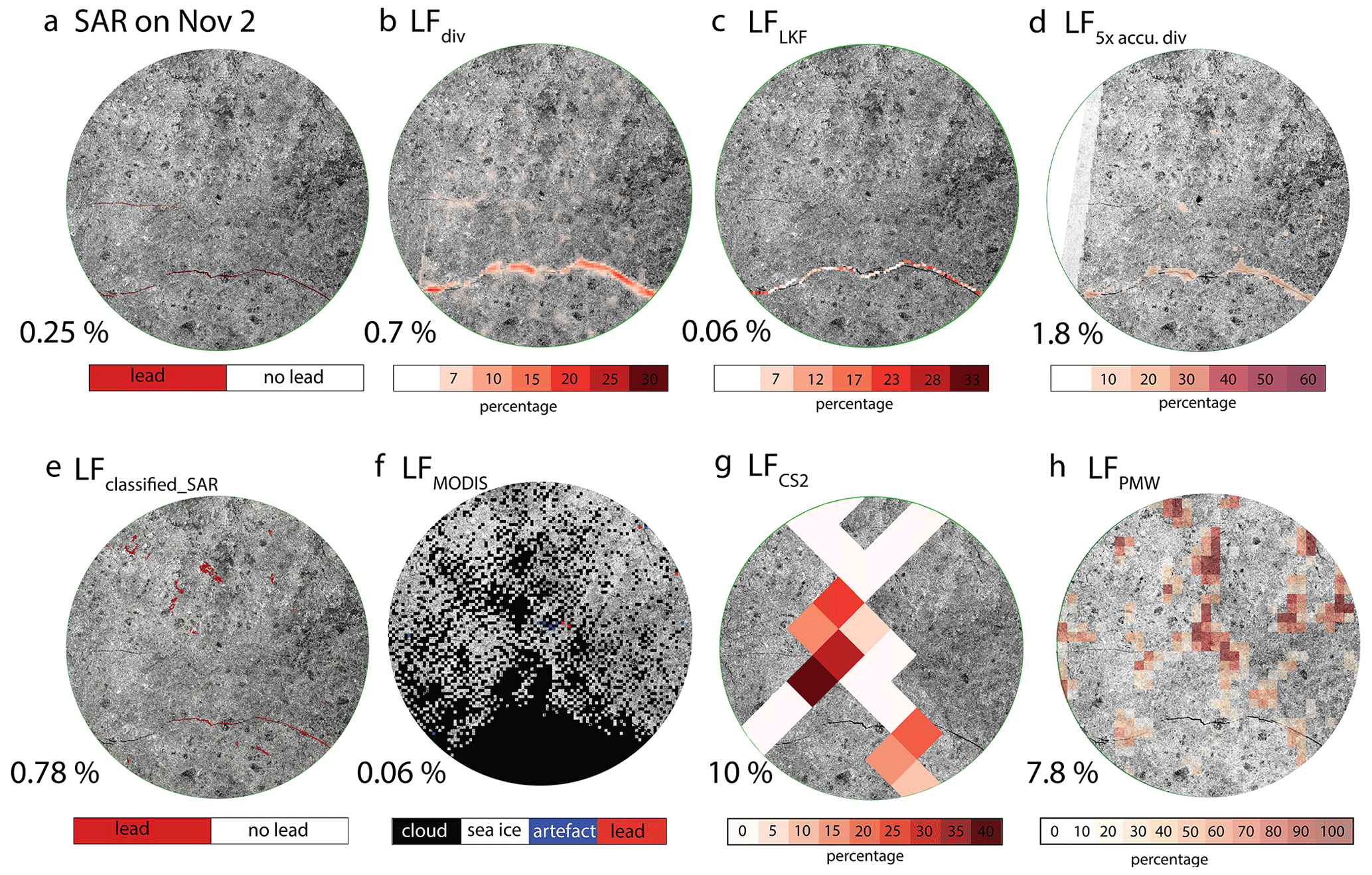
Figure 8Comparison of different lead products on 2 November 2019. Panel (a) displays a SAR image of the ice pack on 2 November 2019, with two leads identified manually. Panel (b) displays the advected LFdiv. Panel (c) shows the advected LFLKF fraction. Panel (d) shows the advected 5× accumulated LF. All other lead products are shown in the second row. The LFMODIS values in panel (f) are strongly affected by clouds (black). The few lead pixels (red) are located close to the center of the circle. The numbers at the bottom left of each panel indicate the lead fraction. All circles have a radius of 50 km and are centered on the position of R/V Polarstern. Source of satellite images: ESA/Copernicus.
4.4.1 Single deformation event – 1–2 November 2019
Between 1 and 2 November 2019, two leads opened in the previously closed ice pack (Fig. 8b). An approximately 70 km long and 350 m wide lead opened 25 km south of R/V Polarstern (manually measured on the SAR image with 50 m resolution). A smaller lead with 33 km length and a maximum width of 250 m opened 11 km to the west of the ship (manually measured on the SAR image with 50 m resolution). Both leads were closed again on 3 November 2019. Extrapolating from the ice thickness observations from 14 October to 1 November 2019, the modal ice thickness of the surrounding ice was likely around 0.5 m±0.1 m (von Albedyll et al., 2022).
We manually estimated a lead fraction of 0.25 % from the SAR image (Fig. 8a). The LFdiv captured the larger lead very well. As the only lead product, the LFdiv partly also indicated the formation of the smaller lead. We tested whether the observed width of the lead and the integrated divergence values along the opening direction of the lead match. We found that the LFdiv results in a lead width of 300–350 m, which agrees well with the observed 350 m. However, the LFdiv also indicates divergences at several other spots where we could not find any visual signs of open water. This results in a slight overestimation of the lead fraction (0.7 %). Those spurious detections are removed in the LFLKF fraction but at the expense of also removing any sign of the smaller lead. Since the larger lead is concentrated into a quasi-one-dimensional structure that is only one pixel wide, the estimate of the lead width is reduced to about 200–240 m. Altogether, this results in only a small lead fraction of 0.06 %. The accumulated lead fractions LF show a similar distribution to LFdiv, as anticipated due to the closed ice pack on 1 November 2019. The accumulation of false detections results in a higher lead fraction of 1.8 %.
The LFdiv, LFLKF fraction, and LF perform similarly well as the LFclassified_SAR in detecting the location of leads. The LFclassified_SAR benefits from a high spatial resolution that is 1 order of magnitude larger than the one of LFdiv and LFLKF and captures the large lead precisely. However, the lead classification algorithm used reliably detects only leads with a minimum width of about 200 m, corresponding to five pixels of the original Sentinel-1 SAR scenes. More narrow leads and parts of a larger lead are not always classified as open water. The LFclassified_SAR detects additional features that are not visually identified as leads, similar to LFdiv. This leads to an overestimation of the lead fraction by 0.78 % compared to the visual estimate. While LFMODIS suffers from heavy cloud coverage (lead fraction: 0.06 %), the LFPMW (7.8 %) shows some features that are most likely associated with thin ice rather than leads. CryoSat-2 passed over the small lead and parts of the larger lead and captured higher lead fractions. The higher LFCS2 of 10 % confirmed the overall divergent drift regime that has probably opened a few additional smaller leads that are not visible on the SAR image.
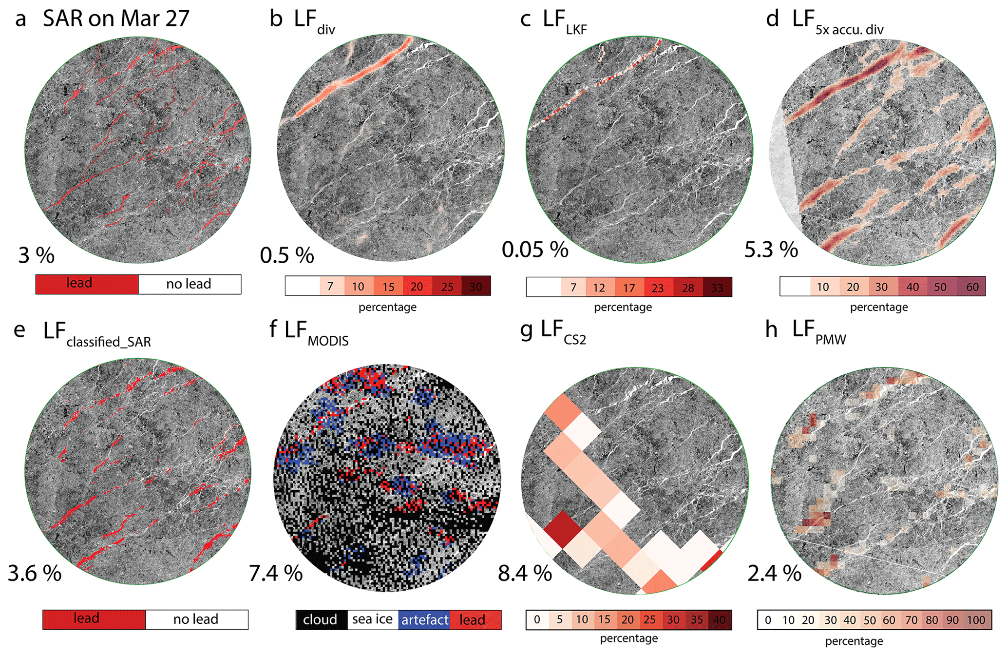
Figure 9Comparison of lead products on 27 March 2020. Panel (a) displays a SAR image of the ice pack on 27 March 2020, with the largest leads identified manually. Panel (b) displays the advected LFdiv. Panel (c) shows the advected LFLKF fraction. Panel (d) shows the advected 5× accumulated LF. All other lead products are shown in the second row. The numbers at the bottom left of each panel indicate the lead fraction. All circles have a radius of 50 km and are centered on the position of R/V Polarstern. Source of satellite images: ESA/Copernicus.
4.4.2 Dynamic phase with several leads opening – 26–27 March 2020
The period of 26–28 March 2020 was very dynamic with lead openings and closings. Several leads up to 1 km wide opened within 50 km distance to R/V Polarstern. Due to the low temperatures around −30 °C, the open water quickly refroze (Nicolaus et al., 2022; Shupe et al., 2022). The modal and mean ice thickness was around 1.7 and 2.3 m, respectively (von Albedyll et al., 2022).
We manually estimated a lead fraction of 3 % concentrating on the large lead systems (Fig. 9a). Leaving out a few smaller leads, this value probably still underestimates the true lead fraction. The LFdiv reproduces the opening of the leads in the upper left part of the 50 km circle (Fig. 9b). The respective divergence fields show that there was weak convergence along most of the other lead locations. The fraction of 0.5 % only reflects the newly formed leads. LF shows that most of the leads in the lower part of the circle had formed during the previous time instances (see also Fig. 2) and suggests a higher lead fraction of 5.3 %. The visual estimate of 3 % falls between the two products. This makes sense when considering the rapid formation of new ice in the leads that are several days old with the associated change in radar backscatter. For this case, the LF with 3.3 % comes closest to the visual estimate.
Like LFdiv, the LFLKF fraction only indicates the active deformation zone in the upper left part of the study region and a lead fraction of 0.053 %. Analog to the LFdiv, the LFLKF fraction showed a high fraction of 0.15 % the day before on 26 March 2020. The LFLKF fraction further filtered out the weak convergence signals visible in the divergence lead fractions.
The LFclassified_SAR comes closest to the manual estimate in magnitude (3.6 %) and in location thanks to its high spatial resolution. In contrast to LF, LFclassified_SAR does not identify some of the older leads, which is in line with the general assumption that LFclassified_SAR best resolves leads with open water and smooth, thin ice. With a fraction of 2.4 %, the LFPMW is still close to the visual estimate, but the analysis of the spatial distribution showed that the LFPMW product only resolves parts of the leads (Fig. 9h). Nevertheless, in contrast to the November case, the LFPMW significantly improved in predicting the location of leads for the March case, as the few resolved structures were clearly aligned with leads seen on the SAR image (Fig. 9h). When not cloud-covered, LFMODIS detected individual leads, but not reliably. Interestingly, the LFMODIS of 7.4 % is still double the visual estimate. We speculate that there are two main reasons for this large estimate. First, where leads are correctly identified, the fraction is overestimated due to the combination of gridding and the binary classification scheme (see Sect. 2.3.2). Second, MODIS is detecting leads in some areas where leads were not observed visually, especially between detected leads. This could hint at the presence of thinner leads that are not seen on the SAR image, warmer air around a lead that “smears out” the lead signal, or old leads with thicker ice that is not seen by the other retrievals. The LFCS2 indicates a lead fraction of 8.4 %, which is lower than for 2 November 2019, despite more leads being present. Even though the swaths indicate some coverage of the leads, the valid waveforms for the lead pixels are rather low. We speculate that the very small leads might have been missed since the corresponding waveforms are also influenced by surrounding sea ice and are subsequently classified as mixed surface type and intentionally removed from the processing. The sufficient lead area fraction within the radar footprint needed for a lead waveform classification is not known and likely depends on the actual geometry and specific lead radar backscatter characteristics. Lead waveform classification, however, is possible in the presence of sea ice; thus, it is reasonable to assume that the rate of lead detections of radar altimeter data still overestimates the true lead area fraction.
We conclude that a spatial analysis of lead products, e.g., a visual comparison with higher-resolution optical or SAR data and a plausibility check of the shape and stability of detected leads, provides relevant information about the ability of products to indicate leads at the chosen temporal and spatial resolution. The SAR-based lead fractions (LFdiv, LFLKF fraction, LF, LFclassified_SAR) perform best in locating the leads, while the other sensors suffer from low coverage due to clouds or no overpasses, low spatial resolution, the presence of thin surrounding ice, or leads that are too small.
The objective of this study was to analyze lead products based on divergence. We have calculated two lead products from the divergence: divergence-derived (accumulated) lead fractions (LFdiv) and LKF-derived lead fractions (LFLKF). In the subsequent sections, we will first examine the uncertainties (Sect. 5.1), as well as the advantages and disadvantages, of the LFdiv and LFLKF methods in comparison to other lead datasets (see Sect. 5.2). Following this, we will compare our lead statistics with those reported in other studies (Sect. 5.3). Finally, we will discuss potential applications of lead fractions based on divergence (Sect. 5.4).
5.1 Uncertainties of the lead fraction products
In Sect. 3.1.3, we assessed the standard error for the spatial mean (50 km) of LF, ranging from to 0.008. For the whole time series (Table 1), this results in an absolute error between 0.33 % and 0.66 % in lead fractions and, relative to the average lead fraction of 2.23 %, in a relative error of 15 % to 30 %.
Here, we address other uncertainties not yet accounted for. Firstly, the accuracy of divergence-derived lead fractions most likely varies with the deformation rates. On the one hand, given a constant tracking error, the signal-to-noise ratio is larger for larger deformation rates; i.e., larger lead fractions are more certain (Bouchat and Tremblay, 2020). On the other hand, new deformation zones can locally increase the tracking error due to changes in backscatter patterns, complicating the ice displacement retrieval (Griebel and Dierking, 2017). In addition, averaging sea ice velocity over larger scales to remove outliers can reduce the error over areas with homogenous ice drift but obscure deformation lines. Furthermore, the grid’s orientation relative to deformation zones also affects the accuracy of deformation estimates (Bouillon and Rampal, 2015; Griebel and Dierking, 2018). Secondly, our methods miss many small, short-lived leads (<56 m and <2 d, Thielke et al., 2024). Also, we do not capture the life span and width of leads that remain open for over 10 d. Including all leads would alter the mean properties over time. We conclude that divergence-based lead fractions accurately capture when and where a lead opens and closes, but measuring the actual width of leads is less certain.
Comparing the uncertainties of different lead products is complex. The probability of false lead detections in the binary lead products LFMODIS and LFclassified_SAR ranges between 10 %–15 % and 0.8 %–10 %, respectively (Sect. 2.3.2 and 2.3.1). No uncertainty estimates are available for LFCS2 and LFPMW. In addition, the pixel-based uncertainty assessments do not account for biases in temporal–spatial averages in sparsely sampled areas due to limited coverage, swatch width, or clouds. Our comparison forms a basis for improving and reassessing the uncertainty estimates of all products, after accounting for the different lead definitions detailed in Sect. 2. A comprehensive, high-resolution “ground truth” dataset, possibly based on high-resolution thermal infrared data (Qiu et al., 2023) or extensive ICESat-2 lead retrievals (Duncan and Farrell, 2022; Farrell et al., 2020), could further enhance our understanding of these uncertainties.
5.2 Advantages and disadvantages of lead fractions based on divergence
5.2.1 Advantages of lead fractions based on divergence
The first and most important advantage of the LFaccu. div is that combined with the drift information, it resolves the temporal evolution of individual leads. Knowledge of the deformation history of a lead enriches our understanding of the large-scale ice strength and preferred means of sea ice redistribution. When combined with a thermodynamic growth model, it also allows reconstructing the thin ice part of the ice thickness distribution (e.g., Kwok and Cunningham, 2002). Statistics about lead lifetime, reactivation, and total lead width highlight the temporal and spatial variability of the deformation history of leads. Exploring this variability allows us to study changes in the mechanical properties related to ice pack properties across different regions and times and to compare them with sea ice models (e.g., Hutter et al., 2022; Ringeisen et al., 2023).
The second advantage of LFaccu. div is the ability to detect small leads and those that have SAR backscatter coefficients similar to ridges, e.g., caused by ice rubble or frost flower, while maintaining a large spatial coverage. Even though LFclassified_SAR indicates the location of leads with a 10 times higher spatial resolution, LFdiv was most reliable in resolving small leads (<250 m) for the case study from 2 November 2019 (Sect. 4.4). Especially during predominantly shearing motion, when loose ice rubble is created, which still allows for ocean–atmosphere exchange, the LFaccu. div has a clear advantage over the LFclassified_SAR. While LFCS2 most likely includes even smaller leads, LFdiv has the advantage of a higher spatial resolution and larger spatial coverage than the gridded LFCS2.
Third, LFdiv is easy to interpret as the magnitude is directly linked to the formation process of leads. The average magnitude of the LFdiv seems to be a realistic estimate of the open-water fraction compared to complementary high-resolution airborne EM observations. The mean LFaccu. div is larger because is also includes leads covered by thin ice in addition to open water. Combining the deformation history of LFaccu. div with a thermodynamic growth model would enable full control over the maximum allowed thickness in leads. In contrast, the larger LFMODIS and LFPMW classify thin ice up to a certain unknown ice thickness as leads.
Last, all of the time series based on SAR data (LFdiv, LFLKF, LFclassified_SAR) have a high spatial resolution at moderate temporal coverage. The LFLKF indicates the location of the leads with similar precision as the LFclassified_SAR. While LFPMW and LFCS2 provide better temporal coverage than the SAR-based products (Table 1), LFPMW falls short in spatial resolution, and LFCS2 does not match the SAR images in coverage. Surprisingly, in our study, LFMODIS falls behind the SAR time series concerning the temporal coverage due to high cloud coverage. However, LFMODIS has the advantage of covering the whole cloud-free Arctic sub-daily without any gaps north of approximately 87° N. Thus, LFMODIS is better suited for long-term (months to years), pan-Arctic studies of lead fraction trends.
5.2.2 Disadvantages of lead fractions based on divergence
First, the ability of LFdiv to detect small leads comes at the expense of a higher noise level. Therefore, most of the other products use a shape criterion to remove noise. How this could be successfully done on LFdiv is essentially shown in the LFLKF that does not contain any noise but also misses smaller leads. This trade-off between the size of leads and the confidence in them could be adjusted depending on the research question by revisiting the filter of the LKF detection algorithm.
Second, leveraging the full potential of the LFLKF as a noise-free, feature-based lead product requires a more sophisticated approach to derive areal lead fractions. Among the two current methods, LFLKF pixel estimates aligned more accurately with reference data from LFHeli_TIR and EM ice thickness observations. However, a future approach for the extraction of divergence should allow LKFs to have a width of several pixels.
Third, the temporal and spatial coverage of LFdiv and LFLKF is limited. Potentially, this could be overcome by adapting the presented methods to data from other SAR satellites, e.g., the RADARSAT Constellation Mission (Howell et al., 2022), to yield more complete coverage of the Arctic. However, so far, LFPMW and LFMODIS have provided more suitable alternatives for climatological studies reaching back several decades or studies on Arctic-wide scales and (sub-)daily timescales.
5.2.3 Summary
Taken together, based on our means of comparison, we conclude that LFdiv and LFLKF combine advantages of several other lead products and are thus a valuable addition to the existing lead products. This corroborates earlier results from Kwok (2002), Kwok and Cunningham (2002), and Kwok (2006), who used RGPS-derived deformation to estimate openings in the ice pack and divergence-induced new ice formation.
The comparison of lead fraction products presented here allows us to explore ways to mitigate their drawbacks by combining them. A promising approach could be to merge the two SAR-based methods, LFaccu. div and LFclassified_SAR, within a single algorithm, as they are both based on the same data source. Leveraging the higher resolution of LFclassified_SAR (40 m compared to 700 m), we could use LFclassified_SAR to precisely pinpoint the location of leads when LFaccu. div indicates their presence. Simultaneously, LFaccu. div and LFclassified_SAR can be used as pre-filters for each other, replacing or relaxing the existing, potentially stricter filters. This combined approach has the potential to reduce the number of misclassifications and suppress noise but may also bring the disadvantages of both methods together, so a merged approach requires careful evaluation of the present results and could be the subject of further studies.
5.3 Comparison with previous estimates of lead fraction, lifetime, and width
Our study also emphasizes the need to distinguish between underlying lead definition and retrieval method when describing lead fractions in the Arctic. Based on LFdiv, LFLKF pixel, and LFclassified_SAR we provided further evidence for a mean open-water fraction in Arctic sea ice of the order of 0.1 %–1 %. This estimate agrees well with previous results from Kwok (2002), who found a mean open-water fraction of 0.3 % based on divergence for the perennial ice cover in the Pacific sector of the Arctic.
In addition, based on the accumulated LFaccu. div and LFHeli, TIR, we could also provide supporting arguments for Arctic lead fractions including thin ice of the order of 1 %–3 %. Those estimates agree much better with previously reported fractions of the order of a few percent by Wadhams (2000) and Reiser et al. (2020).
Furthermore, differences in lead fraction products may also arise from the scale and resolution of the different measurements as small (potentially unresolved) leads dominate (Marsan et al., 2004; Thielke et al., 2024).
The observed differences in lead fractions between the lead products of more than 5 % are very large compared with the actual physical effects that small increases by, e.g., 1 % lead fraction could have on the Arctic climate system (Lüpkes et al., 2008). Therefore, the lead products require careful interpretation with good knowledge of the underlying retrieval methods. Only when considering the specific physical and technical properties of the lead fraction time series is a confident application possible.
We briefly showed that lead lifetime and width calculated from LFaccu. div fulfill the expected scaling behavior. Our exponential fit with an exponent of 0.39 d−1 to the lead lifetime (2 to >10 d) is similar to Hutter et al. (2019, 0.34 d−1 for lifetimes >3 d), who analyzed the RADARSAT Geophysical Processor System (RGPS) dataset. They demonstrated that over 99 % of the LKFs have lifetimes of less than 12 d, which further corroborates our findings that most leads are short-lived. Thus, the error due to our choice of a maximum of 10 accumulation time instances is diminishing. For the lead width scaling, we determined a power-law exponent of 2.55 across a range of 50 to 1200 m by calculating a linear fit in a log–log plot. This exponent is at the higher end of the 1.4 to 2.6 range reported in the literature, as detailed in Muchow et al. (2021, their Table 3).
5.4 Potential applications of divergence-based lead fractions
Derived from SAR data and focusing on the formation of leads, the LFdiv and LFLKF are well suited to estimate the open-water fraction with high reliability, high spatial resolution and coverage, and moderate temporal coverage. Their ability to identify open water makes the products particularly valuable for applications that deal with all processes happening in leads at the ocean–air interface. Accumulating them to derive LFaccu. div opens up an even wider range of applications that also include leads covered with thin ice. For example, divergence-based lead fractions can be used to study the role of leads in snow loss (Clemens-Sewall et al., 2023) and the effect of leads on winter cloud microphysical properties (Saavedra Garfias et al., 2023) or to estimate new ice formation with associated brine release.
The direct and easy way to calculate lead width from LF and its ability to resolve rather small leads make LF a valuable source of information for the analysis of heat transport through leads. This is because lead width plays an important role in heat exchange with more efficient heat transfer in rather small leads compared to larger leads (e.g., Andreas and Cash, 1999; Marcq and Weiss, 2012).
The divergence-based lead products can also serve as high-resolution observational reference data for modeling studies that focus on leads and their contribution to the sea ice mass balance (e.g., Ólason et al., 2021; Boutin et al., 2023). Using lead fractions based on divergence could establish a still missing direct link between changes in drift speeds, deformation rates, and new ice production.
Only a small fraction of the Arctic perennial sea ice zone is covered by leads, thin ice, or open water that was created by divergent ice motion. However, those leads are hotspots for many atmospheric, ecological, and oceanic processes in the polar climate system. Precise retrieval techniques are required to observe the small fraction of leads in the sea ice. The aim of this study was to evaluate SAR-retrieved divergence for estimating lead fractions. Divergence is the driving mechanism of lead formation, and we calculated it from sequential SAR images obtained from the Sentinel-1 mission.
We derived two lead products from the divergence. The first product, LFdiv, is based on divergence only and identifies leads that formed on the last time instance. We accumulated LFdiv for up to 10 time instances after advecting them to also detect old leads that formed in previous time instances. The second product, LKF-derived lead fractions (LFLKF), is based on LKFs that were identified in the total deformation data using an algorithm by Hutter et al. (2019). This procedure efficiently removes noise and accurately displays the location of newly formed leads. Evaluating LFdiv and LFLKF against six other existing lead products, we came to the following conclusions.
-
Lead fractions based on SAR-derived divergence are valuable additions to the existing lead products as they accurately capture where and when leads form. Independent of cloud cover but limited to satellite coverage south of 87°N, they identify open water at high spatial resolution (700 m) and coverage ( km), as well as moderate temporal resolution (1 d).
-
When accumulated over up to 10 time instances, LFaccu. div resolves when individual leads formed, were dormant, closed, or reopened. Combined with a thermodynamic growth model, this allows reconstructing the lead ice thickness at any time. This makes LFaccu. div a valuable tool for estimating the dynamic contribution to the sea ice mass balance.
-
LFdiv and LFaccu. div have plausible mean magnitudes and temporal variability for the open-water fraction and lead fractions including thin ice, respectively. The ability to resolve also small leads with widths as small as 250 m comes at the expense of a higher noise level. In LFLKF, noise is efficiently removed, but the area actually covered by leads is reduced, too.
-
LFdiv and LFLKF reproduce the temporal variability expected from the large-scale wind forcing, the season, and the consolidation state of the ice pack along the transpolar drift. Lead activity is high in the fall and spring, and the temporal variability seems to be consistent on scales of 50–150 km around the MOSAiC trajectory, with pronounced differences at smaller scales (10 km).
-
There are large differences in the lead fractions derived from different products. Any application of them must be undertaken with care and knowledge of the underlying retrieval methods. In addition, other algorithms could be improved based on the comparison with our results.
Lead fractions based on divergence are available from PANGAEA: https://doi.org/10.1594/PANGAEA.963671 (von Albedyll, 2024). The time series of different lead fractions along the MOSAiC trajectory is available from PANGAEA: https://doi.org/10.1594/PANGAEA.963736 (von Albedyll et al., 2024). Airborne TIR data are available from PANGAEA: https://doi.org/10.1594/PANGAEA.951569 (Thielke et al., 2022a, b). The classified SAR data are available from PANGAEA: https://doi.org/10.1594/PANGAEA.962904 (Murashkin, 2023). Lead fractions from MODIS are available from PANGAEA: https://doi.org/10.1594/PANGAEA.955561 (Willmes et al., 2023). The standard gridded and trajectory-based AWI CryoSat-2 Sea Ice product files (v2.4) are available via ftp://ftp.awi.de/sea_ice/product/cryosat2/v2p4/nh/ (last access: March 2024, with user “anonymous and encryption disabled”). This work contains modified Copernicus Sentinel data (2019–2020). Sentinel-1 scenes are available from the Copernicus Data Space Ecosystem (https://dataspace.copernicus.eu/, Copernicus Data Space Ecosystem, 2024). Code and additional information for the PMW lead fractions are available from https://gitlab.awi.de/public_repository/mosaic-along-track-amsr2-ice-concentration-and-lead-fraction (last access: 5 March 2024).
LvA calculated the drift and divergence fields, the divergence-derived lead fractions, and the LKF-derived lead fractions from the provided LKFs. LvA carried out the analysis and prepared the original draft. SH provided the custom-made version of the “Level-3 gridded sea-ice thickness and auxiliary parameters” product. NH developed the directional filter used to remove noise from the divergence fields and detected LKFs in the divergence fields. XTK updated the algorithm used to derive the PMW lead fractions from AMSR-2 data. LK provided the AMSR-2 lead fractions. DM provided the classified SAR scenes. SW provided the daily MODIS lead products. LT provided the airborne TIR lead fraction fields. All authors contributed to the final version of the paper.
At least one of the (co-)authors is a member of the editorial board of The Cryosphere. The peer-review process was guided by an independent editor, and the authors also have no other competing interests to declare.
Publisher's note: Copernicus Publications remains neutral with regard to jurisdictional claims made in the text, published maps, institutional affiliations, or any other geographical representation in this paper. While Copernicus Publications makes every effort to include appropriate place names, the final responsibility lies with the authors.
We thank all MOSAiC participants and people supporting on land for their dedicated work, especially the people involved in the airborne measurement program (Nixdorf et al., 2021). Data used in this paper were produced as part of the international MOSAiC project with the tag MOSAiC20192020, project ID: AWI_PS122_00. This work was mainly funded by the German Federal Ministry of Education and Research (BMBF) through financing from the Alfred-Wegener-Institut Helmholtz-Zentrum für Polar- und Meeresforschung (AWI) and the R/V Polarstern expedition PS122 under grant N-2014-H-060_Dethloff as well as the AWI through its projects AWI_ICE and AWI_SNOW. We acknowledge support by the Open Access Publication Funds of Alfred-Wegener-Institut Helmholtz-Zentrum für Polar- und Meeresforschung. Luisa von Albedyll and Linda Thielke acknowledge the support by the Deutsche Forschungsgemeinschaft (DFG) through the International Research Training Group IRTG 1904 ArcTrain (grant 221211316). Xiangshan Tian-Kunze acknowledges the support by BMBF through CATS – the changing transpolar system project (03F0776). Nils Hutter, Gunnar Spreen, and Christian Haas were supported by the BMBF IceSense (03F0866A and 03F0866B) project and Nils Hutter by a fellowship of the Cooperative Institute for Climate, Ocean, and Ecosystem Studies. MODIS lead detection was funded by the Federal Ministry of Education and Research (BMBF) under grant 03F0831C in the framework of the German–Russian cooperation “WTZ RUS: Changing Arctic Transpolar System (CATS)” as well as by the Deutsche Forschungsgemeinschaft (DFG) in the framework of the priority program “Antarctic Research with comparative investigations in Arctic ice areas” under grants HE 2740/22 and WI 3314/3. We thank Jari Haapala, Angela Bliss, and Jennifer Hutchings for discussions about sea ice dynamics throughout MOSAiC.
This research has been supported by the Bundesministerium für Bildung und Forschung (grant nos. N-2014-H-060_Dethloff, 03F0776, 03F0866A, 03F0866B, and 03F0831C), the Deutsche Forschungsgemeinschaft (grant nos. 221211316, HE 2740/22, and WI 3314/3), and the Cooperative Institute for Climate, Ocean, and Ecosystem Studies, University of Washington.
The article processing charges for this open-access publication were covered by the Alfred-Wegener-Institut Helmholtz-Zentrum für Polar- und Meeresforschung.
This paper was edited by Stephen Howell and reviewed by two anonymous referees.
Andreas, E. L. and Cash, B. A.: Convective heat transfer over wintertime leads and polynyas, J. Geophys. Res.-Oceans, 104, 25721–25734, https://doi.org/10.1029/1999JC900241, 1999. a
Bouchat, A. and Tremblay, B.: Reassessing the Quality of Sea‐Ice Deformation Estimates Derived From the RADARSAT Geophysical Processor System and Its Impact on the Spatiotemporal Scaling Statistics, J. Geophys. Res.-Oceans, 125, 5802–5825, https://doi.org/10.1029/2019jc015944, 2020. a
Bouillon, S. and Rampal, P.: On producing sea ice deformation data sets from SAR-derived sea ice motion, The Cryosphere, 9, 663–673, https://doi.org/10.5194/tc-9-663-2015, 2015. a
Boutin, G., Ólason, E., Rampal, P., Regan, H., Lique, C., Talandier, C., Brodeau, L., and Ricker, R.: Arctic sea ice mass balance in a new coupled ice–ocean model using a brittle rheology framework, The Cryosphere, 17, 617–638, https://doi.org/10.5194/tc-17-617-2023, 2023. a, b
Clemens-Sewall, D., Polashenski, C., Frey, M. M., Cox, C. J., Granskog, M. A., Macfarlane, A. R., Fons, S. W., Schmale, J., Hutchings, J. K., von Albedyll, L., Arndt, S., Schneebeli, M., and Perovich, D.: Snow Loss Into Leads in Arctic Sea Ice: Minimal in Typical Wintertime Conditions, but High During a Warm and Windy Snowfall Event, Geophys. Res. Lett., 50, e2023GL102816, https://doi.org/10.1029/2023gl102816, 2023. a
Copernicus Data Space Ecosystem: Homepage, https://dataspace.copernicus.eu/, last access: March 2024. a
Dall'Osto, M., Beddows, D. C. S., Tunved, P., Krejci, R., Ström, J., Hansson, H.-C., Yoon, Y. J., Park, K.-T., Becagli, S., Udisti, R., Onasch, T., O'Dowd, C. D., Simó, R., and Harrison, R. M.: Arctic sea ice melt leads to atmospheric new particle formation, Scientific Reports, 7, 3318, https://doi.org/10.1038/s41598-017-03328-1, 2017. a
Dierking, W., Stern, H. L., and Hutchings, J. K.: Estimating statistical errors in retrievals of ice velocity and deformation parameters from satellite images and buoy arrays, The Cryosphere, 14, 2999–3016, https://doi.org/10.5194/tc-14-2999-2020, 2020. a
Drinkwater, M. R.: Ku band airborne radar altimeter observations of marginal sea ice during the 1984 Marginal Ice Zone Experiment, J. Geophys. Res., 96, 4555, https://doi.org/10.1029/90jc01954, 1991. a
Duncan, K. and Farrell, S. L.: Determining Variability in Arctic Sea Ice Pressure Ridge Topography With ICESat-2, Geophys. Res. Lett., 49, e2022GL100272, https://doi.org/10.1029/2022gl100272, 2022. a, b
Eppler, D. T., Farmer, L. D., Lohanick, A. W., Anderson, M. R., Cavalieri, D. J., Comiso, J., Gloersen, P., Garrity, C., Grenfell, T. C., Hallikainen, M., Maslanik, J. A., Mätzler, C., Melloh, R., Rubinstein, I., and Swift, C.: Passive microwave signatures of sea ice, in: Microwave remote sensing of sea ice, edited by Carsey, F., vol. 68, chap. 4, American Geophysical Union Washington, DC, ISBN 0-87590-033-X, 47–71, https://doi.org/10.1029/GM068p0047, 1992. a
European Space Agency: Cryosat L1b SAR Precise Orbit, European Space Agency [data set], https://doi.org/10.5270/cr2-2cnblvi, 2019. a
Farrell, S. L., Duncan, K., Buckley, E. M., Richter-Menge, J., and Li, R.: Mapping Sea Ice Surface Topography in High Fidelity With ICESat-2, Geophys. Res. Lett., 47, e2020GL090708, https://doi.org/10.1029/2020gl090708, 2020. a
Goldstein, R. V., Osipenko, N. M., and Leppäranta, M.: Classification of Large-Scale Sea Ice Structures Based on Remote Sensing Imagery, Geophysica, Geophysical Society of Finland, Helsinki, 36, 95–109, 2000. a
Griebel, J. and Dierking, W.: A Method to Improve High-Resolution Sea Ice Drift Retrievals in the Presence of Deformation Zones, Remote Sensing, 9, 718, https://doi.org/10.3390/rs9070718, 2017. a
Griebel, J. and Dierking, W.: Impact of Sea Ice Drift Retrieval Errors, Discretization and Grid Type on Calculations of Ice Deformation, Remote Sensing, 10, 393, https://doi.org/10.3390/rs10030393, 2018. a
Hall, D. K. and Riggs, G.: MODIS/Terra Sea Ice Extent 5-MinL2 Swath 1km, Version 6, [Northern Hemisphere], NSIDC [data set], https://nsidc.org/data/MOD29/versions/6, last access: 15 October 2019. a
Hara, K., Matoba, S., Hirabayashi, M., and Yamasaki, T.: Frost flowers and sea-salt aerosols over seasonal sea-ice areas in northwestern Greenland during winter–spring, Atmos. Chem. Phys., 17, 8577–8598, https://doi.org/10.5194/acp-17-8577-2017, 2017. a
Hendricks, S., Ricker, R., and Paul, S.: Product User Guide & Algorithm Specification: AWI CryoSat-2 Sea Ice Thickness (version 2.4), Tech. Rep., Alfred Wegener Institute, https://epic.awi.de/id/eprint/54733/ (last access: March 2024), 2021a. a, b
Hendricks, S., Sallila, H., David, B., and Paul, S.: pysiral v0.9.6: Product update (C3S, AWI, CCI, CryoTEMPO), Zenodo [code], https://doi.org/10.5281/zenodo.5566347, 2021b. a
Hoffman, J. P., Ackerman, S. A., Liu, Y., and Key, J. R.: A 20-Year Climatology of Sea Ice Leads Detected in Infrared Satellite Imagery Using a Convolutional Neural Network, Remote Sensing, 14, 5763, https://doi.org/10.3390/rs14225763, 2022. a
Hollands, T. and Dierking, W.: Performance of a multiscale correlation algorithm for the estimation of sea-ice drift from SAR images: initial results, Ann. Glaciol., 52, 311–317, https://doi.org/10.3189/172756411795931462, 2011. a, b, c
Howell, S. E. L., Brady, M., and Komarov, A. S.: Generating large-scale sea ice motion from Sentinel-1 and the RADARSAT Constellation Mission using the Environment and Climate Change Canada automated sea ice tracking system, The Cryosphere, 16, 1125–1139, https://doi.org/10.5194/tc-16-1125-2022, 2022. a
Hutchings, J. K., Roberts, A., Geiger, C. A., and Richter-Menge, J.: Spatial and temporal characterization of sea-ice deformation, Ann. Glaciol., 52, 360–368, https://doi.org/10.3189/172756411795931769, 2011. a
Hutter, N. and Losch, M.: Feature-based comparison of sea ice deformation in lead-permitting sea ice simulations, The Cryosphere, 14, 93–113, https://doi.org/10.5194/tc-14-93-2020, 2020. a, b
Hutter, N. and von Albedyll, L.: Linear Kinematic Features (leads & pressure ridges) detected and tracked in Sentinel-1 drift and deformation data during the MOSAiC expedition, PANGAEA [data set], https://doi.org/10.1594/PANGAEA.962308, 2023. a
Hutter, N., Zampieri, L., and Losch, M.: Leads and ridges in Arctic sea ice from RGPS data and a new tracking algorithm, The Cryosphere, 13, 627–645, https://doi.org/10.5194/tc-13-627-2019, 2019. a, b, c, d, e, f
Hutter, N. C., Bouchat, A., Dupont, F., Dukhovskoy, D. S., Koldunov, N. V., Lee, Y. J., Lemieux, J.-F., Lique, C., Losch, M., Maslowski, W., Myers, P. G., Örn Ólason, E., Rampal, P., Rasmussen, T. A. S., Talandier, C., Tremblay, B., and Wang, Q.: Sea Ice Rheology Experiment (SIREx): 2. Evaluating Linear Kinematic Features in High-Resolution Sea Ice Simulations, J. Geophys. Res.-Oceans, 127, e2021JC017666, https://doi.org/10.1029/2021jc017666, 2022. a, b
Ivanova, N., Rampal, P., and Bouillon, S.: Error assessment of satellite-derived lead fraction in the Arctic, The Cryosphere, 10, 585–595, https://doi.org/10.5194/tc-10-585-2016, 2016. a
Kaleschke, L., Richter, A., Burrows, J., Afe, O., Heygster, G., Notholt, J., Rankin, A. M., Roscoe, H. K., Hollwedel, J., Wagner, T., and Jacobi, H. W.: Frost flowers on sea ice as a source of sea salt and their influence on tropospheric halogen chemistry, Geophys. Res. Lett., 31, L16114, https://doi.org/10.1029/2004gl020655, 2004. a
Kassens, H., Kanzow, T., Spielhagen, R. F., Heinemann, G., Bork, H.-R., and Pohlmann, T.: Das arktische transpolare System im Wandel : deutsch-russische Zusammenarbeit in der Polar- und Meeresforschung: Abschlussbericht: Sekretariat: «System Laptewsee», Tech. Rep., https://doi.org/10.2314/KXP:1755642571, 2020. a
Key, J., Stone, R., Maslanik, J., and Ellefsen, E.: The detectability of sea-ice leads in satellite data as a function of atmospheric conditions and measurement scale, Ann. Glaciol., 17, 227–232, https://doi.org/10.3189/s026030550001288x, 1993. a
Kort, E. A., Wofsy, S. C., Daube, B. C., Diao, M., Elkins, J. W., Gao, R. S., Hintsa, E. J., Hurst, D. F., Jimenez, R., Moore, F. L., Spackman, J. R., and Zondlo, M. A.: Atmospheric observations of Arctic Ocean methane emissions up to 82° north, Nat. Geosci., 5, 318–321, https://doi.org/10.1038/ngeo1452, 2012. a
Krumpen, T., von Albedyll, L., Goessling, H. F., Hendricks, S., Juhls, B., Spreen, G., Willmes, S., Belter, H. J., Dethloff, K., Haas, C., Kaleschke, L., Katlein, C., Tian-Kunze, X., Ricker, R., Rostosky, P., Rückert, J., Singha, S., and Sokolova, J.: MOSAiC drift expedition from October 2019 to July 2020: sea ice conditions from space and comparison with previous years, The Cryosphere, 15, 3897–3920, https://doi.org/10.5194/tc-15-3897-2021, 2021. a, b, c, d, e, f
Kwok, R.: Sea ice concentration estimates from satellite passive microwave radiometry and openings from SAR ice motion, Geophys. Res. Lett., 29, 25-1–25-4, https://doi.org/10.1029/2002GL014787, 2002. a, b, c, d, e, f
Kwok, R.: Contrasts in sea ice deformation and production in the Arctic seasonal and perennial ice zones, J. Geophys. Res., 111, C11S22, https://doi.org/10.1029/2005jc003246, 2006. a, b, c, d
Kwok, R. and Cunningham, G. F.: Seasonal ice area and volume production of the Arctic Ocean: November 1996 through April 1997, J. Geophys. Res., 107, 8038, https://doi.org/10.1029/2000JC000469, 2002. a, b, c
Laxon, S., Peacock, N., and Smith, D.: High interannual variability of sea ice thickness in the Arctic region, Nature, 425, 947–950, https://doi.org/10.1038/nature02050, 2003. a, b
Leck, C., Norman, M., Bigg, E. K., and Hillamo, R.: Chemical composition and sources of the high Arctic aerosol relevant for cloud formation, J. Geophys. Res., 107, AAC 1-1–AAC 1-17, https://doi.org/10.1029/2001jd001463, 2002. a
Lee, S., Kim, H.-C., and Im, J.: Arctic lead detection using a waveform mixture algorithm from CryoSat-2 data, The Cryosphere, 12, 1665–1679, https://doi.org/10.5194/tc-12-1665-2018, 2018. a
Lewis, B. J. and Hutchings, J. K.: Leads and Associated Sea Ice Drift in the Beaufort Sea in Winter, J. Geophys. Res.-Oceans, 124, 3411–3427, https://doi.org/10.1029/2018jc014898, 2019. a
Lindsay, R. W. and Rothrock, D. A.: Arctic sea ice leads from advanced very high resolution radiometer images, J. Geophys. Res., 100, 4533, https://doi.org/10.1029/94jc02393, 1995. a
Lüpkes, C., Vihma, T., Birnbaum, G., and Wacker, U.: Influence of leads in sea ice on the temperature of the atmospheric boundary layer during polar night, Geophys. Res. Lett., 35, L03805, https://doi.org/10.1029/2007GL032461, 2008. a, b
Marcq, S. and Weiss, J.: Influence of sea ice lead-width distribution on turbulent heat transfer between the ocean and the atmosphere, The Cryosphere, 6, 143–156, https://doi.org/10.5194/tc-6-143-2012, 2012. a, b
Marsan, D., Stern, H., Lindsay, R., and Weiss, J.: Scale Dependence and Localization of the Deformation of Arctic Sea Ice, Phys. Rev. Lett., 93, 178501, https://doi.org/10.1103/physrevlett.93.178501, 2004. a, b
Massom, R. A.: The biological significance of open water within the sea ice covers of the polar regions, Endeavour, 12, 21–27, https://doi.org/10.1016/0160-9327(88)90206-2, 1988. a
Maykut, G. A.: Energy exchange over young sea ice in the central Arctic, J. Geophys. Res., 83, 3646–3658, https://doi.org/10.1029/jc083ic07p03646, 1978. a, b
Maykut, G. A.: Large-scale heat exchange and ice production in the central Arctic, J. Geophys. Res., 87, 7971, https://doi.org/10.1029/jc087ic10p07971, 1982. a
Miles, M. W. and Barry, R. G.: A 5-year satellite climatology of winter sea ice leads in the western Arctic, J. Geophys. Res.-Oceans, 103, 21723–21734, https://doi.org/10.1029/98jc01997, 1998. a
Muchow, M., Schmitt, A. U., and Kaleschke, L.: A lead-width distribution for Antarctic sea ice: a case study for the Weddell Sea with high-resolution Sentinel-2 images, The Cryosphere, 15, 4527–4537, https://doi.org/10.5194/tc-15-4527-2021, 2021. a, b
Müller, F. L., Paul, S., Hendricks, S., and Dettmering, D.: Monitoring Arctic thin ice: a comparison between CryoSat-2 SAR altimetry data and MODIS thermal-infrared imagery, The Cryosphere, 17, 809–825, https://doi.org/10.5194/tc-17-809-2023, 2023. a, b, c
Murashkin, D.: Binary sea ice lead maps derived from Sentinel-1 SAR images during MOSAiC expedition, PANGAEA [data set], https://doi.org/10.1594/PANGAEA.962904, 2023. a
Murashkin, D. and Spreen, G.: Sea Ice Leads Detected From Sentinel-1 SAR Images, in: IGARSS 2019, in: 2019 IEEE International Geoscience and Remote Sensing Symposium, Yokohama, Japan, 28 July–2 August 2019, IEEE, https://doi.org/10.1109/IGARSS.2019.8898043, 2019. a
Murashkin, D., Spreen, G., Huntemann, M., and Dierking, W.: Method for detection of leads from Sentinel-1 SAR images, Ann. Glaciol., 59, 124–136, https://doi.org/10.1017/aog.2018.6, 2018. a, b, c
Nicolaus, M., Perovich, D. K., Spreen, G., Granskog, M. A., von Albedyll, L., Angelopoulos, M., Anhaus, P., Arndt, S., Belter, H. J., Bessonov, V., Birnbaum, G., Brauchle, J., Calmer, R., Cardellach, E., Cheng, B., Clemens-Sewall, D., Dadic, R., Damm, E., de Boer, G., Demir, O., Dethloff, K., Divine, D. V., Fong, A. A., Fons, S., Frey, M. M., Fuchs, N., Gabarró, C., Gerland, S., Goessling, H. F., Gradinger, R., Haapala, J., Haas, C., Hamilton, J., Hannula, H.-R., Hendricks, S., Herber, A., Heuzé, C., Hoppmann, M., Høyland, K. V., Huntemann, M., Hutchings, J. K., Hwang, B., Itkin, P., Jacobi, H.-W., Jaggi, M., Jutila, A., Kaleschke, L., Katlein, C., Kolabutin, N., Krampe, D., Kristensen, S. S., Krumpen, T., Kurtz, N., Lampert, A., Lange, B. A., Lei, R., Light, B., Linhardt, F., Liston, G. E., Loose, B., Macfarlane, A. R., Mahmud, M., Matero, I. O., Maus, S., Morgenstern, A., Naderpour, R., Nandan, V., Niubom, A., Oggier, M., Oppelt, N., Pätzold, F., Perron, C., Petrovsky, T., Pirazzini, R., Polashenski, C., Rabe, B., Raphael, I. A., Regnery, J., Rex, M., Ricker, R., Riemann-Campe, K., Rinke, A., Rohde, J., Salganik, E., Scharien, R. K., Schiller, M., Schneebeli, M., Semmling, M., Shimanchuk, E., Shupe, M. D., Smith, M. M., Smolyanitsky, V., Sokolov, V., Stanton, T., Stroeve, J., Thielke, L., Timofeeva, A., Tonboe, R. T., Tavri, A., Tsamados, M., Wagner, D. N., Watkins, D., Webster, M., and Wendisch, M.: Overview of the MOSAiC expedition: Snow and sea ice, Elementa: Science of the Anthropocene, 10, 000046, https://doi.org/10.1525/elementa.2021.000046, 2022. a, b, c, d, e, f
Nixdorf, U., Dethloff, K., Rex, M., Shupe, M., Sommerfeld, A., Perovich, D. K., Nicolaus, M., Heuzé, C., Rabe, B., Loose, B., Damm, E., Gradinger, R., Fong, A., Maslowski, W., Rinke, A., Kwok, R., Spreen, G., Wendisch, M., Herber, A., Hirsekorn, M., Mohaupt, V., Frickenhaus, S., Immerz, A., Weiss-Tuider, K., König, B., Mengedoht, D., Regnery, J., Gerchow, P., Ransby, D., Krumpen, T., Morgenstern, A., Haas, C., Kanzow, T., Rack, F. R., Saitzev, V., Sokolov, V., Makarov, A., Schwarze, S., Wunderlich, T., Wurr, K., and Boetius, A.: MOSAiC Extended Acknowledgement, Zenodo, https://doi.org/10.5281/zenodo.5179738, 2021. a
Ólason, E., Rampal, P., and Dansereau, V.: On the statistical properties of sea-ice lead fraction and heat fluxes in the Arctic, The Cryosphere, 15, 1053–1064, https://doi.org/10.5194/tc-15-1053-2021, 2021. a, b
Paul, S., Hendricks, S., Ricker, R., Kern, S., and Rinne, E.: Empirical parametrization of Envisat freeboard retrieval of Arctic and Antarctic sea ice based on CryoSat-2: progress in the ESA Climate Change Initiative, The Cryosphere, 12, 2437–2460, https://doi.org/10.5194/tc-12-2437-2018, 2018. a, b
Peacock, N. R.: Sea surface height determination in the Arctic Ocean from ERS altimetry, J. Geophys. Res., 109, C07001, https://doi.org/10.1029/2001jc001026, 2004. a
Perovich, D.: The Changing Arctic Sea Ice Cover, Oceanography, 24, 162–173, https://doi.org/10.5670/oceanog.2011.68, 2011. a
Perovich, D. K. and Richter-Menge, J. A.: Surface characteristics of lead ice, J. Geophys. Res., 99, 16341, https://doi.org/10.1029/94jc01194, 1994. a
Qiu, Y., Li, X.-M., and Guo, H.: Spaceborne thermal infrared observations of Arctic sea ice leads at 30 m resolution, The Cryosphere, 17, 2829–2849, https://doi.org/10.5194/tc-17-2829-2023, 2023. a, b
Quartly, G. D., Rinne, E., Passaro, M., Andersen, O. B., Dinardo, S., Fleury, S., Guillot, A., Hendricks, S., Kurekin, A. A., Müller, F. L., Ricker, R., Skourup, H., and Tsamados, M.: Retrieving Sea Level and Freeboard in the Arctic: A Review of Current Radar Altimetry Methodologies and Future Perspectives, Remote Sensing, 11, 881, https://doi.org/10.3390/rs11070881, 2019. a
Rabe, B., Heuzé, C., Regnery, J., Aksenov, Y., Allerholt, J., Athanase, M., Bai, Y., Basque, C., Bauch, D., Baumann, T. M., Chen, D., Cole, S. T., Craw, L., Davies, A., Damm, E., Dethloff, K., Divine, D. V., Doglioni, F., Ebert, F., Fang, Y.-C., Fer, I., Fong, A. A., Gradinger, R., Granskog, M. A., Graupner, R., Haas, C., He, H., He, Y., Hoppmann, M., Janout, M., Kadko, D., Kanzow, T., Karam, S., Kawaguchi, Y., Koenig, Z., Kong, B., Krishfield, R. A., Krumpen, T., Kuhlmey, D., Kuznetsov, I., Lan, M., Laukert, G., Lei, R., Li, T., Torres-Valdés, S., Lin, L., Lin, L., Liu, H., Liu, N., Loose, B., Ma, X., McKay, R., Mallet, M., Mallett, R. D. C., Maslowski, W., Mertens, C., Mohrholz, V., Muilwijk, M., Nicolaus, M., O'Brien, J. K., Perovich, D., Ren, J., Rex, M., Ribeiro, N., Rinke, A., Schaffer, J., Schuffenhauer, I., Schulz, K., Shupe, M. D., Shaw, W., Sokolov, V., Sommerfeld, A., Spreen, G., Stanton, T., Stephens, M., Su, J., Sukhikh, N., Sundfjord, A., Thomisch, K., Tippenhauer, S., Toole, J. M., Vredenborg, M., Walter, M., Wang, H., Wang, L., Wang, Y., Wendisch, M., Zhao, J., Zhou, M., and Zhu, J.: Overview of the MOSAiC expedition: Physical oceanography, Elementa: Science of the Anthropocene, 10, 00062, https://doi.org/10.1525/elementa.2021.00062, 2022. a, b
Rampal, P., Weiss, J., and Marsan, D.: Positive trend in the mean speed and deformation rate of Arctic sea ice, 1979–2007, J. Geophys. Res., 114, C05013, https://doi.org/10.1029/2008jc005066, 2009. a
Reiser, F., Willmes, S., and Heinemann, G.: A New Algorithm for Daily Sea Ice Lead Identification in the Arctic and Antarctic Winter from Thermal-Infrared Satellite Imagery, Remote Sensing, 12, 1957, https://doi.org/10.3390/rs12121957, 2020. a, b, c, d, e
Ridler, T. and Calvard, S.: Picture Thresholding Using an Iterative Selection Method, IEEE T. Syst. Man Cyb., 8, 630–632, https://doi.org/10.1109/TSMC.1978.4310039, 1978. a
Ringeisen, D., Hutter, N., and von Albedyll, L.: Deformation lines in Arctic sea ice: intersection angle distribution and mechanical properties, The Cryosphere, 17, 4047–4061, https://doi.org/10.5194/tc-17-4047-2023, 2023. a, b, c
Rinke, A., Cassano, J. J., Cassano, E. N., Jaiser, R., and Handorf, D.: Meteorological conditions during the MOSAiC expedition, Elementa: Science of the Anthropocene, 9, 00023, https://doi.org/10.1525/elementa.2021.00023, 2021. a, b
Röhrs, J. and Kaleschke, L.: An algorithm to detect sea ice leads by using AMSR-E passive microwave imagery, The Cryosphere, 6, 343–352, https://doi.org/10.5194/tc-6-343-2012, 2012. a, b, c, d
Ronneberger, O., Fischer, P., and Brox, T.: U-Net: Convolutional Networks for Biomedical Image Segmentation, arXiv [preprint], https://doi.org/10.48550/arxiv.1505.04597, 2015. a
Rückert, J. E., Rostosky, P., Huntemann, M., Clemens-Sewall, D., Ebell, K., Kaleschke, L., Lemmetyinen, J., Macfarlane, A. R., Naderpour, R., Stroeve, J., Walbröl, A., and Spreen, G.: Sea ice concentration satellite retrievals influenced by surface changes due to warm air intrusions: A case study from the MOSAiC expedition, Elementa: Science of the Anthropocene, 11, 00039, https://doi.org/10.1525/elementa.2023.00039, 2023. a
Saavedra Garfias, P., Kalesse-Los, H., von Albedyll, L., Griesche, H., and Spreen, G.: Asymmetries in cloud microphysical properties ascribed to sea ice leads via water vapour transport in the central Arctic, Atmos. Chem. Phys., 23, 14521–14546, https://doi.org/10.5194/acp-23-14521-2023, 2023. a, b
Serreze, M. C., Barrett, A. P., Stroeve, J. C., Kindig, D. N., and Holland, M. M.: The emergence of surface-based Arctic amplification, The Cryosphere, 3, 11–19, https://doi.org/10.5194/tc-3-11-2009, 2009. a
Shupe, M. D., Rex, M., Blomquist, B., Persson, P. O. G., Schmale, J., Uttal, T., Althausen, D., Angot, H., Archer, S., Bariteau, L., Beck, I., Bilberry, J., Bucci, S., Buck, C., Boyer, M., Brasseur, Z., Brooks, I. M., Calmer, R., Cassano, J., Castro, V., Chu, D., Costa, D., Cox, C. J., Creamean, J., Crewell, S., Dahlke, S., Damm, E., de Boer, G., Deckelmann, H., Dethloff, K., Dütsch, M., Ebell, K., Ehrlich, A., Ellis, J., Engelmann, R., Fong, A. A., Frey, M. M., Gallagher, M. R., Ganzeveld, L., Gradinger, R., Graeser, J., Greenamyer, V., Griesche, H., Griffiths, S., Hamilton, J., Heinemann, G., Helmig, D., Herber, A., Heuzé, C., Hofer, J., Houchens, T., Howard, D., Inoue, J., Jacobi, H.-W., Jaiser, R., Jokinen, T., Jourdan, O., Jozef, G., King, W., Kirchgaessner, A., Klingebiel, M., Krassovski, M., Krumpen, T., Lampert, A., Landing, W., Laurila, T., Lawrence, D., Lonardi, M., Loose, B., Lüpkes, C., Maahn, M., Macke, A., Maslowski, W., Marsay, C., Maturilli, M., Mech, M., Morris, S., Moser, M., Nicolaus, M., Ortega, P., Osborn, J., Pätzold, F., Perovich, D. K., Petäjä, T., Pilz, C., Pirazzini, R., Posman, K., Powers, H., Pratt, K. A., Preußer, A., Quéléver, L., Radenz, M., Rabe, B., Rinke, A., Sachs, T., Schulz, A., Siebert, H., Silva, T., Solomon, A., Sommerfeld, A., Spreen, G., Stephens, M., Stohl, A., Svensson, G., Uin, J., Viegas, J., Voigt, C., von der Gathen, P., Wehner, B., Welker, J. M., Wendisch, M., Werner, M., Xie, Z., and Yue, F.: Overview of the MOSAiC expedition: Atmosphere, Elementa: Science of the Anthropocene, 10, 00060, https://doi.org/10.1525/elementa.2021.00060, 2022. a, b, c
Spreen, G., Kwok, R., and Menemenlis, D.: Trends in Arctic sea ice drift and role of wind forcing: 1992–2009, Geophys. Res. Lett., 38, L19501, https://doi.org/10.1029/2011gl048970, 2011. a
Stirling, I.: The importance of polynyas, ice edges, and leads to marine mammals and birds, J. Marine Syst., 10, 9–21, https://doi.org/10.1016/s0924-7963(96)00054-1, 1997. a
Thielke, L., Huntemann, M., Hendricks, S., Jutila, A., Ricker, R., and Spreen, G.: Sea ice surface temperatures from helicopter-borne thermal infrared imaging during the MOSAiC expedition, Scientific Data, 9, 364, https://doi.org/10.1038/s41597-022-01461-9, 2022a. a, b, c, d
Thielke, L., Huntemann, M., and Spreen, G.: Lead classification maps from helicopter-borne surface temperatures during the MOSAiC expedition, PANGAEA [data set], https://doi.org/10.1594/PANGAEA.951569, 2022b. a, b
Thielke, L., Spreen, G., Huntemann, M., and Murashkin, D.: Spatio-temporal variability of small-scale leads based on helicopter winter sea ice surface temperatures, Elementa: Science of the Anthropocene, https://doi.org/10.31223/X5R07W, in press, 2024. a, b, c, d
Thomas, M., Geiger, C., and Kambhamettu, C.: High resolution (400 m) motion characterization of sea ice using ERS-1 SAR imagery, Cold Reg. Sci. Technol., 52, 207–223, https://doi.org/10.1016/j.coldregions.2007.06.006, 2008. a
Thomas, M., Kambhamettu, C., and Geiger, C. A.: Motion Tracking of Discontinuous Sea Ice, IEEE T. Geosci. Remote, 49, 5064–5079, https://doi.org/10.1109/tgrs.2011.2158005, 2011. a
Torres, R., Snoeij, P., Geudtner, D., Bibby, D., Davidson, M., Attema, E., Potin, P., Rommen, B., Floury, N., Brown, M., Traver, I. N., Deghaye, P., Duesmann, B., Rosich, B., Miranda, N., Bruno, C., L'Abbate, M., Croci, R., Pietropaolo, A., Huchler, M., and Rostan, F.: GMES Sentinel-1 mission, Remote Sens. Environ., 120, 9–24, https://doi.org/10.1016/j.rse.2011.05.028, 2012. a
von Albedyll, L.: Sea ice lead fractions from SAR-derived sea ice divergence in the Transpolar Drift during MOSAiC 2019/2020, PANGAEA [data set], https://doi.org/10.1594/PANGAEA.963671, 2024. a
von Albedyll, L. and Hutter, N.: High-resolution sea ice drift and deformation from sequential SAR images in the Transpolar Drift during MOSAiC 2019/2020, PANGAEA [data set], https://doi.org/10.1594/PANGAEA.958449, 2023. a, b
von Albedyll, L., Haas, C., and Dierking, W.: Linking sea ice deformation to ice thickness redistribution using high-resolution satellite and airborne observations, The Cryosphere, 15, 2167–2186, https://doi.org/10.5194/tc-15-2167-2021, 2021a. a, b, c, d
von Albedyll, L., Haas, C., and Grodofzig, R.: EM-Bird ice thickness measurements in the Transpolar Drift during MOSAiC 2019/2020, part 1, PANGAEA [data set], https://doi.org/10.1594/PANGAEA.934578, 2021b. a
von Albedyll, L., Hendricks, S., Grodofzig, R., Krumpen, T., Arndt, S., Belter, H. J., Birnbaum, G., Cheng, B., Hoppmann, M., Hutchings, J., Itkin, P., Lei, R., Nicolaus, M., Ricker, R., Rohde, J., Suhrhoff, M., Timofeeva, A., Watkins, D., Webster, M., and Haas, C.: Thermodynamic and dynamic contributions to seasonal Arctic sea ice thickness distributions from airborne observations, Elementa: Science of the Anthropocene, 10, 00074, https://doi.org/10.1525/elementa.2021.00074, 2022. a, b, c, d, e, f, g
von Albedyll, L., Hendricks, S., Hutter, N., Murashkin, D., Kaleschke, L., Willmes, S., Thielke, L., and Tian-Kunze, X.: Sea ice lead fractions from multiple sensors in the Transpolar Drift during MOSAiC 2019/2020, PANGAEA [data set], https://doi.org/10.1594/PANGAEA.963736, 2024. a
Wadhams, P.: Ice in the Ocean, London (UK) Gordon and Breach Science Publishers, ISBN 90-5699-296-1, 2000. a, b, c
Wang, Q., Danilov, S., Jung, T., Kaleschke, L., and Wernecke, A.: Sea ice leads in the Arctic Ocean: Model assessment, interannual variability and trends, Geophys. Res. Lett., 43, 7019–7027, https://doi.org/10.1002/2016gl068696, 2016. a
Wang, Q., Shokr, M., Chen, S., Zheng, Z., Cheng, X., and Hui, F.: Winter Sea-Ice Lead Detection in Arctic Using FY-3D MERSI-II Data, IEEE Geosci. Remote S., 19, 7005105, https://doi.org/10.1109/lgrs.2022.3223689, 2022. a
Weiss, J.: Drift, Deformation, and Fracture of Sea Ice: A perspective across Scales, Springer Netherlands, https://doi.org/10.1007/978-94-007-6202-2, 2013. a
Weiss, J. and Marsan, D.: Scale properties of sea ice deformation and fracturing, C. R. Phys., 5, 735–751, https://doi.org/10.1016/j.crhy.2004.09.005, 2004. a
Wernecke, A. and Kaleschke, L.: Lead detection in Arctic sea ice from CryoSat-2: quality assessment, lead area fraction and width distribution, The Cryosphere, 9, 1955–1968, https://doi.org/10.5194/tc-9-1955-2015, 2015. a
Wilchinsky, A. V. and Feltham, D. L.: Modeling Coulombic failure of sea ice with leads, J. Geophys. Res., 116, C08040, https://doi.org/10.1029/2011jc007071, 2011. a, b
Wilchinsky, A. V., Heorton, H. D. B. S., Feltham, D. L., and Holland, P. R.: Study of the Impact of Ice Formation in Leads upon the Sea Ice Pack Mass Balance Using a New Frazil and Grease Ice Parameterization, J. Phys. Oceanogr., 45, 2025–2047, https://doi.org/10.1175/jpo-d-14-0184.1, 2015. a
Willmes, S. and Heinemann, G.: Pan-Arctic lead detection from MODIS thermal infrared imagery, Ann. Glaciol., 56, 29–37, https://doi.org/10.3189/2015aog69a615, 2015. a
Willmes, S. and Heinemann, G.: Sea-Ice Wintertime Lead Frequencies and Regional Characteristics in the Arctic, 2003–2015, Remote Sensing, 8, 4, https://doi.org/10.3390/rs8010004, 2016. a, b
Willmes, S., Heinemann, G., and Reiser, F.: ArcLeads: Daily sea-ice lead maps for the Arctic, 2002–2021, NOV–APR, PANGAEA [data set], https://doi.org/10.1594/PANGAEA.955561, 2023. a
World Meteorological Organization: WMO Sea-Ice Nomenclature, https://library.wmo.int/index.php?lvl=notice_display&id=6772 (last access: 16 February 2022), 2014. a, b, c
Zhang, F., Pang, X., Lei, R., Zhai, M., Zhao, X., and Cai, Q.: Arctic sea ice motion change and response to atmospheric forcing between 1979 and 2019, Int. J. Climatol., 42, 1854–1876, https://doi.org/10.1002/joc.7340, 2021. a
- Abstract
- Introduction
- Lead fractions from different retrieval methods
- Evaluation of lead fractions based on divergence during MOSAiC
- Comparison of different lead products
- Discussion
- Conclusions
- Data availability
- Author contributions
- Competing interests
- Disclaimer
- Acknowledgements
- Financial support
- Review statement
- References