Impact of boundary conditions on the modeled thermal regime of the Antarctic ice sheet

A realistic initialization of ice flow models is critical for predicting future changes in ice sheet mass balance and their associated contribution to sea level rise. The initial thermal state of an ice sheet is particularly important, as it controls ice viscosity and basal conditions, thereby influencing the overall ice velocity. Englacial and subglacial conditions, however, remain poorly understood due to insufficient direct measurements, which complicate the initialization and validation of thermal models. Here, we investigate the impact of using different geothermal heat flux (GHF) datasets and vertical velocity profiles on the thermal state of the Antarctic ice sheet and compare our modeled temperatures to in situ measurements from 15 boreholes. We find that the temperature profile is more sensitive to vertical velocity than to GHF. The basal temperature of grounded ice and the amount of basal melting are influenced by both selection of GHF and vertical velocity. More importantly, we find that the standard approach, which consists of combining basal sliding speed and incompressibility to derive vertical velocities, provides reasonably good results in fast-flow regions (ice velocity >50 m yr⁻¹) but performs poorly in slow-flow regions (ice velocity <50 m yr⁻¹). Furthermore, the modeled temperature profiles in ice streams, where bed geometry is generated using a mass conservation approach, show better agreement with observed borehole temperatures compared to kriging-based bed geometry.

1 Introduction

Global warming has been responsible for rapid sea level rise from the mass loss of ice sheets and glaciers over the past few decades. The mass loss of the Antarctic ice sheet has more than tripled over the past 3 decades (IPCC AR6 Chapter 9; Fox-Kemper et al., 2021). The retrograde bed slopes in deep submarine basins (Schoof, 2007), the intrusion of warm water in ice shelf cavities (Alley et al., 2016), and the collapse of ice shelves can accelerate this mass loss (Scambos, 2004), especially in West Antarctica. Ice sheet models have been developed to capture these processes (e.g., Larour et al., 2012b; Gillet-Chaulet et al., 2012; Pollard and DeConto, 2012) and provide projections of future contributions of the ice sheets to sea level rise under different warming scenarios (DeConto and Pollard, 2016; Seroussi et al., 2020). However, the uncertainty in these projections remains high partly due to poorly constrained model inputs, such as bed geometry, basal conditions, ice mechanical properties, or oversimplified parameterization of melting rates under floating ice shelves (e.g., Schlegel et al., 2013; Brondex et al., 2019).

A critical aspect of ice sheet models is their initial conditions. Several important properties, such as ice elevation and surface ice velocity, can be directly observed at the surface of the ice sheet, whereas observing englacial and subglacial properties, such as ice temperature and geothermal heat flux, remains particularly challenging, and direct measurements of these properties are scarce.

In order to get reasonable estimates of these englacial and subglacial fields, inversion techniques are routinely employed to estimate basal friction and ice shelf rigidity (MacAyeal, 1993; Khazendar et al., 2007; Morlighem et al., 2010; Gillet-Chaulet, 2020). These inverse-modeling approaches have not been applied to the ice thermal regime of the ice sheet, which remains highly uncertain despite its critical control over ice viscosity and basal friction. Critically, the geothermal heat flux (GHF) is an important parameter that affects basal temperature, water production, and ice dynamics (Pattyn et al., 2008; Seroussi et al., 2017; Smith-Johnsen et al., 2020b), yet large uncertainties in the spatial variation and magnitude of GHFs in Antarctica still remain.

Previous studies have attempted to infer the GHFs using different methods such as a seismic model (Shapiro and Ritzwoller, 2004; An et al., 2015), magnetic satellite data (Maule et al., 2005), and a combination of seismic and magnetic satellite data (Martos et al., 2017). The most accurate measurements are from in situ borehole measurements of temperature profiles that can be used to constrain the GHFs (Dahl-Jensen et al., 1999; Mony et al., 2020; Talalay et al., 2020).

While drilling boreholes requires a lot of resources and effort, the boreholes provide critical insights into subsurface conditions and lead to a better understanding of the current subglacial and englacial environments, as well as past climate (Augustin and Antonelli, 2002; Motoyama, 2007; Slawny et al., 2014; Fisher et al., 2015; Priscu et al., 2021; Mulvaney et al., 2021; Smith et al., 2021). Borehole temperature profiles can also be utilized to validate thermomechanical ice sheet models. As boreholes provide vertical temperature profiles, a one-dimensional thermal model is generally utilized to estimate GHFs (Mony et al., 2020) and reconstruct past climates (Zagorodnov et al., 2012; Yang et al., 2018). Since one-dimensional thermal models typically neglect horizontal advection and only consider vertical advection and diffusion (Engelhardt, 2004a; Mony et al., 2020; Talalay et al., 2020), they have strong limitations and may not be applicable in regions of fast flow. The vertical velocities used in one-dimensional thermal models are generally recovered through the equation of incompressibility, assuming a stationary bed and no sliding (Hindmarsh, 1999). Only a handful of three-dimensional thermomechanical ice sheet models have utilized these borehole temperature profiles for validation (Joughin et al., 2004; Pattyn, 2010; Seroussi et al., 2013). Moreover, measurements of borehole temperatures in fast-flow regions remain scarce due to the technical difficulty of drilling boreholes in these regions (Engelhardt, 2004b; Doyle et al., 2018; Anker et al., 2021).

In addition to being sensitive to the GHF, the ice thermal regime is also particularly sensitive to horizontal and vertical ice velocities. While surface ice velocities can be spatially and temporally observed through satellite remote sensing (Mouginot et al., 2012; Derkacheva et al., 2020), englacial velocities are difficult to observe remotely. Few measurements of internal vertical ice velocities are available through direct methods, such as fiber optic instruments (Pettit et al., 2011) and borehole optical televiewer (OPTV) logging (Hubbard et al., 2020), or indirect methods, such as phase-sensitive radio-echo sounders (Gillet-Chaulet et al., 2011; Kingslake et al., 2014). Due to scarcity of internal ice velocity measurements, three-dimensional mechanical models, such as higher order (HO; Pattyn, 2003) and full Stokes (FS), are used to estimate internal ice velocities (Pattyn, 2003; Larour et al., 2012b). The ice velocities from mechanical models can, in turn, be used as input variables to compute three-dimensional ice temperature.

Overall, the difficulty in estimating GHF, combined with the lack of observations of subsurface ice velocities and temperature, limits our ability to capture the thermal regime of the ice sheet and increases the uncertainty in future mass projections. Here, we perform a suite of sensitivity experiments using a three-dimensional thermomechanical model and using various GHF sources and different approaches to construct vertical ice velocities. We then compare each modeled temperature to 15 temperature profiles from in situ borehole drilling campaigns, including three boreholes located in fast-flow regions, to determine which combination of parameters best reproduces measured temperature profiles.

2 Methods

2.1 Ice flow model

We use the Ice-sheet and Sea-level System Model (ISSM) to model the stress balance and thermal state across the entire Antarctic continent (Larour et al., 2012b). We rely on an anisotropic mesh with a resolution varying from 2 km in coastal regions to 40 km near ice divides, and we refine the mesh to a 2 km mesh around the locations of boreholes where temperature measurements are available. The mesh comprises a total of over 1 million prismatic elements distributed vertically over 15 layers. We use a three-dimensional higher-order (HO; Pattyn, 2003) model and assume that the ice viscosity follows Glen’s flow (Glen, 1955):

$$\begin{array}{}\text{(1)}& \mathit{\mu }={\displaystyle \frac{B}{\mathrm{2}{\dot{\mathit{\epsilon }}}_{\mathrm{e}}^{\frac{n-\mathrm{1}}{n}}}},\end{array}$$

where B is the ice rigidity (Pa s${}^{-\mathrm{1}/\mathrm{3}}$), ${\dot{\mathit{\epsilon }}}_{\mathrm{e}}$ is the effective strain rate (s⁻¹), and n is Glen’s law exponent, the value of which is 3 in this study. We also utilize the Budd friction law (Budd et al., 1979; Morlighem et al., 2010):

$$\begin{array}{}\text{(2)}& {\mathit{\tau }}_{\mathrm{b}}=-{\mathit{\alpha }}^{\mathrm{2}}N{\mathit{v}}_{\mathrm{b}},\end{array}$$

where α is the friction coefficient (yr^0.5 m^−0.5), N is the effective pressure (taken here as simply ${\mathit{\rho }}_{\mathrm{i}}gH+{\mathit{\rho }}_{\mathrm{w}}gmax\left(\mathrm{0},b\right)$), and v_b is the basal ice velocity vector. ρ_i is the ice density, ρ_w is the water density, H is the ice thickness, and b is the bed elevation with respect to sea level. The friction coefficient under grounded ice and the ice rigidity of floating ice shelves are estimated based on an inverse method (Morlighem et al., 2010). To minimize misfit between modeled and observed ice velocities, the surface ice velocity of Rignot (2017) is used. The ice rigidity under grounded ice is estimated using the temperature–rigidity relationship (Cuffey and Paterson, 2010, p. 72–77).

We use an enthalpy model that considers the transition between cold and temperate ice and the conservation of the total energy balance (Aschwanden et al., 2012; Seroussi et al., 2013; Kleiner et al., 2015). Here, the enthalpy model is referred to as the thermal model and assumes that the ice is in a thermal steady state:

$$\begin{array}{}\text{(3)}& \mathrm{0}=-\mathit{v}\cdot \mathrm{\nabla }E+{\mathit{\varphi }}_{\mathrm{i}}+\left\{\begin{array}{ll}\mathrm{\nabla }\cdot \left(\frac{k_{\mathrm{i}}}{c_{\mathrm{i}}{\mathit{\rho }}_{\mathrm{i}}}\mathrm{\nabla }E\right),& \text{if }E<E_s\\ & \\ {\displaystyle }\mathrm{\nabla }\cdot \left(k\mathrm{\nabla }{T}_{\mathrm{pmp}}+k_{\mathrm{0}}\mathrm{\nabla }E\right),& \text{if }E\ge E_s\end{array}\right.,\end{array}$$

where $\mathit{v}=(v_x,v_y,v_z)$ is the ice velocity vector, E is the enthalpy, ϕ_i is the internal deformation heat, E_s is the enthalpy of pure ice, $k=(\mathrm{1}-\mathit{\omega })k_{\mathrm{i}}+\mathit{\omega }{k}_{\mathrm{w}}$ is the mixture thermal conductivity (with ω representing water content), k_i and k_w are the thermal conductivity of pure ice and liquid water, k₀ is a small positive constant (Aschwanden et al., 2012), c_i is the heat capacity of ice, and T_pmp is the pressure melting point of ice.

The surface temperature is constrained using mean 2 m air temperature data from ERA-Interim, which assimilated the recent atmospheric conditions from 1979 to 2018 with a 0.125° × 0.125° resolution (Dee et al., 2011). At the bottom, we impose a Neumann boundary condition with a heat flux from GHF and frictional heating. The basal temperature under floating ice shelves is set to the pressure melting point. An anisotropic streamline upwind Petrov–Galerkin (SUPG) method is adopted since it is more accurate than the original SUPG scheme, which is sensitive to low aspect ratios between the horizontal and vertical resolution meshes (Rückamp et al., 2020). The stress balance and thermal state are closely coupled because the internal deformation and frictional heat from the stress balance affect the thermal model. In turn, the ice rigidity inferred from the thermal model influences the stress balance model. To capture this coupling and to reach thermomechanical consistency, we iterate 10 times by solving iteratively the stress balance and thermal model until it reaches convergence. The convergence is reached when the difference in mean basal temperature is lower than 0.5 °C between two consecutive iterations.

We use the surface elevation from the Reference Elevation Model of Antarctica (REMA; Howat et al., 2019). The bed geometry is from BedMachine version 1 (Morlighem et al., 2020), which used the mass conservation method to generate the bed geometry in fast-flow regions and streamline diffusion in slow-flow regions (Morlighem et al., 2010).

2.2 Vertical velocities

We compute the thermal state of the ice sheet using two different vertical velocity profiles: (1) vertical velocity computed by solving for incompressibility while accounting for the inferred basal sliding (hereafter IVz) and (2) the equation of incompressibility of ice while not allowing basal sliding when surface ice velocities are below 10 m yr⁻¹ (hereafter IVz-nosliding). In other words, IVz-nosliding ignores the inferred basal sliding velocities from the initial inversion and assumes that the bed is frozen when surface velocities are <10 m yr⁻¹.

For IVz and IVz-nosliding, we recover the vertical velocity from the continuity equation as follows:

$$\begin{array}{}\text{(4)}& v_z\left(z\right)=v_z\left(b\right)+\underset{b}{\overset{z}{\int }}-{\displaystyle \frac{\partial v_x}{\partial x}}-{\displaystyle \frac{\partial v_y}{\partial y}}\mathrm{d}{z}^{\prime }.\end{array}$$

For IVz-nosliding, we set $v_{x,y}\left(b\right)=\mathrm{0}$, while for IVz the basal vertical velocity is set as

$$\begin{array}{}\text{(5)}& v_z\left(b\right)=v_x\left(b\right){\displaystyle \frac{\partial b}{\partial x}}+v_y\left(b\right){\displaystyle \frac{\partial b}{\partial y}}-{\dot{M}}_{\mathrm{b}},\end{array}$$

where ${\dot{M}}_{\mathrm{b}}$ is the basal melting rate (in m yr⁻¹ ice equivalent).

2.3 Geothermal heat flux

We compare four different geothermal flux datasets: Shapiro and Ritzwoller (2004) (SR), which used a seismic model to extrapolate heat-flow measurements; (2) Maule et al. (2005) (Maule), which used a magnetic model with satellite magnetic data; (3) An et al. (2015) (An), which used a crust–lithosphere temperature model; and (4) Martos et al. (2017) (Martos), which inferred the GHF by compiling aeromagnetic data. The mean GHF on grounded ice is 60.78 mW m⁻² for SR, 65.61 mW m⁻² for Maule, 54.66 mW m⁻² for An, and 65.49 mW m⁻² for Martos.

2.4 Borehole temperature measurements

To validate the thermal models, we compile all 15 available borehole temperature profiles listed in Table 1. The 10 boreholes in the West Antarctic Ice Sheet region are drilled at Whillans Ice Stream (WIS), Bindschadler Ice Stream (BIS), Engelhardt Ice Ridge (ER), Kamb Ice Stream (KIS), Raymond Ice Ridge (RR), Unicorn (UC), Alley Ice Stream (AIS), and Siple Dome (SD) (Engelhardt, 2004a) (Fig. 1b). Here, we use borehole names from Engelhardt (2004b): ER-1996-12, SD-1997-1, RR-1997-42, KIS-1996-2, KIS-2000-1,2, UC-1993-11, UC-1993-14, AIS/WIS-1991-1, AIS/WIS-1995-4,7, and BIS-1998-4,5.

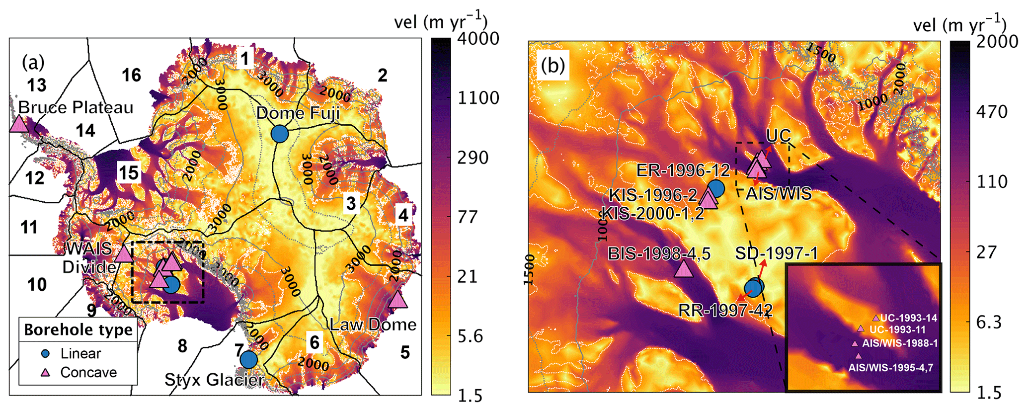
Figure 1 (a) Borehole locations with temperature measurements overlaid over ice velocity (Rignot, 2017). The dashed black box shows the location of (b). The solid black box in (a) indicates each basin from Jourdain et al. (2020), and each number indicates each basin number. We use a different symbol for each borehole based on the shape of its temperature profile (blue dots and magenta triangles indicate linear profiles and concave profiles, respectively). The gray contours indicate surface elevations, with dashed lines for every 500 m and solid lines for every 1000 m. The white-dot contours indicate regions where ice velocity is 10 m yr⁻¹. (b) Enlargement of borehole locations at West Antarctica overlaid over the ice velocity. The borehole names are abbreviated: WIS, Whillans Ice Stream; BIS, Bindschadler Ice Stream; ER, Engelhardt Ice Ridge; KIS, Kamb Ice Stream; RR, Raymond Ice Ridge; UC, Unicorn; AIS, Alley Ice Stream; and SD, Siple Dome.

Hondoh et al. (2002)Engelhardt (2004b)Engelhardt (2004b)Yang et al. (2018)Engelhardt (2004b)Engelhardt (2004b)Slawny et al. (2014)Van Ommen et al. (1999)Zagorodnov et al. (2012)Engelhardt (2004b)Engelhardt (2004b)Engelhardt (2004b)Engelhardt (2004b)Engelhardt (2004b)Engelhardt (2004b)

Table 1 Summarized information for each borehole. The observed ice velocity is from Rignot (2017), and the number in parentheses indicates error in magnitude of ice velocity. The date refers to when the boreholes were drilled.

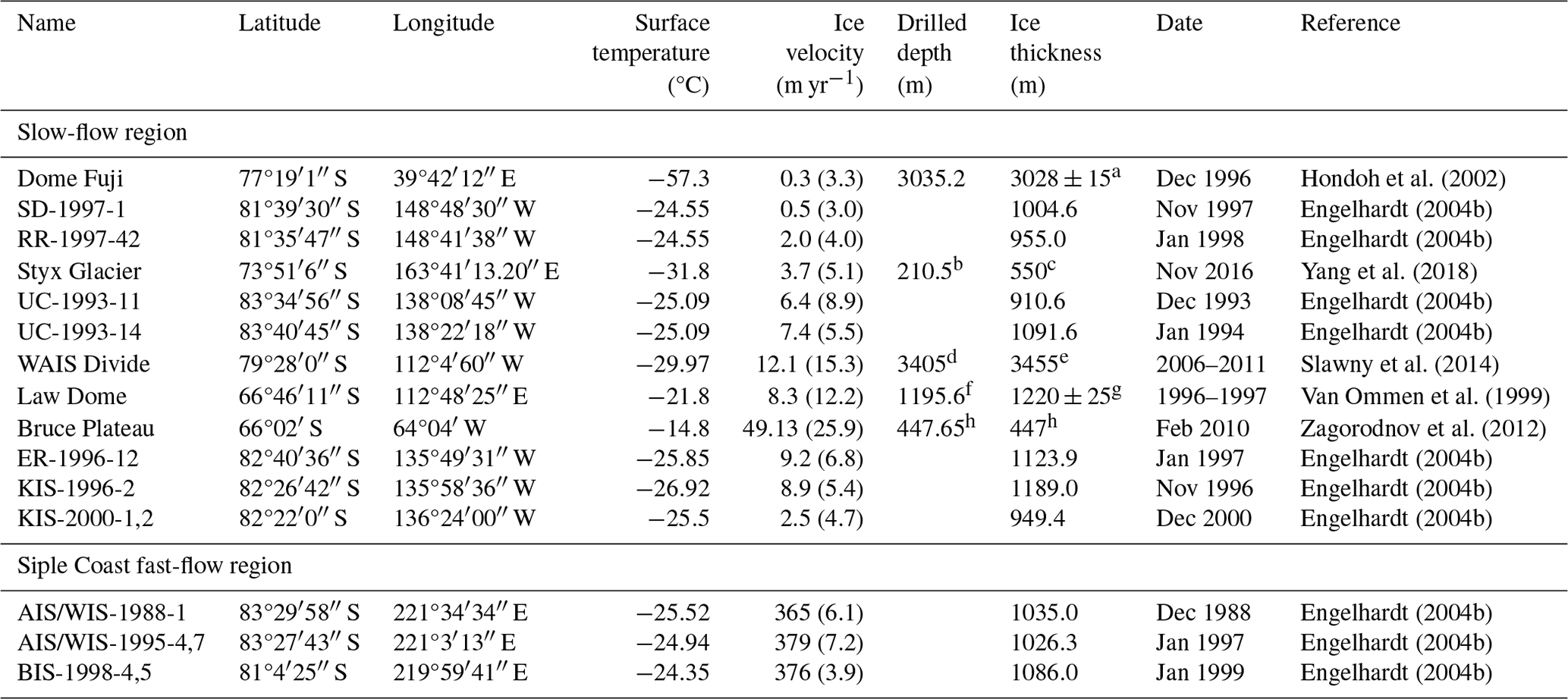
^a Parrenin et al. (2007). ^b Yang et al. (2018). ^c Hur (2013). ^d Slawny et al. (2014). ^e WAIS Divide Project Members (2013). ^f Morgan et al. (1997). ^g Zagorodnov et al. (2012).

Since the vertical distance between the temperature measurements along the borehole profile and the triangular mesh is not uniform, we calculate a weighted absolute misfit between the modeled and the measured temperatures (or modeled ice surface velocities) when evaluating the thermal model's performance:

$$\begin{array}{}\text{(6)}& \text{misfit}=\sum _{i=\mathrm{1}}^{n_{\mathrm{obs}}}{w}_{\mathrm{i}}\left|Y_{\mathrm{i}}^{\mathrm{mod}}-Y_{\mathrm{i}}^{\mathrm{obs}}\right|,\end{array}$$

where n_obs is the number of measured points at each borehole (or the number of observed ice velocities), i indicates the index of the specific measured elevation (or index of the ice velocity area), w_i is a weight calculated from the ratio of a specific measured point’s occupying length to the total measured length (or ratio of the measured area to the total area), and Y_i is the temperature (or ice velocity magnitude). The subscripts “obs” and “mod” indicate the observed and modeled variables, respectively.

Since the ice thickness and the surface temperature of the ice flow model are not always exactly consistent with the observed borehole data, we make adjustments using an exponential decaying correction following Pattyn (2010):

$$\begin{array}{}\text{(7)}& X_{\mathrm{corr}}=X+\left(X_{\mathrm{0}}-X\right)\exp \left(-{\displaystyle \frac{\sqrt{{\left(x-x_{\mathrm{w}}\right)}^{\mathrm{2}}+{\left(y-y_{\mathrm{w}}\right)}^{\mathrm{2}}}}{\mathit{\sigma }}}\right),\end{array}$$

where (x_w,y_w) is the location of the borehole, X₀ is the observed quantity, and X is the model ice thickness or surface temperature. The surface temperature at each borehole (except for SD-1997-1, RR-1997-42, UC-1993-11, AIS/WIS-1988-1, and BIS-1998-4,5) is corrected where the given climatological temperature is relatively higher than the observed surface temperature (Table 1). X_corr is the corrected data, and σ is the radius of influence, which is set here to 50 km. The geometry from BedMachine is constrained using radar-derived ice thickness measurements, except for at Dome Fuji and Law Dome, for which few thickness measurements were available. These two locations are the only places where an ice thickness correction is applied so that the ice thickness is 3090 m at Dome Fuji and 1220 m at Law Dome.

3 Results

3.1 Model experiments

To estimate the ice temperature of the entire Antarctic continent, we perform eight different experiments by combining two different vertical velocity profiles (IVz and IVz-nosliding) and four different GHF datasets. Table 2 shows the weighted absolute misfits between the modeled and observed surface ice velocities across the entire domain. The mean ice surface velocity misfit is 12.5 m yr⁻¹ for the IVz group and 19.5 m yr⁻¹ for the IVz-nosliding group. The standard deviation in the ice velocity misfit is 0.09 m yr⁻¹ for the IVz group and 0.35 m yr⁻¹ for the IVz-nosliding group.

Table 2 Experimental design for eight simulations using different vertical velocities and geothermal heat fluxes. The value between parentheses under each experiment represents the weighted absolute misfit between observed and modeled surface ice velocity across the entire domain.

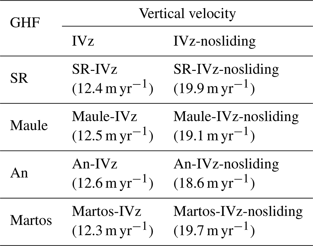
Figure 2 displays the measured and modeled vertical profiles of the ice temperature at the 15 borehole locations (see Fig. S1). The measured vertical profiles of the borehole temperatures, marked as dashed black lines in Fig. 2, can be categorized into two groups based on temperature profile shapes. One group exhibits concave profiles, for which the vertical advection toward the bed dominates, while the other group has a more linear shape, for which vertical diffusion dominates. Dome Fuji, SD-1997-1, RR-1997-42, ER-1996-12, and Styx Glacier at slow-flow regions show diffusion-dominant temperature profiles compared to the WAIS Divide, Bruce Plateau, Law Dome, KIS-1996-2, KIS-2000-1,2, UC-1993-11, and UC-1993-14, where the advection toward the bed dominates. Note that AIS/WIS-1991-1, AIS/WIS-1995-4,7, and BIS-1998-4,5 are located in regions with comparatively high ice velocity compared to other boreholes and have concave temperature profiles. To clearly define this specific fast-flow region, we refer to AIS/WIS and BIS as the Siple Coast fast-flow region.

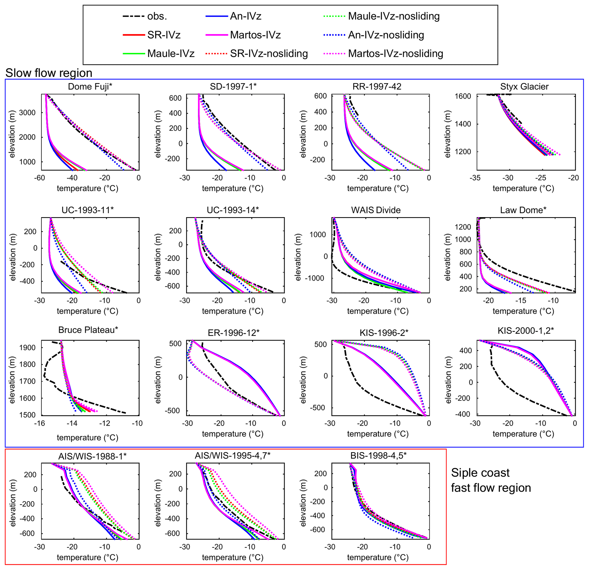
Figure 2 Observed and modeled vertical temperature profiles from eight different experiments at 15 borehole locations. Blue and red boxes indicate slow-flow and Siple Coast fast-flow regions, respectively. The bottom elevation at each borehole is set considering the ice thickness, as listed in Table 1. An asterisk next to the borehole name indicates that the drilling reaches the bedrock.

3.2 Borehole temperature profiles

To provide a quantitative comparison between the modeled and observed borehole temperatures, a weighted absolute misfit is calculated (Fig. 3). The average temperature misfit values for IVz and IVz-nosliding are 5.64 °C and 3.61 °C, respectively, and 1.69 °C and 2.50 °C for slow-flow and Siple Coast fast-flow regions, respectively. The temperature misfit value of the IVz-nosliding group is lower than that of the IVz group; however, the misfit temperatures in the Siple Coast fast-flow regions for IVz and IVz-nosliding are not exactly the same. The spread in misfits among the different vertical velocity schemes is larger than the one obtained when varying GHF. This shows that the difference in GHF has a limited influence on estimating the overall temperature profiles, while the choice of vertical velocities has a stronger impact. Both the IVz and IVz-nosliding groups demonstrate good performance in Siple Coast fast-flow regions, such as AIS/WIS and BIS. In the case of slow-flow regions, the thermal model's performance for the IVz-nosliding group is improved compared to the IVz group, and the model produces a reduced temperature misfit. However, none of the experiments successfully reproduce the temperature profiles at KIS boreholes, where the ice has been stagnant since around 1850 CE (Alley et al., 1994; Joughin and Tulaczyk, 2002). This history cannot be captured by our thermal steady-state assumption. A more detailed description of misfit values for each borehole can be found in the next section.

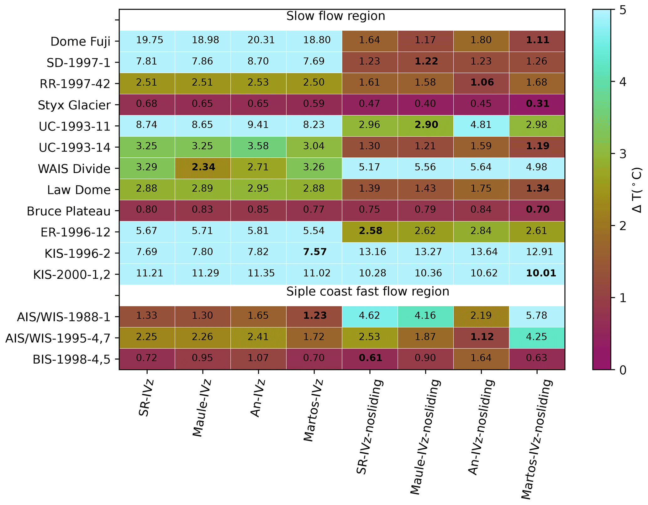
Figure 3 Weighted absolute misfit between observed and modeled borehole temperatures according to each experiment. The absolute temperature misfit is truncated over 5 °C.

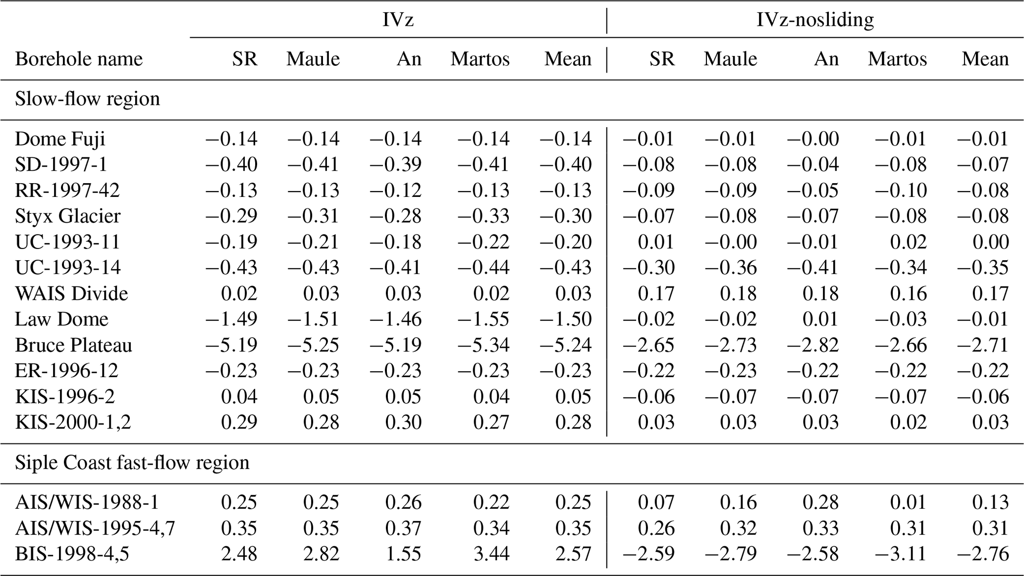
First, we focus on the three borehole profiles: SD, RR, and Dome Fuji. They all have linear temperature profiles, which are rarely observed in general borehole temperature profiles. SD and RR are adjacent to each other, but measurements of borehole temperatures at RR are limited to the top few hundred meters. Dome Fuji is located in the interior of the ice sheet. For these boreholes, the IVz group does not capture the linear shape of the temperature profiles. The IVz-nosliding group at these boreholes has a misfit value within 2 °C, which is lower than that of the IVz group (Fig. 3). The basal temperatures from the IVz-nosliding group reach the pressure melting point at SD, RR (Engelhardt, 2004b), and Dome Fuji. In the case of An, the GHF at each borehole is 40.1 mW m⁻² for Dome Fuji, 64.9 mW m⁻² for SD, and 65.3 mW m⁻² for RR, which is lower than the values from other GHF sources. The basal modeled temperature for An is the lowest and does not reach pressure melting point. The depth-averaged vertical velocity at Dome Fuji is −0.14 m yr⁻¹ for IVz (where a negative value means the vector is oriented downward), which is a higher value than that of IVz-nosliding (−0.01 m yr⁻¹) (Table 3). The depth-averaged vertical velocities of IVz at SD and RR are also higher than those of IVz-nosliding. This suggests a larger advection toward the ice sheet base in the IVz group, where downward heat advection is more dominant than the diffusion process and leads to a colder basal temperature compared to in the IVz-nosliding group.

Table 3 Depth-averaged vertical velocity for each experiment at each borehole. Positive values indicate upward advection.

At the borehole of Styx Glacier, both IVz and IVz-nosliding groups display similar average misfit values of ∼0.64 °C and ∼ 0.40 °C, which show good agreement with the observed temperature profiles. The drilling depth of Styx Glacier is about 210.5 m (Yang et al., 2018), and the ice thickness measured with a ground-penetrating radar survey is about 550 m (Hur, 2013). While we cannot definitively confirm the basal condition from observations, the thermal model results suggest that none of the glaciers reach the melting point.

The UC boreholes are located at an area of stagnant ice and have a relatively high basal temperature gradient compared to the other adjacent boreholes, such as the AIS/WIS boreholes (Engelhardt, 2004b). The mean GHF in the UC region is approximately 81.4 mW m⁻² for SR, 86.5 mW m⁻² for Maule, 62.8 mW m⁻² for An, and 95.6 mW m⁻² for Martos. The current modeled temperature profiles at UC-1993-11 and UC-1993-14 agree well with the measured temperature regardless of the choice of GHFs. The misfit value for the modeled and observed temperatures from the IVz-nosliding group is lower than that of the IVz group. In addition, the misfit of UC-1993-14 for IVz-nosliding is lower than that of UC-1993-11 (Fig. 3). UC-1993-14 is located in a slow region; however, UC-1993-11 is adjacent to the shear margin of the AIS ice stream, which induces a sharp transition in the basal velocity constraints for the IVz-nosliding group where the ice velocity crosses 10 m yr⁻¹. While the IVz-nosliding group better captures the observed temperature profiles for UC-1993-14, this is not the case for UC-1993-11.

The modeled basal temperature at the WAIS Divide reaches the pressure melting point for only the SR and Martos IVz groups. The GHF is approximately 112.6 mW m⁻² for SR and 141 mW m⁻² for Martos; these values are higher than those of the other two GHF datasets, which are 60.3 mW m⁻² for Maule and 68.9 mW m⁻² for An. The basal melting rate of the IVz-nosliding group is 7.9 mm yr⁻¹ for SR, 2.5 mm yr⁻¹ for Maule, 3.4 mm yr⁻¹ for An, and 10.9 mm yr⁻¹ for Martos. GHF estimations in previous studies are 113.3±16.9 mW m⁻² from Talalay et al. (2020) and 90.5 mW m⁻² from Mony et al. (2020). The thickness at WAIS Divide is 3455 m (WAIS Divide Project Members, 2013). However, the drilling depth is 3405 m (Slawny et al., 2014) and does not reach the bed, so we do not know the rate of basal melting. According to Talalay et al. (2020), the estimated basal temperature at WAIS Divide reaches the pressure melting point, and the basal melting rate is about 3.7±1.7 mm yr⁻¹. All experiments show reasonably good agreement in terms of the shape of the observed borehole temperature profile at WAIS Divide regardless of the choice of GHF. The average misfit value of the borehole temperature for IVz is 2.90 °C and is better than that of IVz-nosliding (Fig. 3).

At Law Dome, the misfit between the observed and modeled temperatures is 2.9 °C and 1.5 °C for the IVz and IVz-nosliding groups, respectively (Fig. 3). A primary difference between IVz and IVz-nosliding is the depth-averaged vertical velocity, the value of which is −1.5 m yr⁻¹ for the IVz group and −0.1 m yr⁻¹ for the IVz-nosliding group (Table 3). In the Law Dome case, we confirm that the use of IVz-nosliding improves the model’s vertical temperature profile (Fig. 2).

The observed ice velocity at Bruce Plateau is 49 m yr⁻¹ according to Rignot (2017), which is higher than the previously reported value of 10±4 m yr⁻¹ (Zagorodnov et al., 2012). We find that none of the modeled thermal profiles can reproduce the upper part of the observed ice temperature that captured the colder surface temperature of past climates (Zagorodnov et al., 2012). The mean vertical velocity for the IVz group is −5.24 m yr⁻¹ and is −2.71 m yr⁻¹ for the IVz-nosliding group; these values indicate high vertical advection toward the bottom.

With the exception of ER-1997-12, neither the IVz group nor the IVz-nosliding group captures the observed temperature profiles at the KIS boreholes. All modeled temperature profiles exhibit a convex shape (Fig. 2). At ER-1997-12, the mean misfit between the modeled and observed temperature is 2.7 °C for the IVz-nosliding group and 5.7 °C for the IVz group (Fig. 3).

The AIS/WIS and BIS boreholes are located in the fast-flow regions of the Siple Coast, where the ice velocities are 365 m yr⁻¹ for AIS/WIS-1991-1, 379 m yr⁻¹ for AIS/WIS-1995-4,7, and 376 m yr⁻¹ for BIS-1998-4,5 from Rignot (2017). The average misfit values of the IVz group are 1.38 °C for AIS/WIS-1988-1, 2.16 °C for AIS/WIS-1995-4,7, and 0.86 °C for BIS-1998-4,5 (Fig. 3). In these regions, both IVz and IVz-nosliding allow for basal sliding. However, there are differences in misfit values between IVz groups and IVz-nosliding groups at AIS/WIS. The reason for these differences is that the modeled ice velocities of IVz-nosliding in the AIS/WIS region are slower than the ones from IVz because it is a narrow ice stream that is influenced by the no-sliding constraint along its sides, resulting in higher misfit values for the IVz-nosliding group compared to the IVz group. The misfit between the modeled and observed temperatures at BIS is lower than that of AIS/WIS. In fast-flow regions, the advection, estimated through the stress balance of the ice and the ice incompressibility, plays a more important role in the thermal model than diffusion does. In these advection-dominated regions, the temperature is sensitive to bed geometry. A likely explanation for the difference in the misfits between the BIS and AIS/WIS regions is that the bed geometry in the BIS region is constructed using a mass conservation approach, which relies on the equation of ice incompressibility. In contrast, the bed geometry in the AIS/WIS region is constructed using the stream diffusion method, similar to kriging (Fig. S5). This suggests that enhancement in the quality of the geometry and utilizing the mass conservation method in the Siple Coast fast-flow regions would improve the estimation of the vertical velocity by the IVz equation with sliding and improve the overall performance of the thermal model. The AIS/WIS-1995-4,7 borehole is located at the center of the ice stream, whereas AIS/WIS-1988-1 is relatively near the margin of the ice stream. Although the bed geometry at AIS/WIS is constructed using the kriging method, IVz reproduces the temperature profile reasonably well at the center of fast ice flow regions.

3.3 Subglacial conditions

Figure 4a and b show the mean and the standard deviation of the basal temperature distribution for the eight experiments. The mean basal temperature at the main ice trunk, where the ice primarily discharges into the ocean, reaches the ice pressure melting point. The standard deviation of the basal temperature is higher in the internal ice compared to in the peripheral regions. In the case of IVz-nosliding, constraining the basal velocity to zero in slow-flow regions leads to a warmer basal temperature distribution compared to in the IVz group. In slow-flow regions, the basal temperature of the IVz group shows a notable difference depending on the choice of GHF. The modeled basal temperatures in the Maule and Martos experiments, which have higher mean GHF values (Table 4), are warmer than those in the SR and An experiments, as expected. The mean GHF of An is the lowest compared to the other GHFs, and, therefore, the basal temperature at each borehole modeled with the An GHF is lower than those of the other GHFs.

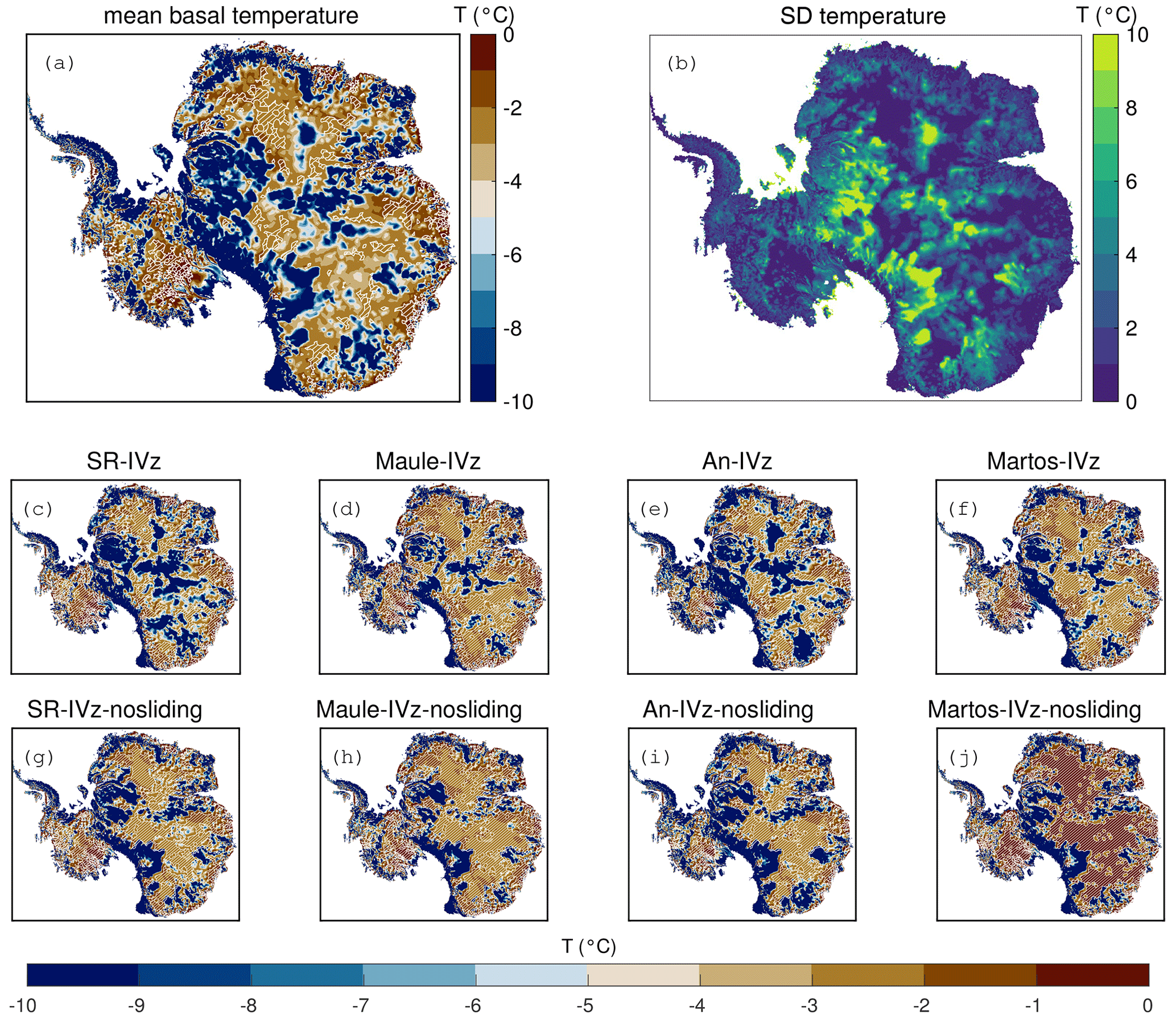
Figure 4 (a) Mean and (b) standard deviation of the basal temperature distribution from eight experiments. (c–j) Basal temperature distribution for each experiment. The temperature legend is truncated below −10 °C. A hatched region with a white line indicates that the basal temperature of ice reaches the pressure melting point.

All the experiments generally indicate that most of the regions experiencing basal melting are concentrated in fast-flow regions, where basal frictional heat is significant and provides enough heat for the ice to reach the pressure melting point (Fig. 4). Since IVz-nosliding displays lower vertical advection than that of IVz, the basal temperature of the IVz-nosliding group in slow-flow regions is warmer than that of the IVz group (Fig. 4c-j).

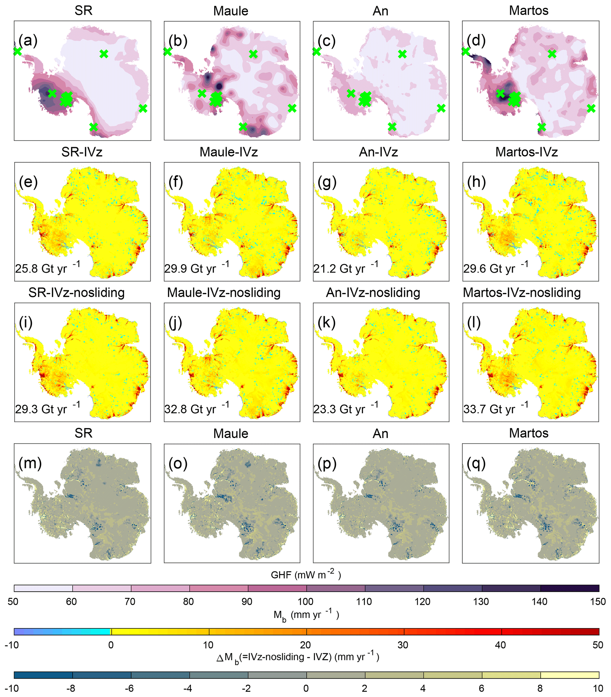
Figure 5 Upper panels (a–d) are the geothermal heat flux distributions of each source. Middle panels (e–l) are the basal melting rate distributions, with the value at the bottom left indicating the total grounded ice melting volume for each experiment. The basal melting rate exceeding 50 mm yr⁻¹ is truncated. Lower panels (m–q) are the difference in the basal melting rate between IVz-nosliding and IVz for each geothermal heat flux. The green crosses on the geothermal heat flux map indicate the borehole location. The color maps for the geothermal heat flux and the difference in basal melting rates are from Crameri et al. (2020).

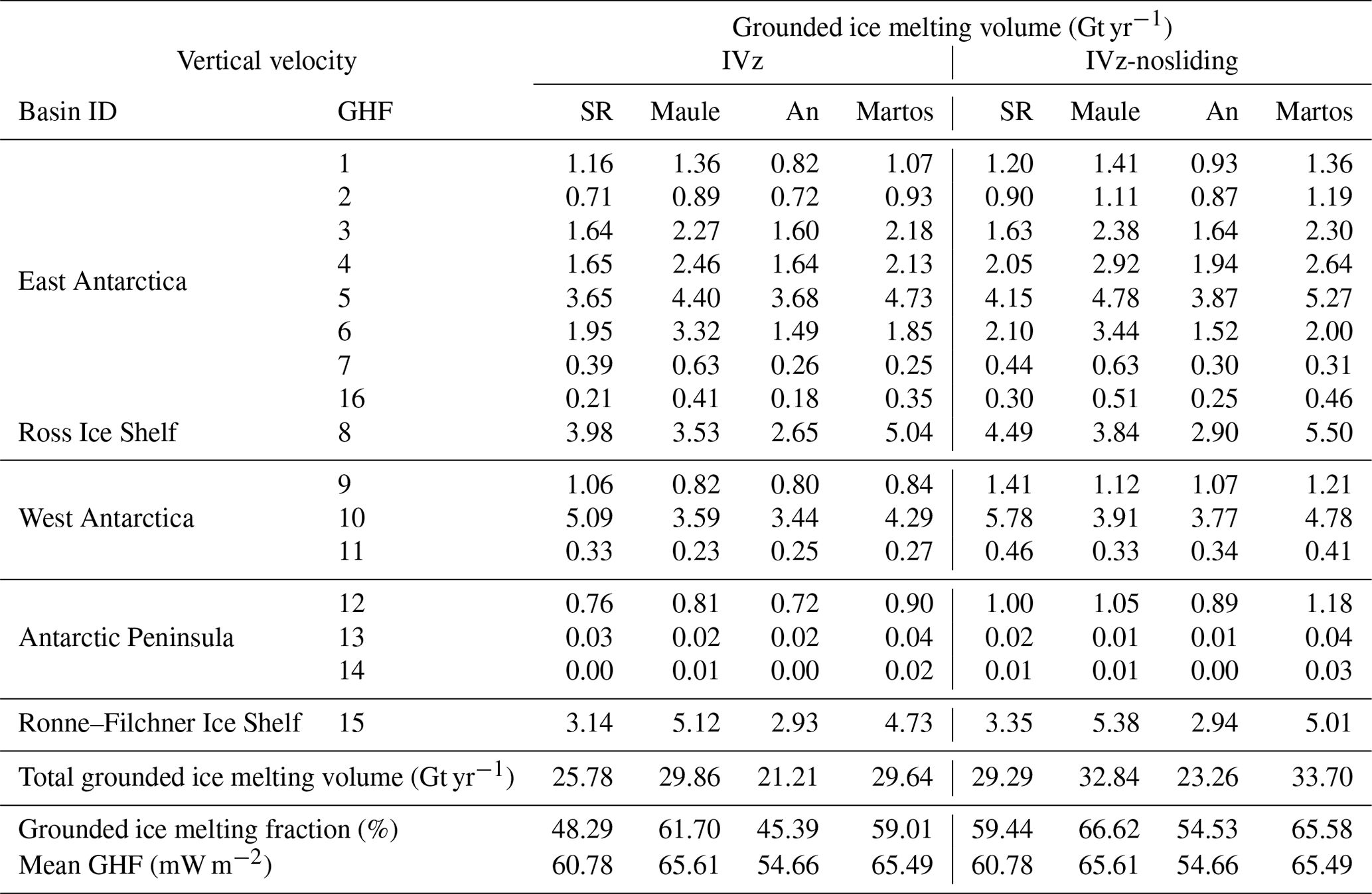
The mean total grounded ice melting volume is 26.62 Gt yr⁻¹ for the IVz group and 29.77 Gt yr⁻¹ for the IVz-nosliding group (Table 4). The total grounded ice melting volume for the IVz-nosliding group is 3.15 Gt yr⁻¹ higher than that of the IVz group. Compared to IVz, IVz-nosliding suggests a mean total basal melting volume increase of 1.89 Gt yr⁻¹ (60 %) and 1.26 Gt yr⁻¹ (40 %) in the slow-flow and fast-flow regions, respectively. The total grounded ice melting volume is proportional to the GHF magnitude. Each basin displays significant differences in terms of the grounded ice melting volume depending on the GHF source. Note that the GHF from An, which is the lowest value among all GHFs, shows the lowest total grounded ice melting volume.

Table 4 Grounded ice basal melting volumes of eight experiments at each basin (Fig. 1) and the total grounded ice melting volume and the total grounded melting fraction corresponding to each experiment.

4 Discussion

Previous studies that have successfully reproduced borehole temperature profiles using one-dimensional thermal analytical solutions have been limited to slow-flow regions (Joughin et al., 2003; Mony et al., 2020; Talalay et al., 2020). These studies have demonstrated good agreement between modeled and observed temperatures, which is expected given their simplicity and the tunability of the analytical solutions. One important tunable parameter is the analytical vertical velocities, which rely on ice surface mass balance (Hindmarsh, 1999; Joughin et al., 2003; Talalay et al., 2020). The choice of vertical velocity is a key factor in reproducing borehole temperature profiles. Uncertainties in the GHF have also been identified as a major factor in reproducing observed borehole temperature profiles (Talalay et al., 2020; Mony et al., 2020). On the other hand, some other studies have shown that uncertainties in the GHF have little influence on model performance in terms of ice dynamics (Larour et al., 2012a; Smith-Johnsen et al., 2020a) and simulating future projections (Schlegel et al., 2018; Smith-Johnsen et al., 2020b; Seroussi et al., 2013). Therefore, to test other factors, such as different GHFs and vertical velocities, which may affect the calculation of borehole temperatures, we use a three-dimensional thermomechanical model in order to account for both horizontal and vertical advection. We compare our calculated temperatures to observed borehole profiles in both fast-flow and slow-flow regions.

In slow-flow regions, we find that IVz-nosliding experiments show reasonably good agreement with the observed borehole temperature profiles. However, the three-dimensional thermal model occasionally estimates convex temperature profiles, which are not consistent with the observations, such as the KIS boreholes. Compared to other boreholes, the ice velocities at KIS and ER gradually decrease from upstream to downstream and coincide with the presence of a basal ridge (Price et al., 2001; Ng and Conway, 2004) (see also Fig. S2). In the past, the KIS and ER regions experienced faster ice flow, and the ice stream started to stagnate around 1850 CE (Alley et al., 1994; Joughin and Tulaczyk, 2002). There are hypotheses explaining the stagnation in the KIS region: the water piracy hypothesis (Alley et al., 1994) or the removal of basal water contributing to the loss of lubrication (Tulaczyk et al., 2000; Bougamont et al., 2003). This history results in colder temperatures in the upper part of the ice column, which contains ice that was deposited farther upstream where the surface temperature was lower than it is at the current location of the boreholes. This ice was then transported downstream to the current location (Hills et al., 2023). In model experiments, Bougamont et al. (2015) revealed changes in the tributaries at KIS and ER using a plastic till deformation friction law including a simple subglacial hydrology model. In contrast, we employ the Budd-type friction law and assume the effective pressure fully connected to the ocean part, not including changes in the effective pressure. The variation in effective pressures also changed the basal ice velocity in the Budd-type friction law. In addition, a selection of other types of friction laws, including Weertman (Weertman, 1974), Schoof (Schoof, 2005), and Coulomb (Tsai et al., 2015) types, also influences the initialization and future fate of ice (Brondex et al., 2017, 2019). Further investigation is required, such as the application of other types of friction laws or initialization with paleo spin-up, to better understand temperature profiles.

In Siple Coast fast-flow regions, Joughin et al. (2004) utilized a thermal model with vertical velocity derived from an analytical solution, which reproduced the observed borehole temperature profile of BIS-1998-4,5 with good agreement (UpD in Joughin et al., 2004). Here, we also find that the modeled temperature using a vertical velocity based on the equation of incompressibility without any constraint or tunable parameter also agrees well with the observed temperatures in this sector.

The total grounded ice melting volume for both the IVz and IVz-nosliding groups falls within the range reported by previous studies. It is lower than 65 Gt yr⁻¹ from Pattyn (2010) and higher than 14.7 Gt yr⁻¹ from Llubes et al. (2006). In the study by Joughin et al. (2009), a homogeneous GHF value of 70 mW m⁻² was adopted, which is similar to the mean GHFs from Maule (66.95 mW m⁻²) and An (67.15 mW m⁻²) at basin 10, which includes the Pine Island and Thwaites glaciers (see basin in Fig. 1). However, the total grounded ice melting mass estimated by Joughin et al. (2009) of 5.2 Gt yr⁻¹ is higher than that of the IVz group (average value of Maule and An) of 3.5 Gt yr⁻¹ and the IVz-nosliding group (average value of Maule and An) of 3.8 Gt yr⁻¹. The thermal models have been employed to explore the thermal regime of ice and to estimate basal melting rates beneath grounded ice. In the thermal model's advection term, the horizontal components of the ice velocity are estimated using the stress balance equations, whereas the vertical velocity is recovered from the ice incompressibility. Under kriging-based bed topography, the vertical velocity in fast-flow regions leads to large flux divergences (Seroussi et al., 2011). In contrast, mass-conservation-based bed geometries, such as BedMachine (Morlighem et al., 2017, 2020), preserve low flux divergence. We confirm that in areas where the bed geometry was inferred from mass continuity, the more accurate estimates of the vertical velocity provide a viable input for estimates of temperature profiles, for example, in the Siple Coast fast-flow regions. Additionally, we expect this study to provide a reliable understanding of temperature profiles in the other fast-flow regions generated with mass conservation. We should highlight that the good agreement between modeled and observed temperatures in fast-flow regions does not guarantee that the magnitude of basal melting volume is accurate, as it depends on both geothermal heat fluxes and frictional heat.

We find that the impact of using different GHF fields has only a modest influence on the ice temperature field and the total grounded ice basal melting volume. Under these circumstances, our results reveal that the shapes of the borehole temperature profile are less sensitive to the current estimated GHFs than previously reported. It is also worth noting that the initialization with the GHF from An results in underestimated basal temperatures and a lower total grounded ice melting volume due to an excessively low GHF value compared to other datasets.

The IVz-nosliding experiment has the advantage of better simulating the vertical temperature profiles in slow-flow regions compared to IVz. However, it tends to produce large discrepancies between modeled and observed surface ice velocities (Fig. S3). For instance, the An IVz-nosliding thermal model experiments exhibit the largest misfits in ice velocity among all the experiments, as the lowest value of average GHF leads to relatively high ice rigidity that perturbs the ice flow in the slow-flow regions. In contrast, the IVz experiment shows relatively smaller misfit values in surface ice velocity because sliding compensates for the underestimated internal deformations in the slow-flow region. In general, we find that IVz leads to a higher depth-averaged ice rigidity compared to IVz-nosliding in slow regions due to presence of colder ice temperatures (Fig. S4). Higher ice rigidity causes ice to deform less vertically, through vertical shear, and the surface ice velocity with no sliding cannot reproduce the observed surface velocities. In other words, the surface ice velocity of IVz-nosliding shows a larger ice velocity misfit compared to that of the IVz group, because the basal velocities are constrained to zero and cannot compensate for the high velocity misfit. Furthermore, the adoption of no sliding in specific regions results in a sharp transition zone in ice rigidity, B. This occurs because the basal velocity near the transition zone does not smoothly change from no sliding to sliding (Fig. S4). Therefore, additional work is required to address and resolve the smooth transition between no sliding and sliding.

In slow-flow regions, a competition between vertical diffusion and advection determines the shape of the temperature profiles and the bottom temperatures. In the IVz experiments, the boundary condition for basal vertical velocity is recovered with the gradient of the bed geometry and the basal melting volume. This approach provides relatively high vertical velocities in slow-flow regions. The vertical velocities are not always in agreement with the analytical expression of vertical velocities assuming a stationary bed and no sliding. As the depth-averaged vertical velocity of IVz is higher than that of IVz-nosliding, cold surface temperatures can be more effectively transferred deeper into the ice column.

The surface temperature of ice would be one of the factors in considering the boundary conditions of a thermal model. While ERA5 (Hersbach et al., 2023), RACMO2.3p2 forced with ERA5 (van Wessem et al., 2023), and MERRA-2 (Global Modeling and Assimilation Office (GMAO), 2015) are the recent reanalysis datasets, they display some discrepancies between the climatological mean 2 m air temperature (1980–2018) and the observed surface temperature at each borehole (Fig. S6). For the comparison with a different version of ECMWF (European Centre for Medium-Range Weather Forecasts) reanalysis data, we perform experiments in the same manner, utilizing 2 m air temperature from ERA5. These results display no significant differences compared to experiments using ERA-Interim (Fig. S7). However, in the case of SD, RR, and AIS/WIS (only for the IVz-nosliding case), they display slight discrepancies in surface temperature, leading to shifts in the modeled temperature profiles. In fact, the improvement in surface temperature and the accurate correction would bring the modeled temperatures into closer agreement with observations.

Finally, borehole temperatures have a long-term memory of past climate air temperatures and are a good proxy for reconstruction over a few hundred years or longer using inverse modeling (Nagornov et al., 2001; Zagorodnov et al., 2012). This history is not accounted for in this study, as we assumed thermal steady state using current climatological information. Despite this strong limitation, we find that this approach provides temperature profiles that are in good agreement with observations.

5 Conclusions

In this study, we used a three-dimensional thermomechanical model of Antarctica with different sources of GHF and vertical velocity fields to reproduce different thermal states of the Antarctic ice sheet, and we compared the results to 15 in situ measured borehole temperature profiles in slow-flow and fast-flow regions. Comparing the modeled to the measured borehole temperature profiles, we confirm that the vertical ice velocity based on the equation of incompressibility (IVz) is suitable for fast-flow regions, such as BIS, where the bed geometry is constructed using the mass conservation method, while an IVz that ignores basal sliding (IVz-nosliding) performs better in slow-flow regions. Our results show that the vertical temperature profile is more sensitive to the vertical velocity. In addition, the basal conditions, such as temperature and melting rate, are sensitive to both GHF and the vertical velocity field. The total grounded ice melting volume and basal temperature are proportional to the magnitude of the average GHF values for the same vertical velocity method. Finally, constraining the basal velocity to zero in slow-flow regions is a reasonable assumption and leads to a more realistic temperature profile.