Using specularity content to evaluate eight geothermal heat flow maps of Totten Glacier

Geothermal heat flow (GHF) is the dominant factor affecting the basal thermal regime of ice sheet dynamics. But it is poorly defined for the Antarctic ice sheet. We compare the basal thermal state of the Totten Glacier catchment as simulated by eight different GHF datasets. We use a basal energy and water flow model coupled with a 3D full-Stokes ice dynamics model to estimate the basal temperature, basal friction heat and basal melting rate. In addition to the location of subglacial lakes, we use specularity content of the airborne radar returns as a two-sided constraint to discriminate between local wet or dry basal conditions and compare the returns with the basal state simulations with different GHFs. Two medium magnitude GHF distribution maps derived from seismic modelling rank well at simulating both cold- and warm-bed regions, the GHFs from Shen et al. (2020) and Shapiro and Ritzwoller (2004). The best-fit simulated result shows that most of the inland bed area is frozen. Only the central inland subglacial canyon, co-located with high specularity content, reaches the pressure melting point consistently in all the eight GHFs. Modelled basal melting rates in the slow-flowing region are generally 0–5 mm yr⁻¹ but with local maxima of 10 mm yr⁻¹ at the central inland subglacial canyon. The fast-flowing grounded glaciers close to the Totten ice shelf are lubricating their bases with meltwater at rates of 10–400 mm yr⁻¹.

1 Introduction

Totten Glacier is the primary outlet glacier of the Aurora Subglacial Basin (ASB; Fig. 1) and one of the glaciers most vulnerable to a warming climate in East Antarctica (Li et al., 2016; Dow et al., 2020). It holds an ice volume equivalent of 3.9 m of global sea level rise (Morlighem et al., 2020; Greenbaum et al., 2015). Most of the bedrock below Totten Glacier is below sea level. The floating part, the Totten ice shelf, has a relatively high basal melt rate of ∼10 m yr⁻¹ compared with other ice shelves in East Antarctica (Rignot et al., 2013; Roberts et al., 2018) and has thinned and lost mass rapidly in recent years (Pritchard et al., 2009; Adusumilli et al., 2020).

The ASB has a widespread distributed hydrological network with almost 200 “lake-like” or water accumulation features (Wright et al., 2012; Livingstone et al., 2022). There may be a hydrological flow pathway operating from subglacial lakes near the Dome C ice divide and the coast via Totten Glacier (Wright et al., 2012), potentially affecting the stability of Totten Glacier.

Basal melting contributes to subglacial hydrological flow. Basal meltwater lubricates the flow of ice, which can impact the stability of the ice sheet and the direction of the ice flow (Livingstone et al., 2016; Bell et al., 2007). The basal meltwater moves down the pressure gradient and gradually develops into a complex subglacial hydrological system, which eventually flows into the ocean (Fricker et al., 2016). However, the spatial structure of the basal thermal state and basal melting rates beneath Totten Glacier are not yet well understood.

Basal melting can occur where the ice temperature reaches the pressure melting point, dramatically lowering the basal friction and allowing the ice to flow faster. Geothermal heat flow (GHF) is a key boundary condition for ice temperature. Its magnitude and distribution affect the distribution of basal ice temperature and thus the ice flow. The magnitude of GHF depends on the spatially varying geological conditions that control heat generation and conduction, including heat flow from the mantle, crustal thickness, heat production in the crust by radioactive decay, groundwater flow, and tectonic history (Pollack et al., 1993; Pittard et al., 2016; Reading et al., 2022). The bed topography affects heat diffusion pathways to the earth's crust and therefore has an influence on GHF at kilometre scales. Typically, the near-surface temperature gradient is decreased near topographic rises and increased near topographic depressions (Bullard, 1938; Colgan et al., 2021). It is difficult to measure GHF directly due to limited access to Antarctic bedrock, with only a few point measurements in ice-free areas or from boreholes through the ice (Fisher et al., 2015). GHF datasets are commonly estimated from models (Burton-Johnson et al., 2020) relying on either seismic models (Shapiro and Ritzwoller, 2004; An et al., 2015; Shen et al., 2020), magnetically derived models (Martos et al., 2017; Purucker, 2012 – an update of Fox-Maule et al., 2005), or a multivariate approach (Stål et al., 2021) including machine learning (Lösing and Ebbing, 2021).

Previous thermomechanical simulations of the whole Antarctic including Totten Glacier (Dow et al., 2020; Pattyn, 2010; Pittard et al., 2016; Van Liefferinge and Pattyn, 2013; Van Liefferinge et al., 2018) have used GHF data from Shapiro and Ritzwoller (2004), Fox Maule et al. (2005), Purucker (2012), and An et al. (2015), but Wright et al. (2012) and Huybrechts (1990) used spatially uniform values. In this study, we simulated the basal thermal state of Totten Glacier, based on the best available topographic data and eight different GHFs, including the three GHFs listed above, plus more recent GHF fields from Martos et al. (2017) and Shen et al. (2020), and the three latest GHF datasets from Stål et al. (2021), Lösing and Ebbing (2021), and Haeger et al. (2022).

We apply an off-line coupling between a basal energy and water flow model and a 3D full-Stokes ice flow model for each of the eight GHF maps to provide the best-fit distribution of the modelled basal temperature and basal melt rate. We evaluate the simulated basal temperature fields under the different GHF maps using the observations of water at the ice base to infer which GHF map is most reliable in the ASB. The observations include a set of subglacial lake locations and the specularity content (Dow et al., 2020) calculated from airborne radar data collected by the International Collaborative Exploration of the Cryosphere by Airborne Profiling (ICECAP) survey. Specularity is a parameterization of the along-track radar bed reflection scattering function that has been used to provide an attenuation-independent proxy for distributed subglacial waterbodies (Schroeder et al., 2013). We devise measures of specularity that help discriminate between alternative GHF maps to best characterize both cold and warm beds.

2 Regional domain and datasets

Our modelled domain, Totten Glacier, is located in the Aurora Subglacial Basin in East Antarctica (Fig. 1). Its boundary is based on drainage-basin boundaries defined from satellite ice sheet surface elevation and velocities (Mouginot et al., 2017). The surface elevation, bedrock elevation, and ice thickness are from MEaSUREs BedMachine Antarctica, version 2, with a resolution of 500 m (Morlighem et al., 2020).

Simulation input and comparison datasets are shown in Table 1. The surface ice velocity data are obtained from the MEaSUREs InSAR-Based Antarctica Ice Velocity Map, version 2, with a resolution of 450 m (Rignot et al., 2017), which were mainly collected during the International Polar Years from 2007 to 2009 with additional surveys between 2013 and 2016. Ice sheet surface temperature is prescribed by ALBMAP v1 with a resolution of 5 km (Le Brocq et al., 2010a) and comes from monthly estimates inferred from AVHRR data averaged over 1982–2004 (Comiso, 2000). Subglacial lake locations are from the fourth inventory of Antarctic subglacial lakes (Wright and Siegert, 2012) and the first global inventory of subglacial lakes (Livingstone et al., 2022).

Eight GHF datasets (Fig. 2; Table 2) are used in this study. Martos et al. (2017) GHF and Purucker (2012) GHF are both derived from magnetically derived models, but their magnitudes vary significantly on a regional scale, which is mainly related to the resolution of magnetic anomaly data (Burton-Johnson et al., 2020). Shapiro and Ritzwoller (2004), An et al. (2015), and Shen et al. (2020) all used seismic data, but they used different approaches in deriving heat flow. The latest three GHF datasets, Stål et al. (2021), Lösing and Ebbing (2021), and Haeger et al. (2022), are generated based on multiple observables. All the GHF datasets are bilinearly interpolated into 2.0 km resolution. Then we calculated the ensemble mean and standard deviation (SD) of the eight GHF maps and a uniform GHF value, 59 mW m⁻², which is the area average of the ensemble mean (Fig. 2). The SD of eight GHFs is less than 10 mW m⁻² over the domain.

The specularity content data are from Dow et al. (2020), where they calculated radar specularity content over the ASB from the ICECAP survey lines and smoothed the data with a 1 km filter, following the equations described in Schroeder et al. (2015). Specularity content is given as a relative value between 0 and 1, larger values mean a higher likelihood of water presence, and a value of 0.4 is taken as the division where specularity content shows the presence of water (Young et al., 2016).

Table 1 Datasets used in simulations.

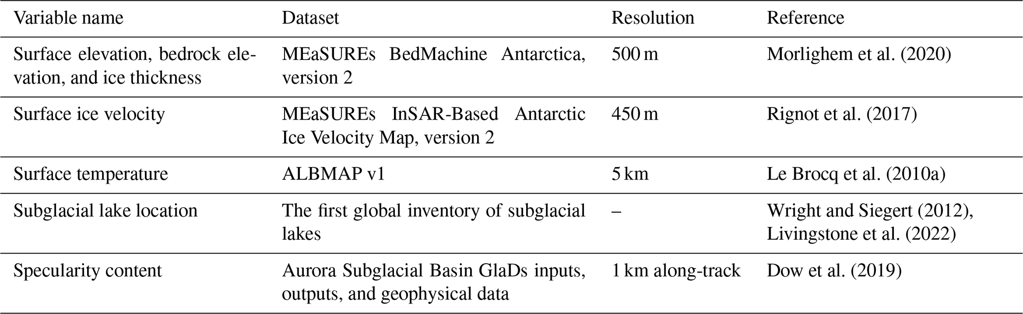
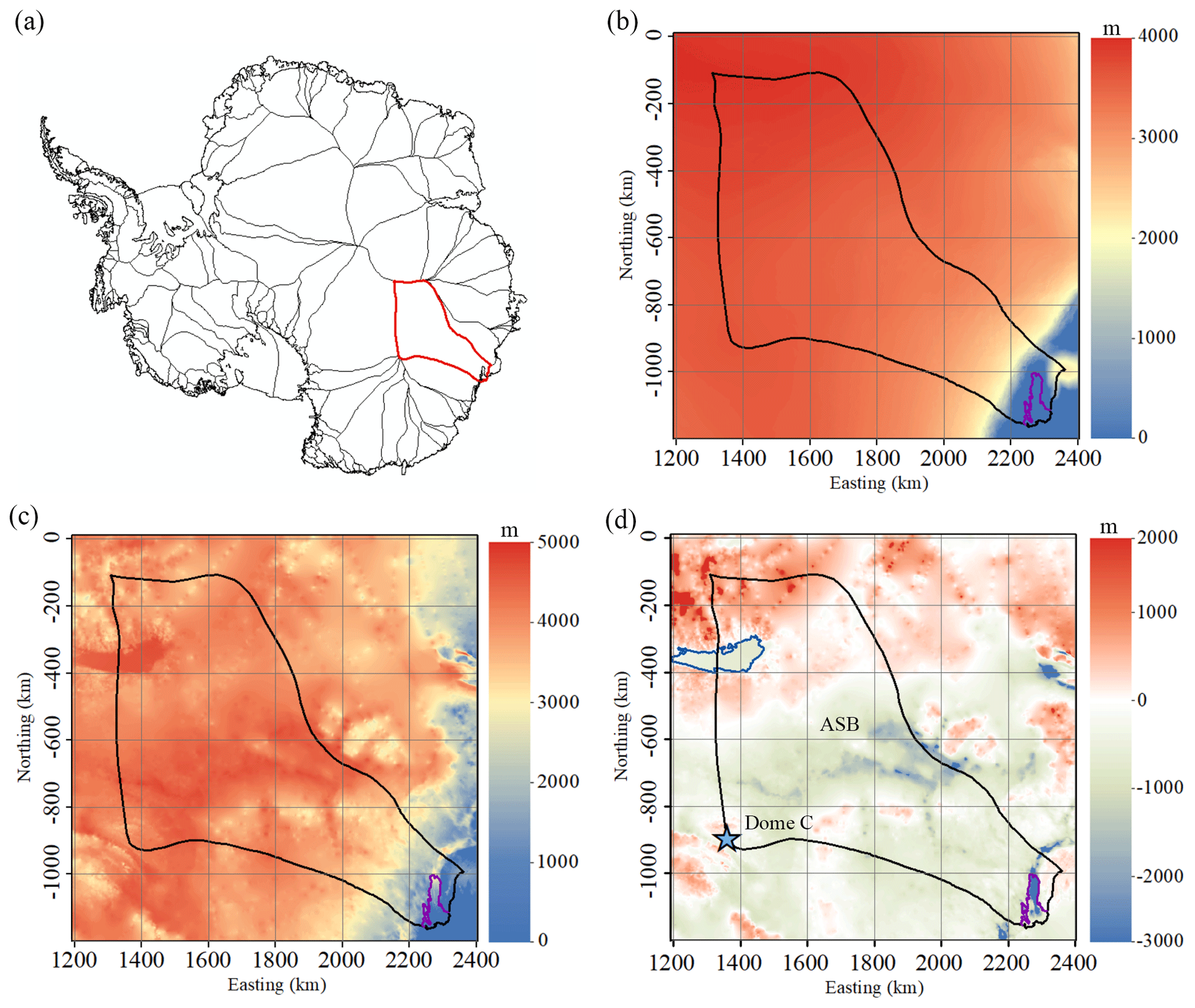
Figure 1 (a) The location of our domain in Antarctica; (b) surface elevation; (c) ice thickness; (d) bed elevation with region boundary overlain. The solid black curve is the outline of the study domain, including the Totten ice shelf. The solid red line in (a) is the boundary of Totten Glacier. The purple line in (b)–(d) depicts the grounding line of Totten Glacier. The blue curve in (d) depicts Lake Vostok (Studinger et al., 2003). The ASB and Dome C (blue star) are marked in (d).

Table 2 The 10 GHF maps used with the mean, range, and resolution in our region.

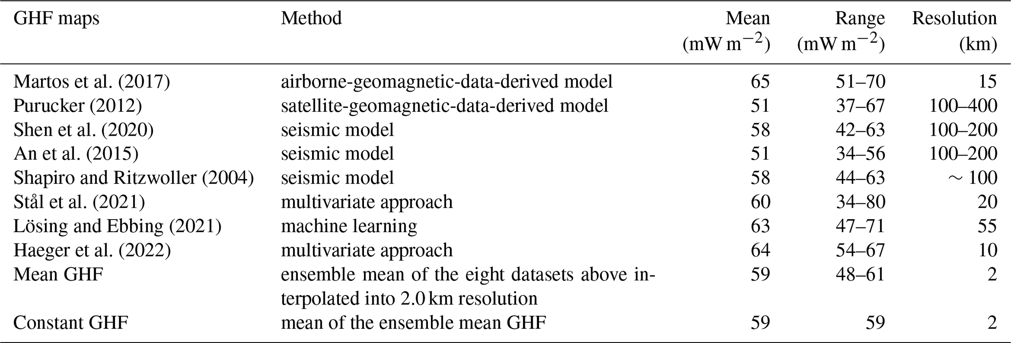
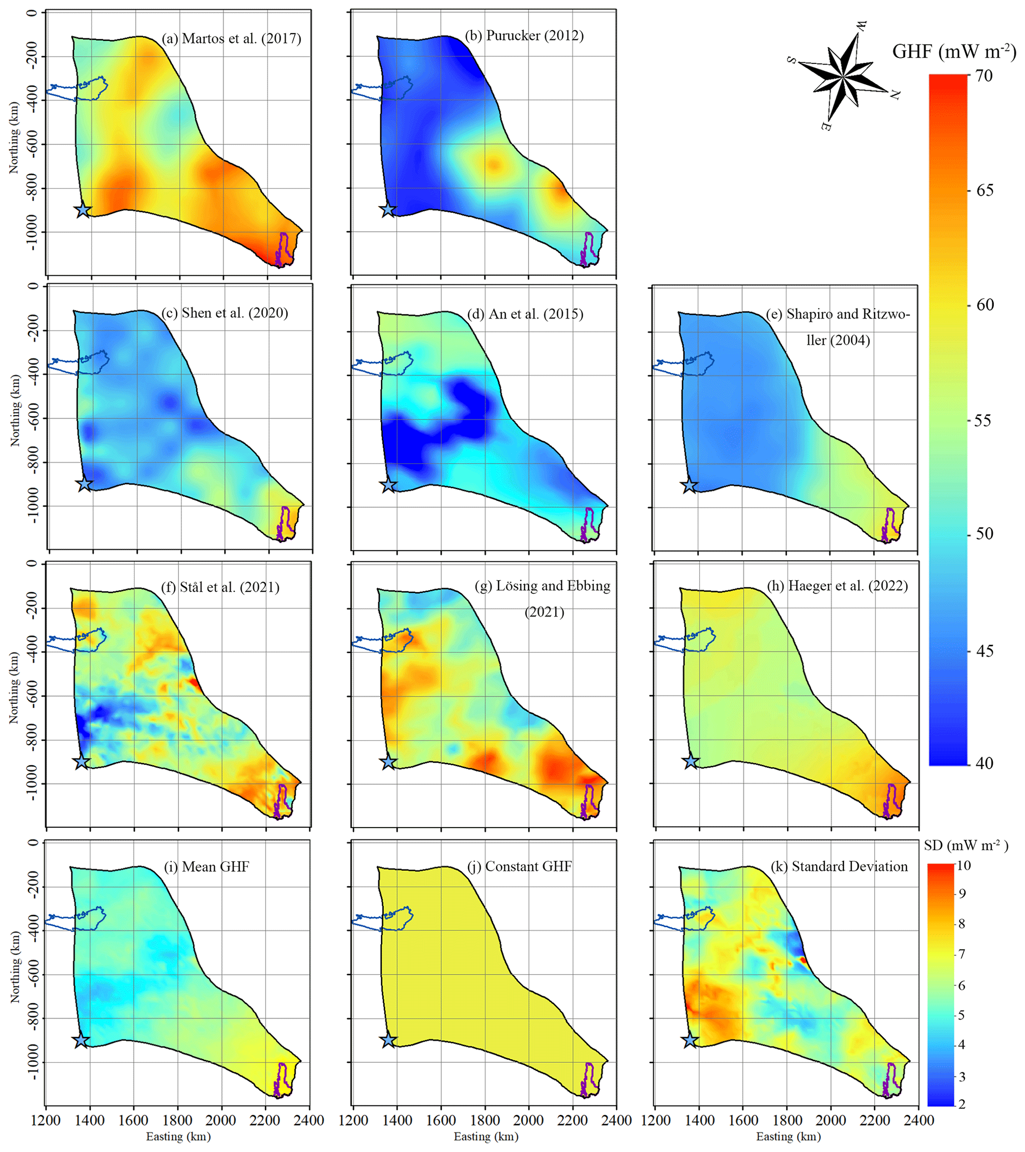
Figure 2 The spatial distribution of GHFs listed in Table 2 over our domain (a–j). The ensemble mean GHF and standard deviation of the eight GHFs (a–h) are given in (i) and (k). Panel (j) shows the constant GHF of 59 mW m⁻². The purple line depicts the grounding line. The blue curve depicts Lake Vostok. The blue star denotes Dome C.

3 Model

Our goal is to map the basal thermal state of Totten Glacier, including the basal temperature and basal melting rate. GHF, basal frictional heat, and englacial heat conduction are the main factors that determine the basal thermal state of the ice sheet. We need to simulate the ice flow velocity and stress to calculate the basal frictional heat and to simulate the ice temperature to calculate the englacial heat conduction flux.

Following the same method as Kang et al. (2022), we solve an inverse problem by a full-Stokes model, implemented in Elmer/Ice (Gagliardini et al., 2013), to infer the basal friction coefficient such that the modelled velocity best fits observations. To get a proper vertical ice temperature profile subject to thermal boundary conditions needed in solving the inverse problem, we use a forward model that consists of an improved shallow-ice approximation (SIA) thermomechanical model with a subglacial hydrology model (Wolovick et al., 2021). We perform steady-state simulations by coupling the forward and inverse models, using eight GHF datasets, as well as the ensemble mean GHF and a constant GHF value of 59 mW m⁻² (Fig. 2).

3.1 Mesh generation and refinement

We use Gmsh (Geuzaine and Remacle, 2009) to generate an initial 2D horizontal footprint mesh. Then we refine the mesh by an anisotropic mesh adaptation code in the Mmg library (http://www.mmgtools.org/, last access: 24 December 2023). The resulting mesh is shown in Fig. 3 and has minimum and maximum element sizes of about 800 m and 20 km. The range of the mesh size is 800 m at the ice shelf, 1–3 km upstream near the grounding line, and 6–20 km over most of the inland ice. The 2D mesh is then vertically extruded using 10 equally spaced, terrain-following layers.

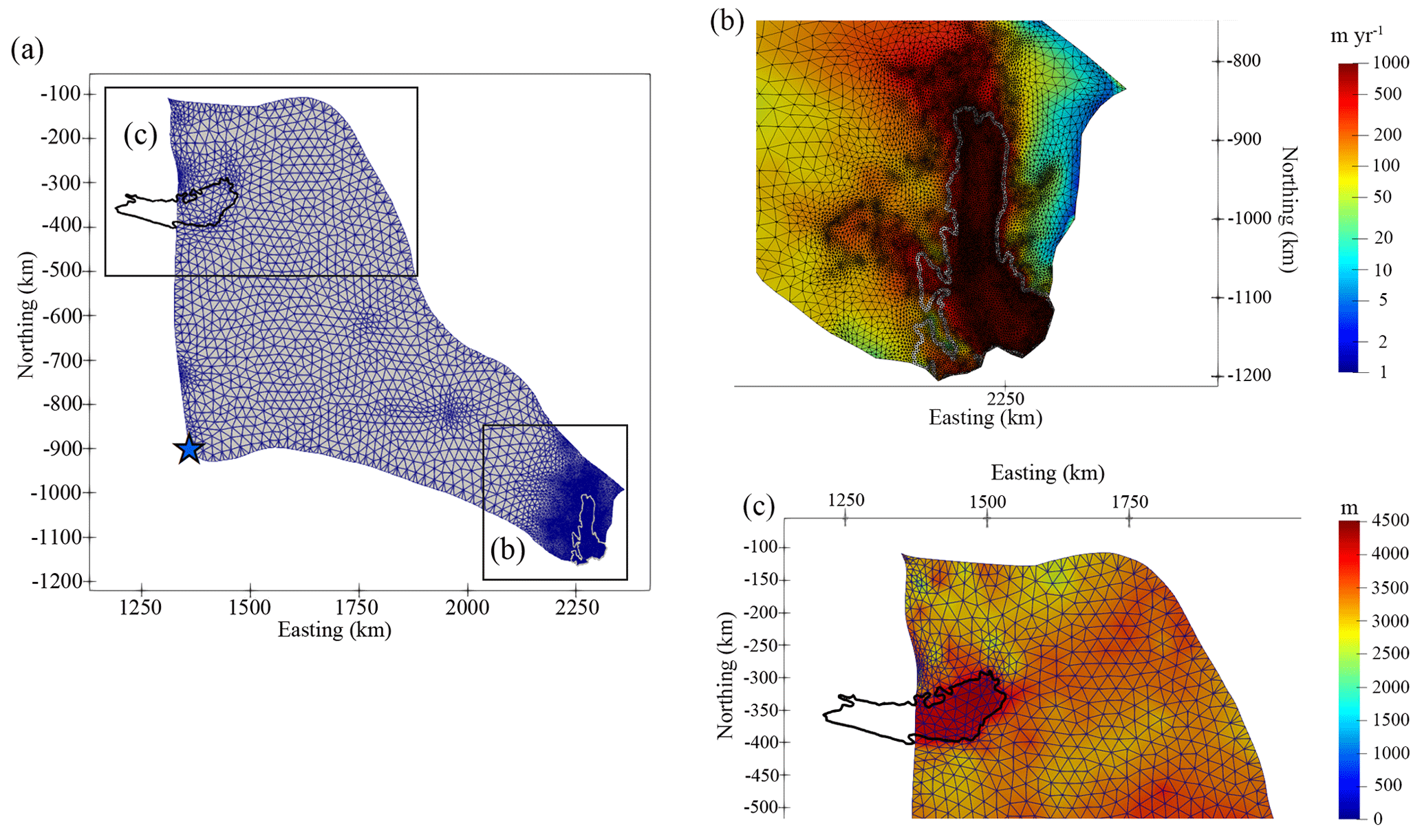
Figure 3 The refined 2D horizontal domain footprint mesh (a). Boxes outlined in (a) are shown in detail overlain with surface ice velocity (unit: m yr⁻¹) in (b) and with ice thickness in (c). The white line in (a) and (b) depicts the grounding line. The black curve in (a) and (c) depicts Lake Vostok. The blue star in (a) denotes Dome C.

3.2 Boundary conditions

The ice surface is assumed to be stress-free. At the ice front, the normal stress under the sea surface is equal to the hydrostatic water pressure. On the lateral boundary, the normal stress is equal to the ice pressure applied by neighbouring glaciers and the normal velocity is assumed to be 0. The bed for grounded ice is assumed to be rigid, impenetrable, and fixed over time. For simplicity, we ignore the existence of Lake Vostok and replace the lake with bedrock. We do this to avoid having to implement a spatially variable sea level in our model, as the level of hydrostatic equilibrium in Lake Vostok is several thousand metres higher than in the ocean. Our inverted drag coefficient over the lake is very low, indicating that our simplification has only a small influence on ice flow. However, our basal melt rates over the lake are probably inaccurate, as we assume that geothermal flux from the lake bottom is applied directly to the ice base, without accounting for circulation within the lake.

A linear sliding law is used to describe the relationship between the basal sliding velocity and the basal shear force, on the bottom of grounded ice:

$$\begin{array}{}\text{(1)}& {\mathit{\tau }}_{\mathrm{b}}=C\cdot u_{\mathrm{b}}.\end{array}$$

To avoid non-physical negative values, C=10^β is used in the simulation. We call β the basal friction coefficient. C is initialized to a constant value of 10⁻⁴ MPa m⁻¹ yr⁻¹ (Gillet-Chaulet et al., 2012) and then replaced with the inverted C in subsequent inversion steps.

We relax the free surface of the domain by a short transient run to reduce the non-physical spikes in initial surface geometry (Zhao et al., 2018). The transient simulation period here is 0.5 years with a time step of 0.01 years.

Following the same method as Kang et al. (2022), we improve the parameterization of β via C by considering basal temperature T_bed:

$$\begin{array}{}\text{(2)}& {\mathit{\beta }}_{\mathrm{new}}={\mathit{\beta }}_{\mathrm{old}}+\mathit{\alpha }\left(T_{\mathrm{m}}-T_{\mathrm{bed}}\right),\end{array}$$

where β_old is from the inverse model, α is a positive factor to be tuned and T_m is the pressure melting temperature. We take α to be 1 and use the parameterization of β_new in Eq. (1) in all the simulations (Kang et al., 2022). Using Eq. (2) does not change simulated surface velocities in the interior region.

3.3 Basal melt rate

Based on the inverted basal velocity and basal shear stress, we can calculate the basal friction heat. We then produce the basal melt rate using the thermal equilibrium as follows (Greve and Blatter, 2009):

$$\begin{array}{}\text{(3)}& M={\displaystyle \frac{G+{\mathit{u}}_{\mathrm{b}}{\mathit{\tau }}_{\mathrm{b}}+k\left(T\right)\frac{\mathrm{d}T}{\mathrm{d}z}}{{\mathit{\rho }}_{\mathrm{i}}L}},\end{array}$$

where M is the basal melt rate, G is GHF, u_bτ_b is the basal friction heat, $-k\left(T\right)\frac{\mathrm{d}T}{\mathrm{d}z}$ is the upward heat conduction, ρ_i is the ice density, and L is the latent heat of ice melt. GHF and frictional heating from basal slip warm the base, while the upward heat conduction to the interior cools the base.

4 Simulation results

4.1 Ice velocity

The modelled surface velocity fields with different GHFs are all very close to the observed as expected by design of the minimization of misfit between the modelled and the observed surface velocity in the inverse model. Therefore, we show only the Martos et al. (2017) result as a representative example of all simulated velocity fields (Fig. 4). The surface speed can reach as high as about 1000 m yr⁻¹ on the ice shelf (Fig. 4a, b).

Figure 4c shows the modelled basal ice velocity, which is close to 0 in most of the inland region. The fast basal velocity in the middle of the region (Fig. 4c) is associated with subglacial canyon features (Fig. 1c), high basal temperature (Fig. 5), and a small friction coefficient. In the grounded fast-flow region, the basal ice velocity can reach a maximum of 500 m yr⁻¹.

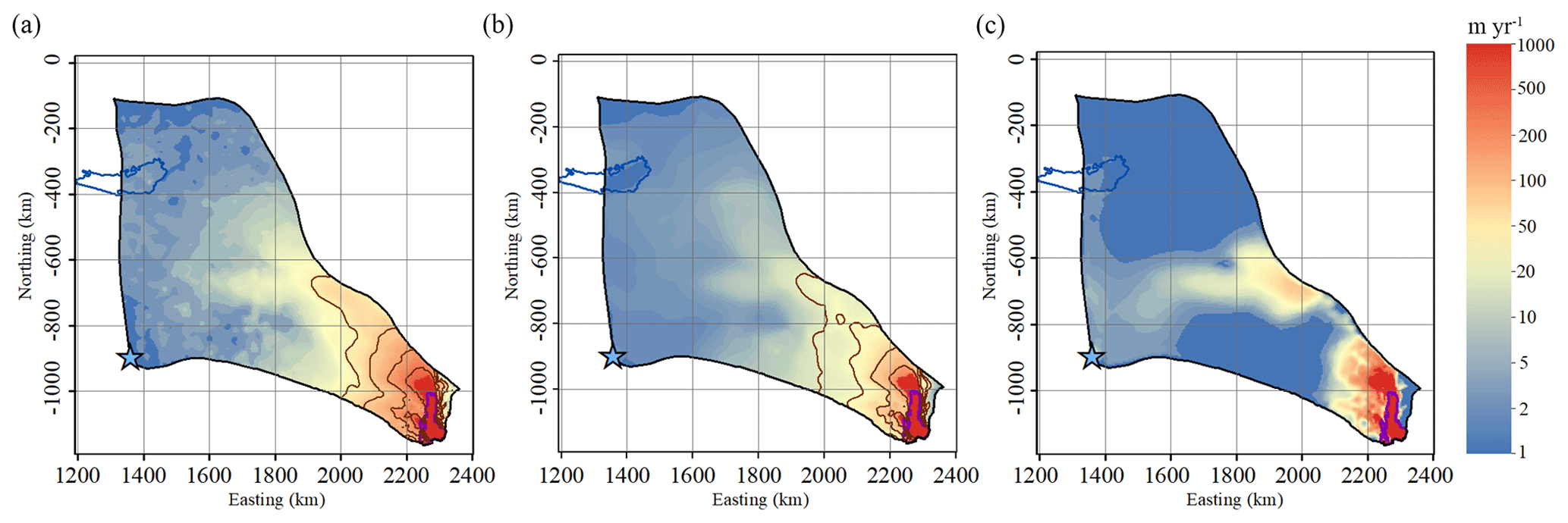
Figure 4 (a) Observed surface velocity, (b) modelled surface velocity, and (c) modelled basal velocity in the experiment using the Martos et al. (2017) GHF. The solid brown lines in (a) and (b) represent speed contours of 30, 50, 100, and 200 m yr⁻¹. The purple line depicts the grounding line. The blue curve depicts Lake Vostok. The blue star denotes Dome C.

4.2 Basal ice temperature, basal friction heat and heat conduction

Figure 5 shows the modelled basal temperatures from the 10 experiments. In the fast-flowing region (defined as having surface speeds higher than 30 m yr⁻¹), the modelled ice basal temperatures are all at the pressure melting point (“warm”). However, in the slow-flowing region, the modelled ice basal temperature shows large difference between GHF fields. In the experiment using the Martos et al. (2017), Haeger et al. (2022), Stål et al. (2021), and Lösing and Ebbing (2021) GHFs (Fig. 5), which have similarly high GHFs over the domain, we get the largest area of warm base extending to all but the inland southwest corner. The warm bed yielded by the constant GHF is close to the four abovementioned GHFs, although the constant GHF value is lower than the mean value of any one of the four abovementioned GHFs (Table 2). The experiment using Shen et al. (2020) GHF (Fig. 5c), which has a moderately high GHF, yields a medium-sized area of warm base. The experiments using An et al. (2015), Shapiro and Ritzwoller (2004), and Purucker (2012) GHFs produce slightly less area of warm bed than the Shen et al. (2020) GHF. The experiment using Purucker (2012) GHF (Fig. 5b), which is the lowest GHF, has the smallest warm base area, which is mostly confined to the fast-flowing region. All experiments show cold basal temperatures in the southwest corner, which is associated with relatively thin ice above subglacial mountains (Fig. 1c), and coincide with high values of SD in modelled basal temperature (Fig. 5k). The warm-bed area using the ensemble mean GHF is between that using the top four high GHFs and the GHF of Shen et al. (2020).

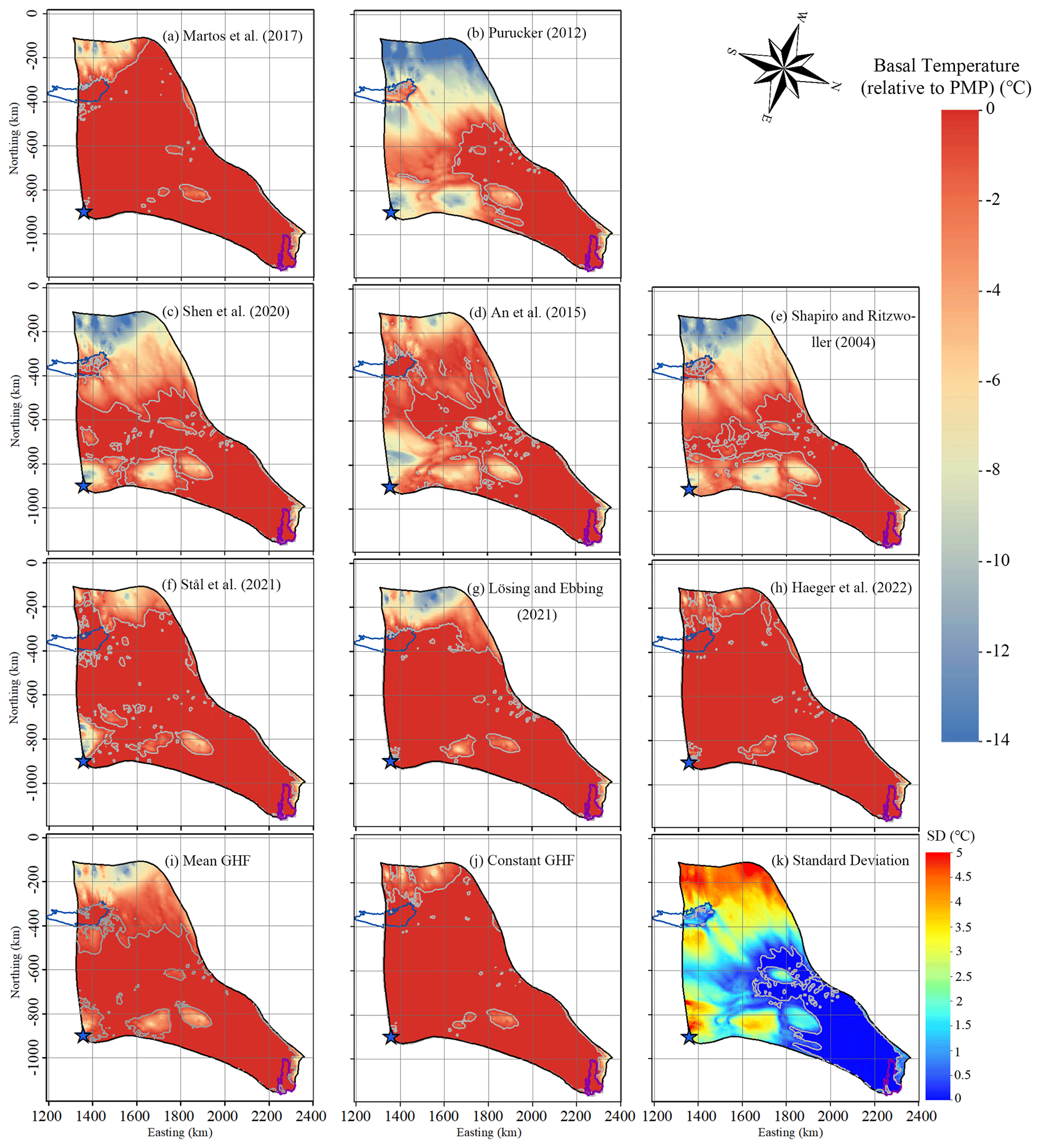
Figure 5 Modelled basal temperature relative to the pressure melting point (PMP), with (a) to (j) corresponding to the GHFs (a–j) in Fig. 2. Panel (k) is the standard deviation of eight modelled basal temperatures (a–h). The ice bottom at the pressure melting point is delineated by a grey contour. The purple line depicts the grounding line. The blue curve depicts Lake Vostok. The blue star denotes Dome C.

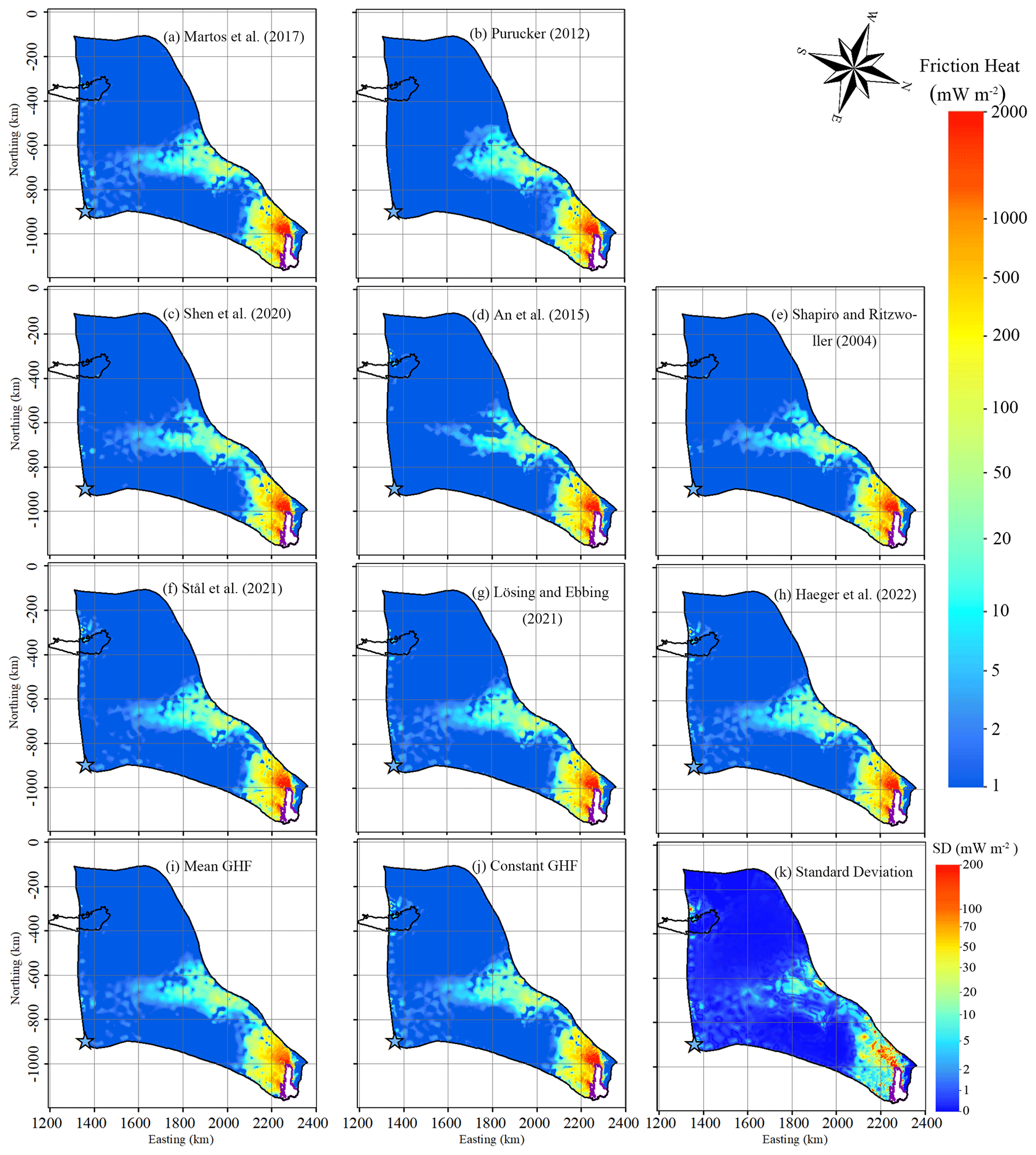
Figure 6 Modelled basal friction heat, with (a) to (j) corresponding to the GHFs (a–j) in Fig. 2. Panel (k) is the standard deviation of eight modelled basal friction heat results (a–h). The purple line depicts the grounding line. The black curve depicts Lake Vostok. The blue star denotes Dome C.

The distribution of modelled basal friction heat is closely associated with that of modelled basal velocity. The patterns of basal friction heat with different GHFs are very similar in fast-flow regions but have some differences in the middle of the domain (Fig. 6), where modelled basal velocity ranges between 5–20 m yr⁻¹ (Fig. 4).

The modelled basal friction heat is close to 0 where the surface ice velocity is less than 10 m yr⁻¹ but ranges widely by 10–2000 mW m⁻² with SD between 1 and 200 mW m⁻² in the fast-flowing region. Basal friction heating larger than 100 mW m⁻² occurs where surface velocity is more than 50 m yr⁻¹ and basal velocity is higher than 10 m yr⁻¹ (Figs. 6, 4), and it is then the dominant heat source.

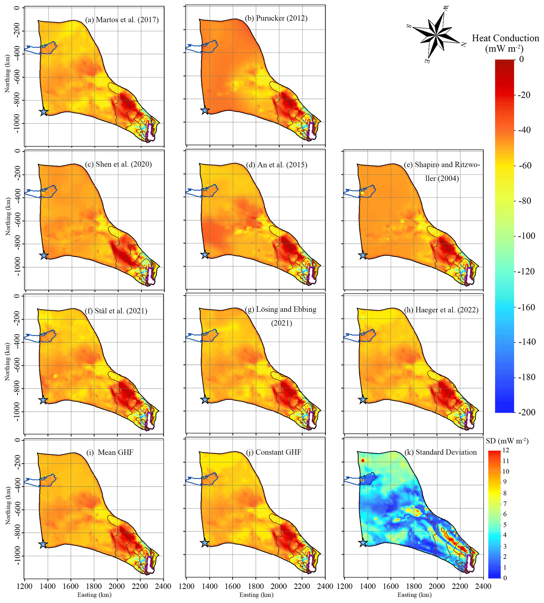
Figure 7 Modelled heat change in basal ice by upward englacial heat conduction. The negative sign means that the upward englacial heat conduction causes heat loss from the basal ice as defined by the colour bar, with cooler colours representing more intense heat loss by conduction. Panels (a) to (j) correspond to the GHFs (a–j) in Fig. 2. Panel (k) is the standard deviation of eight modelled upward englacial heat conduction results in basal ice (a–h). The solid brown curves represent modelled surface speed contours of 30, 50, 100, and 200 m yr⁻¹, as in Fig. 4. The purple line depicts the grounding line. The blue curve depicts Lake Vostok. The blue star denotes Dome C.

Figure 7 shows the modelled heat change in basal ice by upward englacial heat conduction in the 10 experiments. In the slow-flowing region where basal temperature is below the pressure melting point, the upward basal heat conduction equals the GHF (Figs. 5, 7). In the fast-flowing region with thick ice (≥2500 m; Fig. 1c), the heat loss caused by upward basal heat conduction is <30 mW m⁻² in all experiments (Fig. 7), reflecting the development of a temperate basal layer that limits the basal thermal gradient. In the fast-flowing tributaries with ice thickness <2000 m, the combination of reduced ice thickness and increased concentration of shear heating at the basal plane rather than in the lower ice column removes the temperate layer and allows very large values of upward basal heat conduction, up to 60–200 mW m⁻² near the grounding line (Fig. 7).

4.3 Basal melt rate

We calculate the basal melt rate using the thermal balance equation (Eq. 3). There are significant differences in the 10 experiments due to large variability in GHF (Fig. 8). The Martos et al. (2017), Haeger et al. (2022), Stål et al. (2021), and Lösing and Ebbing (2021) GHFs yield the largest areas with basal melting. The experiments using Shen et al. (2020), An et al. (2015), Shapiro and Ritzwoller (2004), and Purucker (2012) GHF yield smaller and similar total basal melting areas but have different spatial patterns. The basal melting area produced by the experiment using the ensemble mean GHF is between the four large areas and the four small areas. But the basal melting area produced by the constant GHF is larger than that by all the eight GHFs (Fig. 8).

In most of the warm-based regions, the modelled basal melting rate is <5 mm yr⁻¹ (Fig. 8) and basal friction heat is <50 mW m⁻² (Fig. 6). Basal melting rates >5 mm yr⁻¹ occur with surface velocities >100 m yr⁻¹ (Figs. 4, 8), where the basal friction heat is the dominant heat source. In particular, the modelled basal melting rate is 50–400 mm yr⁻¹ in the two fast-flow tributaries feeding the ice shelf that have surface velocities >200 m yr⁻¹ and where the basal friction heat can reach 500–2000 mW m⁻² (Figs. 4, 6, 8). This is consistent with the findings of Larour et al. (2012) and Kang et al. (2022), which indicate that the slow-flowing ice is more sensitive to GHF while the fast-flowing region is more sensitive to basal friction heat.

There is a relatively high modelled basal melt rate (4–10 mm yr⁻¹) localized at the central subglacial canyon (Figs. 8, 1c), which is captured by all 10 GHF experiments and is also consistent with the high values (0.5–1.0) of specularity content data there (Fig. 9). Dow et al. (2020) found that the specularity content is a useful proxy for both water depth and water pressure in regions of distributed water in subglacial canyons.

There is a location with modelled refreezing (negative melting rate) at the central subglacial canyon, near the observed subglacial lake, in all 10 GHF experiments (Fig. 8). The value of specularity content there is as low as 0–0.1 (Fig. 9), and freeze-on is driven by the steep topography around the canyon.

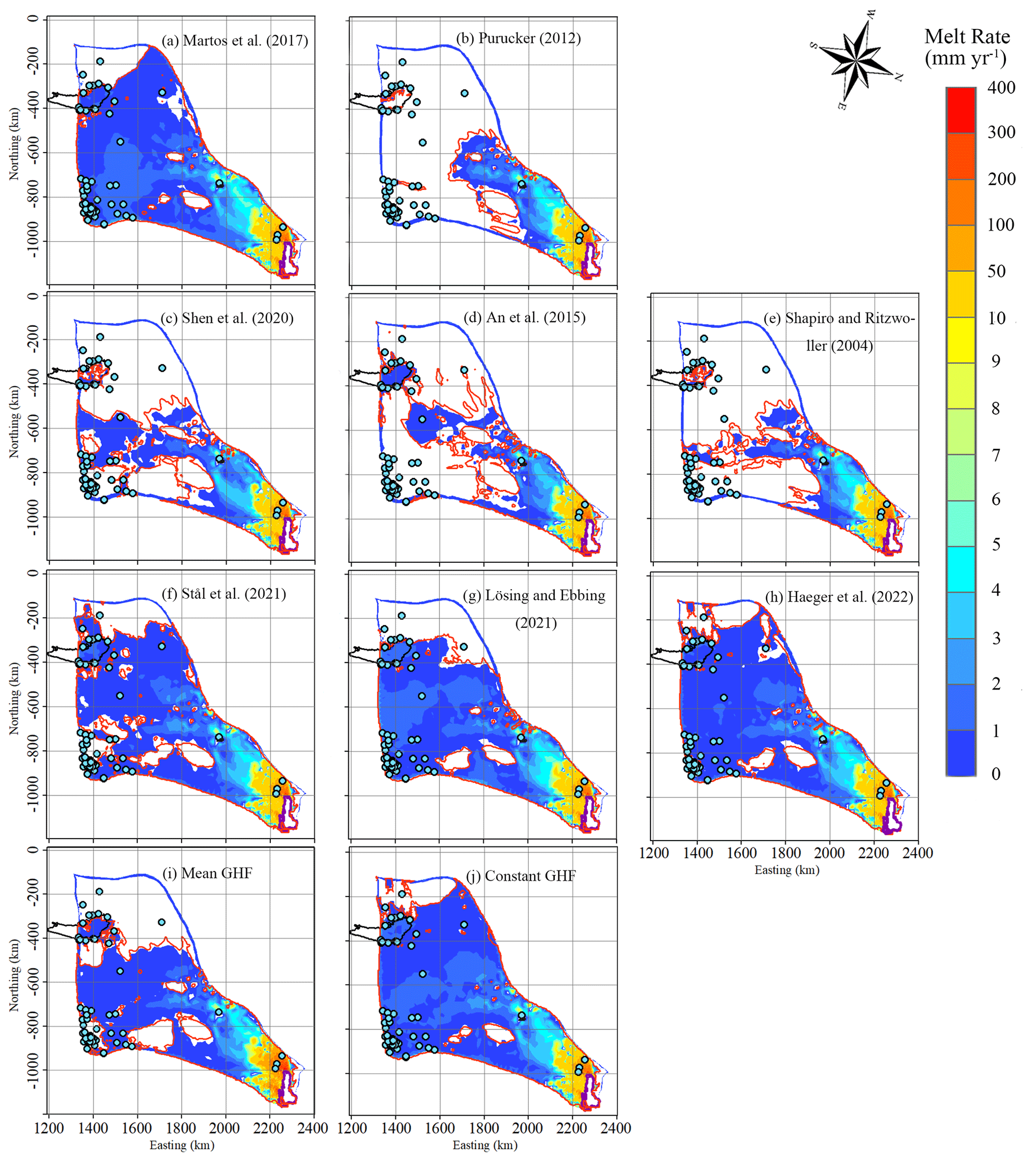
Figure 8 Modelled basal melt rate, with (a) to (j) corresponding to the GHFs (a–j) in Fig. 2. The ice bottom at the pressure melting point is surrounded by a red contour. The black curve depicts Lake Vostok. Stable subglacial lakes are shown as blue-green points with black circles. The purple line depicts the grounding line. There is modelled basal refreezing at the central canyon painted in black.

4.4 Evaluation of modelled results with eight GHFs

We use the locations of the observed subglacial lakes and specularity content to discriminate between modelled basal melting (Fig. 8). Ideally, we would like to have a modelled ice base that is cold and dry where subglacial lakes do not exist and the specularity content is low and a modelled ice base that is at the melting point where lakes and high specularity content are observed. In other words, we would like to use the available data to form a two-sided constraint that can penalize the model for being both too warm and too cold. If we only had a one-sided constraint, then we would always end up concluding that either the warmest or the coldest GHF map is best, regardless of whether that map was a reasonable representation of the basal state.

Observations of subglacial lakes are mostly a one-sided constraint on the basal thermal state. This is because lakes are only detectable if subglacial water accumulates in depressions that are deep compared to the radar wavelength and wide in comparison to the horizontal resolution of the radar system. Other forms of distributed hydrology, such as linked cavities or saturated subglacial sediments, do not produce the classic flat bright reflectors characteristic of subglacial lakes. Thus, the lack of observed subglacial lakes in a particular region cannot be taken as evidence that there is no subglacial water there. The mesh resolution of our model inland is about 20 km (Fig. 3). But 84 % of the subglacial lakes have along-radar track lengths below 5 km and 94 % are below 10 km, with only five lakes including Lake Vostok being above 10 km (Fig. 9f). So the subglacial lakes may be too small for the ice model to resolve. Nonetheless, we compare our modelled basal thermal state with the observed locations of subglacial lakes. These comparisons show that all the experiments can capture all four subglacial lakes in the fast-flowing region (Fig. 8). But their performance in covering subglacial lakes in the slow-flowing region differs greatly.

In addition to the subglacial lakes, we use specularity content to derive a two-sided constraint on the basal thermal state. Specularity content is an inherently noisy measure, so it is smoothed to 1 km along-track values, and furthermore it is not unambiguously an indicator of wet beds. For example, specularity content is low in the fast-flowing region (Figs. 9, 4), where there must be lubricating water at the bed. Similar specularity results were also seen by Schroeder et al. (2013) for Thwaites Glacier, where high specularity values are seen under the major tributaries and the upstream trunk but significantly lower values of specularity are seen in the fast-flowing region. This counter-intuitive result may be due to distinct morphologies and radar scattering signatures between water distributed in widespread subglacial conduits and water concentrated in just a few subglacial channels. Because of this effect, we only use the specularity content outside the fast-flowing region (defined as surface speed >30 m yr⁻¹, Fig. 9).

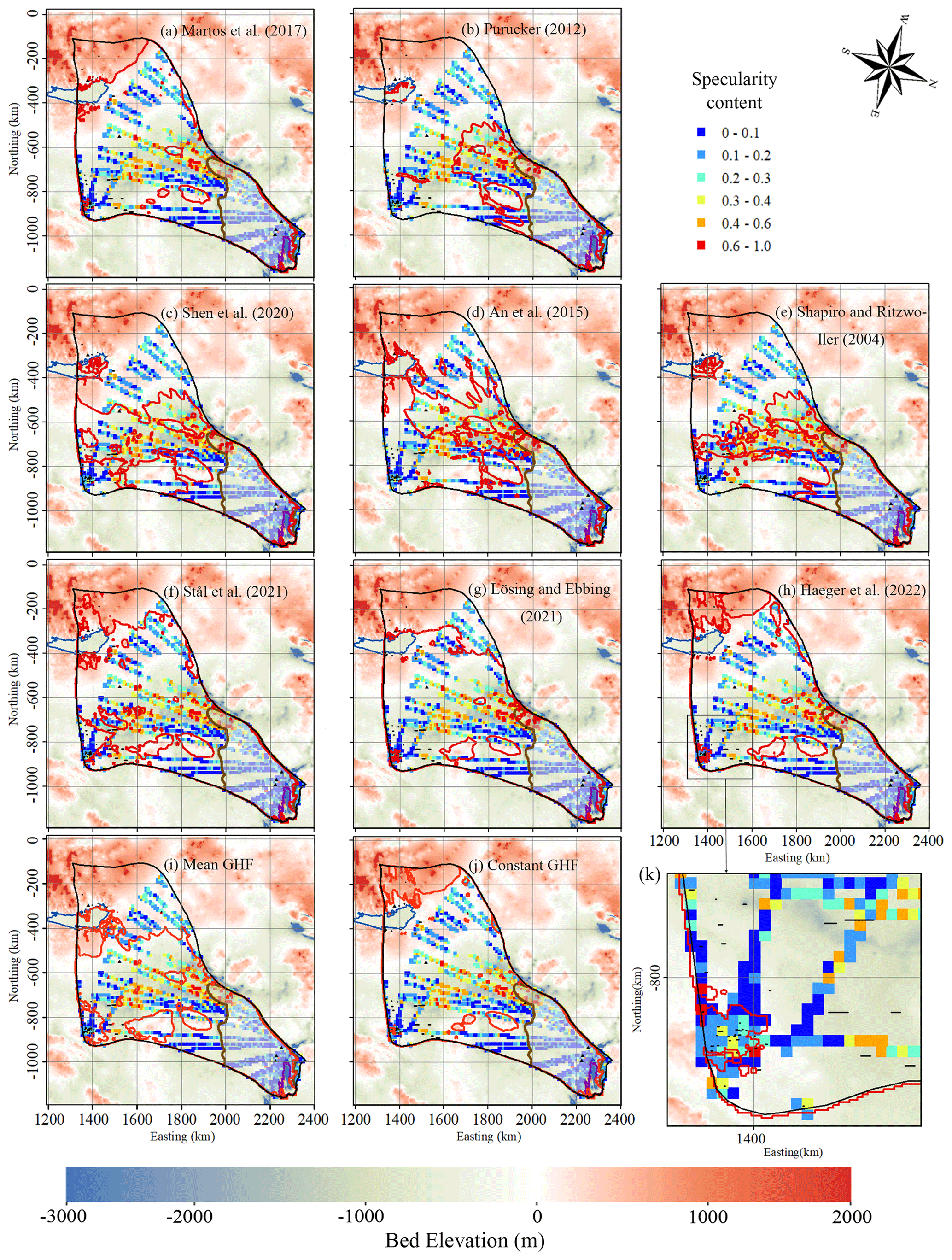
Figure 9 Locations of specularity content (coloured points) derived from radar data collected by ICECAP (Dow et al., 2020) and interpolated to 10 km by 10 km grids against the background of bedrock elevation. Specularity content >0.4 indicates the likely presence of basal water. The ice bottom at the pressure melting point is surrounded by a red contour; (a) to (j) correspond to the 10 GHF maps (a–j) in Fig. 2. Lake Vostok is outlined by a blue curve. The brown curve is the contour of the surface speed of 30 m yr⁻¹. Subglacial lakes are shown at observed positions as a line segment of their length. Plot (k) is an enlargement of the box in plot (h).

The specularity content data calculated from ICECAP survey lines suggest hundreds of locations with basal water (Dow et al., 2020). The default resolution of specularity content along the flight lines is 1 km (Dow et al., 2020), which is smaller than our model resolution of 6–20 km in the slow-flowing region. Water may accumulate in just a small fraction of the grid cell even if the majority of the cell is warm because of water flow. For comparability with our simulation resolution, we aggregated the specularity content data onto 10 km by 10 km windows (Fig. 9). The 10 km window is a somewhat arbitrary choice, but smaller windows (we tried 2 and 5 km) reduce the data available and noise becomes larger, while larger windows (we tried 15 and 20 km) restrict spatial resolution. We then take the upper fifth percentile of the specularity content, specularity₅, of each window as a water indicator rather than its mean value to allow for localized water collection or unfavourable bed reflection geometry while also excluding spurious signals in the noisy specularity data. Young et al. (2016) suggested that specularity larger than 0.4 was an indicator of a warm bed. This is also consistent with the largest subglacial lake in the domain with a length of 28 km having specularity content >0.4 (Fig. 9k). There are also some smaller lakes (along-track lengths of several kilometres) with specularity content between 0.2 and 0.4, so a warm threshold of 0.4 would not capture these features. The cold threshold need not be the same as the warm-bed one, and so we explored different values for cold thresholds of 0.2, 0.3, and 0.4, but we found that the 0.2 cold threshold provided the best discrimination between models and also maximized the available data.

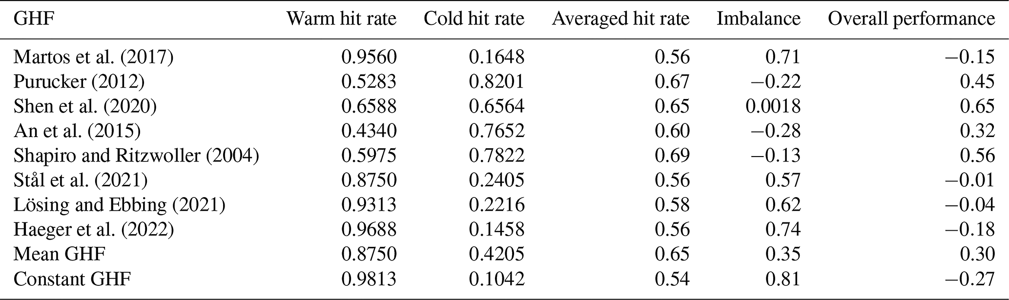
To evaluate modelled basal conditions with specularity content, we define a warm hit rate as the ratio of the number of grid cells with modelled warm bed that have specularity₅>0.4 to the total number of grids with specularity₅>0.4. Similarly, the cold hit rate is defined as the ratio of the number of grid cells with specularity₅<0.2.

One simple measure of quality is just the average of the warm hit rate and cold hit rate, but we also want an unbiased evaluation of GHF to have similar capabilities in capturing both warm-bed and cold-bed regions. Therefore, we define imbalance as follows:

$$\text{imbalance}={\displaystyle \frac{\text{warm hit rate}-\text{cold hit rate}}{\text{warm hit rate}+\text{cold hit rate}}},$$

as it reflects the difference between the warm hit rate and cold hit rate and has a value between −1 and 1. The closer to zero imbalance is, the more confidence we have in the model result. The overall performance is estimated by the averaged hit rate minus the absolute value of imbalance.

The constant GHF yields a higher warm hit rate and a lower cold hit rate compared to any single GHF map since it produces larger warm-bed area. The four highest GHFs, Martos et al. (2017), Haeger et al. (2022), Stål et al. (2021), and Lösing and Ebbing (2021) GHFs have similarly the highest warm hit rate and lowest cold hit rate among the eight GHFs since they have the largest modelled warm-bed area. The averaged hit rates of modelled results with eight GHFs are close, with differences <0.13 (Table 3). The Shapiro and Ritzwoller (2004), Purucker (2012), and then Shen et al. (2020) have the highest averaged hit rate using all the values for the threshold of cold bed, and the differences between their averaged hit rate are <0.04. The mean GHF has the same averaged hit rate as Shen et al. (2020).

Martos et al. (2017), Haeger et al. (2022), Stål et al. (2021), and Lösing and Ebbing (2021) GHFs have large positive imbalance >0.5, which means that their warm hit rates overwhelm their cold hit rates. Shen et al. (2020) have positive but near-zero imbalance.

In contrast, An et al. (2015), Shapiro and Ritzwoller (2004), and Purucker (2012) GHFs have negative imbalance (Table 3).

Considering the overall performance by the averaged hit rate minus the absolute value of imbalance, Shen et al. (2020) ranks the first, Shapiro and Ritzwoller (2004) the second, Purucker (2012) the third, and An et al. (2015) the fourth; Martos et al. (2017), Stål et al. (2021), Lösing and Ebbing (2021), and Haeger et al. (2022) get negative scores and rank as the last four among the eight GHFs (Table 3). The ensemble mean GHF gets a score close to An et al. (2015). The constant GHF gets a lower score than any GHF. The ranking is robust with all three cold hit thresholds.

Table 3 The warm hit rate, cold hit rate, averaged hit rate, imbalance, and overall performance for the modelled results with eight individual GHF maps, the ensemble mean GHF, and the constant GHF of 58.75 mW m⁻² in Table 2. The overall performance is calculated by averaged hit rate minus the absolute value of imbalance. The threshold of specularity₅ is taken as 0.4 for the warm hit rate and 0.2 for the cold hit rate.

5 Discussion

Wright et al. (2012) modelled basal temperature of Totten Glacier using the Glimmer ice sheet model with a constant GHF of 54 mW m⁻². Their modelled area of basal warm ice is between what we simulated using Martos et al. (2017) and Shen et al. (2020) GHFs, covering most of the lakes and lake-like features but missing some near Lake Vostok. Dow et al. (2020) ran the Ice Sheet System Model (Larour et al., 2012) with a constant GHF of 55 mW m⁻², producing a warm-bed region slightly larger than we simulated using the Shen et al. (2020) GHF (which has a mean of 58 mW m⁻² in this region, Table 2). However, our experiment with a constant GHF of 59 mW m⁻² produces a warm-bed region almost as large as that with the Martos et al. (2017) GHF, suggesting this constant value is too high for this domain. Our experiment with the ensemble mean GHF gives a warm-bed region close to that by the Shen et al. (2020) GHF, indicating the ensemble mean is a better choice than the mean of the ensemble mean.

Kang et al. (2022) evaluated basal thermal conditions underneath the Lambert–Amery glacier system using six GHFs and found that the two most recent GHF fields inverted from aerial geomagnetic observations and which have the highest GHF values produced the largest warm-based area and best matched the observed distribution of subglacial lakes. This might be expected as there was only a one-sided constraint used, and warm-based models produced matches with more lakes.

Although the basal ice in fast-flowing regions is all at the pressure melting point because basal friction heat dominates the heat balance, the modelled basal melt rate of the grounded ice in fast-flowing regions exhibits large differences across models. The modelled basal melt rate is associated with the modelled basal friction heat, which is a function of the modelled basal velocity and basal shear stress, the accuracy of which depends on the configuration and constraints of the ice sheet model used. Our modelled maximum basal melt rate on the grounded ice is 0.4 m yr⁻¹ near the grounding line. This is close to the modelled maximum basal melt rate of 0.34 m yr⁻¹ near the grounding line by Dow et al. (2020), where they calculated the basal melt rates as a function of the combined GHF and frictional heating using the Ice Sheet System Model. We know of no observations of the basal melt rates of grounded ice in Totten Glacier.

Modelled basal sliding speeds by Dow et al. (2020) range from 0.06 m yr⁻¹ inland to 900 m yr⁻¹ at the grounding line, which is close to our result (Fig. 4). Dow et al. (2020) simulate basal sliding generally where bedrock is below sea level, with an area close to our simulation with a basal sliding coefficient β_old and which is larger than ours using the improved basal sliding coefficient β_new (Eq. 2) found by considering the basal temperature relative to the pressure melting point. The modelled basal sliding speed reaches a local maximum at the middle of the subglacial canyon system (Fig. 4), which leads to local maxima in basal friction and the basal melt rate (Fig. 8) and is consistent with the high values of specularity (Fig. 9).

To evaluate the simulation results, we compare the simulated basal melting area with the locations of the discovered subglacial lakes and specularity content derived from radar data collected by ICECAP (Dow et al., 2020). Specularity is a parameterization that estimates the along-track angularly narrow component of bed echo energy compared with the isotropic diffuse energy component (Schroeder et al., 2015). Specularity is determined by a set of ice–bed interface properties including the length, width, and thickness of the waterbody; its conductivity; and the roughness of the ice–water interface. Off-nadir across-track reflectors may also produce glints, creating noise in the specularity distribution. Hence, interpretation of specularity is ambiguous and dependent on the local bed morphology. This led us to experiment with a range of windows over which to aggregate the bed reflection energy and various thresholds for estimating cold and warm beds. We were able to use the numerous subglacial lakes in the region as a guide to setting these parameters, bearing in mind that the observations of subglacial lakes are a one-sided constraint. If the modelled basal melting area misses the subglacial lake or high specularity content, the model underestimates the basal temperature at that location. However, if the basal melting is simulated in areas without observed subglacial lakes, it is unclear if this is because the models overestimate the temperature in those areas or because the water under the ice sheet has not been detected. In addition, relatively high electrical conductivity beds like water-saturated clays can lead to false positives in radar detections of subglacial waterbodies (Talalay et al., 2020).

Our evaluation using specularity content is a two-sided constraint and thus improves on observed subglacial lakes as a discriminating feature of cold and warm beds. Using subglacial lakes as a one-sided constraint, Haeger et al. (2022) and Martos et al. (2017) GHFs rank as the top two because they model the largest region of basal melt; however, they rank as the last two using specularity content as a two-sided constraint because it cannot capture cold beds well.

6 Conclusions

In this study we diagnose the basal thermal state of Totten Glacier by coupling a forward model and an inverse model and using eight different GHFs. By comparing modelled basal temperature distributions with metrics derived from specularity content data, we evaluate the reliability of the eight GHF datasets in this area.

We find there are significant differences in the spatial distributions of modelled temperate ice with different GHFs, and the differences are mainly concentrated in the slow-ice-flow regions. The modelled basal thermal state (frozen/melting) in the slow-ice-flow region is mainly determined by the heat balance between GHF and englacial upward heat conduction, and the basal melting rate is generally less than 5 mm yr⁻¹. However, there is a local maximum in the modelled basal melt rate (4–10 mm yr⁻¹) at the central subglacial canyon, which could be explained by the local high basal sliding velocity and frictional heat that are captured by all GHF experiments. This is consistent with the high values of specularity content data there.

The basal heat balance in the fast-ice-flow region is mainly determined by the basal frictional heat. The basal ice in the fast-flow region is all at the melt point. The modelled basal melting rate is 50–400 mm yr⁻¹ in the two fast-flow tributaries feeding the ice shelf with surface velocity greater than 200 m yr⁻¹, where the basal friction heat is 500–2000 mW m⁻².

Our evaluation using specularity content as a two-sided constraint gives quite different result compared to only using observed locations of subglacial lakes. Simulations with the Martos et al. (2017), Haeger et al. (2022), Stål et al. (2021), and Lösing and Ebbing (2021) GHFs yield the largest region of basal melt, which covers most observed subglacial lake locations; however, their cold-bed fit with specularity content is poor and shows huge imbalance in modelling warm-bed and cold-bed regions. Overall, Martos et al. (2017), Haeger et al. (2022), Stål et al. (2021), and Lösing and Ebbing (2021) GHFs rank last in the evaluation with specularity content. The constant GHF, the area average of the ensemble mean of the eight GHFs produces a lower score than any of the eight individual GHF maps. The ensemble mean GHF corresponds to the middle ranks. The Shen et al. (2020) GHF yields the second-largest area of basal melt and second-best agreement with the locations of the subglacial lakes, and also scores well in modelling both warm- and cold-bed areas. The Shen et al. (2020) GHF and Shapiro and Ritzwoller (2004) GHF rank as the top two according to the evaluation with specularity content. The best-fit simulated result shows that most of the inland bed area is frozen. Only the upstream subglacial canyon inland reaches the pressure melting point and the modelled basal melting rate there is 0–10 mm yr⁻¹.