Smoothed particle hydrodynamics implementation of the standard viscous–plastic sea-ice model and validation in simple idealized experiments

The viscous–plastic (VP) rheology with an elliptical yield curve and normal flow rule is implemented in a Lagrangian modelling framework using the smoothed particle hydrodynamics (SPH) meshfree method. Results show, from a perturbation analysis of SPH sea-ice dynamic equations, that the classical SPH particle density formulation expressed as a function of sea-ice concentration and mean ice thickness leads to incorrect plastic wave speed. We propose a new formulation for particle density that gives a plastic wave speed in line with theory. In all cases, the plastic wave in the SPH framework is dispersive and depends on the smoothing length (i.e., the spatial resolution) and on the SPH kernel employed in contrast to its finite-difference method (FDM) implementation counterpart. The steady-state solution for the simple 1D ridging experiment is in agreement with the analytical solution within an error of 1 %. SPH is also able to simulate a stable upstream ice arch in an idealized domain representing the Nares Strait in a low-wind regime (5.3 m s⁻¹) with an ellipse aspect ratio of 2, an average thickness of 1 m and free-slip boundary conditions in opposition to the FDM implementation that requires higher shear strength to simulate it. In higher-wind regimes (7.5 m s⁻¹) no stable ice arches are simulated – unless the thickness is increased – and the ice arch formation showed no dependence on the size of particles, in contrast to what is observed in the discrete-element framework. Finally, the SPH framework is explicit, can take full advantage of parallel processing capabilities and shows potential for pan-Arctic climate simulations.

1 Introduction

Sea ice is an important component of the Earth’s system to consider for accurate climate projection. Generally, numerical models used for geophysical sea-ice simulations and projections are based on a system of differential equations assuming a continuum. The equations that predict the sea-ice dynamics are a combination of the momentum equations, which describe the drift of sea ice under external and internal forces, and the continuity equations which ensure mass conservation. The external forces (per unit area) generally include surface air stress, water drag, sea surface tilt and the Coriolis effect, and the internal forces are related to the ice stress term. This internal stress term is based on various constitutive relations which can differ between models. The more commonly used constitutive laws are the standard viscous–plastic model (Hibler, 1979) or modifications thereof (e.g., elastic–viscous–plastic or EVP and elastic–plastic–anisotropic or EPA; Hunke and Dukowicz, 1997; Tsamados et al., 2013). They are typically discretized on an Eulerian mesh using the finite-difference method (FDM). FDM is the simplest method to discretize and solve partial differential equations numerically. However, it is based on a local Taylor series expansion to approximate the continuum equations and construct a topologically rectangular network of relations between nodes (e.g., Arakawa grids).

Even though the VP (and EVP) rheologies are commonly used to describe sea-ice dynamics and are able to capture important large-scale deformation features (Bouchat et al., 2022; Hutter et al., 2022), they still have difficulties representing smaller-scale properties (Schulson, 2004; Weiss et al., 2007; Coon et al., 2007) such as linear kinematic features (LKFs) unless run at very high resolution (≈2 km; Ringeisen et al., 2019; Hutter et al., 2022). To improve the simulation of small-scale ice features and to alleviate the problem of FDM with complex geometries (Peiró and Sherwin, 2005), the community also considered new sea-ice rheologies (Schreyer et al., 2006; Girard et al., 2011; Dansereau et al., 2016; Ringeisen et al., 2019) and explored different space discretization frameworks like the finite-element method (FEM) (Rampal et al., 2016; Mehlmann et al., 2021), the finite-volume method (FVM) (Hutchings et al., 2004; Losch et al., 2010; Adcroft et al., 2019) or the discrete-element method (DEM) (Hopkins and Thorndike, 2006; Herman, 2016; Damsgaard et al., 2018).

In recent decades, the spatial resolution of sea-ice models has become comparable to the characteristic length of the ice floes. This makes the continuum assumption of current FDM, FVM and FEM models questionable. Also, Eulerian models are known to have difficulties determining the precise locations of inhomogeneity, free surfaces, deformable boundaries and moving interfaces (Liu and Liu, 2010). These shortcomings have led to an increased interest in the DEM approach. Another advantage of using DEMs is that the granularity of the material (Overland et al., 1998) is directly represented using discrete rigid bodies from which the physical interactions are calculated explicitly in the hope that large-scale properties naturally emerge. In practice, the emergent properties of a granular medium still depend on the assumed floe size and the nature of collisions in contrast to the continuous numerical methods which can indirectly account for floe interactions through the formulation of a constitutive law. Nevertheless, DEMs easily capture the formation of cracks, leads and large deformations, making them a consistent framework for the numerical simulation of granular material like sea ice (Fleissner et al., 2007).

Despite the shortcomings of the continuum approaches, FDM, FVM and FEM are still the most commonly used frameworks in the community because they have been developed and tested for a longer period and are well understood, computationally more efficient and easily coupled for large-scale simulations. In an attempt to take advantage of both continuum and discrete formulations, blends between the two approaches have been proposed – e.g., the finite- and discrete-element methods (Lilja et al., 2021) or the material-point method (Sulsky et al., 2007). Those framework, however, still use a mesh to solve the dynamic equations in addition to considering sea ice as discrete elements, making them even more computationally expensive. Finally, a fairly new approach in the context of sea-ice modelling – also taking from both continuum and discrete frameworks – uses a Lagrangian meshfree continuous method called smoothed particle hydrodynamics (SPH) developed by Lucy (1977) and Gingold and Monaghan (1977). This meshfree method is known to facilitates the numerical treatment and description of free surfaces (Liu and Liu, 2010) which are common in sea-ice dynamics with polynyas, LKFs, free-drifting ice floes and unbounded ice extent. As in DEM, the physical quantities are carried out by particles in space (an analogy for ice floes in the real world) but evolve according to the same dynamic equations used in the continuum approach. Furthermore, the method has the advantage of treating the system of equations in a Lagrangian framework discretized explicitly, making it well-suited for parallelization.

SPH has been applied successfully for modelling other granular materials such as sand, gravels and soils (Salehizadeh and Shafiei, 2019; Yang et al., 2020; Sheikh et al., 2020). In the context of mesoscale and larger sea-ice modelling, Gutfraind and Savage (1997) initiated the SPH study of sea-ice dynamics using a VP rheology based on a Mohr–Coulomb failure criterion. The ice concentration and thickness were fixed at 100 % and 1 m with a continuity equation expressed in terms of a particle density. The internal ice strength between particles was derived diagnostically from ice density assuming ice was a nearly incompressible material. Later, Wang et al. (1998) developed a sea-ice model of the Bohai Sea (east coast of China) using an SPH viscous–plastic rheology (Hibler, 1979) with continuity equations for ice concentration and mean thickness, as well as ice strength calculated from static ice jam theory (Shen et al., 1990). Following Wang et al. (1998), Ji et al. (2005) implemented a new viscoelastic–plastic rheology that was in better agreement with observations from the Bohai Sea. Recently, Staroszczyk (2017) proposed a sea-ice model considering ice behaving as a compressible non-linear viscous material with a (dimensionless) contact-length-dependent parameterization for floe collisions and rafting (Gray and Morland, 1994; Morland and Staroszczyk, 1998). In all of the above, except for Gutfraind and Savage (1997), the same ice particle density definition is used.

In this work, we use the standard VP sea-ice model with an elliptical yield curve and normal flow rule (Hibler, 1979) as a proof of concept. Further development of the SPH model should consider a broader range of rheologies. We propose a reformulation of the ice particle density that is internally consistent with the model physics. One goal of the study is to investigate differences coming from the numerical framework. To this end, we theoretically investigate the plastic wave propagation, a fundamental property of a sea-ice physical model, using a 1D perturbation analysis and we test the model in a ridging and ice arch experiment following earlier works by Lipscomb et al. (2007), Dumont et al. (2009), Rabatel et al. (2015), Dansereau et al. (2017), Williams et al. (2017), Damsgaard et al. (2018), Ranta et al. (2018), Plante et al. (2020), and West et al. (2022). We chose to investigate the SPH method performance on a ridging experiment since it has an analytical steady-state solution that can be used to establish the model accuracy and it is possible to evaluate whether the coupling with the mass equations is coherent. We also test SPH performance on ice arch simulations since this classic problem is an example of large-scale features resulting from small-scale interactions involving fractures of the material. The two experiments allow a direct comparison with previous work and identify advantages and disadvantages with the continuum and discrete sea-ice dynamics. The long-term goal is to lay the foundation for an SPH sea-ice formulation that can be used in large-scale models.

The paper is organized as follows. In Sect. 2, a description of the sea-ice VP rheology, momentum and continuity equation implementations in the SPH framework is presented. Results of a plastic wave propagation analysis, ridging experiments and ice-arching simulations are presented in Sect. 3. Finally, Sect. 4 discusses the SPH advantages and limitations of the SPH framework, future model development, and the main conclusions from the work.

2 Model

2.1 Momentum and continuity equations

Following Plante et al. (2020), we consider sea ice to behave as a 2D granular material described by the 2D momentum equation (neglecting the Coriolis and sea surface tilt terms):

$$\begin{array}{}\text{(1)}& {\mathit{\rho }}_{\mathrm{i}}h{\displaystyle \frac{\text{D}\mathit{u}}{\text{D}t}}=\mathrm{\nabla }\cdot \mathit{\sigma }+\mathit{\tau },\end{array}$$

where ρ_i is the ice density, h is the mean ice thickness (ice volume over an area), $\mathit{u}=u\widehat{\mathit{x}}+v\widehat{\mathit{y}}$ is the ice velocity vector, σ is the vertically integrated internal stress tensor acting in the $\widehat{\mathit{y}}$ direction on a face with a unit-outward-normal pointing in the $\widehat{\mathit{x}}$ direction, τ is the sum of water stress and surface air stress, and $\frac{\text{D}}{\text{D}t}=\frac{\partial }{\partial t}+\mathit{u}\cdot \mathrm{\nabla }$ is the Lagrangian derivative operator. The Coriolis and sea surface tilt terms are neglected from the momentum equation to ease the comparison with the analytical solution and simple 1D problem. Note that using the Lagrangian derivative operator naturally incorporates the advection of momentum in the ice dynamics – a term that is typically neglected for most continuum-based Eulerian sea-ice models. The surface air stress and the water stress can be written using the bulk formulation as (McPhee, 1979)

$$\begin{array}{}\text{(2)}& {\displaystyle }\mathit{\tau }={\mathit{\rho }}_{\mathrm{a}}{C}_{\mathrm{a}}|{\mathit{u}}_{\mathrm{a}}-\mathit{u}|({\mathit{u}}_{\mathrm{a}}-\mathit{u})+{\mathit{\rho }}_{\mathrm{w}}{C}_{\mathrm{w}}|{\mathit{u}}_{\mathrm{w}}-\mathit{u}|({\mathit{u}}_{\mathrm{w}}-\mathit{u}),\text{(3)}& {\displaystyle }\approx {\mathit{\rho }}_{\mathrm{a}}{C}_{\mathrm{a}}\left|{\mathit{u}}_{\mathrm{a}}\right|\left({\mathit{u}}_{\mathrm{a}}\right)+{\mathit{\rho }}_{\mathrm{w}}{C}_{\mathrm{w}}|{\mathit{u}}_{\mathrm{w}}-\mathit{u}|({\mathit{u}}_{\mathrm{w}}-\mathit{u}),\end{array}$$

where ρ_a and ρ_w are air and water densities, u_a and u_w are air and water velocity vectors, C_a and C_w are the air and water drag coefficients, and u is neglected in the formulation of the wind stress since u≪u_a. The continuity equations for the mean ice thickness h and the ice concentration A can be written as

$$\begin{array}{}\text{(4)}& {\displaystyle \frac{\text{D}h}{\text{D}t}}+h\mathrm{\nabla }\cdot \mathit{u}=\mathrm{0},\text{(5)}& {\displaystyle \frac{\text{D}A}{\text{D}t}}+A\mathrm{\nabla }\cdot \mathit{u}=\mathrm{0},\end{array}$$

where the thermodynamic source terms are omitted. Note that the thickness and concentration are independent prognostic variables in a two-category model (Hibler, 1979), resulting in a singularity when thickness reaches zero. To avoid this singularity and for a more mathematically correct treatment of the mass equation, Gray and Morland (1994) introduced a continuous solution where the concentration asymptotes to zero and one. In the following, we ignore melting and consider cases where only convergent motion is present and the use of a two-category model does not have an impact on the simulated results.

2.2 Constitutive laws

The constitutive relations for the viscous–plastic ice model with an elliptical yield curve, a normal flow rule and tensile strength can be written as (Beatty and Holland, 2010)

$$\begin{array}{}\text{(6)}& {\displaystyle }{\mathit{\sigma }}_{ij}=\mathrm{2}\mathit{\eta }{\dot{\mathit{ϵ}}}_{ij}+\left[\right(\mathit{\zeta }-\mathit{\eta }){\dot{\mathit{ϵ}}}_{kk}-{\displaystyle \frac{P_{\mathrm{r}}(\mathrm{1}-k_{\mathrm{t}})}{\mathrm{2}}}]{\mathit{\delta }}_{ij},\text{(7)}& {\displaystyle }{\dot{\mathit{ϵ}}}_{ij}={\displaystyle \frac{\mathrm{1}}{\mathrm{2}}}({\displaystyle \frac{\partial u_j}{\partial x_i}}+{\displaystyle \frac{\partial u_i}{\partial x_j}})={\displaystyle \frac{\mathrm{1}}{\mathrm{2}}}(\mathrm{\nabla }\mathit{u}+\mathrm{\nabla }{\mathit{u}}^{⊺}),\end{array}$$

where ${\dot{\mathit{ϵ}}}_{ij}$ is the symmetric part of the strain-rate tensor, ζ and η are the non-linear bulk and shear viscosities, P_r is the replacement pressure, k_t is the tensile strength factor, and δ_ij is the Kronecker delta. Following Bouchat and Tremblay (2017) we write

$$\begin{array}{}\text{(8)}& {\displaystyle }\mathit{\zeta }={\displaystyle \frac{P(\mathrm{1}+k_{\mathrm{t}})}{\mathrm{2}{\mathrm{\Delta }}^{*}}},\text{(9)}& {\displaystyle }\mathit{\eta }={\displaystyle \frac{\mathit{\zeta }}{e^{\mathrm{2}}}}=\mathit{\zeta }({\displaystyle \frac{\mathrm{2}S}{P(\mathrm{1}+k_{\mathrm{t}})}}{)}^{\mathrm{2}},\text{(10)}& {\displaystyle }{\mathrm{\Delta }}^{*}=\text{max}(\mathrm{\Delta },{\mathrm{\Delta }}_{\min }),\text{(11)}& {\displaystyle }\begin{array}{rl}\mathrm{\Delta }& =\left[\right({\dot{\mathit{ϵ}}}_{\mathrm{11}}^{\mathrm{2}}+{\dot{\mathit{ϵ}}}_{\mathrm{22}}^{\mathrm{2}}\left)\right(\mathrm{1}+e^{-\mathrm{2}})+\mathrm{4}{e}^{-\mathrm{2}}{\dot{\mathit{ϵ}}}_{\mathrm{12}}^{\mathrm{2}}\\ & +\mathrm{2}{\dot{\mathit{ϵ}}}_{\mathrm{11}}{\dot{\mathit{ϵ}}}_{\mathrm{22}}(\mathrm{1}-e^{-\mathrm{2}}){]}^{\mathrm{1}/\mathrm{2}},\end{array}\end{array}$$

where $P=P^{*}h\text{exp}(-C(\mathrm{1}-A\left)\right)$ is the ice strength (Hibler, 1979), P^* and C are respectively the ice compressive strength and ice concentration parameters, S is the ice shear strength, and e is the ellipse aspect ratio. In the limit where Δ goes to zero, ζ and η tend to infinity. To avoid this situation, the deformation Δ is capped to ${\mathrm{\Delta }}_{\min }=\mathrm{2}\times {\mathrm{10}}^{-\mathrm{9}}{\text{s}}^{-\mathrm{1}}$. Using the Δ^* formulation, the replacement pressure P_r can be written as

$$\begin{array}{}\text{(12)}& P_{\mathrm{r}}=P{\displaystyle \frac{\mathrm{\Delta }}{{\mathrm{\Delta }}^{*}}},\end{array}$$

which ensures that the stresses are zero when the strain rates are zero.

2.3 Governing differential equations: SPH framework

To solve the system of equations in the SPH framework, equations involving spatial derivatives (Eqs. 1, 4, 5 and 7) are reformulated (see Appendix A for more details on the SPH theory) using Eqs. (A5–A6–A7) with the particle subscripts p and q (see Fig. A1), and a temporal evolution for the ice particle position is defined:

$$\begin{array}{}\text{(13)}& {\displaystyle \frac{\text{D}{\mathit{x}}_{\mathrm{p}}}{\text{D}t}}={\mathit{u}}_{\mathrm{p}},\mathrm{\text{momentum}}\text{(14)}& {\displaystyle }\begin{array}{rl}{\mathit{\rho }}_i{h}_{\mathrm{p}}& {\displaystyle \frac{\text{D}{\mathit{u}}_{\mathrm{p}}}{\text{D}t}}={\mathit{\rho }}_{\mathrm{p}}\sum _{q=\mathrm{1}}^N{m}_{\mathrm{q}}({\displaystyle \frac{{\mathit{\sigma }}_{\mathrm{q}}}{{\mathit{\rho }}_{\mathrm{q}}^{\mathrm{2}}}}+{\displaystyle \frac{{\mathit{\sigma }}_{\mathrm{p}}}{{\mathit{\rho }}_{\mathrm{p}}^{\mathrm{2}}}})\\ & \cdot {\mathrm{\nabla }}_{\mathrm{p}}{W}_{\mathrm{pq}}+{\mathit{\tau }}_{\mathrm{p}},\mathrm{\text{momentum}}\end{array}\text{(15)}& {\displaystyle \frac{\text{D}{h}_{\mathrm{p}}}{\text{D}t}}+{\displaystyle \frac{h_{\mathrm{p}}}{{\mathit{\rho }}_{\mathrm{p}}}}\sum _{q=\mathrm{1}}^N{m}_{\mathrm{q}}({\mathit{u}}_{\mathrm{q}}-{\mathit{u}}_{\mathrm{p}})\cdot {\mathrm{\nabla }}_{\mathrm{p}}{W}_{\mathrm{pq}}=\mathrm{0},\mathrm{\text{continuity}}\text{(16)}& {\displaystyle \frac{\text{D}{A}_{\mathrm{p}}}{\text{D}t}}+{\displaystyle \frac{A_{\mathrm{p}}}{{\mathit{\rho }}_{\mathrm{p}}}}\sum _{q=\mathrm{1}}^N{m}_{\mathrm{q}}({\mathit{u}}_{\mathrm{q}}-{\mathit{u}}_{\mathrm{p}})\cdot {\mathrm{\nabla }}_{\mathrm{p}}{W}_{\mathrm{pq}}=\mathrm{0},\mathrm{\text{continuity}}\text{(17)}& {\displaystyle }\begin{array}{rl}{\dot{\mathit{ϵ}}}_{\mathrm{p}}& ={\displaystyle \frac{\mathrm{1}}{\mathrm{2}}}\left[\right(\sum _{q=\mathrm{1}}^N{\displaystyle \frac{m_{\mathrm{q}}}{{\mathit{\rho }}_{\mathrm{q}}}}({\mathit{u}}_{\mathrm{q}}-{\mathit{u}}_{\mathrm{p}})\otimes {\mathrm{\nabla }}_{\mathrm{p}}{W}_{\mathrm{pq}})\\ & +\left(\sum _{q=\mathrm{1}}^N{\displaystyle \frac{m_{\mathrm{q}}}{{\mathit{\rho }}_{\mathrm{q}}}}\right({\mathit{u}}_{\mathrm{q}}-{\mathit{u}}_{\mathrm{p}})\otimes {\mathrm{\nabla }}_{\mathrm{p}}{W}_{\mathrm{pq}}{)}^{⊺}].\mathrm{\text{constitutive}}\end{array}\end{array}$$

It is important to make the distinction between the intrinsic ice density ρ_i and the particle densities ρ_p. For consistency reasons with the standard VP rheology, we consider the following definition of density independent of ice concentration in contrast to previous work (Wang et al., 1998; Ji et al., 2005; Staroszczyk, 2017) (see Results section for discussion):

$$\begin{array}{}\text{(18)}& {\mathit{\rho }}_{\mathrm{p}}={\mathit{\rho }}_{\mathrm{i}}{h}_{\mathrm{p}}.\end{array}$$

By formulating density as in Eq. (18), the continuity Eq. (15) has the same form as the more commonly used continuity density equation (Monaghan, 2012):

$$\begin{array}{}\text{(19)}& {\displaystyle \frac{\text{D}{\mathit{\rho }}_{\mathrm{p}}}{\text{D}t}}=-{\mathit{\rho }}_{\mathrm{p}}\mathrm{\nabla }\cdot {\mathit{u}}_{\mathrm{p}}=\sum _{q=\mathrm{1}}^N{m}_{\mathrm{q}}({\mathit{u}}_{\mathrm{p}}-{\mathit{u}}_{\mathrm{q}})\cdot {\mathrm{\nabla }}_{\mathrm{p}}{W}_{\mathrm{pq}},\end{array}$$

except for the fact that the divergence of the velocity field is scaled by the ice material density ρ_i $\left(\frac{\text{D}{\mathit{\rho }}_{\mathrm{p}}}{\text{D}t}={\mathit{\rho }}_{\mathrm{i}}\frac{\text{D}{h}_{\mathrm{p}}}{\text{D}t}\right)$. Overall, a particle can be seen as an unresolved collection of floes scattered within the support domain 𝒜 that can converge, ridge over one another, break and drift apart. Note that since the particle density ρ_p definition is independent of A_p, the concentration can be interpreted as a quantity that measures the compactness of the sea ice at the particle location. It describes the probability of ice floes carried by a particle, which is a point in space, to come in “contact” with ice floes of another particle and get repulsed according to the ice strength.

2.4 Numerical approach

Following Hosseini et al. (2019), we use a second-order predictor–corrector scheme to evolve in time the SPH ice system of equations (see Algorithm 1 below). This integration scheme takes a given function f (here f can be x, u, A and h) and uses a predictor step to calculate its value $f^{n+\mathrm{1}/\mathrm{2}}$ at time $t=(n+\frac{\mathrm{1}}{\mathrm{2}})\mathrm{\Delta }t$ (where Δt is the time step) followed by a correction step to calculate the solution fⁿ⁺¹ at time $t=(n+\mathrm{1})\mathrm{\Delta }t$ from $f^{n+\mathrm{1}/\mathrm{2}}$:

$$\begin{array}{}\text{(20)}& {\displaystyle }{f}_{\mathrm{p}}^{n+\mathrm{1}/\mathrm{2}}=f_{\mathrm{p}}^n+{\displaystyle \frac{\mathrm{\Delta }t}{\mathrm{2}}}{\displaystyle \frac{\text{D}{f}_{\mathrm{p}}^n}{\text{D}t}}+O\left(\mathrm{\Delta }{t}^{\mathrm{2}}\right),\text{(21)}& {\displaystyle }{f}_{p\text{ corrected}}^{n+\mathrm{1}/\mathrm{2}}=f_{\mathrm{p}}^n+{\displaystyle \frac{\mathrm{\Delta }t}{\mathrm{2}}}{\displaystyle \frac{\text{D}{f}_{\mathrm{p}}^{n+\mathrm{1}/\mathrm{2}}}{\text{D}t}},\text{(22)}& {\displaystyle }{f}_{\mathrm{p}}^{n+\mathrm{1}}=\mathrm{2}{f}_{p\text{ corrected}}^{n+\mathrm{1}/\mathrm{2}}-f_{\mathrm{p}}^n+O\left(\mathrm{\Delta }{t}^{\mathrm{3}}\right).\end{array}$$

In the above equations, O(Δt²) and O(Δt³) represent higher-order terms, which are ignored in the proposed scheme. Following Lemieux and Tremblay (2009), a simple 1D model taking into account only the viscous term – the most restrictive condition – leads to the following stability criterion:

$$\begin{array}{}\text{(23)}& \mathrm{\Delta }t\le {\displaystyle \frac{{\mathit{\rho }}_{\mathrm{i}}h{l}_{\min }^{\mathrm{2}}}{{\mathit{\eta }}_{\max }}}={\displaystyle \frac{e^{\mathrm{2}}{\mathit{\rho }}_{\mathrm{i}}{l}_{\min }^{\mathrm{2}}{\mathrm{\Delta }}_{\min }}{P^{*}(\mathrm{1}+k_{\mathrm{t}})}},\end{array}$$

where l_min is the minimum smoothing length across all the particles. The stability criterion imposes a strict limitation on the time step ($\sim {\mathrm{10}}^{-\mathrm{4}}$ to 10⁻² s for particles with a radius of 1 to 10 km); this cannot be avoided using a pseudo-time step because particles in an SPH framework are irregularly placed and move within the domain at each time step. This makes the parallelization of the particle interactions algorithm mandatory for any practical applications. On the positive side, the explicit time stepping also eliminates possible convergence issues of the numerical solver. A pseudo-code for the proposed algorithm is shown below (Algorithm 1).

Algorithm 1 Sea-ice SPH.

Require:

Domain shape and boundaries, Spatial resolution, Total integration time

initialize particle and boundary according to input

for i=0 to IntegrationTime do

nInteraction←nearestNeighbourParticleSearch

for j=0 to nInteraction do

kernel←smoothingFunctionCalculation

internalForce←kernel

end for

for all particles do

externalForce

physicalQuantities← (externalForce,internalForce)

density←iceThickness

smoothingLength←density

end for

timeStep← smoothingLength

monitor particle interaction statistics

output

end for

2.5 Particle interactions

Following Rhoades (1992), we use the bucket search algorithm parallelized using shared memory multiprocessing (OpenMP) to find all the neighbours of each particle in favour of the tested tree algorithm (Cavelan et al., 2019), which involve pointers and complex memory structure that are not easy to manipulate in OpenMP. The proposed OpenMP parallelization is rudimentary, and one time step in a domain with 40 000 particles takes ≈0.1 s. For this reason, the model requires more computational resources for the effective resolution when compared with a continuum approach. This could be greatly improved by taking advantage of CPU clusters (Yang et al., 2020) or GPUs (Xia and Liang, 2016).

After the neighbour search, the interactions between pairs of particles are computed using the Wendland C⁶ kernel – Wendland kernels have the best stability properties for wavelengths smaller than the smoothing kernel (Dehnen and Aly, 2012) – which is written as

$$\begin{array}{}\text{(24)}& {\displaystyle }\begin{array}{rl}W& \left(\right|{\mathit{r}}_{\mathrm{p}}-{\mathit{r}}_{\mathrm{q}}|,l_{\mathrm{p}})=W_{C^{\mathrm{6}}}\left(R\right)\\ & ={\mathit{\alpha }}_d\left\{\begin{array}{l}(\mathrm{1}-R{)}^{\mathrm{8}}(\mathrm{32}{R}^{\mathrm{3}}+\mathrm{25}{R}^{\mathrm{2}}+\mathrm{8}R+\mathrm{1}),\mathrm{0}\le R<\mathrm{1},\\ \mathrm{0},R\ge \mathrm{1},\end{array}\right.\end{array}\text{(25)}& {\displaystyle }\begin{array}{rl}& {\displaystyle \frac{\partial W\left(\right|{\mathit{r}}_{\mathrm{p}}-{\mathit{r}}_{\mathrm{q}}|,l_{\mathrm{p}})}{\partial |{\mathit{r}}_{\mathrm{q}}-{\mathit{r}}_{\mathrm{p}}|}}={\displaystyle \frac{\partial W_{C^{\mathrm{6}}}\left(R\right)}{\partial |{\mathit{r}}_{\mathrm{q}}-{\mathit{r}}_{\mathrm{p}}|}}\\ & ={\mathit{\alpha }}_d\left\{\begin{array}{l}-\mathrm{22}R(\mathrm{16}{R}^{\mathrm{2}}+\mathrm{7}R+\mathrm{1})(\mathrm{1}-R{)}^{\mathrm{7}}\frac{\mathit{\kappa }}{l_{\mathrm{p}}},\mathrm{0}\le R<\mathrm{1},\\ \mathrm{0},R\ge \mathrm{1},\end{array}\right.\end{array}\end{array}$$

where α_d is a normalization factor depending on the dimension of the problem. Note that R ($=\mathit{\kappa }|{\mathit{r}}_{\mathrm{p}}-{\mathit{r}}_{\mathrm{q}}|/l_{\mathrm{p}}$) is the normalized distance between particles in the referential r_p−r_q. Consequently, we always integrate from 0 to l_p (the smoothing length) independently of the kernel instead of 0 to κl_p as shown by Liu and Liu (2010). The constant α_d becomes $\frac{\mathrm{78}{\mathit{\kappa }}^{\mathrm{2}}}{\mathrm{7}\mathit{\pi }{l}^{\mathrm{2}}}$ in 2D, with a factor of κ² difference from the usual definition. Note that the scaling factor κ has a value of 1 for the Wendland C⁶ kernel. The choice of kernel was validated using stability tests with six different kernels including the original Gaussian kernel (Gingold and Monaghan, 1977); a quartic-spline Gaussian approximation (Liu and Liu, 2010); a quintic-spline Gaussian approximation (Morris et al., 1997); a quadratic kernel (Johnson and Beissel, 1996); and the Wendland C², C⁴ and C⁶ kernels (Wendland, 1995).

2.6 Smoothing length

The smoothing or correlation length is a key element of SPH and has a direct influence on the accuracy of the solution and the efficiency of the computation. For instance, if l_p is too small, there may not be enough particles in the support domain violating the kernel moment requirements. If the smoothing length l_p is too large, all the local properties of particles would be smoothed out over a large number of neighbours and the computation time would increase with the number of interactions. In 2D, the optimal number of neighbours interacting with any particle p should be about 20 to balance the precision and the computational cost (Liu and Liu, 2003). We therefore implement a variable smoothing length that evolves in time and space to maintain this approximate number of neighbours. To this end, we keep the mass of particles constant in time and evaluate the smoothing length from the particle density. Note that keeping the mass of a particle constant has the advantage of ensuring mass conservation. This assumption is justified in our case since we are only interested in sea-ice dynamics, and ridging changes the area covered by ice floes but not their mass. However, fixing the ice mass is only valid when neglecting the thermodynamics and needs to be modified for synoptic-scale simulations.

The initial mass of a particle is defined from the ice area it represents within its support domain (Δ𝒜_p in Fig. 1). To avoid creating porosity in the medium, we divide the space in equal square area ($=L_{\mathrm{p}}^{\mathrm{2}}$) that covers the whole domain. Since we want approximately 20 neighbours for every particle, we introduce α (=3 in all simulations), a parameter that stands for the approximate number of particles desired in any direction within the support domain. The parameter α can also be interpreted as the proportionality constant between the particle spacing L_p and the smoothing length l_p. Note that to increase the accuracy of the particle approximation, α can be increased by any desired factor (see Fig. 1). The mass carried by a particle is therefore written as

$$\begin{array}{}\text{(26)}& m_{\mathrm{p}}=\mathrm{\Delta }{\mathcal{A}}_{\mathrm{p}}{\mathit{\rho }}_i{h}_{\mathrm{0}p}=L_{\mathrm{p}}^{\mathrm{2}}{\mathit{\rho }}_i{h}_{\mathrm{0}p},\end{array}$$

where h_0p is the initial mean thickness of the particle. The smoothing length is then updated at each time step diagnostically from

$$\begin{array}{}\text{(27)}& l_{\mathrm{p}}=\mathit{\alpha }{L}_{\mathrm{p}}=\mathit{\alpha }\sqrt{{\displaystyle \frac{m_{\mathrm{p}}}{{\mathit{\rho }}_{\mathrm{p}}}}}.\end{array}$$

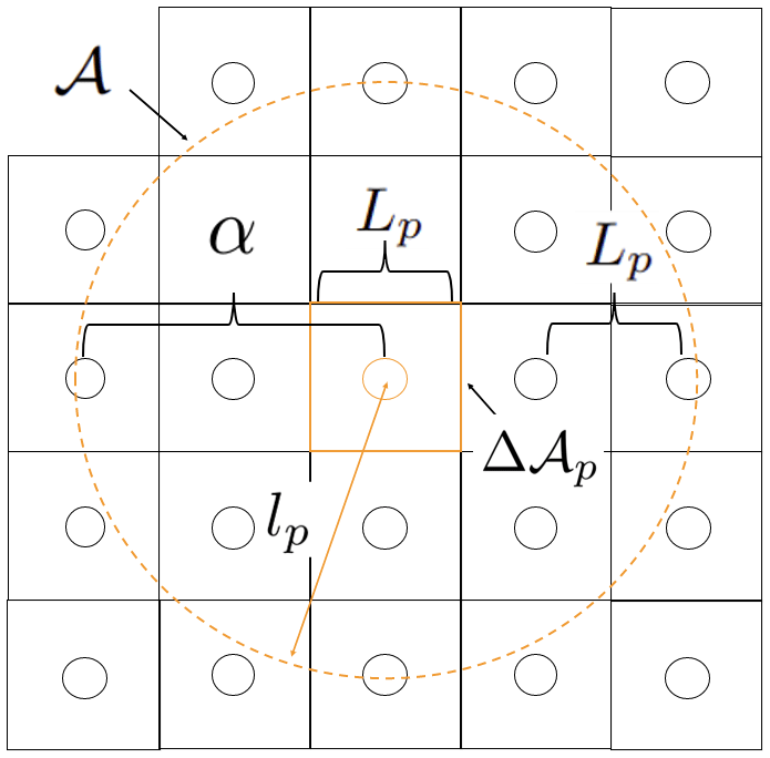
Figure 1 Graphical representation of the initial position of the particles and the relevant parameter for the smoothing length evolution: the ice area carried by the particle Δ𝒜_p (solid orange square), the parameter α (=2 in this schematic for visibility), the support domain 𝒜 (dashed orange line), the smoothing length l_p (red arrow) and the initial distance between particles L_p. Black circles are neighbouring particles q, and the orange circle is the current particle p. Note that, as for Fig. A1, the particle sizes in this schematic are also arbitrary.

The smoothing length l_p is capped to 10 times its initial value when the particle density tends to zero. This capping prevents conservation of mass for a density lower than 1 % of its initial value (see Eq. 26). We justify this capping because such small densities do not affect the ice dynamics.

2.7 Boundary treatment

We implemented the boundary treatment of Monaghan and Kajtar (2009) because of its simplicity, versatility and low computational cost. The boundaries are set up by placing stationary particles with fixed smoothing length l_b and a mass m_b equal to the average ice particle mass m_p. The boundary smoothing length l_b is chosen in a way that only one layer of ice particles initially interact with the boundary (this makes l_b resolution-dependent). The boundary particles are (equally) spaced apart by a factor of 1/4 of their smoothing length ($l_{\mathrm{b}}/\mathrm{4}$). In this manner, all ice particles p within a support domain l_b will interact with approximately four boundary particles (denoted by the subscript b) at a time, resulting in a net normal repulsive force ${{\mathit{F}}_{\mathit{N}}}_{\mathrm{p}}$,

$$\begin{array}{}\text{(28)}& {{\mathit{F}}_{\mathit{N}}}_{\mathrm{p}}=\sum _{b=\mathrm{1}}^{N_b}\mathit{\mu }{\displaystyle \frac{({\mathit{r}}_{\mathrm{p}}-{\mathit{r}}_b)}{|{\mathit{r}}_{\mathrm{p}}-{\mathit{r}}_b{|}^{\mathrm{2}}}}{W}_{pb}{\displaystyle \frac{\mathrm{2}{m}_{\mathrm{b}}}{m_{\mathrm{p}}+m_{\mathrm{b}}}},\end{array}$$

which is added to their momentum equation. In Eq. (28), μ is a constant with units of kg m⁴ s⁻² used to adjust the repulsion strength and is also simulation-dependent because it needs to counterbalance the particle acceleration and prevent them from escaping the domain. This free parameter is not suited for complex pan-arctic simulations but is sufficient in our idealized experiments. For all the simulations, a free-slip boundary condition, i.e., no tangential friction force between boundary particle and ice particle, is applied.

Table 1 Physical parameters used in ridging and arch simulations.

Values of the parameters used for the simulations are the same as the ones presented in Williams et al. (2017) to facilitate comparison in the Results section.

3 Results

3.1 Plastic wave propagation

We first compare the plastic wave speed for the VP dynamic equations with and without the SPH approximations. To this end, we do a perturbation analysis for a 1D case with a fixed sea-ice concentration (A=1). In this case, the 1D SPH sea-ice dynamic equations (Eqs. 13–16) form a system of three equations and three unknowns (x, u and h):

$$\begin{array}{}\text{(29)}& {\displaystyle \frac{\text{D}{x}_{\mathrm{p}}}{\text{D}t}}=u_{\mathrm{p}},\text{(30)}& {\displaystyle \frac{\text{D}{u}_{\mathrm{p}}}{\text{D}t}}=\mathrm{\Gamma }\sum _{q=\mathrm{1}}^N{\displaystyle \frac{m_{\mathrm{q}}}{{\mathit{\rho }}_{\mathrm{i}}^{\mathrm{2}}}}({\displaystyle \frac{\mathrm{1}}{h_{\mathrm{q}}}}+{\displaystyle \frac{\mathrm{1}}{h_{\mathrm{p}}}}){\displaystyle \frac{x_{\mathrm{pq}}}{\left|x_{\mathrm{pq}}\right|}}{\displaystyle \frac{\partial W}{\partial x_{\mathrm{pq}}}}+{\mathit{\tau }}_{\mathrm{p}},\text{(31)}& {\displaystyle \frac{\text{D}{h}_{\mathrm{p}}}{\text{D}t}}=-{\displaystyle \frac{\mathrm{1}}{{\mathit{\rho }}_{\mathrm{i}}}}\sum _{q=\mathrm{1}}^N{m}_{\mathrm{q}}(u_{\mathrm{q}}-u_{\mathrm{p}}){\displaystyle \frac{x_{\mathrm{pq}}}{\left|x_{\mathrm{pq}}\right|}}{\displaystyle \frac{\partial W}{\partial x_{\mathrm{pq}}}},\end{array}$$

where x_pq is a short form for x_p−x_q and

$$\begin{array}{}\text{(32)}& \mathrm{\Gamma }={\displaystyle \frac{P^{*}}{\mathrm{2}}}[\pm (e^{-\mathrm{2}}+\mathrm{1}{)}^{\mathrm{1}/\mathrm{2}}-\mathrm{1}].\end{array}$$

In the above, we made use of the following 1D normal stress for convergent plastic motion (see Gray, 1999; Williams et al., 2017, for 1D normal stress derivation):

$$\begin{array}{}\text{(33)}& \mathit{\sigma }={\mathit{\sigma }}_{xx}={\displaystyle \frac{P^{*}}{\mathrm{2}}}[\pm (e^{-\mathrm{2}}+\mathrm{1}{)}^{\mathrm{1}/\mathrm{2}}-\mathrm{1}]h=\mathrm{\Gamma }h.\end{array}$$

Linearizing around a mean state ($\stackrel{\mathrm{‾}}{u}=\mathrm{0}$ and $\stackrel{\mathrm{‾}}{h}=h_{\mathrm{0}}$), considering small perturbations (δx, δu and δh) and ignoring the second-order term, we obtain

$$\begin{array}{}\text{(34)}& {\displaystyle \frac{\text{D}\mathit{\delta }{x}_{\mathrm{p}}}{\text{D}t}}=\mathit{\delta }{u}_{\mathrm{p}},\text{(35)}& {\displaystyle }\begin{array}{rl}{\displaystyle \frac{\text{D}\mathit{\delta }{u}_{\mathrm{p}}}{\text{D}t}}& ={\displaystyle \frac{\mathrm{\Gamma }}{{\mathit{\rho }}_{\mathrm{i}}}}\sum _{q=\mathrm{1}}^N\mathrm{\Delta }{\mathcal{A}}_{\mathrm{q}}{\displaystyle \frac{{\stackrel{\mathrm{‾}}{x}}_{\mathrm{pq}}}{\left|{\stackrel{\mathrm{‾}}{x}}_{\mathrm{pq}}\right|}}\left({\displaystyle \frac{-\mathrm{1}}{h_{\mathrm{0}}}}\right(\mathit{\delta }{h}_{\mathrm{q}}+\mathit{\delta }{h}_{\mathrm{p}}){\displaystyle \frac{\partial W}{\partial {\stackrel{\mathrm{‾}}{x}}_{\mathrm{pq}}}}\\ & +\mathrm{2}(\mathit{\delta }{x}_{\mathrm{p}}-\mathit{\delta }{x}_{\mathrm{q}}){\displaystyle \frac{{\partial }^{\mathrm{2}}W}{\partial {\stackrel{\mathrm{‾}}{x}}_{\mathrm{pq}}^{\mathrm{2}}}}),\end{array}\text{(36)}& {\displaystyle \frac{\text{D}\mathit{\delta }{h}_{\mathrm{p}}}{\text{D}t}}=-h_{\mathrm{0}}\sum _{q=\mathrm{1}}^N\mathrm{\Delta }{\mathcal{A}}_{\mathrm{q}}{\displaystyle \frac{{\stackrel{\mathrm{‾}}{x}}_{\mathrm{pq}}}{\left|{\stackrel{\mathrm{‾}}{x}}_{\mathrm{pq}}\right|}}(\mathit{\delta }{u}_{\mathrm{q}}-\mathit{\delta }{u}_{\mathrm{p}}){\displaystyle \frac{\partial W}{\partial {\stackrel{\mathrm{‾}}{x}}_{\mathrm{pq}}}},\end{array}$$

where $\mathrm{\Delta }{\mathcal{A}}_{\mathrm{q}}=\frac{m_{\mathrm{q}}}{{\mathit{\rho }}_{\mathrm{i}}{h}_{\mathrm{0}}}=\frac{m_{\mathrm{q}}}{{\mathit{\rho }}_{\mathrm{q}}}$ (Eq. A4) and where we have used the binomial expansion $\frac{\mathrm{1}}{h}=\frac{\mathrm{1}}{h_{\mathrm{0}}+\mathit{\delta }h}\approx \frac{\mathrm{1}}{h_{\mathrm{0}}}(\mathrm{1}-\frac{\mathit{\delta }h}{h_{\mathrm{0}}})$. Following Williams et al. (2017), we do a perturbation analysis on the system of Eqs. (34)–(36) and assume a wave solution of the form $\mathit{\delta }f=\widehat{f}\text{exp}\left(i\right(k\stackrel{\mathrm{‾}}{x}-\mathit{\omega }t\left)\right)$, where i is the imaginary number; k is the wavenumber; ω is the angular velocity; and f is a dummy variable standing for u, x and h. Substituting δf in Eqs. (34)–(36), the resulting set of equations in the reference frame following the ice motion reduces to

$$\begin{array}{}\text{(37)}& {\displaystyle }\widehat{x}={\displaystyle \frac{i}{\mathit{\omega }}}\widehat{u},\text{(38)}& {\displaystyle }\begin{array}{rl}\widehat{u}& ={\displaystyle \frac{i\mathrm{\Gamma }}{\mathit{\omega }{\mathit{\rho }}_{\mathrm{i}}}}\sum _{q=\mathrm{1}}^N{\mathcal{A}}_{\mathrm{q}}{\displaystyle \frac{{\stackrel{\mathrm{‾}}{x}}_{\mathrm{pq}}}{\left|{\stackrel{\mathrm{‾}}{x}}_{\mathrm{pq}}\right|}}\left(\right[-{\displaystyle \frac{\widehat{h}}{h_{\mathrm{0}}}}(\mathrm{1}+\text{exp}(-ik{\stackrel{\mathrm{‾}}{x}}_{\mathrm{pq}}\left)\right)]{\displaystyle \frac{\partial W}{\partial {\stackrel{\mathrm{‾}}{x}}_{\mathrm{pq}}}}\\ & +\mathrm{2}\widehat{x}(\mathrm{1}-\text{exp}(-ik{\stackrel{\mathrm{‾}}{x}}_{\mathrm{pq}}\left)\right){\displaystyle \frac{{\partial }^{\mathrm{2}}{W}_{\mathrm{pq}}}{\partial {\stackrel{\mathrm{‾}}{x}}_{\mathrm{pq}}^{\mathrm{2}}}}),\end{array}\text{(39)}& {\displaystyle }\widehat{h}=-{\displaystyle \frac{i{h}_{\mathrm{0}}\widehat{u}}{\mathit{\omega }}}\sum _{q=\mathrm{1}}^N{\mathcal{A}}_{\mathrm{q}}{\displaystyle \frac{{\stackrel{\mathrm{‾}}{x}}_{\mathrm{pq}}}{\left|{\stackrel{\mathrm{‾}}{x}}_{\mathrm{pq}}\right|}}\left(\text{exp}\right(-ik{\stackrel{\mathrm{‾}}{x}}_{\mathrm{pq}})-\mathrm{1}).\end{array}$$

Note that since the ice is initially at rest, the Lagrangian and the Eulerian frameworks are equivalent. For a large enough wavelength (so that the perturbation can be resolved across multiple particles with high accuracy, i.e., λ≥l_p and N→∞), the summations can be approximated by integrals over the space; i.e., ${\sum }_{q=\mathrm{1}}^N{\mathcal{A}}_{\mathrm{q}}\frac{{\stackrel{\mathrm{‾}}{x}}_{\mathrm{pq}}}{\left|{\stackrel{\mathrm{‾}}{x}}_{\mathrm{pq}}\right|}$ becomes ${\int }_{-\mathrm{\infty }}^{\mathrm{\infty }}\text{d}{\stackrel{\mathrm{‾}}{x}}_{\mathrm{pq}}$. Taking advantage of the kernel properties – i.e., all moments higher than 0 vanish – we can write Eqs. (38)–(39) as

$$\begin{array}{}\text{(40)}& {\displaystyle }\begin{array}{rl}\widehat{u}& ={\displaystyle \frac{-i\mathrm{\Gamma }}{\mathit{\omega }{\mathit{\rho }}_{\mathrm{i}}}}\underset{-\mathrm{\infty }}{\overset{\mathrm{\infty }}{\int }}({\displaystyle \frac{\widehat{h}}{h_{\mathrm{0}}}}{\displaystyle \frac{\partial W}{\partial {\stackrel{\mathrm{‾}}{x}}_{\mathrm{pq}}}}+\mathrm{2}\widehat{x}{\displaystyle \frac{{\partial }^{\mathrm{2}}{W}_{\mathrm{pq}}}{\partial {\stackrel{\mathrm{‾}}{x}}_{\mathrm{pq}}^{\mathrm{2}}}})\text{exp}(-ik{\stackrel{\mathrm{‾}}{x}}_{\mathrm{pq}})\text{d}{\stackrel{\mathrm{‾}}{x}}_{\mathrm{pq}}\\ & ={\displaystyle \frac{\mathrm{\Gamma }}{\mathit{\omega }{\mathit{\rho }}_{\mathrm{i}}}}({\displaystyle \frac{\widehat{h}}{h_{\mathrm{0}}}}k+i\mathrm{2}{k}^{\mathrm{2}}\widehat{x})\stackrel{\mathrm{̃}}{W},\end{array}\text{(41)}& {\displaystyle }\widehat{h}=-{\displaystyle \frac{i{h}_{\mathrm{0}}\widehat{u}}{\mathit{\omega }}}\underset{-\mathrm{\infty }}{\overset{\mathrm{\infty }}{\int }}\text{exp}(-ik{\stackrel{\mathrm{‾}}{x}}_{\mathrm{pq}}){\displaystyle \frac{\partial W}{\partial {\stackrel{\mathrm{‾}}{x}}_{\mathrm{pq}}}}\text{d}{\stackrel{\mathrm{‾}}{x}}_{\mathrm{pq}}={\displaystyle \frac{h_{\mathrm{0}}\widehat{u}k}{\mathit{\omega }}}\stackrel{\mathrm{̃}}{W},\end{array}$$

where the integrals have been converted to Fourier transform using $\mathcal{F}\left(\frac{\partial W}{\partial {\stackrel{\mathrm{‾}}{x}}_{\mathrm{pq}}}\right)={\int }_{-\mathrm{\infty }}^{\mathrm{\infty }}\left(\frac{\partial W}{\partial {\stackrel{\mathrm{‾}}{x}}_{\mathrm{pq}}}\right)\text{exp}(-ik{\stackrel{\mathrm{‾}}{x}}_{\mathrm{pq}})\text{d}{\stackrel{\mathrm{‾}}{x}}_{\mathrm{pq}}=ik\mathcal{F}\left(W\right)=ik\stackrel{\mathrm{̃}}{W}$. Finally, Eqs. (37), (40) and (41) represent a system of three equations for three unknowns ($\widehat{x}$, $\widehat{u}$, $\widehat{h}$) that we solve by substitution. This leads to the following form for the phase speed of the plastic wave ($\frac{\mathit{\omega }}{k}$):

$$\begin{array}{}\text{(42)}& c_{\text{SPH}}={\displaystyle \frac{\mathit{\omega }}{k}}=\pm \stackrel{\mathrm{̃}}{W}\sqrt{-{\displaystyle \frac{\mathrm{\Gamma }}{{\mathit{\rho }}_{\mathrm{i}}}}({\displaystyle \frac{\mathrm{2}}{\stackrel{\mathrm{̃}}{W}}}-\mathrm{1})}.\end{array}$$

For wavelengths much larger than the smoothing length ($\mathit{\lambda }\propto \frac{\mathrm{1}}{k}\gg l_{\mathrm{p}}$), the Fourier transform of the kernel tends to 1 ($\stackrel{\mathrm{̃}}{W}\approx \mathrm{1}$) and the SPH formulation reduces to the viscous–plastic theory without SPH approximations (see for instance Williams et al., 2017), i.e.,

$$\begin{array}{}\text{(43)}& c_{\text{VP}}=\pm \sqrt{-{\displaystyle \frac{\mathrm{\Gamma }}{{\mathit{\rho }}_{\mathrm{i}}}}},\end{array}$$

with a plastic wave propagation speed c_VP≈5.7 m s⁻¹ for typical sea-ice parameters (see Table 1). Consequently, a major difference of SPH with the FDM framework is that the plastic wave speed is dispersive with a phase velocity c_SPH that is dependent on the wavelength and the smoothing length. In general, only the plastic waves with a wavelength between approximately 1 and 11 times the smoothing length will have their travelling speed modified by more than 1 %. More specifically, in the limit where the wavelength λ approaches the smoothing length l_p, the plastic wave speed increases in the SPH framework to a maximum value of ≈6.7 m s⁻¹ (see Fig. 2a). Note that for wavelengths smaller than the smoothing length, the summations in Eqs. (40)–(41) cannot be written as integrals, but the particles still respond partially to the perturbations. This sometimes leads to the tensile and the zero-energy mode instabilities (Swegle et al., 1995). As mentioned above, Dehnen and Aly (2012) showed that Wendland kernels can diminish the tensile instability and the pairing of particles. A deeper analysis of unresolved waves (λ<l_p) in the context of sea-ice SPH dynamic equations is beyond the scope of the current study.

For the more general case when the base state allows for a variable concentration (linearized around a mean state $\stackrel{\mathrm{‾}}{A}=A_{\mathrm{0}}$) and considering the classical – denoted by a superscript C – particle density definition (${\mathit{\rho }}_{\mathrm{p}}^{\text{C}}={\mathit{\rho }}_{\mathrm{i}}{h}_{\mathrm{p}}{A}_{\mathrm{p}}$) used by Wang et al. (1998), Ji et al. (2005), and Staroszczyk (2017), the plastic wave speed becomes

$$\begin{array}{}\text{(44)}& c_{\text{A,SPH}}^{\text{C}}=\pm \stackrel{\mathrm{̃}}{W}\sqrt{-{\displaystyle \frac{{\mathrm{\Gamma }}^{*}}{{\mathit{\rho }}_{\mathrm{i}}}}(C{A}_{\mathrm{0}}-\mathrm{3}+{\displaystyle \frac{\mathrm{2}}{\stackrel{\mathrm{̃}}{W}}})},\end{array}$$

where ${\mathrm{\Gamma }}^{*}=\mathrm{\Gamma }\text{exp}(-C(\mathrm{1}-A_{\mathrm{0}}\left)\right)$. We argue that the plastic wave speed $c_{\text{A,SPH}}^{\text{C}}$ obtained with the classical density definition does not converge (see Fig. 2b) to the viscous–plastic theory, c_A,VP, derived from FDM (see Williams et al., 2017, for a derivation),

$$\begin{array}{}\text{(45)}& c_{\text{A,VP}}=\pm \sqrt{-{\displaystyle \frac{{\mathrm{\Gamma }}^{*}}{{\mathit{\rho }}_{\mathrm{i}}}}(C{A}_{\mathrm{0}}+\mathrm{1})},\end{array}$$

because the ice concentration is taken into account in both the definition of ${\mathit{\rho }}_{\mathrm{p}}^{\text{C}}$ and implicitly in the definition of the average thickness h_p. When we consider the new formulation of particle density independent of concentration as proposed above (Eq. 18), the wave speed equation becomes

$$\begin{array}{}\text{(46)}& c_{\text{A,SPH}}=\pm \stackrel{\mathrm{̃}}{W}\sqrt{-{\displaystyle \frac{{\mathrm{\Gamma }}^{*}}{{\mathit{\rho }}_{\mathrm{i}}}}(C{A}_{\mathrm{0}}-\mathrm{1}+{\displaystyle \frac{\mathrm{2}}{\stackrel{\mathrm{̃}}{W}}})},\end{array}$$

which reduces to the FDM VP theory (Eq. 45) when the wavelength is large compared to the smoothing length (see Fig. 2c). Note that the perturbation analysis presented above is not valid for the classical density definition proposed by Wang et al. (1998), Ji et al. (2005), and Staroszczyk (2017) since they use a different set of momentum, continuity and constitutive equations to describe sea ice. In a similar manner to the plastic wave speed with a fixed concentration (Eq. 42), the wave speed c_A,SPH (Eq. 46) is dispersive and the wavelengths between 1 and 11 times the smoothing length are those that are mostly affected (more than 1 %). However, in this case, the plastic wave speed is damped for wavelengths close to the smoothing length for a mean concentration state higher than 0.1. Note that while the plastic wave speed is defined for all A, it does not have a physical meaning for A<0.85 since there are negligible ice–ice interactions.

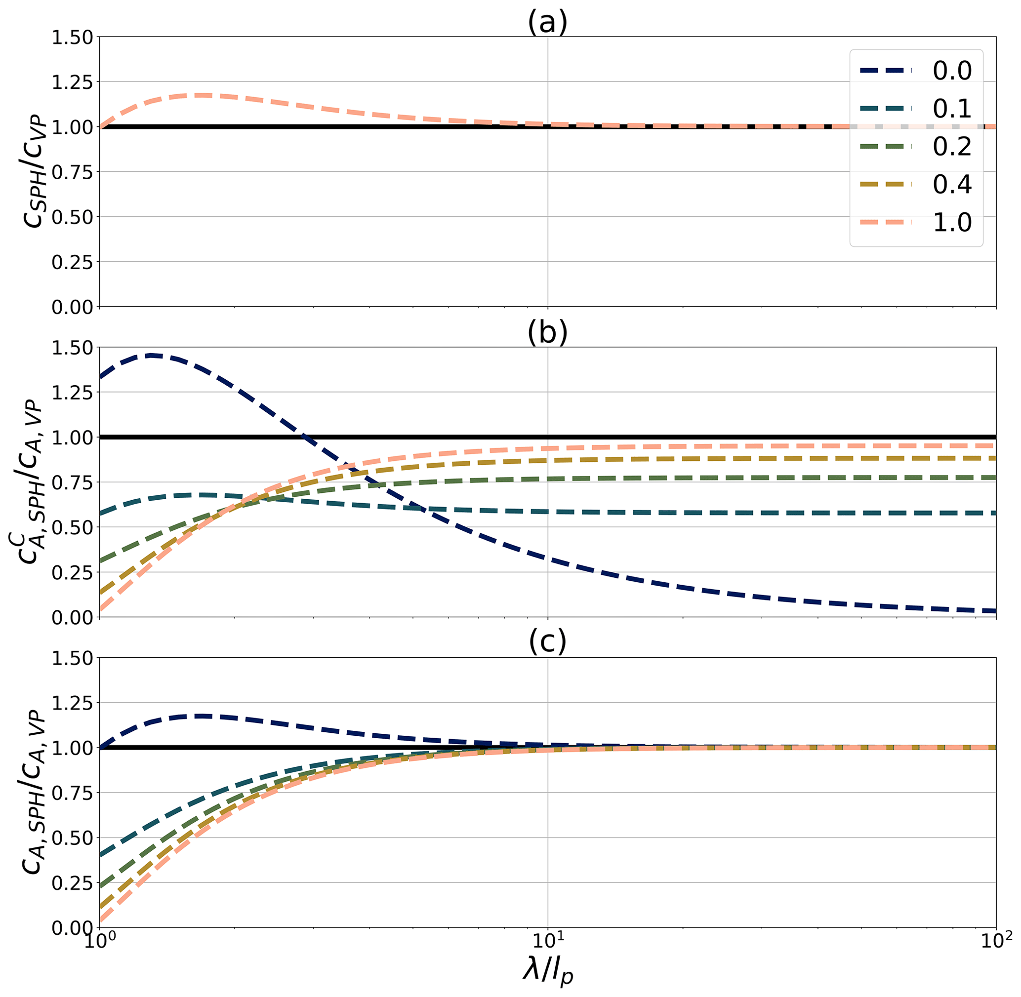
Figure 2 SPH plastic wave speed as a function of the normalized wavelength ($\mathit{\lambda }/l_{\mathrm{p}}$) for the Wendland C⁶ kernel. Panel (a) shows the classical VP rheology with fixed concentration (Eq. 42) normalized by the FDM plastic wave speed with fixed concentration (Eq. 43), (b) shows the classical VP rheology with a variable concentration and the density definition ${\mathit{\rho }}_{\mathrm{p}}^{\text{C}}={\mathit{\rho }}_{\mathrm{i}}{h}_{\mathrm{p}}{A}_{\mathrm{p}}$ (Eq. 44) normalized by the FDM plastic wave speed with a variable concentration (Eq. 45), and (c) shows the classical VP rheology with a variable concentration and the density definition ρ_p=ρ_ih_p (Eq. 46) normalized by the FDM plastic wave speed with a variable concentration (Eq. 45). Different homogeneous base states of concentration A₀ are shown varying from 0 to 1.

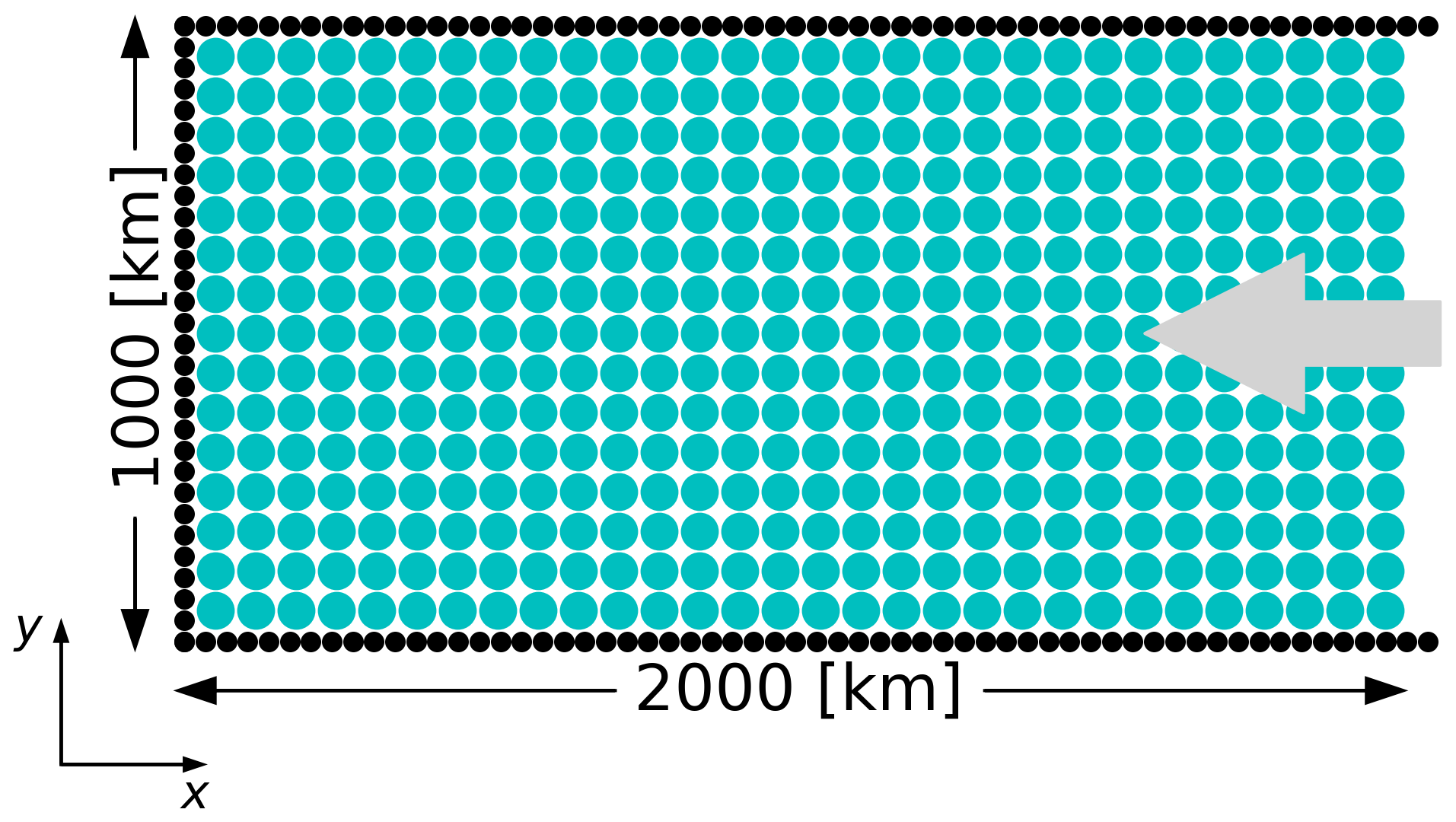
Figure 3 Idealized domain of the ridging experiment. The blue circles represent the ice particles, and the black ones are the boundary particles. The grey arrow shows the wind forcing. More particles than shown in this schematic were used during the simulation.

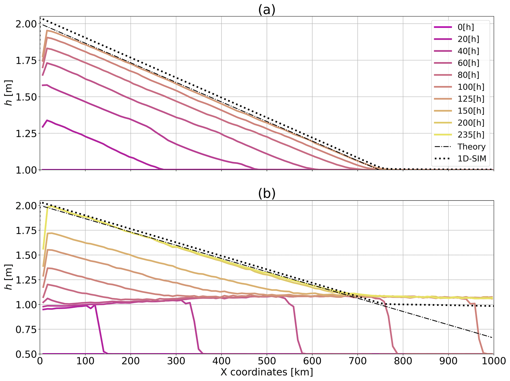
Figure 4 Temporal evolution of simulated sea-ice thickness along the central horizontal line of the domain for (a) the ridge experiment initialized with a concentration A=1 and average thickness h=1 m and (b) the ridge experiment initialized with a concentration A=0.5 and average thickness h=0.5 m. The wall is located at x=0, and the wind speed is $-\mathrm{5}\widehat{\mathit{x}}$ m s⁻¹. The theory follows Eq. (47).

3.2 Ridging experiments

We validate our implementation of the SPH model (with the new definition of particle density ρ_p) in a 1D ridging experiment for which we can validate against the simulated field from a viscous–plastic sea-ice model based on the FDM – the 1D version of McGill-SIM model used in the SIREx studies (Bouchat et al., 2022; Hutter et al., 2022) – and against the analytical solution (see Williams and Tremblay, 2018, for a derivation):

$$\begin{array}{}\text{(47)}& -{\displaystyle \frac{\text{d}\mathit{\sigma }}{\text{d}x}}={\mathit{\rho }}_a{C}_a\left|u_a\right|u_a\Rightarrow {\displaystyle \frac{\text{d}h}{\text{d}x}}={\displaystyle \frac{\mathrm{2}{\mathit{\rho }}_a{C}_a\left|u_a\right|u_a}{P^{*}(\sqrt{e^{-\mathrm{2}}+\mathrm{1}}+\mathrm{1})}},\end{array}$$

i.e., a linear profile in thickness with a slope proportional to the square of the wind velocity and inversely proportional to the ice strength. We consider a rectangular domain of 1000 by 2000 km including the boundary (the ice field is 1900 km to ensure that no particles escape on the open side) with 37 240 particles; an initial homogeneous smoothing length l_p of 21.429 km (spacing $l_{\mathrm{p}}/\mathit{\alpha }=\mathrm{7.14}$ km); and a smaller – to limit boundary effect – boundary particle smoothing length l_b of 4 km (spacing $l_{\mathrm{b}}/\mathrm{4}=\mathrm{1.0}$ km) to represent the wall (see Fig. 3). Particles are initialized with an average thickness h=1 m and a concentration A=1. They are forced against the wall by a constant unidirectional wind of 5 m s⁻¹. Note that the water stress is removed in the simulation for a faster convergence to the steady state, which enables higher resolution – a water current of 0 m s⁻¹ would slow down the ice and the ridge formation since it is driven by the advection speed. The Coriolis force should normally also have to be considered with this domain size at classical polar latitude – the Rossby number is 𝒪(10⁻²) – but is neglected in this idealized experiment to conserve the symmetry of the solution and compare it to the theoretical 1D equation (Eq. 47). In results presented below (Figs. 4–5), the particle properties are averaged over a grid of approximately 10 by 5 km cells for plotting purposes.

Results show that the simulated thickness field converges to the analytical solution (within an error of ≈1 %) after ≈5 d with a slope of $\mathrm{1.33}\times {\mathrm{10}}^{-\mathrm{3}}$ m km⁻¹, compared to $\mathrm{1.34}\times {\mathrm{10}}^{-\mathrm{3}}$ m km⁻¹ for the theory – lower-resolution simulations were run for a longer time and also converged to this stable state (results not shown). This is comparable to the precision obtained by the 1D McGill-SIM FDM model which reaches a slope of $\mathrm{1.35}\times {\mathrm{10}}^{-\mathrm{3}}$ m km⁻¹. Artifacts are observed close to the boundary where the repulsive force prevents the particles from reaching the “wall”. Additionally, when a particle comes into contact with the boundary with a certain inertia (due to the $\mathrm{1}/\mathit{r}$ dependence of the boundary force), we observe oscillations in the motion of particles which can propagate far in the domain (e.g., Fig. 4a, at $x\approx [\mathrm{50},\mathrm{300}]$ km and $t=[\mathrm{30},\mathrm{45}]$ h). The oscillations are damped, and the energy is dissipated by the rheology term with time until an equilibrium is reached. Note that reintroducing the water drag diminishes the oscillation coming from the boundary but does not remove them completely. A more physical boundary treatment is beyond the scope of this study.

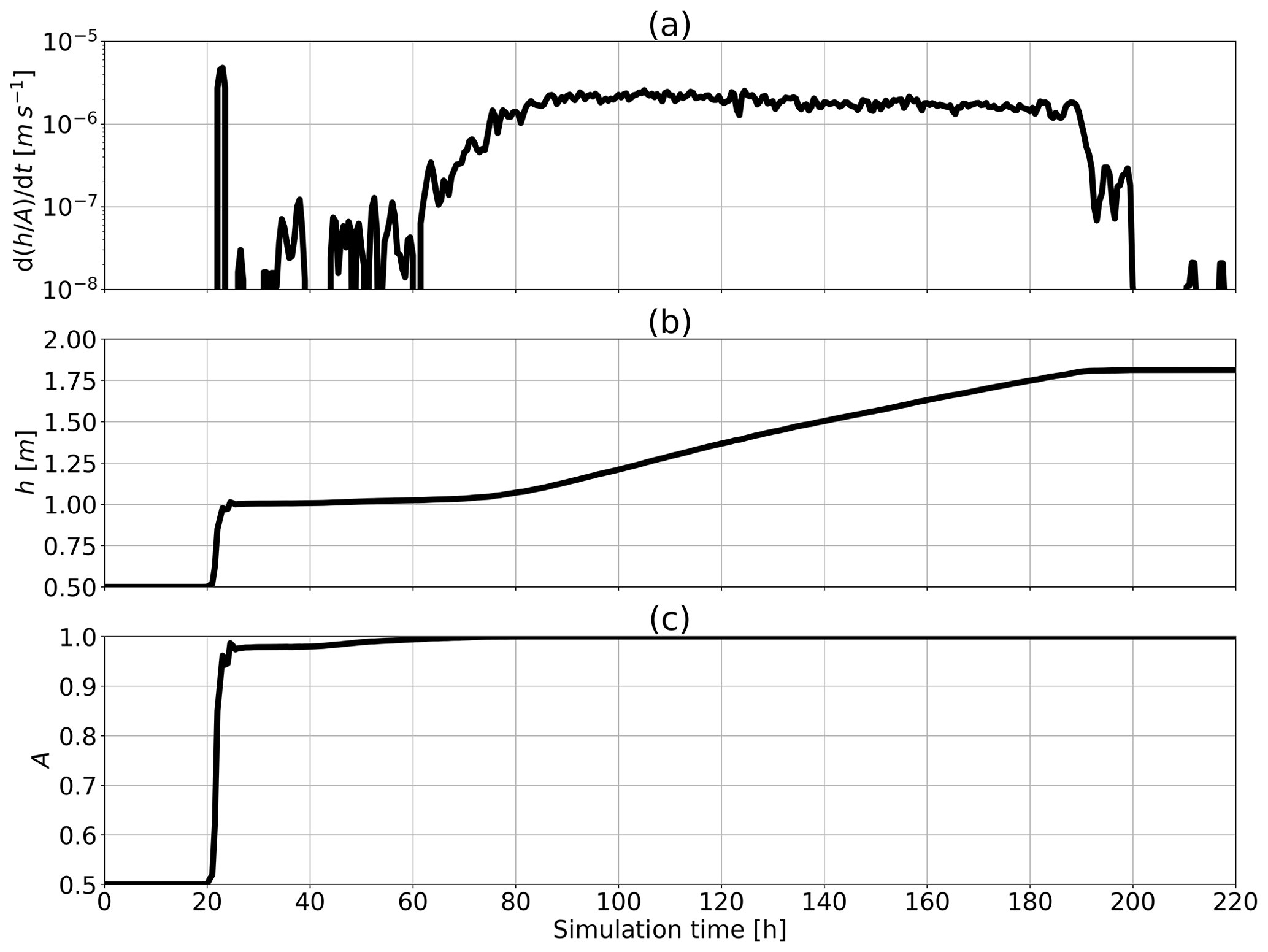
Figure 5 Evolution in time of (a) the thickness normalized by concentration rate of change in time $\frac{\text{d}(h/A)}{\text{d}t}$, (b) the average thickness h and (c) the concentration A at x=300 km. The rate of change in time is computed from $\frac{\text{d}f}{\text{d}t}(x,t)=\frac{f(x,t+\mathrm{\Delta }t)-f(x,t-\mathrm{\Delta }t)}{\mathrm{2}\mathrm{\Delta }t}$.

We also repeated the ridge experiment with the same forcing and total sea-ice volume but letting the sea-ice concentration evolve with time. Specifically, the initial average thickness and concentration were set to h=0.5 m and A=0.5. This ensures that both h and A covary in time such that $\frac{h}{A}$ remains constant – note that A and h follow the same continuity Eqs. (15) and (16) or (4) and (5) when omitting the SPH approximations, and therefore they should vary identically in time until A reaches 1 – in the marginal ice zone (MIZ), which we define as the area where the sea-ice concentration ranges between 0.15 and 0.85 and where low ridging by ice collision occurs (see Fig. 4b). To accomplish this, the domain was extended to 4000 km (3800 km, excluding the boundaries) and the initial particles spacing changed from 7.14 km to 10.0 km for a corresponding initial smoothing length l_p of 30.0 km and total number of particles of 38 000. In this configuration, the model converges to a steady-state solution in ≈10 d with a slope of $\mathrm{1.36}\times {\mathrm{10}}^{-\mathrm{3}}$ m km⁻¹, in agreement with theory within an error of ≈1 % (see Fig. 4b). Results at x=300 km, away from boundary effects, show that (as desired) thickness and concentration evolve coherently – $\frac{\text{d}(h/A)}{\text{d}t}\approx \mathrm{0}$ – before ice concentration reaches ≈85 % (see Fig. 5a). At that point (t≈22 h), ice–ice interactions emerge and the ridging process starts $\left(\frac{\text{d}(h/A)}{\text{d}t}>\mathrm{0}\right)$. One key difference with the simulation initialized at A=1 is a thickness build-up (above 1 m) at the edge of the ridge in the MIZ. At this location, the continuity equation for sea-ice concentration is capped, while that of the mean ice thickness remains continuous. This results in a local increase in ice thickness to ≈1.1 m. This process is akin to the wave radiation drag in the MIZ (Sutherland and Dumont, 2018). A detailed analysis of simulations in simple convergent ice flow in the MIZ with ice concentration close to 100 % will be considered in future work.

In the ridge building phase, the speed of advance of the ridge front increases until a maximum concentration is reached after ≈70 h (see Fig. 5c). Subsequently, the ice drift speed reduces, and the rate of advance of the ridge slows down. When the ice thickness gradient is in balance with the surface wind stress (after ≈200 h), $\frac{\text{d}(h/A)}{\text{d}t}$ reaches a steady state. Overall, we can observe three stages in the ridge formation (see Fig. 5): first, a rapid compaction stage when ice particles are drifting close to their free-drift speed since the ice strength is weak; second, a transition stage between A≈0.85 and 1.00 when ridging occurs in the MIZ analogous to the wave radiation drag mentioned above; and third, a ridging stage with changes in ice thickness that are about 1 order of magnitude higher than during the transition stage. Note that the amplitude of oscillations between particles within the domain or at the boundaries in ridging experiments diminishes when incorporating the water drag (a damping term). The water drag also increases the time needed to reach steady state because the ice drift speed is slower.

3.3 Arch experiments

We next compare the SPH approach with the FDM and DEM sea-ice models in a second well-studied idealized experiment: the ice arch formation. To this end, we run the SPH model in an idealized domain representing the Nares Strait (see Fig. 6) with an upstream reservoir 5 times the length of the channel (L) to minimize the boundary confinement effect without sacrificing the spatial resolution.

The set of simulations uses a domain with L=60 km. The initial conditions for ice thickness, concentration and velocity are h=1 m, A=1 and u=0 m s⁻¹. The ice is forced with a constant unidirectional wind of −7.5 m s⁻¹ in the $\widehat{\mathit{y}}$ direction, and ocean current is fixed to u_w=0 m s⁻¹. The corresponding surface stress is ≈0.04 kN m⁻², and the total integrated stress at the entry of the channel is slightly smaller than P^* (${\int }_{\mathrm{0}}^{\mathrm{5}L}{\mathit{\tau }}_a\text{d}x=\mathrm{26.325}$ kN m⁻¹). We use a weaker wind than commonly used in Nares Strait ice arch simulations (≈10 m s⁻¹) to limit the ridging phase prior to the formation of the ice arch. In this experiment, we limit ourselves to ice with no tensile strength (k_t=0) and a shear strength of 6.875 kN m⁻², i.e., an ellipse aspect ratio of 2.

We suspect that the SPH and DEM frameworks have a similar behaviour in certain circumstances even though they have different (implicit) rheologies because of their Lagrangian nature. Indeed, the interpretation of the numerical representation of a particle in SPH as a collection of ice floes is also present in the DEM (Li et al., 2014), and the two numerical frameworks compute their quantities with one-to-one interactions. Consequently, we first test whether the SPH approach has the same sensitivity to the relative size of particles with respect to the channel width as in the DEM (Damsgaard et al., 2018). Results showed that no stable arch can be formed with the specified forcing for all particle diameter sizes tested (7.5, 5, 3.75 km) (see ice velocity field in Fig. 7). Instead, a “continuous” slow flow of ice is present in the channel. The discontinuity at the entry of the channel is visible in the concentration, thickness and velocity fields (Fig. 7) and can be interpreted as an intermittent (unstable) ice arch formation. Also, we noted that larger particles are not more prone to ice jam than smaller ones. This is contrary to what is known from granular material theory and to results from Damsgaard et al. (2018) that show a transition from stable to no ice arch formation for floe sizes ranging from approximately 1/4 to 1/16 of the strait's width. We explain this difference between SPH and DEM from the continuum description of the ice dynamics equation. In the present model, the constitutive laws prescribe the repulsion of the particles from one another according to the ice strength, which is a function dependent on the ice concentration and mean thickness, not on the particle size. We conclude that to enforce granularity within the SPH framework, the constitutive laws would need to be adapted to account for contact force and particle size which could then reproduce a similar behaviour to that observed in the DEM. However, even though the increase in resolution – or particle size – has no effect on the arch stability, it enables smaller fracture resolutions that are visible at the entrance of the channel (see ϵ_I and ϵ_II in Fig. 8). In our SPH model, the stress invariants σ_I and σ_II shows oscillation patterns in regions where the ice is in the viscous regime (see the tree-like structure in the normal and shear stress fields in Fig. 8). From our experiments, the “tree-like” peak stresses appear during the transient phase and at steady state. However, the particles never stop moving even in a steady state because viscous deformations are always present. We hypothesized that stress patterns are associated with over-damped elastic waves associated with small movements (but large internal stresses) of the particle in the viscous regime. Those structures are not symmetric, despite symmetrical initial conditions, because of the domino effect between interacting viscous waves. Note that they are absent from the strain-rate fields since viscous deformations are extremely small. They are also absent in sea-ice model based on a continuum approach (Dumont et al., 2009; Dansereau et al., 2017; Plante et al., 2020), but these tree-like structures are qualitatively similar to the stress structure between floes observed in the DEM (e.g., Damsgaard et al., 2018, Fig. 5c). Despite the fact that the model solves the same continuum equations as other FDM models, we believe that stress networks can be observed with the SPH method because particles interact in a pairwise fashion according to their relative distance. This can create less-dense ice areas within the medium which can lead to oscillations in the stress field. It is known that SPH can have spurious behaviour in some cases when the stress is solved at the same location as the particle centre (as done here). This can be avoided using stress particles (see Chalk et al., 2020, for details). More investigations are required to test whether this behaviour is physical. This is left for future work.

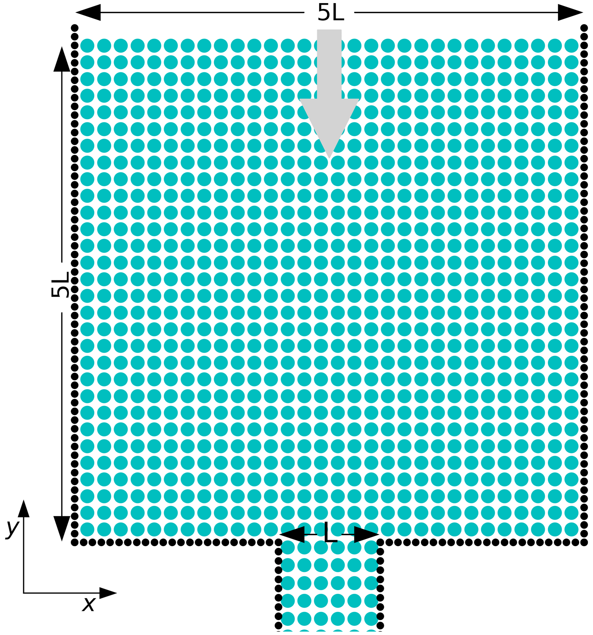
Figure 6 Idealized domain of the ice arch experiments. The blue circles represent the ice particles, and the black ones are the boundary particles. The grey arrow shows the wind forcing.

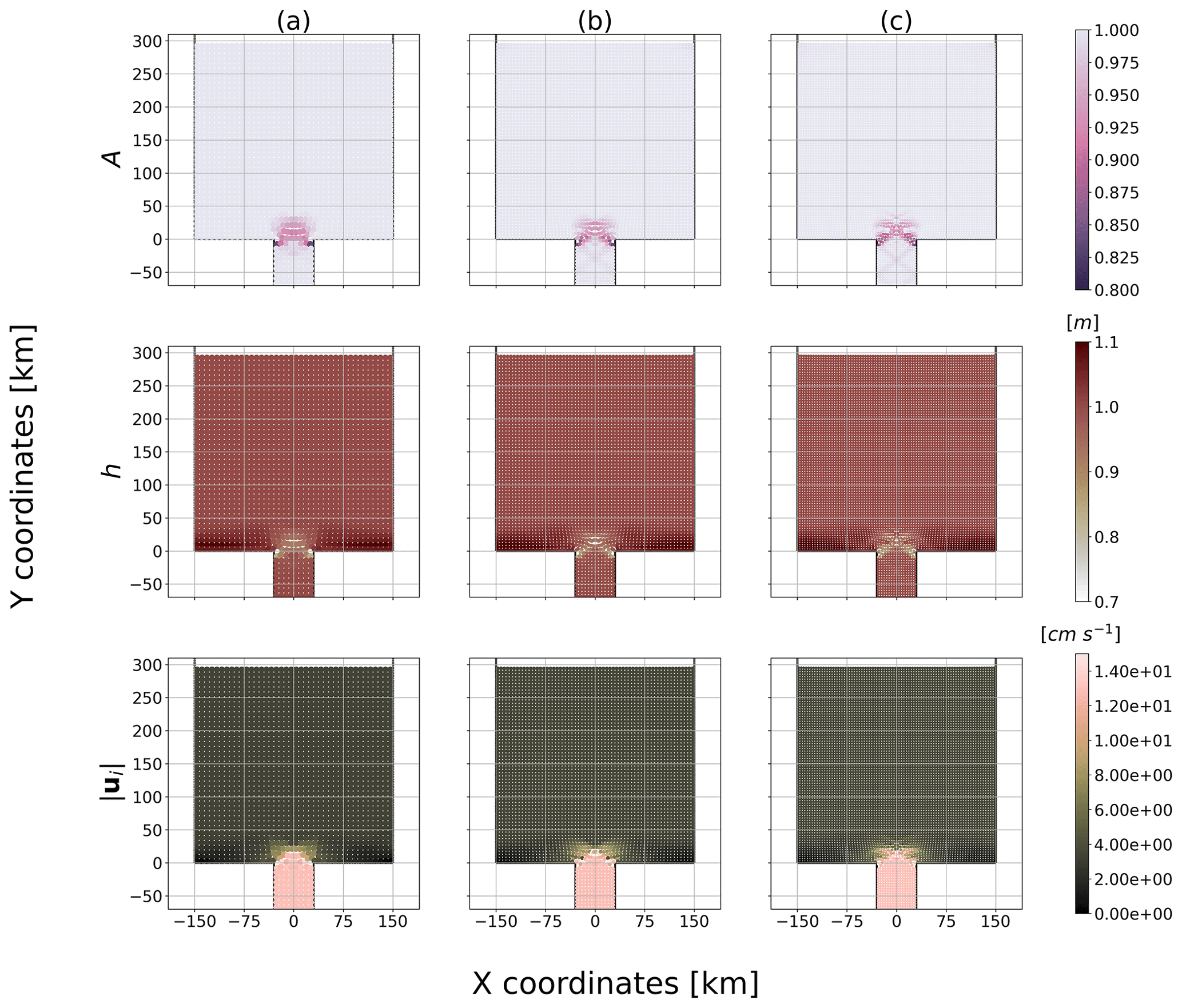
Figure 7 Ice concentration, thickness and total velocity (h, A, $\left|{\mathit{u}}_i\right|$) at time t=24 h for an initial particle spacing of (a) 7.5, (b) 5 and (c) 3.75 km (8, 12 and 16 particles can fit in the strait respectively), and the initial total integrated surface stress at the entry of the channel is 26.325 kN m⁻¹.

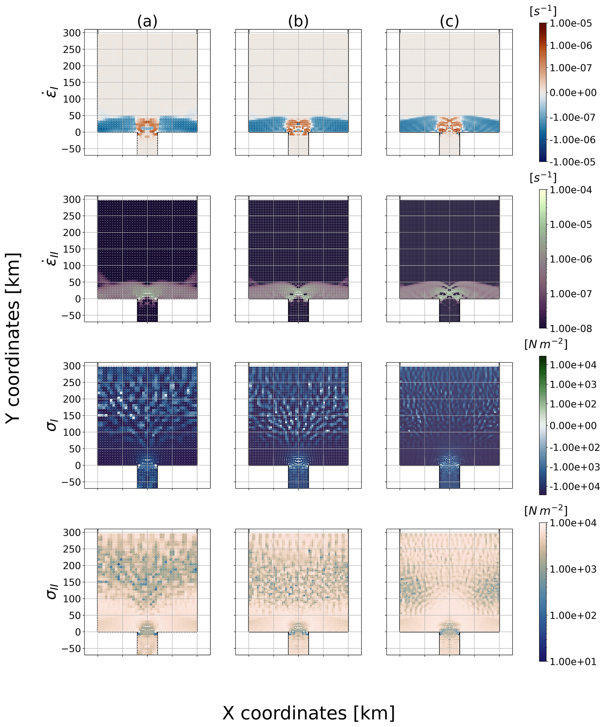
Figure 8 Strain rate and stress invariants (${\dot{\mathit{ϵ}}}_I$, ${\dot{\mathit{ϵ}}}_{II}$, σ_I, σ_II) at time t=24 h for an initial particle spacing of (a) 7.5, (b) 5 and (c) 3.75 km (8, 12 and 16 particles can fit in the strait respectively), and the initial total integrated surface stress at the entry of the channel is 26.325 kN m⁻¹.

Second, we explored the ability of the model to produce stable ice arches. To this end, we reduce the total integrated surface stress at the entry of the channel to 13.146 kN m⁻¹ (or wind speed of 5.3 m s⁻¹) to a value below the ice compressive strength (P^*) to avoid completely ridging the north of the channel and jump immediately to the arch-forming stage. In this case, the results show a clear stable arch (see Fig. 9) with a shape that is qualitatively similar to the one presented by Dansereau et al. (2017), Plante et al. (2020), and West et al. (2022). The formation of a stable arch in an SPH model is possible with the standard shear strength (e=2), in contrast to continuum models that require an increase in shear strength (e.g., Dumont et al., 2009; Dansereau et al., 2017; Plante et al., 2020) – it is important to keep in mind that the domain configurations were different in each of those studies. This suggests that SPH has a different sensitivity of ice arching to the ellipse aspect ratio e and ice thickness h. With a no-slip boundary condition and the same default yield curve (same P^* and ellipse aspect ratio e), preliminary results suggest that no arches form – the pack is undeformed – and instead a higher surface wind stress is required to form an arch. Note that in the SPH simulations, only one arch forms close to the outlet. Presumably, the number of arches would increase and location would change if the model was run at higher resolution, with different boundary conditions or in a non-idealized domain geometry. Overall, this shows that SPH is able to capture large-scale features coming from small-scale interactions. The simulation of a stable ice arch (Fig. 9) also shows how SPH can fracture and create discontinuities in the ice field as seen in DEM models. This behaviour is similar to that of the elastic-decohesive sea-ice constitutive model of Schreyer et al. (2006) or the FEM model of Rampal et al. (2016). Finally, in the SPH framework, a lead or polynya can be defined by an absence of particles for leads larger than particle size – akin to DEM – or by particles with reduced concentration for sub-particle size leads – akin to FDM.

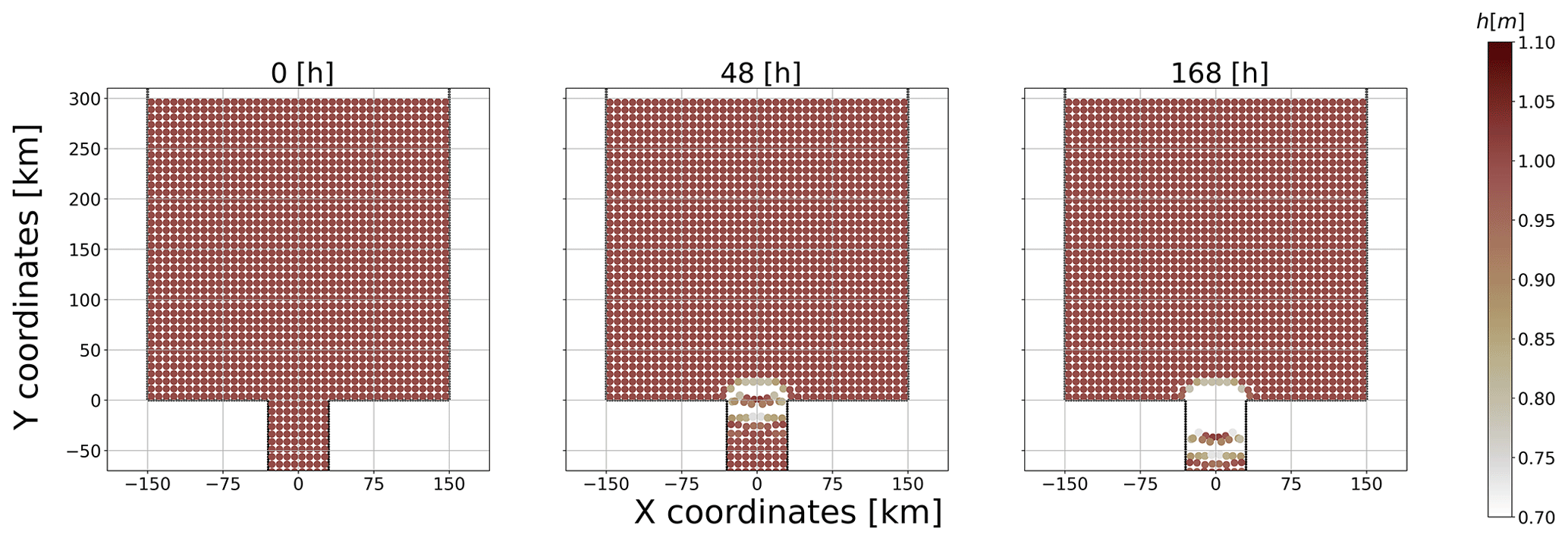
Figure 9 Thickness field at time t=0, 48 and 168 h for an initial particle spacing of 7.5 km and a total integrated stress at the entry of the channel of 13.146 kN m⁻¹.

4 Discussion and conclusion

In this paper, we have presented a first implementation of the viscous–plastic rheology with an elliptical yield curve and normal flow rule in the framework of SPH with the long-term goal of simulating synoptic-scale sea-ice dynamics. We have described the basics of the SPH approach and how the sea-ice dynamic equations can be formulated in this framework along with the implementation of key components of the numerical method such as the smoothing length, the kernel, the boundaries and the time integration technique. We proposed a different definition of the particle density and showed that the more commonly used density definition involving the ice concentration (Wang et al., 1998; Ji et al., 2005; Staroszczyk, 2017) when used together with the average ice thickness leads to erroneous plastic wave speed propagation. A particle density definition independent of the ice concentration corrects this and leads to results that are in line with the VP theory. The SPH model thus developed is in excellent agreement (error of ≈1 %) with an analytical solution of the VP ice dynamics for a simple 1D ridging experiment. The approximations used at the core of the SPH framework result in a dispersive plastic wave speed in the medium – in contrast to its FDM counterpart – which is dependent on the smoothing length (or resolution) and the choice of the kernel. The plastic wave speed is mostly affected for wavelengths 11 times the smoothing length and lower.

From the simple ridging experiment with fixed sea-ice concentration (A=1), we observe nonphysical damped oscillations that propagate in the domain associated with our choice of boundary conditions. The conclusions drawn from our simulations are robust to the choice of boundary conditions. Nevertheless, this behaviour needs to be removed for a proper simulation of sea ice near coastlines. The ridging experiment with an initial ice concentration below 100 % showed that continuity equations for concentration and thickness evolve coherently until a concentration of 85 %. At that point, SPH particles start to ridge locally in the MIZ in addition to the wall where the maximum stress is located. This effect is not observed in the continuum approach and is presumably related to particle collisions in converging motion.

When compared to other numerical frameworks, the SPH model is able to reproduce stable ice arches in an idealized domain of a strait with an ellipse aspect ratio of 2 and a wind forcing of 5.3 m s⁻¹, in contrast to other continuum approaches that require higher material shear strength. However, when using a stronger wind field of 7.5 m s⁻¹, no stable arches are formed when increasing the particles size in the strait (stable arches are only achieved when increasing particle average thickness). We concluded that the number of particles in the strait does not influence the formation of ice arches, in contrast to the DEM, and is analogous to an increase in resolution in a continuum framework: a larger number of particles influence the number of fractures that can form and the resolution of fine-scale structures. The stress fields produced by the SPH model in the channel experiment show a tree-like pattern upstream of the channel where there are low total deformations. This is not observed in FDM experiments, but it is qualitatively similar to the tensile stress network exhibited in DEM simulations (Damsgaard et al., 2018) that comes from individual contact force between the ice floes and is hypothesized to be associated with damped viscous sound waves.

Even though we successfully implemented the standard sea-ice viscous–plastic rheology with an elliptical yield curve and a normal flow rule in an SPH framework, the current model does not outperform a classical FDM model. In fact, there are inherent difficulties and instabilities in SPH that do not exist in FDM. It is known that the SPH framework trades consistency – i.e., the ability to correctly represent a differential equation in the limit of an infinite number of points with a null spacing between them – for stability, which gives the SPH a distinct feature of working well for many complicated problems with good efficiency but less accuracy. However, the classical formulation of SPH used and described in the present work does not usually respect zeroth-order consistency because of the unstructured particle position in space (see Belytschko et al., 1998, Sect. 3 for a derivation). Nevertheless, consistency can be improved at the expense of computational cost (Chen and Beraun, 2000; Liu et al., 2003) by reformulating the SPH core approximation (Eq. A1). Also, the boundary description has been identified as a weak point of the SPH framework. Prescribing Dirichlet, Neumann or Robin boundary conditions is not as straightforward as in continuum approaches. Moreover, preventing particle penetration through a boundary is still a challenging task (Liu and Liu, 2010), and the SPH consistency is usually at its worst at the boundary because the support domain is truncated. In the present study, a proper physical representation of the boundary was not adopted, and the boundary treatment was chosen for its numerical simplicity and should be modified in future work. Other major issues with SPH are the zero-energy modes and the tensile instability previously mentioned. The zero-energy modes can be found in FDM and FEM, and they correspond to modes at which the strain energy calculated is erroneously zero (Swegle et al., 1995). The tensile instability results in particle clumping or nonphysical fractures in the material. In the present work, we adopted a different kernel from the usual Gaussian spline to avoid those instabilities, but other methods such as the independent stress point (Dyka and Ingel, 1995; Chalk et al., 2020), artificial short-length repulsive force (Monaghan, 2000), particle repositioning (Sun et al., 2018) or adaptive kernel (Lahiri et al., 2020) can be used if more stabilization is needed. For example, at a smaller scale, SPH simulation of ice in uniaxial compression was improved by a simplified finite-difference interpolation scheme (Zhang et al., 2017). More specifically for sea-ice models, the pressure closure of Kreyscher et al. (2000) is not well-suited for long simulation. Indeed, particles can still move when they are in the viscous state but have low internal ice pressure because of the replacement pressure scheme. Consequently, particles could pass through each other resulting in erroneous locations of the parameters carried out. Finally, using SPH for sea-ice modules in grid-based continuum global climate models (GCMs) complicates the coupling with ocean and atmosphere components since particle quantities need to be converted on a grid and vice versa.

In its current state, the model reproduces very similar behaviour to other FDM continuum models and does not constitute a large improvement. Nevertheless, we believe that SPH enables the possibility to describe sea ice as a continuum at large scale using what is already known from continuum models and to explore some new avenues at small scales, where the continuity approximation is questionable. Indeed, SPH also has interesting properties that could be exploited. For example, SPH can be used with little change for problems involving several fluids, whether liquid, gas or dust fluids (Monaghan, 2012). This feature could be exploited in the creation of a general approach for all components of a GCM (atmosphere, ocean and sea ice). The method developed is also a proper option for nowcasting sea-ice prediction because only the ice dynamics need to be considered in nowcasting applications and the model has a good ability to carry the ice property in space. SPH can fracture and transition from the continuum to fragments seamlessly since it is not restricted on a grid, which also has the advantage of enabling ice edge shapes independent of it. The ability of SPH to move around particles has the interesting property of concentrating them in converging motion, effectively increasing the spatial resolution of the model in regions under high-stress activity and dispersing particles when the flow is divergent, which decreases the resolution in low-ice-concentration areas. This property should result in higher accuracy than that in typical continuum models. The elastic behaviour assumed for sea ice with a certain rheology can be associated with the weak compressibility inherent in the classical formulation of SPH. Finally, the SPH discretization of the continuum into particles enables the implementation of several new features. For example, angular momentum to individual floes (or pack of floes) can be added to take into account rotation along LKFs. A direct measure of the concentration from the number of particles within a support domain (this takes advantage of the already-computed number of neighbours and helps to ensure the desired number of neighbours in converging flow) can be computed. A subscale parametrization of floe–floe contact force (this short-length repulsive force could also help with the tensile instability) can be implemented. A varying floe size distribution could be incorporated by varying the mass carried by a particle for a given particle density.

For future work and before exploring new features enabled by the SPH numerical framework, a more physical treatment of the boundary conditions should be investigated to properly simulate the grounding of sea ice near the coast enabling the no-slip conditions. Subsequently, the model could be tested against other benchmark problems in an idealized domain to further understand and compare the effect of the SPH method (Flato, 1993; Hunke, 2001; Hibler et al., 2006; Danilov et al., 2015; Mehlmann et al., 2021). Also, in order to use the model for pan-Arctic simulations, the Coriolis and sea surface tilt force along with the treatment of the thermodynamics source and sink terms should be implemented in the SPH framework (see preliminary work by Staroszczyk, 2018). In addition, the parallelization of the code should be improved in order to bring the computational time down to a value comparable to that of an FDM model. Finally, while there still is a significant amount of work to be completed before SPH can be used in large-scale climate simulations, the method shows promise and deserves further investigations and development.

Appendix A: Smoothed particle hydrodynamics basics

The SPH method is at the interface between the finite-element and discrete-element methods. In this framework any function f(r) at a point r is approximated from neighbouring values in the parameter space f(r^′) using an integral interpolant (see Fig. A1):

$$\begin{array}{}\text{(A1)}& f\left(\mathit{r}\right)=\underset{\mathcal{V}}{\int }f\left({\mathit{r}}^{\mathbf{\prime }}\right)W\left(\right|\mathit{r}-{\mathit{r}}^{\mathbf{\prime }}|,l)\mathrm{d}{\mathit{r}}^{\mathbf{\prime }},\end{array}$$

where $W\left(\right|\mathit{r}-{\mathit{r}}^{\mathbf{\prime }}|,l)$ is the interpolating kernel and 𝒱 is the entire space volume. In 2D, the space volume is an area 𝒜, and the kernel has units of per square meter (m⁻²). This integral interpolant approximation is based on the singular integral mathematical framework of Natanson (1961) and imposes the following restrictions on the kernel:

$$\begin{array}{}\text{(A2)}& \underset{\mathcal{A}}{\int }W\left(\right|\mathit{r}-{\mathit{r}}^{\mathbf{\prime }}|,l)\mathrm{d}{\mathit{r}}^{\mathbf{\prime }}=\mathrm{1}\end{array}$$

and

$$\begin{array}{}\text{(A3)}& {\displaystyle }\underset{l\to \mathrm{0}}{lim}W\left(\right|\mathit{r}-{\mathit{r}}^{\mathbf{\prime }}|,l)=\mathit{\delta }(\mathit{r}-{\mathit{r}}^{\mathbf{\prime }}),\end{array}$$

where l is the smoothing length of the kernel and δ is the Dirac delta function. Using the particle approximation, Eq. (A1) can be written as a weighted summation over all neighbouring points within the area 𝒜:

$$\begin{array}{}\text{(A4)}& \begin{array}{rl}f\left({\mathit{r}}_{\mathrm{p}}\right)& \approx \sum _{q=\mathrm{1}}^{N}f\left({\mathit{r}}_{\mathrm{q}}\right)W\left(\right|{\mathit{r}}_{\mathrm{p}}-{\mathit{r}}_{\mathrm{q}}|,l_{\mathrm{p}})\mathrm{\Delta }{\mathcal{A}}_{\mathrm{q}}\\ & \approx \sum _{q=\mathrm{1}}^{N}f\left({\mathit{r}}_{\mathrm{q}}\right)W\left(\right|{\mathit{r}}_{\mathrm{p}}-{\mathit{r}}_{\mathrm{q}}|,l_{\mathrm{p}}){\displaystyle \frac{m_{\mathrm{q}}}{{\mathit{\rho }}_{\mathrm{q}}}},\end{array}\end{array}$$

where N is the number of points in space referred to as neighbour particles, Δ𝒜_q ($=m/\mathit{\rho }$) is the area associated with the particle q, m represent the mass (kg) and ρ is the 2D density (kg m⁻²).

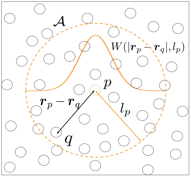
Figure A1 Graphical representation of the SPH kernel $W\left(\right|{\mathit{r}}_{\mathrm{p}}-{\mathit{r}}_{\mathrm{q}}|,l_{\mathrm{p}})$ (solid orange line), the smoothing length l_p (red arrow), the particle p, the neighbouring particles q, the support domain 𝒜 (dashed orange line), and the distance between any neighbour particle q and the particle p within the support domain r_p−r_q (black arrow). Note that particles are points in space and that their size in this schematic is arbitrary.

From the above approximations, we reformulate differential operators relevant to our study in their discrete SPH forms. We write the divergence of a vector field (V), the divergence of a tensor (T) and the gradient of a vector field (V) (Monaghan, 2005) as (see Appendix B for complete derivation)

$$\begin{array}{}\text{(A5)}& {\displaystyle }(\mathrm{\nabla }\cdot \mathit{V}{)}_{\mathrm{p}}={\displaystyle \frac{\mathrm{1}}{{\mathit{\rho }}_{\mathrm{p}}}}\sum _{q=\mathrm{1}}^N{m}_{\mathrm{q}}(\mathit{V}\left({\mathit{r}}_{\mathrm{q}}\right)-\mathit{V}\left({\mathit{r}}_{\mathrm{p}}\right))\cdot {\mathrm{\nabla }}_{\mathrm{p}}{W}_{\mathrm{pq}},\text{(A6)}& {\displaystyle }(\mathrm{\nabla }\cdot \mathit{T}{)}_{\mathrm{p}}={\mathit{\rho }}_{\mathrm{p}}\sum _{q=\mathrm{1}}^N{m}_{\mathrm{q}}({\displaystyle \frac{\mathit{T}\left({\mathit{r}}_{\mathrm{q}}\right)}{{\mathit{\rho }}_{\mathrm{q}}^{\mathrm{2}}}}+{\displaystyle \frac{\mathit{T}\left({\mathit{r}}_{\mathrm{p}}\right)}{{\mathit{\rho }}_{\mathrm{p}}^{\mathrm{2}}}})\cdot {\mathrm{\nabla }}_{\mathrm{p}}{W}_{\mathrm{pq}},\text{(A7)}& {\displaystyle }(\mathrm{\nabla }\mathit{V}{)}_{\mathrm{p}}=\sum _{q=\mathrm{1}}^N{\displaystyle \frac{m_{\mathrm{q}}}{{\mathit{\rho }}_{\mathrm{q}}}}(\mathit{V}\left({\mathit{r}}_{\mathrm{q}}\right)-\mathit{V}\left({\mathit{r}}_{\mathrm{p}}\right))\otimes {\mathrm{\nabla }}_{\mathrm{p}}{W}_{\mathrm{pq}}.\end{array}$$

In Eq. (A7), ⊗ denotes the outer product. ∇_pW_pq is the gradient of the kernel at the coordinate r_p−r_q in the reference frame of particle p and is written as

$$\begin{array}{}\text{(A8)}& {\mathrm{\nabla }}_{\mathrm{p}}{W}_{\mathrm{pq}}={\displaystyle \frac{{\mathit{r}}_{\mathrm{p}}-{\mathit{r}}_{\mathrm{q}}}{|{\mathit{r}}_{\mathrm{p}}-{\mathit{r}}_{\mathrm{q}}|}}{\displaystyle \frac{\partial W\left(\right|{\mathit{r}}_{\mathrm{p}}-{\mathit{r}}_{\mathrm{q}}|,l_{\mathrm{p}})}{\partial |{\mathit{r}}_{\mathrm{p}}-{\mathit{r}}_{\mathrm{q}}|}}.\end{array}$$

Note that W_pq is a scalar function and consequently ∇_pW_pq is a vector, the inner product in Eq. (A5) is a scalar, the inner product in Eq. (A6) is a 2D vector and the outer product in Eq. (A7) is a 2D tensor of rank 2. In addition to Eqs. (A2)–(A3), the smoothing kernel must have the following set of properties to avoid nonphysical behaviour and costly computation (Liu and Liu, 2003):

$$\begin{array}{}\text{(A9)}& {\displaystyle }\begin{array}{rl}\text{compact support}:& W\left(\right|{\mathit{r}}_{\mathrm{p}}-{\mathit{r}}_{\mathrm{q}}|,l_{\mathrm{p}})=\mathrm{0},\\ & \text{ for }|{\mathit{r}}_{\mathrm{p}}-{\mathit{r}}_{\mathrm{q}}|>l_{\mathrm{p}},\end{array}\text{(A10)}& {\displaystyle }\text{positive definite}:W\left(\right|{\mathit{r}}_{\mathrm{p}}-{\mathit{r}}_{\mathrm{q}}|,l_{\mathrm{p}})\ge \mathrm{0},\text{(A11)}& {\displaystyle }\text{monotonically decreasing}:{\displaystyle \frac{\partial W\left(\right|{\mathit{r}}_{\mathrm{p}}-{\mathit{r}}_{\mathrm{q}}|,l_{\mathrm{p}})}{\partial \left(\right|{\mathit{r}}_{\mathrm{p}}-{\mathit{r}}_{\mathrm{q}}\left|\right)}}\le \mathrm{0},\text{(A12)}& {\displaystyle }\begin{array}{rl}\text{symmetric}:& W\left(\right|{\mathit{r}}_{\mathrm{p}}-{\mathit{r}}_{\mathrm{q}}|,l_{\mathrm{p}})\\ & =W(-|{\mathit{r}}_{\mathrm{p}}-{\mathit{r}}_{\mathrm{q}}|,l_{\mathrm{p}}),\end{array}\text{(A13)}& {\displaystyle }\text{differentiable}:{\displaystyle \frac{{\partial }^{n}W\left(\right|{\mathit{r}}_{\mathrm{p}}-{\mathit{r}}_{\mathrm{q}}|,l_{\mathrm{p}})}{\partial \left(\right|{\mathit{r}}_{\mathrm{p}}-{\mathit{r}}_{\mathrm{q}}|{)}^n}}\exists ,\end{array}$$

where ∃ stands for exist. In the above, “differentiable” means that the kernel derivatives exist up to the highest order present in the equations. Finally, to ensure the consistency of the discretization of partial differential equations (PDEs; as defined in Belytschko et al., 1998) of the SPH method approximations to the nth order, all kernel moments of order 1 to n need to vanish. In practice, the consistency conditions are satisfied when the number of neighbouring particles is sufficiently large to be evenly distributed in the domain of influence (Fraga Filho, 2019). Note that, at the boundaries, the domain of influence of the particle is truncated, making it impossible to satisfy the kernel moment equations. This phenomenon is referred to as the particle inconsistency and leads to poorer approximations of physical properties. No clear solutions to this problem have been proposed in the literature yet.

Appendix B: Vector operators in SPH

Vector operators take different forms in the SPH framework because they only operate on the smoothing kernel W and they need to ensure symmetric interactions between particles. The following subsections show the demonstrations to obtain the relevant one to our study.

B1 Divergence of a vector

First, the divergence of vector needs to be changed into a form that can be symmetrized. To do so, we use the identity of the divergence of a scalar function times a vector and chose the scalar function to be the density as follow:

$$\begin{array}{}\text{(B1)}& \mathrm{\nabla }\cdot \mathit{V}={\displaystyle \frac{\mathrm{1}}{\mathit{\rho }}}(\mathrm{\nabla }\cdot (\mathit{\rho }\mathit{V})-\mathit{V}\cdot \mathrm{\nabla }\mathit{\rho }).\end{array}$$

Now applying the integral interpolant approximation (A1) to the divergence term (∇⋅(ρV)) and to the density (ρ) gives

$$\begin{array}{}\text{(B2)}& {\displaystyle }\begin{array}{rl}\mathrm{\nabla }\cdot \left(\mathit{\rho }\mathit{V}\right)& =\underset{\mathcal{V}}{\int }{\mathrm{\nabla }}^{\prime }\cdot \left({\mathit{\rho }}^{\prime }{\mathit{V}}^{\mathbf{\prime }}\right)W\mathrm{d}{\mathit{r}}^{\mathbf{\prime }}=\underset{\mathcal{V}}{\int }{\mathrm{\nabla }}^{\prime }\cdot \left({\mathit{\rho }}^{\prime }{\mathit{V}}^{\mathbf{\prime }}W\right)\mathrm{d}{\mathit{r}}^{\mathbf{\prime }}\\ & -\underset{\mathcal{V}}{\int }{\mathit{\rho }}^{\prime }{\mathit{V}}^{\mathbf{\prime }}\cdot {\mathrm{\nabla }}^{\prime }W\mathrm{d}{\mathit{r}}^{\mathbf{\prime }},\end{array}\text{(B3)}& {\displaystyle }\mathit{\rho }=\underset{\mathcal{V}}{\int }{\mathit{\rho }}^{\prime }W\mathrm{d}{\mathit{r}}^{\mathbf{\prime }}.\end{array}$$

In the above equations, the prime quantities represent the surrounding values. Note that the kernel is the only function that depends on both primed and non-primed positions as defined in Eq. (A1). Using the divergence theorem, the first term in Eq. (B2) can be cancelled:

$$\begin{array}{}\text{(B4)}& \underset{\mathcal{V}}{\int }{\mathrm{\nabla }}^{\prime }\cdot \left({\mathit{\rho }}^{\prime }{\mathit{V}}^{\mathbf{\prime }}W\right)\mathrm{d}{\mathit{r}}^{\mathbf{\prime }}=\underset{\mathcal{S}}{\int }\left({\mathit{\rho }}^{\prime }{\mathit{V}}^{\mathbf{\prime }}W\right)\cdot \mathrm{d}{\mathit{s}}^{\mathbf{\prime }}=\mathrm{0},\end{array}$$

since the integration surface 𝒮 encompassing the volume 𝒱 is arbitrary and the kernel W has the compact support property (Eq. A9). Applying the particle approximation (A4) to Eqs. (B2)–(B3), we obtain

$$\begin{array}{}\text{(B5)}& {\displaystyle }\begin{array}{rl}(\mathrm{\nabla }\cdot (\mathit{\rho }\mathit{V}){)}_{\mathrm{p}}& =-\sum _{\mathrm{q}}{m}_{\mathrm{q}}{\mathit{V}}_{\mathrm{q}}\cdot {\mathrm{\nabla }}_q{W}_{\mathrm{pq}}\\ & =\sum _{\mathrm{q}}{m}_{\mathrm{q}}{\mathit{V}}_{\mathrm{q}}\cdot {\mathrm{\nabla }}_p{W}_{\mathrm{pq}},\end{array}\text{(B6)}& {\displaystyle }{\mathit{\rho }}_{\mathrm{p}}=\sum _{\mathrm{q}}{m}_{\mathrm{q}}{W}_{\mathrm{pq}},\end{array}$$

where we used the identity ${\mathrm{\nabla }}_{\mathrm{p}}=-{\mathrm{\nabla }}_{\mathrm{q}}$ and p and q represent the current particle and neighbour. Finally, substituting the last two Eqs. (B5)–(B6) into Eq. (B1) gives the desired form of the operator:

$$\begin{array}{}\text{(B7)}& {\displaystyle }\begin{array}{rl}(\mathrm{\nabla }\cdot \mathit{V}{)}_{\mathrm{p}}& ={\displaystyle \frac{\mathrm{1}}{{\mathit{\rho }}_{\mathrm{p}}}}(\sum _{\mathrm{q}}{m}_{\mathrm{q}}{\mathit{V}}_{\mathrm{q}}\cdot {\mathrm{\nabla }}_p{W}_{\mathrm{pq}}-{\mathit{V}}_{\mathrm{p}}\\ & \cdot {\mathrm{\nabla }}_{\mathrm{p}}\sum _{\mathrm{q}}{m}_{\mathrm{q}}{W}_{\mathrm{pq}})\end{array}\text{(B8)}& {\displaystyle }={\displaystyle \frac{\mathrm{1}}{{\mathit{\rho }}_{\mathrm{p}}}}\left(\sum _{\mathrm{q}}{m}_{\mathrm{q}}\right({\mathit{V}}_{\mathrm{q}}-{\mathit{V}}_{\mathrm{p}})\cdot \mathrm{\nabla }{W}_{\mathrm{pq}}).\end{array}$$

B2 Divergence of a 2D tensor field

Note that in the following demonstration, the Einstein summation convention is used to simplify the calculation and the tensor representation. We start with the divergence of a 2D tensor divided by the density:

$$\begin{array}{}\text{(B9)}& {\displaystyle \frac{\partial }{\partial x_i}}\left({\displaystyle \frac{T_{ij}}{\mathit{\rho }}}\right)={\displaystyle \frac{\mathrm{1}}{\mathit{\rho }}}{\displaystyle \frac{\partial T_{ij}}{\partial x_i}}-{\displaystyle \frac{T_{ij}}{{\mathit{\rho }}^{\mathrm{2}}}}{\displaystyle \frac{\partial \mathit{\rho }}{\partial x_i}}.\end{array}$$

Reorganizing the terms gives

$$\begin{array}{}\text{(B10)}& {\displaystyle \frac{\partial T_{ij}}{\partial x_i}}=\mathit{\rho }\left[{\displaystyle \frac{\partial }{\partial x_i}}\right({\displaystyle \frac{T_{ij}}{\mathit{\rho }}})+{\displaystyle \frac{T_{ij}}{{\mathit{\rho }}^{\mathrm{2}}}}{\displaystyle \frac{\partial \mathit{\rho }}{\partial x_i}}].\end{array}$$

Now applying the interpolant approximation (A1) to the first term in the bracket leads to

$$\begin{array}{}\text{(B11)}& {\displaystyle \frac{\partial }{\partial x_i}}\left({\displaystyle \frac{T_{ij}}{\mathit{\rho }}}\right)=\underset{\mathcal{V}}{\int }{\displaystyle \frac{\partial }{\partial x_i^{\prime }}}\left({\displaystyle \frac{T_{ij}^{\prime }}{{\mathit{\rho }}^{\prime }}}\right)W\mathrm{d}{\mathit{r}}^{\mathbf{\prime }}\text{(B12)}& {\displaystyle }=\underset{\mathcal{V}}{\int }{\displaystyle \frac{\partial }{\partial x_i^{\prime }}}\left({\displaystyle \frac{T_{ij}^{\prime }}{{\mathit{\rho }}^{\prime }}}W\right)\mathrm{d}{\mathit{r}}^{\mathbf{\prime }}-\underset{\mathcal{V}}{\int }\left({\displaystyle \frac{T_{ij}^{\prime }}{{\mathit{\rho }}^{\prime }}}\right){\displaystyle \frac{\partial W}{\partial x_i^{\prime }}}\mathrm{d}{\mathit{r}}^{\mathbf{\prime }}.\end{array}$$

As for the divergence of a vector demonstration (Sect. B1), the first integral above vanishes by using the divergence theorem, and applying the particle approximation gives

$$\begin{array}{}\text{(B13)}& \begin{array}{rl}({\displaystyle \frac{\partial }{\partial x_i}}& \left({\displaystyle \frac{T_{ij}}{\mathit{\rho }}}\right){)}_{\mathrm{p}}=-\sum _{\mathrm{q}}\left(m_{\mathrm{q}}{\displaystyle \frac{(T_{ij}{)}_{\mathrm{q}}}{{\mathit{\rho }}_{\mathrm{q}}^{\mathrm{2}}}}\right){\displaystyle \frac{\partial W_{\mathrm{pq}}}{\partial (x_i{)}_{\mathrm{q}}}}\\ & =\sum _{\mathrm{q}}\left(m_{\mathrm{q}}{\displaystyle \frac{(T_{ij}{)}_{\mathrm{q}}}{{\mathit{\rho }}_{\mathrm{q}}^{\mathrm{2}}}}\right){\displaystyle \frac{\partial W_{\mathrm{pq}}}{\partial (x_i{)}_{\mathrm{p}}}}.\end{array}\end{array}$$

Substituting this into Eq. (B10) and using the equality Eq. (B6) we get the following expression:

$$\begin{array}{}\text{(B14)}& {\displaystyle }\begin{array}{rl}({\displaystyle \frac{\partial T_{ij}}{\partial x_i}}{)}_{\mathrm{p}}& ={\mathit{\rho }}_{\mathrm{p}}\left[\sum _{\mathrm{q}}\right(m_{\mathrm{q}}{\displaystyle \frac{(T_{ij}{)}_{\mathrm{q}}}{{\mathit{\rho }}_{\mathrm{q}}^{\mathrm{2}}}}){\displaystyle \frac{\partial W_{\mathrm{pq}}}{\partial (x_i{)}_{\mathrm{p}}}}\\ & +{\displaystyle \frac{(T_{ij}{)}_{\mathrm{p}}}{{\mathit{\rho }}_{\mathrm{p}}^{\mathrm{2}}}}{\displaystyle \frac{\partial }{\partial (x_i{)}_{\mathrm{p}}}}\left(\sum _{\mathrm{q}}{m}_{\mathrm{q}}{W}_{\mathrm{pq}}\right)]\end{array}\text{(B15)}& {\displaystyle }={\mathit{\rho }}_{\mathrm{p}}\left[\sum _{\mathrm{q}}{m}_{\mathrm{q}}\right({\displaystyle \frac{(T_{ij}{)}_{\mathrm{q}}}{{\mathit{\rho }}_{\mathrm{q}}^{\mathrm{2}}}}+{\displaystyle \frac{(T_{ij}{)}_{\mathrm{p}}}{{\mathit{\rho }}_{\mathrm{p}}^{\mathrm{2}}}}\left){\displaystyle \frac{\partial W_{\mathrm{pq}}}{\partial (x_i{)}_{\mathrm{p}}}}\right]\text{(B16)}& {\displaystyle }={\mathit{\rho }}_{\mathrm{p}}\sum _{\mathrm{q}}{m}_{\mathrm{q}}({\displaystyle \frac{{\mathit{T}}_{\mathrm{q}}}{{\mathit{\rho }}_{\mathrm{q}}^{\mathrm{2}}}}+{\displaystyle \frac{{\mathit{T}}_{\mathrm{p}}}{{\mathit{\rho }}_{\mathrm{p}}^{\mathrm{2}}}})\cdot {\mathrm{\nabla }}_{\mathrm{p}}{W}_{\mathrm{pq}},\end{array}$$

which is the form presented in Eq. (A6).

B3 Gradient of a vector field

To demonstrate Eq. (A7) we first write

$$\begin{array}{}\text{(B17)}& \mathrm{\nabla }\left(a\mathit{V}\right)=a\mathrm{\nabla }\mathit{V}+\mathit{V}\cdot \mathrm{\nabla }a.\end{array}$$

Choosing a=1 and recalling that the zeroth-order moment of the kernel also equals 1, we can substitute it in the last term of the expression (B17) and obtain

$$\begin{array}{}\text{(B18)}& {\displaystyle }\mathrm{\nabla }\left(\mathit{V}\right)=\mathrm{\nabla }\mathit{V}+\mathit{V}\cdot \mathrm{\nabla }{M}_{\mathrm{0}}\text{(B19)}& {\displaystyle }=\mathrm{\nabla }\mathit{V}+\mathit{V}\cdot \mathrm{\nabla }\underset{\mathcal{V}}{\int }W(\mathit{r}-{\mathit{r}}^{\mathbf{\prime }},l_{\mathrm{p}})\mathrm{d}{\mathit{r}}^{\mathbf{\prime }}.\end{array}$$

Finally using the particle approximation (A4) we get

$$\begin{array}{}\text{(B20)}& {\displaystyle }\begin{array}{rl}(\mathrm{\nabla }\mathit{V}{)}_{\mathrm{p}}& ={\displaystyle \frac{\partial }{\partial (x_i{)}_{\mathrm{p}}}}\sum _{\mathrm{q}}{\displaystyle \frac{m_{\mathrm{q}}}{{\mathit{\rho }}_{\mathrm{q}}}}(V_j{)}_{\mathrm{q}}{W}_{\mathrm{pq}}-(V_j{)}_{\mathrm{p}}{\displaystyle \frac{\partial }{\partial (x_i{)}_{\mathrm{p}}}}\\ & \sum _{\mathrm{q}}{\displaystyle \frac{m_{\mathrm{q}}}{{\mathit{\rho }}_{\mathrm{q}}}}{W}_{\mathrm{pq}}\end{array}\text{(B21)}& {\displaystyle }=\sum _{\mathrm{q}}{\displaystyle \frac{m_{\mathrm{q}}}{{\mathit{\rho }}_{\mathrm{q}}}}\left(\right(V_j{)}_{\mathrm{q}}-\left(V_j{)}_{\mathrm{p}}\right){\displaystyle \frac{\partial }{\partial (x_i{)}_{\mathrm{p}}}}{W}_{\mathrm{pq}}\text{(B22)}& {\displaystyle }=\sum _{\mathrm{q}}{\displaystyle \frac{m_{\mathrm{q}}}{{\mathit{\rho }}_{\mathrm{q}}}}({\mathit{V}}_{\mathrm{q}}-{\mathit{V}}_{\mathrm{p}})\otimes {\mathrm{\nabla }}_{\mathrm{p}}{W}_{\mathrm{pq}},\end{array}$$

which is Eq. (A7) and where Einstein summation convention was once again used to simplify the derivation.