Aerial observations of sea ice breakup by ship waves

We provide high-resolution in situ observations of wave-induced sea ice breakup in the natural environment. In order to obtain such data, a drone was deployed from the Canadian Coast Guard ship Amundsen as it sailed in the vicinity of large ice floes in Baffin Bay and in the St. Lawrence Estuary, Canada. The footage recorded during these experiments was used to obtain the floe size distribution (FSD) and the temporal evolution of the breakup. Floe-area-weighted FSDs exhibit a modal shape, indicating that a preferential size is generated by wave-induced breakup. Furthermore, the increase of the mode of the distribution with greater thickness indicates that ice thickness plays a defined role in determining the preferential size. Comparison with relevant theory suggests that the maximum floe size is dictated not only by the ice rigidity but also by the incident wavelength. It was also observed that the in-ice wavelength is smaller than the estimated incident wavelength, suggesting that waves responsible for the breakup obey mass loading dispersion. The fact that the breakup advances almost as fast as the wave energy suggests that fatigue might not have been an important physical component during the experiments. Moreover, the observed breakup extents show that thicker ice can attenuate waves less than thinner ice. Overall, this dataset provides key information on wave-induced sea ice breakup and highlights the potential for better understanding the physics of natural sea ice in response to waves.

1 Introduction

The marginal ice zone (MIZ) is the ice-covered region that is affected by waves, usually found on the periphery of the polar and subpolar oceans. Reductions in the Arctic sea ice thickness and summer extent in response to global warming (Kwok and Rothrock, 2009; Cavalieri and Parkinson, 2012) generally contribute to increase the extent of the MIZ (Horvat and Tziperman, 2015; Squire, 2020). The decrease in the summer minimum extent at a rate of 10 % per decade over the last 30 years (Comiso et al., 2008) has provided a larger fetch to increasingly frequent cyclones (Rinke et al., 2017), which generate a more energetic wave field in the Arctic Basin (Smith and Thomson, 2016; Stopa et al., 2016; Li et al., 2019; Thomson and Rogers, 2014; Casas-Prat and Wang, 2020). The increasingly energetic waves may then have greater potential to break up sea ice, thereby generating a larger MIZ. Consequently, changes in sea ice dynamics and in ocean–atmosphere heat exchanges could be observed at the large scale.

By fracturing large pieces of sea ice into smaller ones, waves change the floe size distribution (FSD) locally and, thus, contribute to an increase in the total lateral sea ice surface that is in contact with water. This results in a greater total sea ice perimeter and in the exposure of water areas that were previously capped under a layer of sea ice to the atmosphere. During the melt season, both the increase in the total ice perimeter and the lower albedo caused by the exposure of darker waters can increase the melt rate (Steele, 1992). On the other hand, enhanced heat loss from the ocean to the atmosphere due to the creation of leads and cracks can promote ice formation under cold conditions.

A fragmented ice cover can also have a significantly different dynamical response to external forces, as discussed by Dumont et al. (2011). Herman et al. (2021) report in great detail, using high-resolution satellite imagery, how waves broke up a very large ice floe into much smaller ones and how easily they drifted and deformed in response to wind, waves and current. Floe size is also important for constraining some parameterizations of wave propagation and attenuation, although it is still unclear whether and how it is significant in reality. For instance, it determines the flexural response of the ice cover and, consequently, the possible scattering of wave energy (Squire, 2007). Wave scattering by sea ice can be important, especially when the floe size is comparable to or larger than the wavelength (Kohout and Meylan, 2008; Bennetts et al., 2010; Squire, 2018). It also determines the importance of energy dissipation through inelastic and anelastic strain (Boutin et al., 2018).

The FSD is an undoubtedly important parameter for sea ice dynamics; hence, there have been great efforts to quantify it. However, to our knowledge, there are no observational studies that directly relate the FSD to the processes that generated it in the natural environment. Most observations come from satellite or aerial imagery of Arctic and Antarctic MIZs, where observable floes have an unknown history (Weeks et al., 1980; Rothrock and Thorndike, 1984; Holt and Martin, 2001; Toyota and Enomoto, 2002; Toyota et al., 2006, 2011; Lu et al., 2008; Herman, 2010; Alberello et al., 2019; Herman et al., 2021). After identifying the boundaries of individual ice floes, either manually or using autonomous image processing algorithms, a characteristic length scale is determined and used as a metric for the floe size. The FSD is represented either as a number density (ND) or as a probability density function (PDF). The former approach, which is the most widely used, takes the form of a continuous curve relating the number of floes per square kilometres to the floe size in a cumulative or non-cumulative way (see Fig. 1 of Stern et al., 2018). In the second approach, floe size categories are given a probability of occurrence based on the frequency of observation in order to represent the FSD as a histogram. From the above-mentioned studies, it appears that, when represented as a ND, the FSD generally follows a power law of the form $n\left(d\right)\propto d^{-\mathit{\gamma }}$, where n is the number of floes with a characteristic floe size d and γ is the exponent of the power law. This type of distribution has been tied to the fractal and possibly scale-invariant morphology of fractured sea ice (Rothrock and Thorndike, 1984) and is sometimes presented as a path for understanding the broad characteristics of underlying physical processes (Herman, 2010). A review of the available FSD observations and of the power law is available in Stern et al. (2018). In summary, these observations give a large-scale view of the MIZ morphology and can provide information on the seasonal evolution of the FSD. However, both the low temporal resolution of satellite images and the sparseness of aerial observations do not allow one, for example, to capture the contribution of individual breakup events to the overall FSD.

Large-scale spectral wave–ice models (WIMs) (Dumont et al., 2011; Williams et al., 2013a, b; Zhang et al., 2016; Bennetts et al., 2017; Boutin et al., 2018; Bateson et al., 2020; Boutin et al., 2020) use a power law FSD to estimate sea ice morphological properties, such as the mean floe size. Such statistical moments are dependent on the shape of the FSD and are further used to parameterize numerous MIZ processes, such as the lateral melt. This kind of parametrization allows for the study of the effect of floe-size-dependent processes on sea ice dynamics, which represents a necessary step in improving global climate models and climate projections. However, by simplifying and idealizing how MIZ processes affect the shape of the FSD, these models do not represent a physically based solution of the MIZ dynamics but rather the effects of including an FSD obeying prescribed rules on the evolution of a sea ice cover (Herman, 2017). For example, Dumont et al. (2011), Williams et al. (2013a), Williams et al. (2013b), Boutin et al. (2018), Bateson et al. (2020) and Boutin et al. (2020) all model the influence of breakup by updating the maximum floe size (d_max) of a power law FSD, even though there is no empirical evidence showing that this is how fragmentation affects the shape of the FSD.

Focusing on the process of breakup itself, rather than on its influence on dynamics, Fox and Squire (1991) studied the propagation of strain into an ice sheet. Modelling sea ice as a thin, semi-infinite elastic plate, they reported that “the position [of maximum strain] depends crucially on ice thickness and to a lesser extent on wave period”. On the other hand, Herman (2017), by modelling the ice cover as a strip of discrete cubic-shaped grains linked by elastic bonds, reported that “breaking of a continuous ice sheet by waves produces floes of almost equal size, dependent on thickness and strength of the ice but not on the characteristics of the incoming waves”. By coupling a two-dimensional flexural breakup model to a three-dimensional model of wave scattering by circular floes, Montiel and Squire (2017) found that either a modal or bimodal FSD was generated from wave-induced sea ice breakup, which also suggested that a preferential size is generated from breakup. More recently, Mokus and Montiel (2021) created a two-dimensional hydrodynamic model for wave-induced sea ice breakup which combines linear wave theory and viscoelastic sea ice rheology in order to compute the scattering of wave by sea ice floes. Using an empirical strain threshold to define the floe size resulting from breakup, they reported that the FSD follows a lognormal distribution under realistic wave forcings, demonstrating that a preferential size is indeed generated by the process. They also showed that the median floe size evolves with both wave period and ice thickness, which is a result that partly contrasts with the findings of Fox and Squire (1991) and Herman (2017), who reported that the FSD is independent of the sea state.

In summary, there seems to be a consensus from process-based model studies towards the fact that a preferential size is generated by wave-induced sea ice breakup and that the power law observed at a large scale cannot be explained by this process alone. However, it is still unclear what the respective contributions of sea ice rigidity and wave properties are in determining the preferential size and the shape of the FSD. The question remains as to whether these theoretical conclusions are supported by field observations.

Although there have been significant efforts to model the breakup process, only few studies have approached the problem from an observational perspective (e.g. Langhorne et al., 1998; Kohout et al., 2014, 2016). Furthermore, little attention has been paid to the analysis of the resulting FSD and its possible connection to sea ice flexural rigidity and to waves properties (Toyota et al., 2011). The first anecdotal observations of wave-induced breakup were reported in Squire et al. (1995), who stated that “the width of the strips […] created by the process is remarkably consistent and appears […] to be rather insensitive to the spectral structure of the sea but highly dependent on ice thickness”. In other words, Squire et al. (1995) observed that the distance between successive cracks generated by breakup seems to be constant and independent of the sea state but rather dependent on the material properties of sea ice. This remark qualitatively supports the conclusions of Fox and Squire (1991) and Herman (2017), but quantitative analysis of observational data is required to fully test these hypotheses. More recently, Herman et al. (2018) carried out breakup experiments in large tanks where waves were generated artificially to break apart a layer of laboratory-grown ice with the goal of testing the conclusions of Herman (2017) and Squire et al. (1995) on the independence of the breakup pattern on wave properties. Herman et al. (2018) compared the mean sizes obtained from the experiments to a theoretical fracture distance x^* derived by Mellor (1986), which is solely dependent on the flexural rigidity of the ice. For a group of experiments (group A test 2060), the value of x^* was close to the mean size which lead Herman et al. (2018) to conclude that “the floe size resulting from breaking by waves depends not on the incoming wavelength, but rather on the mechanical properties of the ice itself”. Unfortunately, a factor of $\frac{\mathrm{1}}{\mathrm{2}}$ was omitted in the mathematical expression of x^* (as is demonstrated in Sect. 5.1) so that this conclusion needs to be revisited. Hence, observations of wave-induced sea ice breakup in the natural environment are needed, as available laboratory and field studies do not paint a complete picture of the respective role of sea ice and wave properties in determining the shape and extent of the FSD arising from this process.

To date, few field studies on natural breakup have been conducted, mainly because the MIZ is an arduous area to sample directly from. It is indeed hard to be in the MIZ at the right place and at the right time, with good but not overly harsh weather conditions for breakup to happen, and with the right apparatus and available people to measure all relevant variables during a natural breakup event. Indeed, it is possible to study wave–ice interactions in the laboratory, but it is not clear if the results directly apply to the natural environment owing mostly to the complex life history of naturally grown sea ice compared with the more homogeneous growth conditions of the laboratory.

Rather than waiting for the stars to be aligned in the natural environment, we chose to create waves with a ship in order to simulate breakup events. With the help of an unmanned aerial vehicle (UAV or drone) and image processing, the breakup experiments conducted in the Gulf of St. Lawrence (GSL) and in northern Baffin Bay (NBB) allowed us to measure the outcome of small-period waves breaking naturally grown sea ice. While no apparatus measuring curvature of the ice or incident wave properties were successfully deployed, it was possible to extract information about the resulting FSD, the breakup speed and its extent. When compared to thin elastic plate theory, these results give insight on the underlying physics of wave-induced sea ice breakup.

2 Methods

The setup for the experiments conducted to obtain FSDs resulting from wave-induced breakup is as follows. First, a large, level ice floe with a side exposed to open water is identified. A UAV is then deployed and positioned above the ice edge to record high-resolution footage of the breakup event. Finally, the Canadian Coast Guard ship (CCGS) Amundsen cruises near the floe edge at a high and constant speed such that waves are generated in the vicinity of the ice. Two experiments were carried out: the first one in February 2019 in the GSL and the second in August 2019 in NBB. In both experiments, no wind-generated wave nor swell were present; hence, the observed breakup can only be attributed to ship-generated waves. The use of a ship for these experiments provides a better management of weather conditions for drone deployments while still allowing the study of breakup in the natural environment. Such a setup also allows one to have no constraint on the location of deployments and to search for the right sea ice to break. A DJI Mavic 2 Pro was used for both experiments because of its autonomy, resilience to cold temperatures, hovering stability and high-resolution camera. The camera has a 65.5^∘ field of view and a sensor that records photos at a resolution of 20 MP as well as 4K videos. The camera is factory-calibrated by DJI. While its height relative to the takeoff location is obtained by a barometric sensor, it uses both GPS and GLONASS for geopositioning, hovering in a still position and correcting its altitude. The error on its vertical and horizontal position are 0.5 and 1.5 m, respectively. The specifics of each experiment are described below.

2.1 Gulf of St. Lawrence

The first experiment was conducted in the northwestern Gulf of St. Lawrence (GSL; 49.584^∘ N, 66.152^∘ W), Canada, on 7 February 2019, which was a clear, calm and cold day ($T_{\mathrm{air}}=-\mathrm{7.2}$ ^∘C). According to the ice chart produced by the Canadian Ice Service (CIS) on the same date, there was a $\mathrm{9}/\mathrm{10}$ sea ice concentration that consisted of grey ($\mathrm{4}/\mathrm{10}$) and grey-white ice ($\mathrm{5}/\mathrm{10}$). These stages of development are associated with thicknesses between 10 and 30 cm. The thickness of the floe that we selected for the experiment was estimated visually by looking at the ice-free board from the lower deck of the ship at ∼ 3 m above the surface (as it was not possible to directly measure the ice thickness). Given the available information and the level of uncertainty, we estimate the thickness of the ice floe as 20 ± 10 cm.

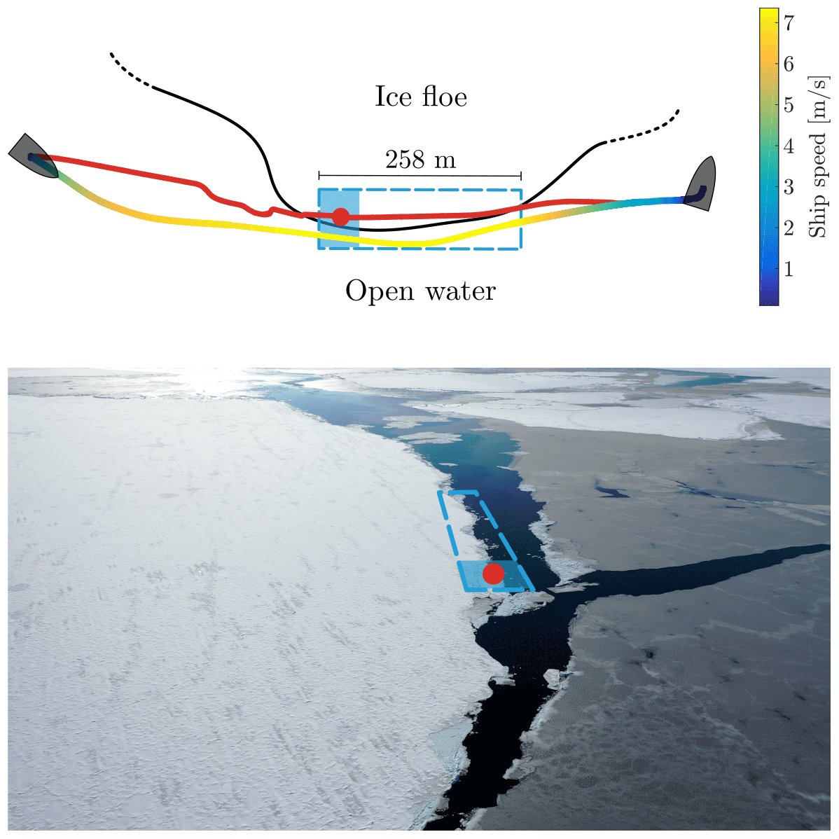
Figure 1 Schematic representation of the experiment conducted in the GSL. The grey shape represents the ship, and the red and blue-to-yellow lines are the UAV and ship GPS tracks, respectively. The red dot is the fixed position from which the drone filmed the breakup, and the filled blue rectangle is its field of view. The dashed blue rectangle is the area covered by the panoramic picture obtained by taking multiple pictures of the resulting broken ice (Fig. 7). The black line shows the approximate location of the floe edge. The bottom image is an overview of the selected floe and surrounding ice conditions.

Figure 1 shows the schematic of the GSL experiment. The CCGS Amundsen accelerated and reached an average speed of 7.25 m s⁻¹ less than 50 m from the region of interest, thereby generating a wave train with an amplitude that was sufficient to break up the ice floe. The ship speed over the portion of the trajectory that generated the observed waves remained relatively uniform, with a standard deviation of 0.08 m s⁻¹. Oblique sunlight conditions allowed us to quantify the wavelength, the period and the direction of the waves (see Sect. 3.2). Unfortunately, we could not deploy a wave sensor on the ice nor in the water; thus, we cannot quantify the wave amplitude during the experiment. A metric conversion factor of 3.1 ± 0.04 cm px⁻¹ was assessed from the UAV's altitude and field of view (FOV) by considering the manufacturers uncertainty of ±0.5 m with respect to altitude and by taking an error of ±0.5^∘ into account for the FOV.

2.2 Northern Baffin Bay

The second experiment was conducted in northern Baffin Bay (NBB; 77.883^∘ N, 77.341^∘ W) on 5 August 2019 under cloudy conditions and with an above-freezing air temperature T_air=4.9 ^∘C. According to the ice chart produced by the Canadian Ice Service (CIS) on this day, the ice concentration was $\mathrm{4}/\mathrm{10}$ and the ice thickness was identified to be between 30 and over 120 cm, as thin and thick first-year ice was indicated to be present. The floe chosen for the experiment consisted of a plate of heavily rotten first-year ice that was about 540 m wide and more than 2 km long. With the help of a Zodiac boat onboard the CCGS Amundsen, the ice thickness was measured on floes resulting from the breakup using a metrestick with a hook at one end. The thickness was assessed to be between 40 and 60 cm.

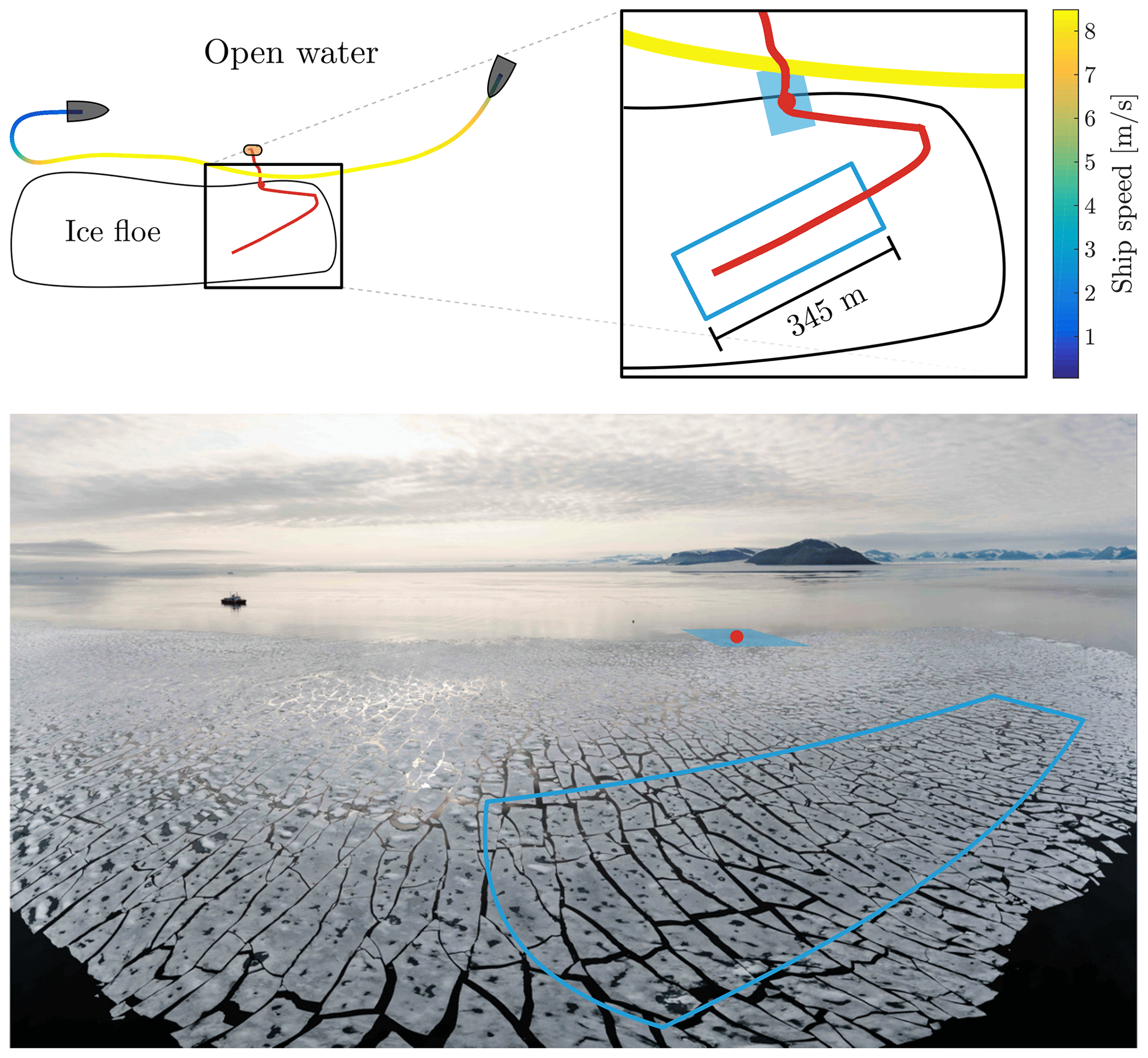
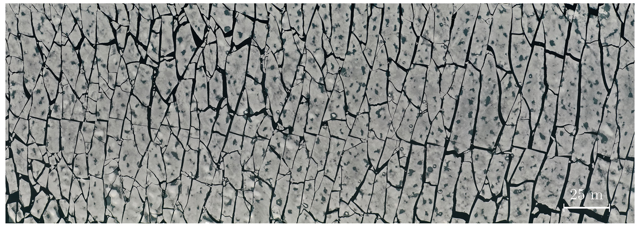
Figure 2 Schematic representation of the NBB experiment. The grey shape represents the ship, and the orange ellipse is the Zodiac. The red and blue-to-yellow lines are the UAV and ship GPS tracks, respectively. The solid and filled blue rectangles are the area of the panoramic picture selected for analysis (Fig. 8) and the FOV of the drone when the breakup was recorded, respectively. The approximate shape of the ice floe is also shown. The bottom image is an overview of the CCGS Amundsen and the selected floe after breakup.

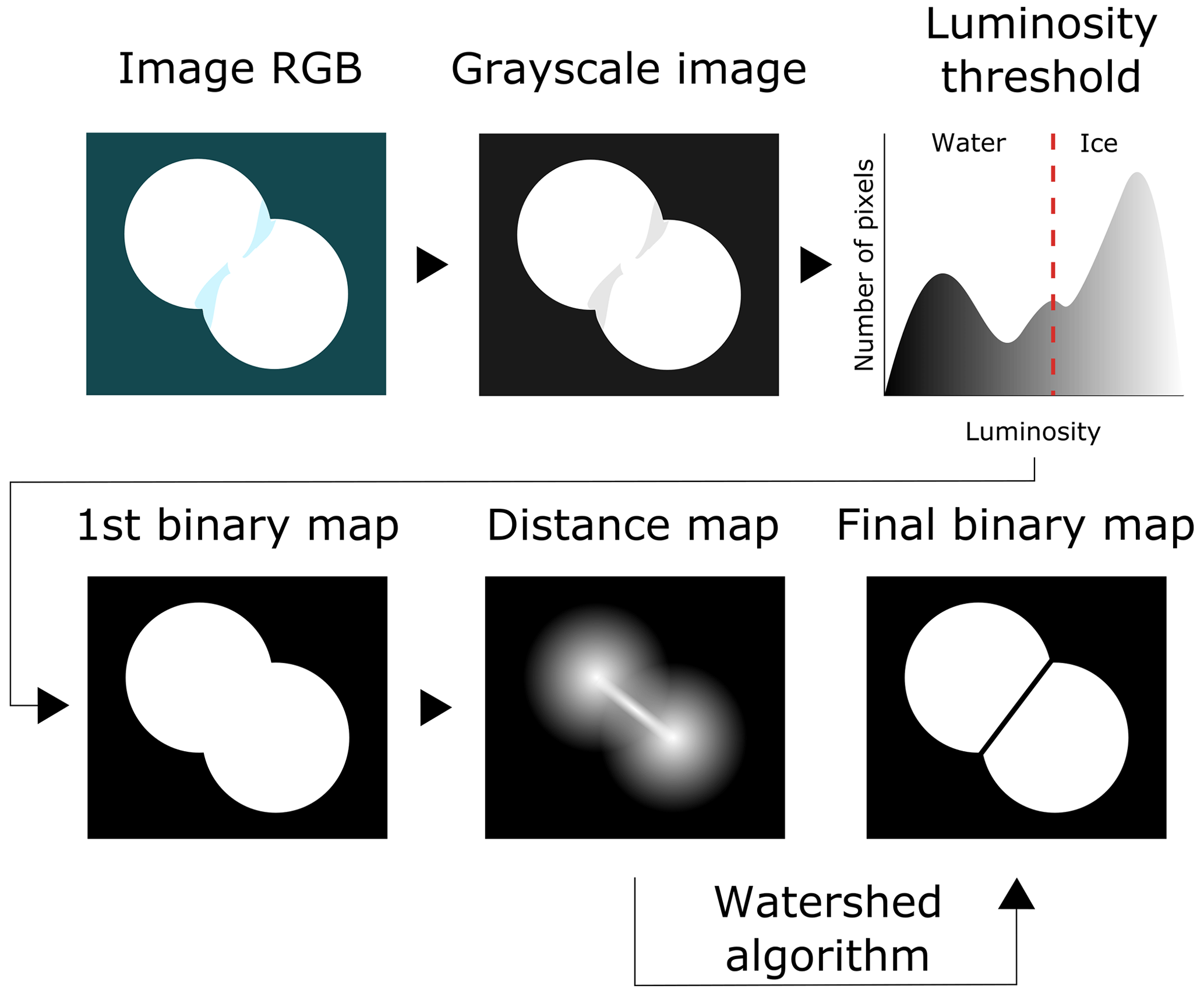
Figure 3 Steps of the image processing algorithm used for the boundary identification of floes in the GSL experiment.

Figure 2 describes the experimental setup in NBB. The average speed of the CCGS Amundsen evaluated during its passage near the floe was 8.37 m s⁻¹ with a standard deviation of 0.05 m s⁻¹. In this experiment, an attempt was made to deploy wave buoys on the ice with the Zodiac before waves hit and fractured the floe. Two surface kinematics buoys (SKIBs) (Veras Guimarães et al., 2018) were installed on the floe, 2 to 3 m from the edge and roughly 10 m apart, in order to measure the wavelength and amplitude of the waves propagating into the ice. The Zodiac then moved to a safe distance from the ice floe to launch the UAV. Unfortunately, overwash from the primary wave pushed and flipped the buoys such that their data were unusable. The propagation of flexural waves in the ice floe could not be observed visually due to the flat lighting conditions of an overcast sky. No in-ice wave properties could be measured. The UAV took pictures of the fragmented ice floe after the passage of the waves. These pictures were used to generate an orthomosaic picture of a portion of the broken floe using the open-source OpenDroneMap (ODM) software, with a resolution of 5 cm px⁻¹.

3 Image processing

3.1 Sea ice segmentation

The detection of sea ice floes in each orthomosaic consists of a series of steps, which are illustrated in Fig. 3. First the RGB image is converted to grayscale, with values from 0 to 255. From the histogram of the grayscale image, an intensity threshold separating dark water pixels from bright ice pixels is used to create a binary images where 1 indicates ice and 0 indicates water. For many reasons, this binary map does not perfectly separate ice and water nor each ice floe from their neighbours. The presence of slush or very small ice fragments in between floes can merge many floes into a larger one. Conversely, wet ice can generate holes in floes. To circumvent these imperfections, various segmentation algorithms have been developed and applied in similar contexts, namely the morphology gradient (Zhang et al., 2012), the watershed transform (Meyer, 1994; Zhang et al., 2013) or the gradient vector flow (Zhang and Skjetne, 2014, 2015). We refer the reader to Zhang and Skjetne (2018) for a good review of image processing methods that are applicable to sea ice segmentation.

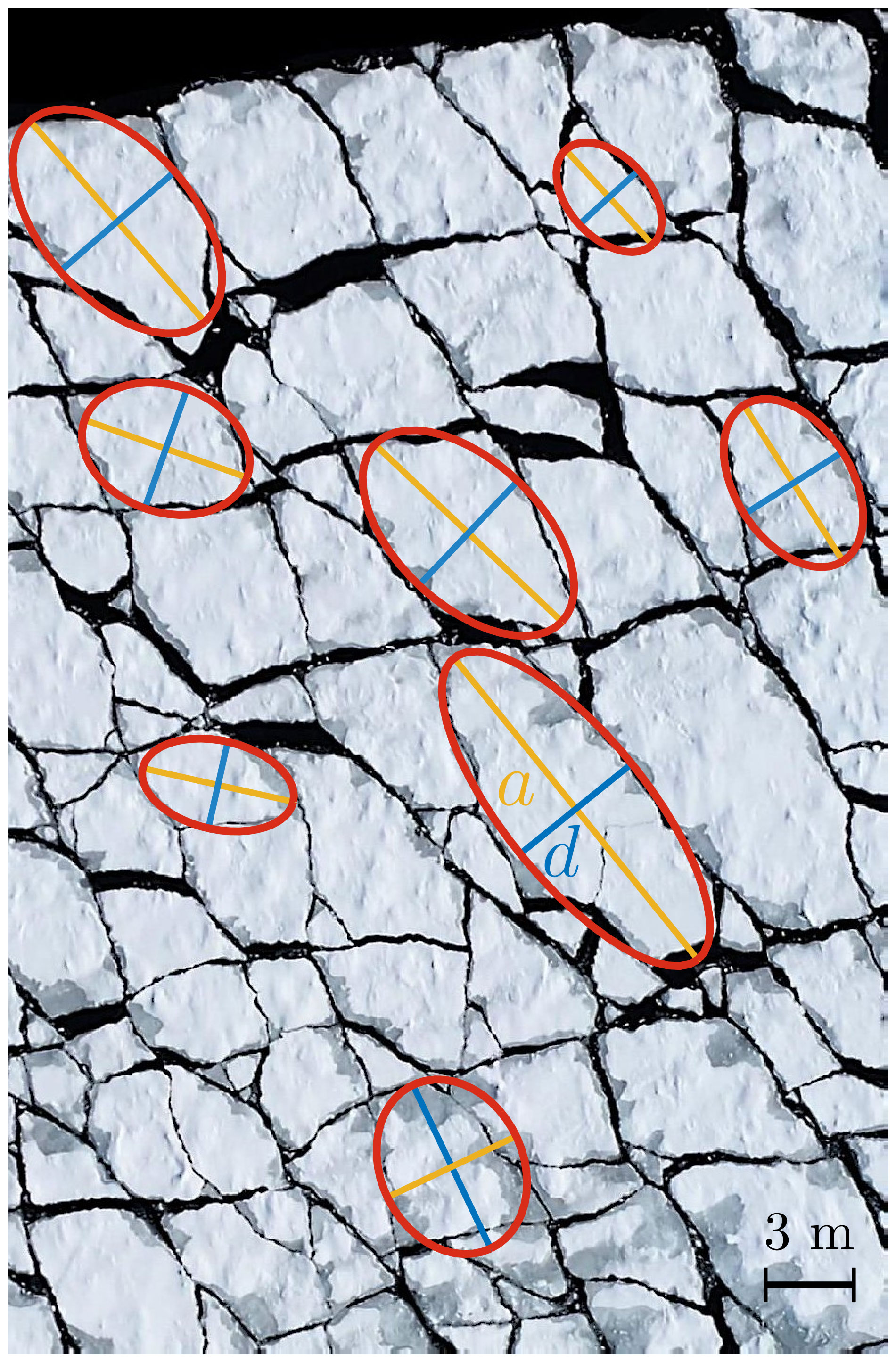
Figure 4 Sample of the ellipses fitted on the ice floes by MATLAB. Yellow and blue lines indicate the major and minor axes of length a and d, respectively.

Here, the method that gives the best results is the watershed transform (Meyer, 1994). It uses the Euclidean distance transform of the first binary map to generate a topographic map for each individual object. When two objects are in contact, the two watersheds connect through a valley. If this valley is deeper than some chosen threshold depth, the two watersheds are segmented across that valley and the original floe is separated in two. This method can sometimes generate new floes or under-segment or over-segment existing floes (Zhang and Skjetne, 2018), but it is possible to circumvent these issues with fine adjustments. To avoid over-segmentation, local minima in the distance transform are removed. To avoid under-segmentation, successive morphological erosion and dilation steps are applied to separate floes that are in contact. Finally, only objects with an isoperimetric ratio $\mathrm{\Gamma }=P^{\mathrm{2}}/\mathrm{4}\mathit{\pi }A$ smaller than or equal to 3.5 are identified as floes for further analysis.

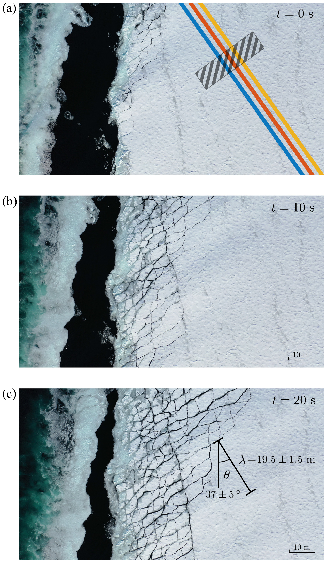
Figure 5 Snapshots of the wave-induced breakup experiment at t=0, t=10 and t=20 s. Waves are visible in the ice prior to breakup with $\mathit{\lambda }=\mathrm{19.5}\pm \mathrm{1.5}$ m. Coloured polygons in panel (a) were used to calculate the breakup speed, and the dashed rectangle is the region of interest (ROI) used for the estimation of the wave period.

Similarly to Herman et al. (2018), floes with a horizontal dimension that is close to their thickness are removed, as they cannot be generated by flexural failure. In the GSL experiment, $h=\mathrm{20}\pm \mathrm{10}$ cm. Thus, floes with a surface area A≤900 cm² are removed. For the NBB experiment, $h=\mathrm{50}\pm \mathrm{10}$ cm, and floes with A≤3600 cm² are removed. A thorough visual examination of the final binary image of the GSL experiment shows that it corresponds well to the initial image so that morphological properties of sea ice floes can be extracted from it. For the NBB experiment, the omnipresence of large melt ponds at the surface of the floes made it impossible to efficiently detect sea ice boundaries using the watershed transform method. Thus, images were manually segmented. Using the MATLAB Image Processing Toolbox, numerous morphological properties of sea ice floes are extracted. For instance, each floe is fitted to an ellipse of major axis length a and minor axis length d (Fig. 4), which is indicative of the distance between cracks induced by the highest-amplitude wave. Therefore, following Squire et al. (1995) and Herman et al. (2018), the minor axis length is chosen as the floe size, as it represents the characteristic breakup length scale.

3.2 Breakup evolution

Using drone footage in the GSL, it was possible to estimate the wavelength and the wave period due to favourable lighting conditions provided by the oblique sunlight. The in-ice wavelength λ is obtained from a visual estimation of the distance between two consecutive wave crests. The period T is obtained from a Fourier transform of the time series of the mean brightness in a region of interest (dashed rectangle in Fig. 5). The wave phase speed is then obtained by $c_{\mathrm{p}}=\mathit{\lambda }/T$.

The speed of the breakup front is evaluated using an automated and unsupervised algorithm that identifies the furthest fracture point along each of the coloured lines in the direction of wave propagation shown in Fig. 5. The algorithm computes the brightness as the mean of the image RGB values and finds the furthest pixel with a brightness value under 90, with the maximum being 255. This threshold is chosen manually after verification with a limited number of frames, and the algorithm is applied every 0.2 s. The breakup speed is then obtained as the slope of the linear regression relating the fracture distance to elapsed time.

4 Results

4.1 Waves and breakup

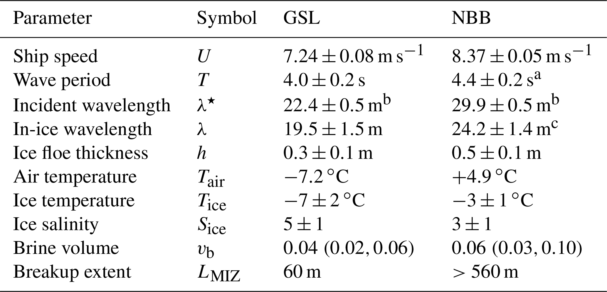
Table 1 presents a summary of the physical parameters that were measured and estimated in both experiments. In the GSL experiment, the wave period measured from brightness variations in the UAV footage is $T=\mathrm{4.0}\pm \mathrm{0.2}$ s. The in-ice wavelength is ${\mathit{\lambda }}_{\mathrm{ice}}=\mathrm{19.5}\pm \mathrm{1.5}$ m (Fig. 5). To estimate the incident wavelength and the in-ice wavelength in the NBB experiment, for which no direct measurements were made, we revert to the first-order linear Kelvin ship wake theory (Thomson, 1887). This theory states that the wavelength generated by a point source moving in a straight line at a speed U is

$$\begin{array}{}\text{(1)}& {\displaystyle }{\mathit{\lambda }}^{*}={\displaystyle \frac{\mathrm{2}\mathit{\pi }{U}^{\mathrm{2}}}{g}}{\cos }^{\mathrm{2}}\mathit{\vartheta },\end{array}$$

where ϑ is the wave angle with respect to the ship heading, and g is the gravitational acceleration. Waves generated from a moving ship can have any angle between 0 and 90^∘, but waves of maximum amplitude (a_max) propagate at an angle of $\mathit{\vartheta }{|}_{a_{\max }}={\sin }^{-\mathrm{1}}\left(\mathrm{1}/\sqrt{\mathrm{3}}\right)\simeq \mathrm{35.26}$^∘  (Soomere, 2007). As this value is within the uncertainty range of our measurement in the GSL, we use this angle for the computation of the incident wavelength for both experiments; thus, ${\mathit{\lambda }}_{\mathrm{GSL}}^{*}=\mathrm{22.4}$ m, and ${\mathit{\lambda }}_{\mathrm{NBB}}^{*}=\mathrm{29.9}$ m. Using the deepwater dispersion relation, the wave periods are then valued to T_GSL=3.8 s and T_NBB=4.4 s. These values are going to be useful later in the discussion. Note that for this theory to apply it requires that the sea state is stationary and that the ship speed is constant, which is the case in both experiments.

Figure 5 shows snapshots of wave-induced breakup in the GSL experiment. Flexure-induced cracks are parallel to the wave phase plane, which propagates at an angle of 37${}^{\circ }\pm \mathrm{5}$ with respect to the ship heading. The three coloured curves in Fig. 6 show the position of the furthest crack along the corresponding line shown in Fig. 5 as a function of time. The breakup speed is obtained as the mean slope of the three linear regressions, with a 95 % confidence interval, and is 1.86±0.04 m s⁻¹. This value is approximately 2.5 times slower than the measured wave phase speed $c_{\mathrm{p}}=\mathit{\lambda }/T\simeq \mathrm{5.0}\pm \mathrm{0.8}$ m s⁻¹.

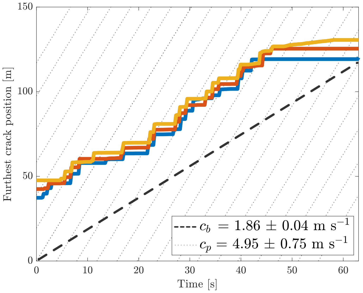
Figure 6 Temporal evolution of the furthest crack location relative to the floe edge at x=0 along the three coloured polygons shown in Fig. 5. Dotted lines indicate the position of wave crests, and the slope of the bold dashed line is obtained from the linear regression.

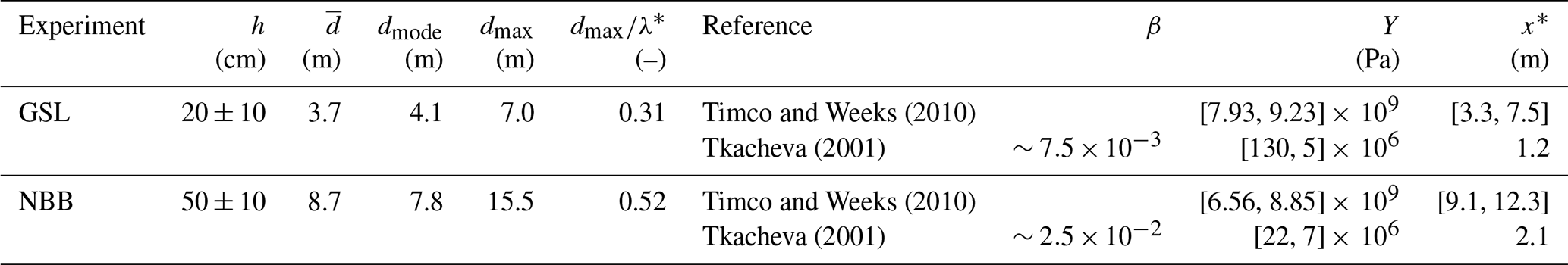
Table 1 Wave and ice parameter values measured, estimated or calculated for both experiments as well as their associated uncertainties. Values in parentheses indicate extreme values whenever they are not equidistant from the mean.

^a Estimated using the Kelvin theory (Eq. 1) and the deepwater dispersion relation ω²=gk. ^b Estimated using Eq. (1) with $\mathit{\vartheta }{|}_{a_{\max }}$ and respective ship speeds U. ^c Estimated using the mass loading dispersion relation (Eq. 16).

In the GSL, the ice fractured up to 60 m from the ice edge, leading to a partial breakup of the floe. In the NBB experiment, the 540 m wide floe was completely broken up by the ship-generated waves. Figure 7 shows the breakup that was captured by the UAV shortly after the passage of the ship (parallel to the horizontal axis of the of the image) in the GSL. Figure 8 shows only a part of the broken up floe in NBB, where the floe was too large to be mapped entirely. In both images, one can distinguish that the largest floes have a preferential size, that the crack pattern is quite homogeneous, and that floes have various sizes and shapes with sharp corners. Those are clear signs indicating that they have been broken up by the bending of surface waves.

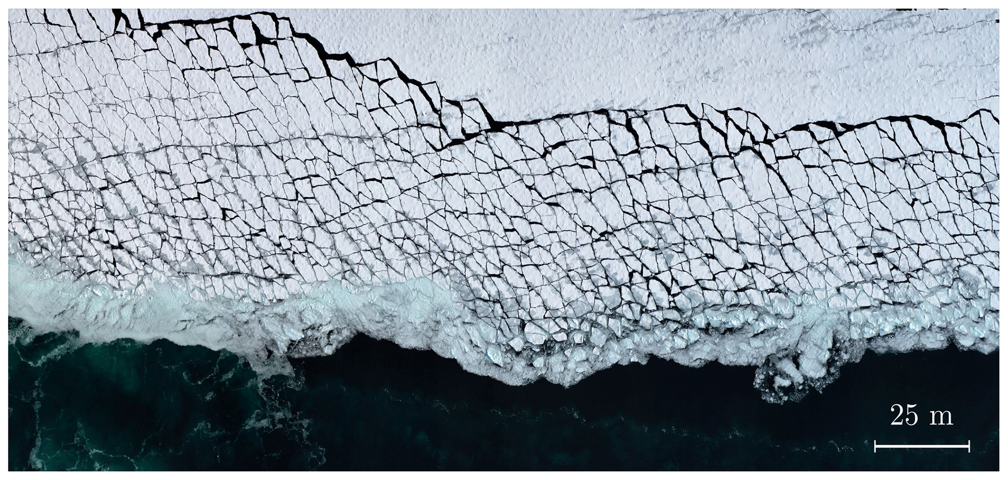
Figure 7 Breakup resulting from the GSL experiment. The ship sailed along the horizontal axis of the image.

Figure 8 Partial view of the breakup resulting from the NBB experiment, corresponding to the green rectangle in Fig. 2.

4.2 FSD as a number density

To quantify the morphology of sea ice floes, the floe size distribution is first computed using the number density, as has been done in most studies for decades (e.g. Rothrock and Thorndike, 1984; Toyota et al., 2006; Herman et al., 2021). The metric used as the floe size is the minor axis d, as it is a good approximation of the distance between cracks, which represents the linear length scale generated by the breakup (Herman et al., 2018). To build the distribution, we first determine a certain number (M) of size categories (d_i), where i=1 … M. To make sure that the result remains independent of the binning, we follow the normalization proposed by Stern et al. (2018) and set the number of bins $M=\sqrt{N}$, with N being the total number of floes. The constant bin width Δd is set equal to the size range divided by the number of bins (i.e. $\mathrm{\Delta }d=(d_{\max }-d_{\min })/M$). The probability density function computed from the number density, referred to as the NFSD, is then given by

$$\begin{array}{}\text{(2)}& P_N\left(d_i\right)={\displaystyle \frac{n_i}{N\mathrm{\Delta }d}},\sum _{i=\mathrm{1}}^M{P}_N\left(d_i\right)\mathrm{\Delta }d=\mathrm{1}.\end{array}$$

Figure 9 shows the NFSDs resulting from both experiments.

The GSL NFSD exhibits a modal shape with a mean value of 2.8 m and a standard deviation of 1.2 m. The NBB NFSD, on the other hand, has a bimodal shape with a mean value of 5.9 m and a standard deviation of 3.4 m. It is interesting to see that the NBB FSD has a shape similar to what Herman et al. (2018) obtained in a laboratory wave-induced ice fracture experiment (more precisely in their test group A 2060), which was interpreted as the sum of a power law and a Gaussian distribution. However, when looking at Figs. 7 and 8, one can see that the area is mostly covered by large floes of a similar size with a large number of very small ice fragments filling the cracks between the larger floes. The underestimation of the probabilities of finding a large floe in Fig. 8 comes from the fact that the NFSD weighs each floe equally, whereas a visual assessment puts more weight on larger floes because they cover a larger portion of the image than small floes.

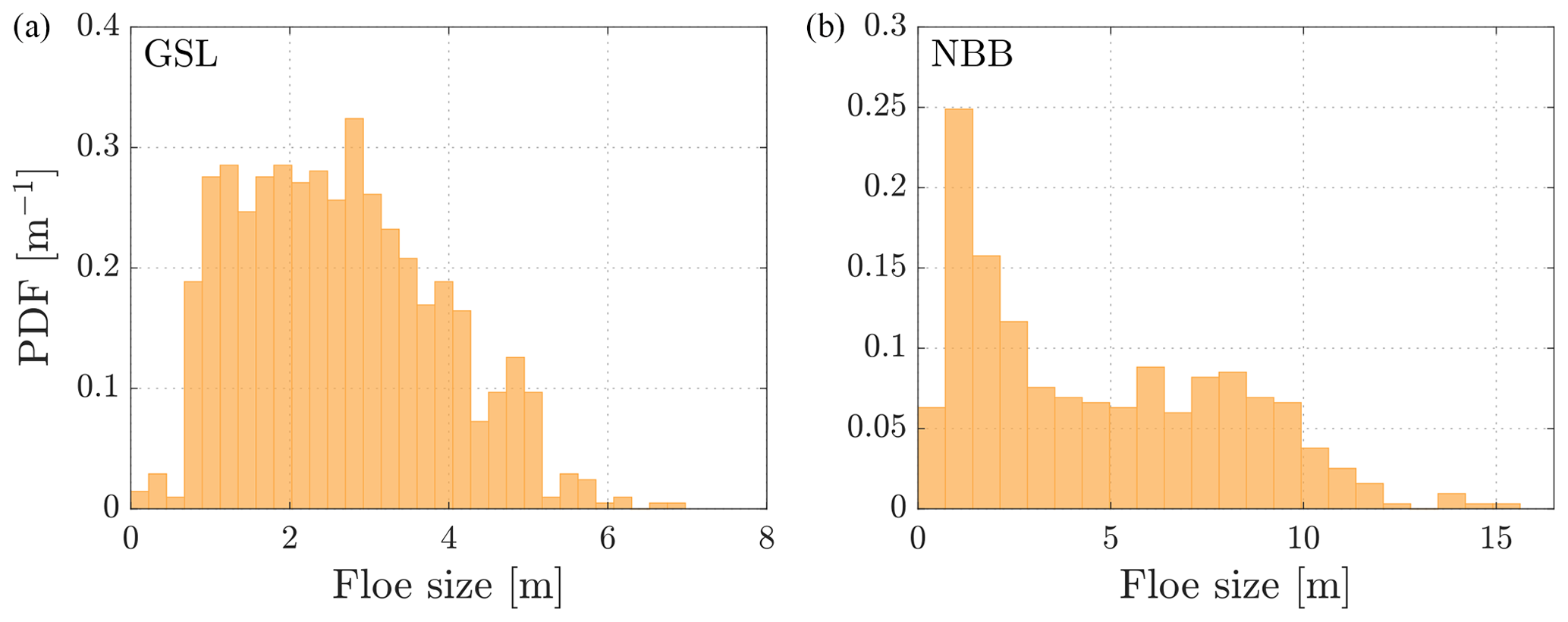
Figure 9 Number-based probability density functions of floe size (NFSDs) resulting from the breakup experiments.

4.3 Using the partial aerial concentration to compute the FSD

Let A be the total area covered by ice floes such that $A={\sum }_{k=\mathrm{1}}^N{a}_k$, where a_k is the area of floe $k=\mathrm{1},\mathrm{\dots },N$. Here, we consider the probability of a given ice pixel in the image belonging to floe k to be directly related to its partial aerial concentration $a_k/A$. Hence, the bigger the floe, the higher the probability. Following the same procedure as for the number-based PDF for the binning, the probabilities are obtained as follows:

$$\begin{array}{}\text{(3)}& {\displaystyle }{P}_A\left(d_i\right)={\displaystyle \frac{\mathrm{1}}{\mathrm{\Delta }d}}\sum _{j=\mathrm{1}}^{n_i}{\displaystyle \frac{a_j}{A}},\sum _i{P}_A\left(d_i\right)\mathrm{\Delta }d=\mathrm{1},\end{array}$$

where a_j is the area of the jth floe belonging to the ith size bin. This representation, which we call the area-based floe size distribution (AFSD), is not only compatible with a visual evaluation of an arrangement of flat plates on a surface, it is also compatible with the definition of the ice thickness distribution (ITD) that is widely used in sea ice models to characterize the state of the ice cover over a given area (Hunke and Lipscomb, 2010). More recently, the FSD has also been defined that way in a large-scale coupled wave–ice model (Boutin et al., 2020). Using this approach to build the FSD therefore makes its shape directly translatable from observations to models, like the model of Boutin et al. (2020), which currently employs the NFSD shape because it is the only shape available from observations. Unfortunately, using the minor axis as the floe size implies that information on the floe shapes is lost. Hence, computing the total area of sea ice from the NFSD is bound to be non-conservative and dependent on the assumed floe shape – a problem which is solved using the AFSD.

Figure 10 shows the AFSD for both experiments. By comparing Figs. 9a and 10a to Fig. 8, it is clear that the AFSD is more coherent with what can be seen in the orthomosaic than the NFSD is. The modal floe size for the GSL experiment is slightly shifted towards larger values with the AFSD (Fig. 10) compared with the NFSD (Fig. 9). It is worth noting here that the AFSD is much more robust to segmentation errors than the NFSD, as small artefact floes generated during the segmentation process are given a much smaller weight.

Figure 10 Area-based floe size distributions (AFSDs) resulting from the breakup experiments computed with Eq. (3). The maximal floe size is compared to λ^*, the incident wavelength of the highest-amplitude ship-generated wave estimated using Eq. (1), and to x^*, the flexural rigidity length scale given by Eq. (10) with values of Y derived from Tkacheva (2001).

5 Discussion

There are very few reports in the literature on wave-induced sea ice breakup events and even fewer that are observed at adequate time and spatial scales. The two experiments presented here, carried out under two contrasting sets of environmental conditions, shed light on multiple aspects of wave–ice interactions: (1) the floe size distribution that results from wave-induced breakup, (2) wave propagation in sea ice and (3) wave attenuation, all of which are discussed below.

5.1 Wave-induced floe size distribution

The AFSDs obtained in this study (Fig. 10) follow modal distributions, meaning that a preferential size results from wave-induced sea ice breakup, confirming what was obtained by process-based modelling studies (e.g. Fox and Squire, 1991; Herman, 2017; Montiel and Squire, 2017; Mokus and Montiel, 2021) and what was anecdotally reported by Squire et al. (1995). The shape of the AFSDs also highlights the fact that this process alone does not explain the power law distributions observed at a larger scale, where sea ice is potentially influenced by many different mechanisms and events. Additionally, the mean value $\stackrel{\mathrm{‾}}{d}$ of the AFSD increases with thickness: ${\stackrel{\mathrm{‾}}{d}}_{\mathrm{GSL}}=\mathrm{3.57}$ m with $h_{\mathrm{GSL}}\in [\mathrm{10},\mathrm{30}]$ cm, whereas ${\stackrel{\mathrm{‾}}{d}}_{\mathrm{NBB}}=\mathrm{9.00}$ m with $h_{\mathrm{NBB}}\in [\mathrm{40},\mathrm{60}]$ cm, suggesting, as in a number of previous studies (e.g. Fox and Squire, 1991; Squire et al., 1995; Herman, 2017), that the preferential floe size obtained from wave-induced sea ice breakup is influenced by sea ice thickness.

Another quantity associated with the FSD that is often used as a state variable in wave–ice interaction modelling studies (e.g. Dumont et al., 2011; Williams et al., 2013a; Bateson et al., 2020) is the maximum size d_max. Different theoretical frameworks have been proposed to relate the maximum size to a relevant physical length scale in the hope of identifying the underlying physical processes involved. Let us recall here the two main hypotheses that exist in the literature.

The first hypothesis is the one used by Dumont et al. (2011) in their wave–ice interaction model. Their parameterization considered that the maximum floe size is the distance between two consecutive locations of maximal flexural strain in a semi-infinite ice floe. In order to compute strains, they assumed that sea ice is thin and homogeneous through its thickness so that it can be considered as an Euler–Bernoulli beam that conforms to a monochromatic sinusoidal wave described as $\mathit{\eta }(x,t)=a\sin (\mathit{\omega }t-kx)$. The flexural strain (ε) applied at a given time on the ice surface is therefore

$$\begin{array}{}\text{(4)}& {\displaystyle }\mathit{\epsilon }={\displaystyle \frac{h}{\mathrm{2}}}{\displaystyle \frac{{\partial }^{\mathrm{2}}\mathit{\eta }}{\partial x^{\mathrm{2}}}}=-{\displaystyle \frac{a{k}^{\mathrm{2}}h}{\mathrm{2}}}\sin (kx-\mathit{\omega }t),\end{array}$$

where ω is the wave angular frequency, k is the wavenumber, a is its amplitude and h is the ice thickness. Taking the first-order derivative of Eq. (4) and setting it to zero gives the location of strain extrema, which are separated by a distance of $\mathit{\lambda }/\mathrm{2}$ (Dumont et al., 2011). This approach assumes that the breakup occurs after a monochromatic wave has propagated into an unbroken ice plate, at many places within the ice plate simultaneously, and far from the stress-free edge.

Another theoretical framework that has been used in the last decade in the wave–ice interaction community (e.g. Toyota et al., 2011; Williams et al., 2013a; Herman, 2017; Boutin et al., 2018; Bateson et al., 2020) is the one described by Mellor (1986) based on Hétenyi (1946), in which an analytical solution for the position x^* of the maximum bending moment in a beam subject to a downward force at its edge is derived. As an arithmetic error is present in the derivation made by Mellor (1986), which was underlined by Boutin et al. (2018), we deemed it important to recall the derivation of x^*.

First, Hétenyi (1946) considers a semi-infinite Euler–Bernoulli beam of uniform thickness h that extends along the x axis. When submitted to a load P acting downwards at its edge, a vertical deflection of the edge is generated and imposes a bending moment M along the beam defined as

$$\begin{array}{}\text{(5)}& {\displaystyle }M=-EI{\displaystyle \frac{{\partial }^{\mathrm{2}}\mathit{\eta }}{\partial x^{\mathrm{2}}}},\end{array}$$

where E and I are the elastic modulus and the second moment of area of the beam (i.e. its massless inertia), respectively (Hétenyi, 1946). Considering a stress-free condition at the edge and that M vanishes for large x, the general solution is

$$\begin{array}{}\text{(6)}& {\displaystyle }M=-{\displaystyle \frac{P}{\mathit{\mu }}}{e}^{-\mathit{\mu }x}\sin \mathit{\mu }x,\mathit{\mu }={\left({\displaystyle \frac{k_{\mathrm{f}}}{\mathrm{4}EI}}\right)}^{\frac{\mathrm{1}}{\mathrm{4}}},\end{array}$$

where k_f is the foundation modulus, which can be viewed as a Hooke's constant, and x is the axial direction of the beam (Hétenyi, 1946). Setting the first-order derivative of Eq. (6) with respect to x to zero, we obtain the following algebraic equation:

$$\begin{array}{}\text{(7)}& {\displaystyle }{e}^{-\mathit{\mu }x}(\cos \mathit{\mu }x-\sin \mathit{\mu }x)=\mathrm{0},\end{array}$$

which is satisfied when x→∞ or when $x=(\mathrm{4}n+\mathrm{1})\mathit{\pi }/\mathrm{4}\mathit{\mu }$, with $n=\mathrm{0},\mathrm{1},\mathrm{2},\mathrm{\dots }$. This implies that the location of the maximum bending moment, and therefore of maximal deformation, is

$$\begin{array}{}\text{(8)}& {\displaystyle }{x}^{*}={\displaystyle \frac{\mathit{\pi }}{\mathrm{4}}}{\left({\displaystyle \frac{\mathrm{4}EI}{k_{\mathrm{f}}}}\right)}^{\mathrm{1}/\mathrm{4}}.\end{array}$$

Even though x^* is derived for an Euler–Bernoulli beam, the second moment of area I of a Kirchhoff–Love plate is used and the Young's modulus (noted Y) is set to be equivalent to the elastic modulus E of the plate. Thus, we have

$$\begin{array}{}\text{(9)}& {\displaystyle }E=Y,I={\displaystyle \frac{h^{\mathrm{3}}}{\mathrm{12}(\mathrm{1}-{\mathit{\nu }}^{\mathrm{2}})}},\end{array}$$

which implies that

$$\begin{array}{}\text{(10)}& {\displaystyle }{x}^{*}={\displaystyle \frac{\mathit{\pi }}{\mathrm{4}}}{\left({\displaystyle \frac{Y^{*}{h}^{\mathrm{3}}}{\mathrm{3}{\mathit{\rho }}_{\mathrm{w}}g(\mathrm{1}-{\mathit{\nu }}^{\mathrm{2}})}}\right)}^{\mathrm{1}/\mathrm{4}}.\end{array}$$

Here, ν=0.3 is the Poisson ratio, ρ_w≃1025 kg m⁻³ is the seawater density and g is the gravitational acceleration. Another consideration made here is that, as the plate lies on water, the foundation modulus was set to ρ_wg.

Mellor (1986) used this framework for determining a flexure-induced fracture distance in the context of ice rafting, not for the case of wave-induced breakup. The aforementioned study reported that “when the ice is flexed, it will tend to break first at a distance x^* from the free edge”. This comment has led numerous wave–ice interaction studies, namely Toyota et al. (2011), to consider that x^* is “the minimum ice length at which breakup will occur due to flexure stress”, Williams et al. (2013a) to interpret x^* as “[corresponding] to the diameter below which flexural failure cannot occur” and Boutin et al. (2018) to assume x^* is the diameter “below which […] no flexural failure is possible”. However, as WIMs use $\mathit{\lambda }/\mathrm{2}$ as d_max, based on the fact that sea ice will break at extrema of deformation, should x^* not also be considered as a maximum floe length scale because it is based upon the same mathematical premise?

In order to compute x^* and compare this length scale with the observed maximum floe sizes, it is necessary to estimate the effective Young's modulus. Estimations of Young's modulus in wave–ice interaction studies (e.g. Williams et al., 2013a) are commonly based on empirical relationships. For Young's modulus, Timco and Weeks (2010) obtained

$$\begin{array}{}\text{(11)}& Y=Y_{\mathrm{0}}(\mathrm{1}-\mathrm{3.51}{v}_{\mathrm{b}}),\end{array}$$

where Y₀≃10 GPa, and v_b is the brine volume. As argued by Williams et al. (2013a), an effective value of $Y^{*}=Y-\mathrm{0.5}$ GPa must be used when a cyclic loading of a period less than 10 s is considered. Thus, Y^* might be used for calculating the flexural rigidity length scale x^*, as waves in our experiments had a period lower than 10 s. The brine volume depends on ice salinity but even more strongly on ice temperature. The warmer the ice, the larger the brine volume and the porosity. Here, we use the empirical relationship of Cox and Weeks (1983) to estimate v_b:

$$\begin{array}{}\text{(12)}& {\displaystyle }{v}_{\mathrm{b}}& {\displaystyle }={\displaystyle \frac{{\mathit{\rho }}_{\mathrm{ice}}S}{F}},\mathrm{with}\text{(13)}& {\displaystyle }F& {\displaystyle }=\left\{\begin{array}{l}-\mathrm{4.732}-\mathrm{22.45}{T}_{\mathrm{ice}}-\mathrm{0.6397}{T}_{\mathrm{ice}}^{\mathrm{2}}-\mathrm{0.01074}{T}_{\mathrm{ice}}^{\mathrm{3}}\\ \mathrm{for}-\mathrm{2}{}^{\circ }\mathrm{C}\ge T_{\mathrm{ice}}\ge -\mathrm{22.9}{}^{\circ }\mathrm{C}\\ \mathrm{9899}+\mathrm{1309}{T}_{\mathrm{ice}}+\mathrm{55.27}{T}_{\mathrm{ice}}^{\mathrm{2}}+\mathrm{0.716}{T}_{\mathrm{ice}}^{\mathrm{3}}\\ \mathrm{for}-\mathrm{22.9}{}^{\circ }\mathrm{C}>T_{\mathrm{ice}}>-\mathrm{30}{}^{\circ }\mathrm{C}.\end{array}\right.\end{array}$$

Unfortunately, the salinity of the ice was not measured during the experiments. To estimate it, we revert to the empirical study of Cox and Weeks (1974), who showed that thin and cold young ice has a typical salinity of around 5 ppt, whereas warm sea ice at the end of the melt season can have a typical salinity as low as 2 ppt. Thus, we set $S_{\mathrm{GSL}}=\mathrm{5}\pm \mathrm{1}$ and $S_{\mathrm{NBB}}=\mathrm{3}\pm \mathrm{1}$ to account for the two different situations as well as the uncertainty associated with these estimates. The ice temperature is set close to the freezing point of seawater for NBB and close to the air temperature for GSL (see Table 1). This gives $v_{\mathrm{b}}=\mathrm{0.04}(\mathrm{0.02},\mathrm{0.06})$ for GSL and $v_{\mathrm{b}}=\mathrm{0.06}(\mathrm{0.03},\mathrm{0.10})$ for NBB, with extrema values shown in parentheses. Using Eq. (11) with these parameter values, the maximum and minimum values for the effective Young's modulus values are $[Y_{\min }^{*},Y_{\max }^{*}]=[\mathrm{7.93},\mathrm{9.23}]$ GPa for the GSL experiment and $[Y_{\min }^{*},Y_{\max }^{*}]=[\mathrm{6.56},\mathrm{8.85}]$ GPa for the NBB experiment. Given these value intervals for Young's modulus and the thickness estimation and measurement made for the respective GSL and NBB, it is possible to compute x^* for both experiments (see Table 2).

It is worth mentioning that Mellor (1986) obtained x^* using a quasi-static framework; thus, as wave-induced sea ice breakup is inherently dynamic, we wonder if x^* is an appropriate scale for the phenomenon under study. Tkacheva (2001), on the other hand, studied the diffraction of a plane wave by a semi-infinite plate and focused on quantities relevant to the context of wave-induced breakup, namely the transmission coefficient and the position of maximum strain relative to wave and ice properties. One key quantity introduced in Tkacheva (2001) is the dimensionless reduced rigidity β, which is mathematically expressed as

$$\begin{array}{}\text{(14)}& {\displaystyle }\mathit{\beta }={\displaystyle \frac{\mathrm{16}{\mathit{\pi }}^{\mathrm{4}}EI}{{\mathit{\rho }}_{\mathrm{w}}g{\mathit{\lambda }}^{\mathrm{4}}}}.\end{array}$$

This quantity arises from the dimensional analysis of the boundary conditions considered for solving the velocity potential of a plane wave being diffracted by a plate. It translates to

$$\begin{array}{}\text{(15)}& {\displaystyle }\mathit{\beta }={\displaystyle \frac{\mathrm{4}{\mathit{\pi }}^{\mathrm{4}}Y{h}^{\mathrm{3}}}{\mathrm{3}(\mathrm{1}-{\mathit{\nu }}^{\mathrm{2}}){\mathit{\rho }}_{\mathrm{w}}g{\mathit{\lambda }}^{\mathrm{4}}}}\end{array}$$

under the Kirchhoff–Love plate approximation and when assuming that the elastic modulus is equal to Young's modulus. Computing β with the reference values of Young's modulus derived from Timco and Weeks (2010), the incident wavelengths and the ice thicknesses estimated for the two experiments give ${\mathit{\beta }}_{\mathrm{GSL}}\in [\mathrm{0.4},\mathrm{14.0}]$ and ${\mathit{\beta }}_{\mathrm{NBB}}\in [\mathrm{7.5},\mathrm{33.9}]$, which translate to transmission coefficients $|T{|}_{\mathrm{GSL}}\in [\mathrm{0.6},\mathrm{0.4}]$ and $|T{|}_{\mathrm{NBB}}\in [\mathrm{0.5},\mathrm{0.4}]$, respectively (see Fig. 2 of Tkacheva, 2001). These values are contradictory to what was observed: a near-perfect transmission of the ship waves into the ice plate. This contradiction can either come from a bad estimation of the ice thickness, the incident wavelength or Young's modulus. Despite the uncertainties, thickness and wavelength have been measured and estimated, and they do not allow for lower values of β. Young's modulus values, on the other hand, have been estimated from empirical relationships that might not be applicable to the sampled sea ice, which was grey and grey-white ice in the GSL and heavily rotten first-year ice in NBB. Moreover, the way waves propagated through sea ice, with an in-ice wavelength smaller than the incident wavelength (see Table 1), suggests that its elasticity is very low. Thus, an alternative method to quantify Y may be used in order to see if x^* adequately represents d_max.

Tkacheva (2001) also computed the position of maximum strain, expressed as a fraction of the incident wavelength, as a function of β (see Fig. 7 of Tkacheva, 2001). By assuming that d_max results from the rupture of the ice at the position of maximal strain, we can obtain a value of β by measuring the maximal size and dividing it by the incident wavelength. Table 2 displays values of $d_{\max }/\mathit{\lambda }$ that amount to 0.31 for the GSL and 0.52 for the NBB. These values lead to ${\mathit{\beta }}_{\mathrm{GSL}}\sim \mathrm{7.5}\times {\mathrm{10}}^{-\mathrm{3}}$ and ${\mathit{\beta }}_{\mathrm{NBB}}\sim \mathrm{2.5}\times {\mathrm{10}}^{-\mathrm{2}}$ which thus lead to transmission coefficients of over 95 % according to the derivation made Tkacheva (2001). We dismiss the possible value of β_NBB>10⁰ because it corresponds to situations in which more than 50 % of the incident wave would have been reflected.

With values of β, thickness and wavelength for each experiment, it is possible to estimate Young's modulus by inverting Eq. (15). In doing so, we obtain $Y_{\mathrm{GSL}}\in [\mathrm{5},\mathrm{130}]\times {\mathrm{10}}^{\mathrm{6}}$ Pa and $Y_{\mathrm{NBB}}\in [\mathrm{7},\mathrm{22}]\times {\mathrm{10}}^{\mathrm{6}}$ Pa, with the lower (upper) bound corresponding the highest (lowest) thickness value; these values are 1 to 4 orders of magnitude smaller than what is obtained from empirical relationships (see Table 2). Using these values to compute x^* as an indicator of d_max does not fit with observations. This suggests that the quasi-static theoretical framework of Mellor (1986) does not grasp the underlying physics of wave-induced sea ice breakup. In our opinion, it should also be considered a coincidence that x^* is close to the minimal size in Fig. 10, as it should, in principle, represent a maximum size.

Tkacheva (2001) provides interesting information relating the position of maximum strain (hence, d_max) to the sea ice rigidity and incident wavelength. However, as many models obtain modal-shaped FSDs by assuming that sea ice breaks up at the position where ε_c is reached, this quantity may be tied to the preferential size. Relating ε_c and the maximum strain to β might allow one to parametrize the wave-induced FSD with the physical properties of waves and ice as well as to identify where the preferential size comes from.

Timco and Weeks (2010)Tkacheva (2001)Timco and Weeks (2010)Tkacheva (2001)

Table 2 Physical quantities related to the AFSDs and comparison to x^* with different approaches to estimate the sea ice Young's modulus.

5.2 Breakup evolution and wave propagation

In the two experiments, ice broke up from the edge inward, with the furthest crack at a given time oriented parallel to the wave phase plane. The speed c_b at which the breakup progressed could only be measured in the GSL experiment using the UAV footage.

Figure 11a and b show the phase speed and the group-to-phase-speed ratio relative to the wavenumber, respectively. Along with the data of the GSL experiment, ice-free deepwater waves and two regimes of waves in ice, namely flexural waves travelling in a thin elastic plate and waves affected by the inertia of a floating material, obeying the so-called mass loading dispersion relation, are presented in Fig. 11. The general dispersion relation that describes these two regimes is given by (Liu and Mollo-Christensen, 1988)

$$\begin{array}{}\text{(16)}& {\mathit{\omega }}^{\mathrm{2}}=\left(gk+{\displaystyle \frac{Y{h}^{\mathrm{3}}{k}^{\mathrm{5}}}{\mathrm{12}(\mathrm{1}-{\mathit{\nu }}^{\mathrm{2}}){\mathit{\rho }}_{\mathrm{w}}}}\right){\left(\mathrm{1}+{\displaystyle \frac{{\mathit{\rho }}_{i}hk}{{\mathit{\rho }}_{\mathrm{w}}}}\right)}^{-\mathrm{1}}.\end{array}$$

Figure 11a shows that the measured phase speed of the wave propagating into the unbroken ice $c_{\mathrm{p}}\simeq \mathrm{4.95}\pm \mathrm{0.75}$ m s⁻¹ is lower than both the phase speed of deepwater and inertial-gravity waves but still within their range due to uncertainty. This result suggests that the waves responsible for the breakup, which are visible from the UAV footage, could propagate following the mass loading dispersion relation. This observation would be consistent with what Sutherland and Dumont (2018) observed in brash ice. It also supports the idea that the effective Young's modulus of the ice encountered in both experiments might have been low, as was suggested in Sect. 5.1. Figure 11b shows that the breakup speed $c_{\mathrm{b}}\simeq \mathrm{1.86}\pm \mathrm{0.04}$ m s⁻¹ is lower than the speed of inertial-gravity waves in ice $c_{\mathrm{g}}\simeq \mathrm{2.1}\pm \mathrm{0.2}$ m s⁻¹ but still within the uncertainty.

From the video footage of the GSL experiment, we can clearly see that waves were attenuated along their propagation into the ice. As attenuation reduces the wave amplitude, it would contribute to slowing down the breakup process and, hence, lead to c_b being smaller than c_g. On the other hand, it is also possible that the leading waves of the group might fatigue the ice and lower the critical strain (Langhorne et al., 1998), thereby increasing the breakup speed. Observing that c_b≤c_g suggests that attenuation had more of an influence than fatigue in the GSL experiment.

The results presented here allow for a rough analysis of the wave propagation into the ice, but there is clearly a need for more experiments in which wave propagation is adequately measured. Not only would this provide data to help identify the dispersion relation of waves propagating into ice but it would also aid quantification of the respective contributions of attenuation and fatigue to the breakup speed.

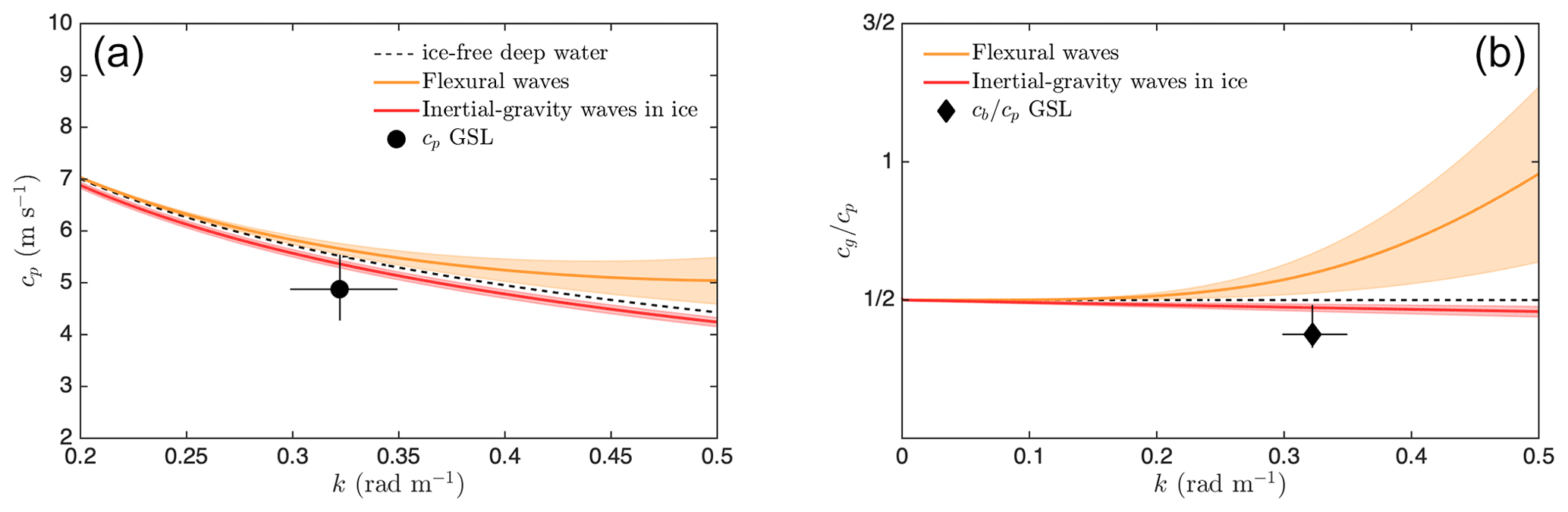
Figure 11 Phase speed (a) and the ratio between the group speed and the phase speed (b) as a function of wavenumber k for ice-free deepwater waves (dash line), pure flexural waves (orange, Eq. 16 with ρ_i=0) or pure inertial-gravity waves (red, Eq. 16 with Y=0). The mean and extreme values for ice thickness (h) and Young's modulus (Y) are those from Fig. 10 and Table 2. The black diamond indicates the ratio between the breakup speed (c_b) and the measured phase speed (c_p) in the GSL experiment, with the uncertainties described in Table 1.

5.3 Breakup extent and wave energy attenuation

In the GSL, the breakup extent reached 60 m from the original floe edge. In the NBB experiment, the entire floe that was approximately 540 m wide broke up. Assuming that the incident waves were similar in terms of period, wavelength and amplitude for both experiments (see Table 1), this suggests that the wave attenuation rate was higher (up to 1 order of magnitude) for thinner ice than for thicker ice. This might be a counterintuitive result with respect to proposed theories for wave attenuation. Far from criticizing these theories, which are meant to be applied at the large scale where waves experience averaged ice properties, this result rather suggests that wave energy dissipation or scattering depends on material properties that are not considered by models (e.g. ice porosity, temperature, heterogeneity, composition, rigidity) and are often not carefully measured in field experiments.

6 Conclusions

Results obtained from the analysis of two wave-induced sea ice breakup experiments, captured by a UAV and carried out under two contrasting sets of environmental conditions, provide direct and detailed measurements that shed light on many aspects related to wave–ice interactions. The aerial imagery of the breakup event also allowed for the characterization of wave propagation, breakup evolution and extent.

A novel way of computing the FSD – using the partial aerial concentration rather than the number density – is proposed. The AFSD allows mass conservation, as the total sea ice area can be calculated from it, which is something that cannot be achieved using the NFSD without depending on the assumed shape of the floes. Thus, we deem the AFSD to be physically more relevant than the NFSD. It is also fully coherent with numerical modelling frameworks that solve for the evolution of conserved quantities such as the ITD. The AFSD also allows one to identify the presence of a preferential floe size as a result of wave-induced breakup events. The observation of a preferential size, along with the fact that ice thickness has an effect on it, resonates with many other process-based modelling studies and anecdotal evidence reported in the literature (e.g. Fox and Squire, 1991; Squire et al., 1995; Kohout et al., 2016; Herman, 2017).

Theoretical frameworks relating the position of maximal strain to the incident wavelength (Dumont et al., 2011), to sea ice flexural rigidity (Mellor, 1986) or to both these quantities (Tkacheva, 2001) were compared against the observed AFSDs. In summary, the maximal floe size seems to be controlled by both incident wavelength and sea ice rigidity.

The estimation of the Young's modulus of the sea ice encountered during the experiments was first made using the empirical relationships of Cox and Weeks (1974), Cox and Weeks (1983), and Timco and Weeks (2010). The computed values led to an underestimation of the transmission coefficient given by Tkacheva (2001) and were, thus, considered to be incorrect estimates. Alternatively, the computation of the dimensionless rigidity (β) introduced by Tkacheva (2001) from the ratio between the observed maximal size (d_max) and the incident wavelength (λ^*) led to Young's modulus values that were not only orders of magnitude lower than the earlier estimates but that also led to transmission coefficients which were coherent with our observations. Quantification of the transmission coefficient via the measurement of the amplitudes of both the incident and in-ice waves in further experiments would allow for a better assessment of the applicability of the theoretical framework of Tkacheva (2001) in a real situation. Moreover, the development of a theoretical framework relating the location of the critical strain to wave and ice properties and the empirical identification of the critical strain are key in order to understand the physics causing a preferential size to arise from wave-induced sea breakup.

It was also identified that waves propagating into the unbroken ice might follow the mass loading dispersion relation, as the wavelength and the phase speed were smaller in unbroken ice than in deep water. Moreover, the breakup speed in the GSL experiment is less than or equal to the group speed of inertial-gravity waves, suggesting that attenuation played a bigger role than ice fatigue during the process. Finally, waves were attenuated much faster in the thinner ice floe. However, the lack of in situ data on sea ice properties and wave characteristics over the course of their propagation does not allow us to identify the processes at play nor to partition the contributions of the different processes expected to attenuate waves in ice. In summary, these results show that using a ship to generate waves allows one to experiment in a controlled yet natural environment. This is a promising way to study wave-induced sea ice breakup, which advances our understanding of numerous wave–ice interactions. Collecting key in situ data to complement the UAV information would significantly improve the scientific output. This could be done by using ice-going platforms, such as an ice canoe, to deploy wave buoys and measure ice properties (e.g. thickness, temperature, salinity, snow cover), as was done by Sutherland and Dumont (2018).