Implementing spatially and temporally varying snow densities into the GlobSnow snow water equivalent retrieval

Snow water equivalent (SWE) is a valuable characteristic of snow cover, and it can be estimated using passive spaceborne radiometer measurements. The radiometer-based GlobSnow SWE retrieval methodology, which assimilates weather station snow depth observations into the retrieval, has improved the reliability and accuracy of SWE retrieval when compared to stand-alone radiometer SWE retrievals. To further improve the GlobSnow SWE retrieval methodology, we investigate implementing spatially and temporally varying snow densities into the retrieval procedure. Thus far, the GlobSnow SWE retrieval has used a constant snow density throughout the retrieval despite differing locations, snow depth, or time of winter. This constant snow density is a known source of inaccuracy in the retrieval. Four different versions of spatially and temporally varying snow densities are tested over a 10-year period (2000–2009). These versions use two different spatial interpolation techniques: ordinary Kriging interpolation and inverse distance weighted regression (IDWR). All versions were found to improve the SWE retrieval compared to the baseline GlobSnow v3.0 product, although differences between versions are small. Overall, the best results were obtained by implementing IDWR-interpolated densities into the algorithm, which reduced RMSE (root mean square error) and MAE (mean absolute error) by about 4 mm (8 % improvement) and 5 mm (16 % improvement) when compared to the baseline GlobSnow product, respectively. Furthermore, implementing varying snow densities into the SWE retrieval improves the magnitude and seasonal evolution of the Northern Hemisphere snow mass estimate compared to the baseline product and a product post-processed with varying snow densities.

1 Introduction

Passive spaceborne microwave radiometer observations can be used to retrieve valuable information on snow cover characteristics, such as snow water equivalent (SWE) and snow depth (SD). Information about seasonal snow cover characteristics is needed in many applications; seasonal snow cover stores a large amount of freshwater, and around a sixth of the world's population is dependent on the melting snow for fresh water (Hall et al., 2008; Barnett et al., 2005). Meltwater from snow is also a significant source of hydropower (Magnusson et al., 2020), and climate model evaluation requires accurate information on snow cover characteristics (Derksen and Brown, 2012).

Passive microwave radiometer observations are often used to estimate SWE as they provide frequent repeat coverage and are mostly unaffected by different weather conditions. Spaceborne passive microwave measurements are available from 1978 onwards, meaning these measurements can be used to produce SWE retrievals that cover over 4 decades. Passive microwave SWE retrievals are usually based on a brightness temperature (T_b) gradient between two channels. T_b measurements at a frequency insensitive to dry snow (around 19 GHz) are used as a reference and compared to T_b measurements at a frequency sensitive to dry snow (around 37 GHz, the wavelength becomes comparable to the snow grain size, and there is significant volume scattering) (Chang et al., 1987; Kelly et al., 2003; Mätzler, 1994). However, the performance of SWE retrievals based on the radiometer measurements alone is limited by high uncertainties, and these retrievals do not meet user accuracy requirements with respect to retrieval skill and are poorly correlated in space and time with all other SWE products; see, for example, Derksen et al. (2005), Mudryk et al. (2015), and Mortimer et al. (2020).

An assimilation approach for SWE retrieval introduced by Pulliainen (2006) and complemented by Takala et al. (2011) that combines ground-based snow depth observations and satellite radiometer data can improve radiometer-based SWE retrievals. The assimilation-based method, also known as the GlobSnow method, has been found to produce superior results to the typical SWE retrievals based only on radiometer data (Mortimer et al., 2020). The monthly GlobSnow version 3.0 (GSv3.0) climate data record with bias correction has been used for the accurate reconstruction of the March Northern Hemisphere snow mass and its trends for the period of 1979 to 2018 (Pulliainen et al., 2020). Refining the GlobSnow SWE retrieval algorithm will improve our understanding of Northern Hemisphere snow conditions, variability, and change.

The use of a constant snow density is a known source of uncertainty in the original GlobSnow SWE retrieval (Takala et al., 2011). In the GlobSnow SWE retrieval, snow density is used to model the brightness temperatures (T_b) required to estimate effective snow grain sizes and to retrieve SD estimates. Snow density is also used to convert retrieved SD to SWE. A constant snow density value of 240 kg m⁻³ is used throughout the retrieval regardless of snow depth, location, or length of snow season. Different approaches have been tested to overcome this known source of uncertainty. Implementing the statistical snow density model presented by Sturm et al. (2010) – whereby snow densities are predicted as a function of the snow depth, day of the year, and snow class – into SWE retrieval had a negligible impact on SWE retrieval accuracy (Luojus et al., 2013). Venäläinen et al. (2021) proposed a method of using available in situ snow density data to create spatially and temporally varying snow density fields that can be used to post-process the GSv3.0 SWE retrieval product. This approach corrects the final retrieved SWE according to these spatially and temporally varying snow densities, but all instances of snow density inside (estimation of the effective snow grain size and modelling T_b) the retrieval algorithm remain unchanged. Post-processing was found to improve SWE retrieval accuracy; however, it also overcorrects SWE magnitude, especially during accumulation season (Mortimer et al., 2022). Specifically, post-processing reduces the total Northern Hemisphere snow mass when compared to the GSv3.0 snow mass, which is the opposite to the more accurate bias-corrected estimates of Pulliainen et al. (2020).

In this study, we test the implementation of dynamic snow density fields, derived from available in situ snow density data, inside the GlobSnow SWE retrieval processor with the goal of improving retrieval accuracy. We test different temporal and spatial interpolation methods and evaluate the impact of these dynamic snow densities on the effective snow grain size estimates and on the final SWE retrieval over a 10-year period (2000–2009). Our new implementation is found to improve SWE retrieval accuracy without the reduction in overall snow mass present in previous post-processing versions. The improved SWE retrieval approach will also be applied in the Copernicus Global Land Service and Horizon 2020 G3P project which strives to assess SWE conditions to improve satellite-based groundwater estimation on a global level.

2 Snow density and SWE data

SWE and snow density datasets used in this study are obtained from various sources; see Table 1 for an overview. The Eurasia data are obtained from Russia (Bulygina et al., 2011) and Finland (Haberkorn, 2019). North American snow datasets are obtained from Canada (Vionnet et al., 2021) and multiple sources in the United States. All Eurasian and some of the North American data are snow course observations. Snow course measurements consist of multiple gravimetric snow measurements made along the snow course. Measurements are averaged together, and one SWE and one snow density value are given for each location and for each day with measurements. The frequency at which snow course measurements are made varies from every 5 d (Russia during melting season) to once a month (Finland). In addition to traditional snow course measurements, the Canadian dataset contains automated measurements from snow pillows and gamma monitor (GMON) sensors. GMON sensors are based on measurements of the absorption of the natural gamma radiation through the snow cover and have a measurement footprint of 50 to 100 m² (Choquette et al., 2013). The data from Alaska and northwestern United States consist of measurements from SNOTEL stations (Serreze et al., 1999) which provide automated SWE, snow depth, precipitation, and air temperature measurements over an area of ∼9 m². SWE is measured by a snow pillow filled with an antifreeze solution. Hourly data are available from the snow pillows, but daily measurements are used as they are more robust, as hourly data are more easily affected by wind conditions and sensor issues. For snow pillow sites, we calculate snow density from SWE and snow depth. GMON measurements from locations where snow depth is also measured are used.

Table 1 An overview of SWE and snow density datasets.

These snow density and SWE datasets are divided into two parts: the first part is used for creating the spatially and temporally varying snow density fields, and the second is used for validating interpolated snow densities and retrieved SWE values. Data from Finland are used only for validation, as measurements are made only once a month, while automated data are only used for implementation. Figure 1 shows the locations of implementation (red) and validation (blue) datasets. Only manual snow courses are used for validation because they cover a larger area (500 m–4 km) and are thus more representative of the grid cell. The automated data fill in critical areas (western US) and are necessary for deriving accurate interpolated density fields. The in situ dataset used here is a significant update of that used in the previous post-processing version of Venäläinen et al. (2021) which allows for improved characterization of snow density. The northeast US data were not included in the previous work, and the Canadian dataset has been updated and expanded.

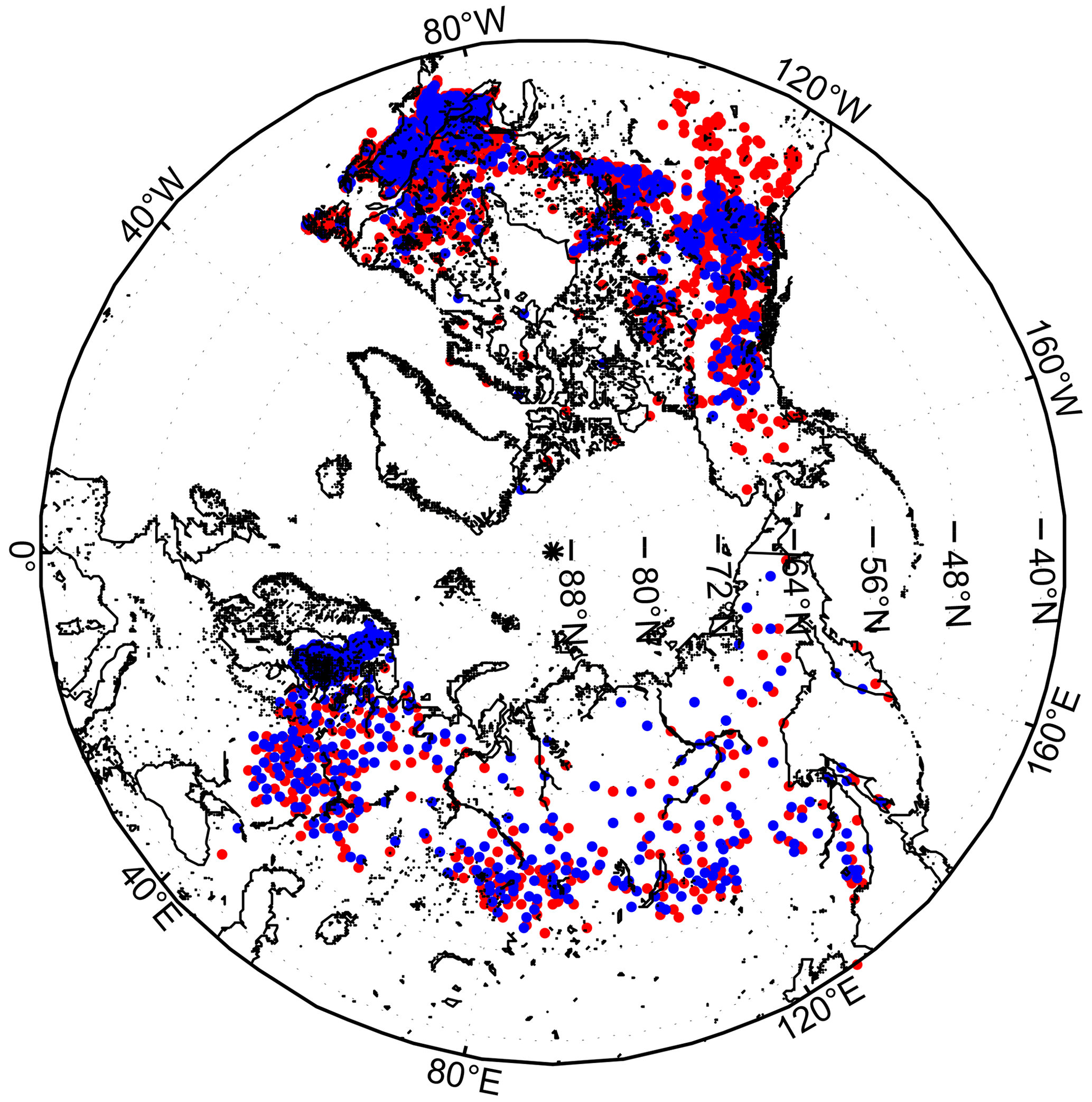
Figure 1 Snow density and SWE measurement locations. Implementation (red) and validation (blue) data are separated.

2.1 Original SWE retrieval algorithm

The GSv3.0 data record is based on the methodology introduced by Pulliainen (2006) and Takala et al. (2011), and the latest version is presented in detail in Luojus et al. (2021). The two main data inputs to the algorithm are vertical passive microwave brightness temperature (T_b) and daily synoptic snow depth (SD) measurements. The satellite T_b data are from the Special Sensor Microwave/Imager (SSM/I) and Special Sensor Microwave Imager/Sounder (SSMIS) instruments on board the Defense Meteorological Satellite Program (DMSP) F-series satellites. Measurements at 37 and 19.40 GHz (SSM/I) or 19.35 GHz (SSMIS) are used for SWE retrieval. Both synoptic SD and T_b measurements are filtered before being ingested by the algorithm. Filtering is needed to guarantee convergence on a solution during the assimilation process, and the filtering process is described in detail in Luojus et al. (2021). The main SD filtering steps include removing grid cells with a height standard deviation according to ETOPO5 (Earth topography 5 arcmin grid) greater than 200 m, removing the deepest 1.5 % of SD measurements, removing measurements from stations where the mean SD exceeds 150 m in March during at least 50 % of the years that have more than 20 annual measurements, and removing SD values above 200 cm. Water, mountain, and dry snow masking are applied to T_b measurements. SWE retrieval is performed only for dry snow, and for wet snow, the SWE estimates are based on the background SD field. Dry snow is detected using the dry snow detection algorithm by Hall et al. (2002). The GSv3.0 product is produced on a 25 km equal-area scalable grid (EASE-Grid version 1) for latitudes between 35 and 80^∘ N. The GlobSnow methodology does not produce SWE estimates for complex terrain, glaciers, or Greenland.

The four main steps of the SWE retrieval are described below; for more details see Luojus et al. (2021).

• Step 1. Ordinary Kriging interpolation is used to interpolate an “observed SD” field and interpolation variance using filtered synoptic SD observations for the day under investigation.

• Step 2. The effective snow grain size values, d₀, are retrieved for grid cells with SD observations (measurements, not interpolated values) by numerical inversion of the multi-layer HUT (Helsinki University of Technology) snow emission model. The HUT snow model expresses T_b as a function of SWE, snow density and snow grain size (Pulliainen et al., 1999). As previously mentioned, a constant value of 240 kg m⁻³ is used for snow density, as this is a reasonable global value given by the analysis of Sturm et al. (2010). The model is fit to radiometer T_b observations at the locations of SD observations by optimizing the values of d₀. The final d₀ estimate, as well as its standard deviation, at each SD measurement location is obtained by calculating the average value of the six nearest SD measurements.

• Step 3. Background d₀ field (and its variances) is interpolated from the effective snow grain size estimates produced for pixels with SD observations in step 2.

• Step 4. The bulk SWE is retrieved by ingesting observed T_b, retrieved effective snow grain sizes, grain size variances, and constant snow density (steps 2 and 3) into a numerical inversion of the HUT snow emission model. The HUT model estimates are matched to observations numerically by incrementing the SD value. The background SD field (produced in step 1) is used to constrain the retrieval. The assimilation procedure adaptively weighs the T_b measurements and the background SD field to produce a final SD estimate, converted to SWE using the constant snow density, and a measure of the statistical uncertainty (variance estimate) for each pixel:

  $$\begin{array}{}\text{(1)}& \begin{array}{rl}{\min }_{\mathrm{SD}}& \left\{{\left({\displaystyle \frac{\left(T_{\mathrm{B},\mathrm{mod}}^{\mathrm{19}v}\left(\mathrm{SD}\right)-T_{\mathrm{B},\mathrm{mod}}^{\mathrm{37}v}\left(\mathrm{SD}\right)\right)-\left(T_{\mathrm{B},\mathrm{obs}}^{\mathrm{19}v}-T_{\mathrm{B},\mathrm{obs}}^{\mathrm{37}v}\right)}{{\mathit{\sigma }}^{\mathrm{2}}}}\right)}^{\mathrm{2}}\right.\\ & \left.+{\left({\displaystyle \frac{\mathrm{SD}-{\widehat{\mathrm{SD}}}_{\mathrm{ref}}}{{\mathit{\lambda }}_{\mathrm{SD},\mathrm{ref}}}}\right)}^{\mathrm{2}}\right\},\end{array}\end{array}$$

  where ${\widehat{\mathrm{SD}}}_{\mathrm{ref}}$ is the snow depth estimate from the Kriging interpolation for the day under consideration. λ_SD,ref is the estimate of standard deviation from the Kriging interpolation, and SD is the snow depth for which Eq. (1) is minimized. The variance of T_B, ${\mathit{\sigma }}_t^{\mathrm{2}}$, is estimated by approximating $\mathrm{\Delta }{T}_{\mathrm{B}}(\mathrm{\Delta }{T}_{\mathrm{B}}=T_{\mathrm{B}}^{\mathrm{19}}-T_{\mathrm{B}}^{\mathrm{37}}$) as a function of snow depth and grain size in a Taylor series:

  $$\begin{array}{}\text{(2)}& {\displaystyle }\begin{array}{rl}\mathrm{\Delta }{T}_{\mathrm{B}}\left(\mathrm{SD},d_{\mathrm{0}}\right)& \approx \mathrm{\Delta }{T}_{\mathrm{B}}\left(\mathrm{SD},〈{\widehat{d}}_{\mathrm{0},\mathrm{ref}}〉\right)\\ & +{\displaystyle \frac{\partial \mathrm{\Delta }{T}_{\mathrm{B}}\left(\mathrm{SD},〈{\widehat{d}}_{\mathrm{0},\mathrm{ref}}〉\right)}{\partial d_{\mathrm{0}}}}\left(d_{\mathrm{0}}-〈{\widehat{d}}_{\mathrm{0},\mathrm{ref}}〉\right),\end{array}\text{(3)}& {\displaystyle }\begin{array}{rl}{\mathit{\sigma }}^{\mathrm{2}}& =\mathrm{var}\left(\mathrm{\Delta }{T}_{\mathrm{B}}\left(\mathrm{SD},〈{\widehat{d}}_{\mathrm{0},\mathrm{ref}}〉\right)\right)\\ & ={\left({\displaystyle \frac{\partial \mathrm{\Delta }{T}_{\mathrm{B}}\left(\mathrm{SD},〈{\widehat{d}}_{\mathrm{0},\mathrm{ref}}〉\right)}{\partial d_{\mathrm{0}}}}\right)}^{\mathrm{2}}{\mathit{\lambda }}_{d_{\mathrm{0}},\mathrm{ref}}^{\mathrm{2}}.\end{array}\end{array}$$

After these four main steps are performed, snow-free areas are detected and cleared of SWE to form final SWE estimate maps. The snow-free areas are detected using a combination of radiometer information and optical remote sensing snow extent information. A time-series thresholding approach by Takala et al. (2009) is used to detect the end of snowmelt, and any remaining SWE estimates are cleared from those pixels. After this, SWE estimates are also cleared from regions where optical data indicate snow-free conditions. The JASMES 5 km Snow Cover Extent data product for 1978–2018 (Hori et al., 2017) is used to construct a cumulative snow mask in a 25 km EASE-Grid projection. Cumulative masking retains the latest cloud-free observation for each EASE-Grid pixel and uses the daily product to update snow-free/snow-covered conditions, based on a 25 % snow cover fraction threshold.

2.2 Updated SWE retrieval algorithm

To improve the performance of the SWE retrieval algorithm, dynamic snow densities were inserted into the retrieval, which required some structural changes to the algorithm set-up described in Sect. 3.1. Firstly, in step 2, where the d₀ values are determined, the HUT snow emission model is given a spatially and temporally varying snow density value instead of the constant snow density. Similarly, in step 4 modelling is done with varying snow density values. Additionally, in step 4 SWE is calculated from the retrieved SD field using varying snow density information.

In step 4, SWE values are fluctuated between 0 and 350 mm to find the optimal SWE value. SWE values outside of this range can occur in instances where the background SD field (which ingests filtered data that are limited ≤200 cm) determines the estimated SWE value. When we replaced the constant snow density with a dynamic one as an input to the HUT model, anomalously high SWE values that were considerably larger than those of the surrounding pixels were retrieved for some pixels, mostly in northeast Asia. To overcome this issue, SWE is considered not to be retrieved correctly if the retrieved SWE is 80 mm larger than that estimated directly from the interpolated background SD field. In these instances, SWE is re-estimated with the range of possible SWE values set to 0 to 150 mm (comprising ∼5 % of all pixels). Figure 2 shows the general processing chain of the updated SWE retrieval algorithm. The addition of the new variable snow density information is indicated with red arrows. The four main steps described in detail are also indicated in Fig. 2.

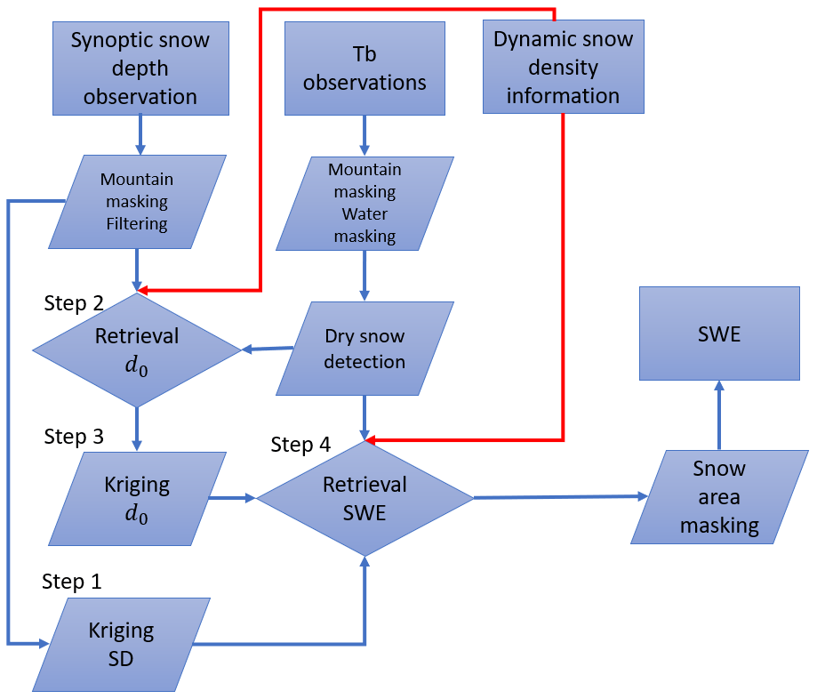
Figure 2 Processing chain of the updated SWE retrieval algorithm. The addition of dynamic snow density information is indicated with red arrows. The four main steps described in Sect. 3.1 are labelled in the figure.

3 Dynamic snow densities

Before producing the dynamic snow density fields, the available density data (described in Sect. 2) are pre-processed. First, all negative values and values larger than 1000 kg m⁻³ are removed. Then duplicate measurements are filtered by averaging density measurements within the same 25 km EASE-Grid pixel on the same date. In cases where there are exactly two measurements with large differences (more than 200 kg m⁻³), the measurement closest to the grid cell centre is used (or mean of closest measurements if multiple measurements are at the same distance) as reference. Duplicate measurements are not common, but there is some overlap between measurements from Canada and the northeast United States. Lastly, all locations in grid cells masked in the GlobSnow SWE product, primarily mountain areas, are removed.

The manual snow transects are typically only made every few weeks (Sect. 2) so temporal interpolation is necessary to fill in missing days. We tested two different implementations of temporal interpolation using the filtered snow density data: (i) a decadal version where 10-year averages are calculated for days with any snow density measurements using all data between 2000–2009 and (ii) an annual version where daily measurements or daily grid cell averages are used. We also tested two different spatial interpolation methods, ordinary Kriging interpolation and inverse distance weighted regression (IDWR), on the temporally interpolated annual and decadal datasets. Ordinary Kriging interpolation is used to interpolate background SD fields in the GlobSnow SWE retrieval, and given its successful implementation, we also tested it to interpolate snow density values. Ordinary Kriging interpolation produces variances for estimates, which are needed in the SWE assimilation procedure, but as these variance estimates are not needed for the dynamic snow density estimates, other interpolation methods can also be tested. The IDWR method was chosen because it can produce better results than the ordinary Kriging interpolation when only a limited number of measurements are available (Emmendorfer and Dimuro, 2021), which is often the case for in situ snow density. IDWR is also considerably more computationally efficient than Kriging interpolation (Longley et al., 2005). These spatial interpolation methods are described in more detail in Sect. 4.1 and 4.2. Snow density fields are produced in EASE-Grid 1.0 25 km to match the GSv3.0 product. Snow densities are estimated for the Northern Hemisphere domain even though not all locations are snow covered during the full snow season.

3.1 Kriging interpolation

Ordinary Kriging interpolation is a geostatistical interpolation method that estimates the value at an unsampled location based on the spatial autocorrelation with observed values at surrounding locations (Goovaerts, 1997). The estimated value can be calculated from a linear combination of the observed values, given by

$$\begin{array}{}\text{(4)}& {\widehat{Z}}^{\mathrm{OK}}\left(s_{\mathrm{0}}\right)=\sum _{i=\mathrm{1}}^{n}Z\left(s_i\right)w_i,\end{array}$$

where ${\widehat{Z}}^{\mathrm{OK}}\left(s_{\mathrm{0}}\right)$ is the ordinary Kriging estimated value of the variable Z (snow density) at the unsampled location s₀, and w_i is the weight set for observed measurement. The weights can be solved from the system of equations (O'Sullivan and Unwin, 2010):

$$\begin{array}{}\text{(5)}& \begin{array}{rl}& \sum _{i=\mathrm{1}}^n\mathit{\gamma }\left(d_{ij}\right)w_i+\mathit{\lambda }=\mathit{\gamma }\left(d_{jp}\right)\mathrm{for}j=\mathrm{1},\mathrm{\dots },n\\ & \sum _{i=\mathrm{1}}^n{w}_i=\mathrm{1},\end{array}\end{array}$$

where n is the number of data points, γ(d) is the semivariance between the relevant points, and λ is a Lagrangian multiplier. The constraint on weights ensures that Kriging estimates do not have systematic bias.

The variance is obtained by creating a semivariogram and then fitting the variogram model to the empirical variogram. The empirical semivariogram can be estimated from the observations as follows (O'Sullivan and Unwin, 2010):

$$\begin{array}{}\text{(6)}& \widehat{\mathit{\gamma }}\left(d_{jp}\right)={\displaystyle \frac{\mathrm{1}}{\mathrm{2}{N}_d}}\sum _{i=\mathrm{1}}^{N_{\mathrm{d}}}{\left(Z\left(s_i\right)-Z\left(s_i+d\right)\right)}^{\mathrm{2}},\end{array}$$

where Z(s_i) and Z(s_i+d) are sampled data pairs at a distance d. In this study, the fitting of the variogram is done for each day individually, separately for Eurasia and North America and using an exponential function:

$$\begin{array}{}\text{(7)}& \mathit{\gamma }\left(d\right)=c_{\mathrm{1}}\cdot \exp \left(d\cdot c_{\mathrm{2}}\right)+c_{\mathrm{0}}.\end{array}$$

3.2 IDWR interpolation

IDWR is a deterministic, non-statistical interpolation model modified from inverse distance weighting (IDW) interpolation. An IDW-interpolated value at an unsampled location is calculated as a weighted average of know values, similar to Kriging interpolation:

$$\begin{array}{}\text{(8)}& {\widehat{Z}}^{\mathrm{IDW}}\left(s_{\mathrm{0}}\right)=\sum _{i=\mathrm{1}}^{n}Z\left(s_i\right)w_i.\end{array}$$

Calculating the weights for IDW interpolation is considerably simpler than calculating weights for Kriging interpolation. IDW weights are calculated as shown below (Shepard, 1968):

$$\begin{array}{}\text{(9)}& w_i={\displaystyle \frac{d_{\mathrm{0}i}^{-\mathit{\alpha }}}{\sum _{i=\mathrm{1}}^n{d}_{\mathrm{0}i}^{-\mathit{\alpha }}}},\end{array}$$

where d is the distance between unsampled and sampled locations, and n is the number of data points available. The control parameter α is set to 2 in this study. IDW is a popular and straightforward interpolation method that is easy to implement and fast to compute (Longley et al., 2005). However, this method has some well-known limitations, including the fact that the weighting parameters are not empirically determined. Additionally, the range of the estimated values is limited by the minimum and maximum of the known values (Lam, 1983).

The IDWR modification, proposed by Emmendorfer and Dimuro (2021), introduces a new term to the IDW expression. IDWR retains the efficiency and straightforwardness of the IDW method but reduces the RMSE when compared to IDW. When the number of data points is limited, the IDWR method can produce interpolation results that are comparable to or even better than results obtained using Kriging interpolation. When more data are available, Kriging interpolation tends to produce superior results. The IDWR method estimates the value at an unsampled location as shown in Eq. (10):

$$\begin{array}{}\text{(10)}& {\widehat{Z}}^{\mathrm{IDWR}}\left(s_{\mathrm{0}}\right)={\widehat{Z}}^{\mathrm{IDW}}\left(s_{\mathrm{0}}\right)+n{\displaystyle \frac{\sum _{i=\mathrm{1}}^{n}Z\left(s_i\right)-n{\widehat{Z}}^{\mathrm{IDW}}\left(s_{\mathrm{0}}\right)}{n^{\mathrm{2}}-\sum _{i=\mathrm{1}}^n{d}_{i\mathrm{0}}^{-\mathrm{2}}\sum _{i=\mathrm{1}}^n{d}_{i\mathrm{0}}^{\mathrm{2}}}}.\end{array}$$

For a more detailed explanation of the method, see Emmendorfer and Dimuro (2021).

4 Results

In this study, we tested four different versions of dynamic snow densities inside the SWE retrieval algorithm. The first two versions use Kriging interpolation – one with decadal data and the other with annual data. These two versions allow us to test the impact of the temporal aggregation and interpolation approaches (Sect. 4). The third version uses decadal data and IDWR interpolation, and the fourth version uses annual data and IDWR interpolation. A comparison of these versions with the first two versions that use Kriging interpolation allows us to evaluate the impact of spatial interpolation methods. We first compare snow density accuracies of these four density versions (Sect. 5.1) and then evaluate their impact on snow grain size estimation (Sect. 5.2.1) and SWE retrieval (Sect. 5.2.2 and 5.2.3).

4.1 Snow densities

The derived snow density fields were validated against the validation dataset (Fig. 1, blue). The interpolated snow density values were matched with co-located snow transect snow density measurements, and bias, root mean square error (RMSE), mean absolute error (MAE), and correlation coefficient were calculated. Table 2 shows validation parameters for the four different snow density sets for 2000–2009. Table 2 also shows validation parameters for the leave one out version of decadal IDWR snow densities. This dataset is similar to decadal IDWR, but densities for each year were calculated using 9-year averages leaving out data from the year under investigation. Differences between different versions are small. For Eurasia, both annual datasets have better results than the corresponding decadal versions, and the IDWR approach outperforms ordinary Kriging interpolation. For North America, the results are the opposite, with the decadal versions producing the best results. The performance of the annual densities is worse in western North America (west of 90^∘ W) than in eastern North America (see Appendix A). In eastern North America all four density versions have similar performance. The majority of the density information in western North America comes from automated point data (snow pillows) which are less representative of the surrounding land cover and of a 25 km grid cell than snow courses are. Increasing the pool of data temporally, as is done for the decadal product, may somewhat compensate for this lack of spatial representativeness and could explain the superior performance of the decadal version in western North America.

Table 2 Summary of validation parameters for three snow density sets for 2000–2009.

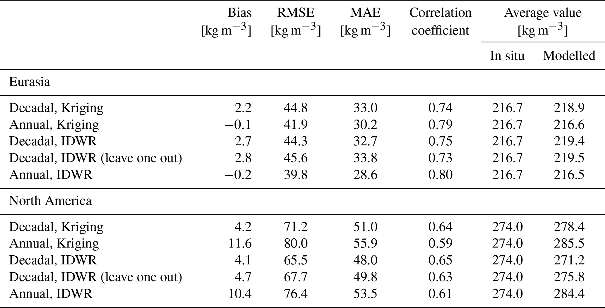
Figure 3 shows average daily snow densities for 2000–2009 for the four different snow density versions along with the constant density used in the GSv3.0 product (240 kg m⁻³). The constant density is larger than any of the varying snow densities until mid-March. After mid-March, the constant snow density is smaller than the different dynamic snow densities. Both decadal densities follow the expected progression of increased densities over the course of the snow season. In contrast, both annual density fields (Kriging and IDWR interpolated) reach a maximum in early April, after which point the snow density starts to decrease, and are lower than expected from the literature (e.g. Brown et al., 2019; Sturm et al., 2010; Sturm and Holmgren, 1998; Zhong et al., 2014). Snow courses are not conducted in extremely wet conditions or in patchy snow, so the evolution of snow density during the ablation period may not be captured in the annual datasets. However, local snow densities derived from SNOTEL snow depth and SWE have been shown to exhibit large variability during both the accumulation and ablation seasons, and oftentimes the density decreases towards the end of the ablation period (Bormann et al., 2013).

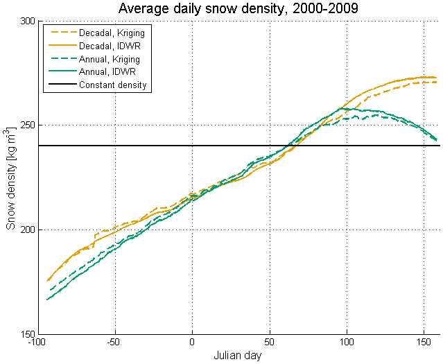
Figure 3 Average daily snow density between 2000–2009 for four different snow density versions. The constant snow density used in SWE retrieval procedure is also shown.

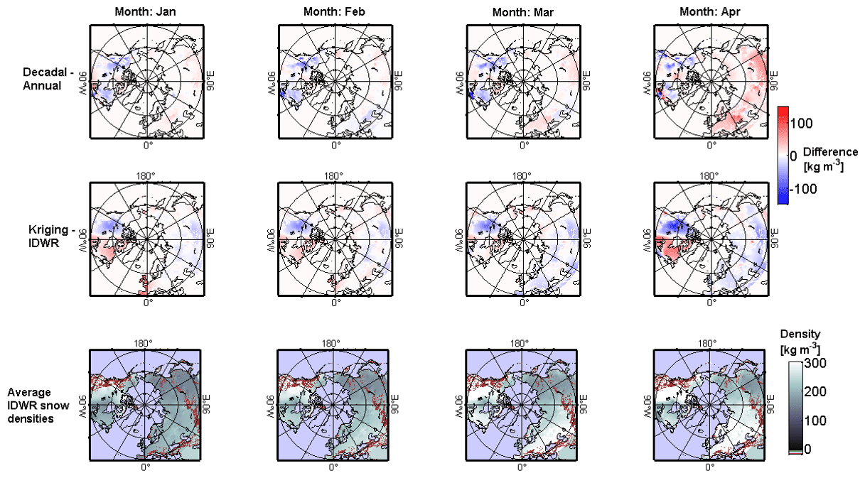
Figure 4 Top row shows monthly difference between average snow density values of decadal and annual (Kriging) densities. Middle row shows average differences between Kriging and IDWR (annual) densities. Bottom row shows average IDWR densities. Differences and densities are shown for January, February, March, and April.

Conversely, the decadal densities continue to increase until April when the values stabilize. Analysis of snow densities in Eurasia over 42 years found that snow densities increase throughout the spring (Zhong et al., 2014) in concert with increasing temperatures and snowmelt. However, when looking at shorter time periods or a smaller number of locations, snow density exhibits a more varied behaviour. Specifically, although snow densities generally increase over the course of the snow season, often times there is a reduction in density at the end of the season before the full snow cover has ablated (see, for example, Bormann et al., 2013). Figure 4 shows differences in monthly average densities between two Kriging-interpolated density sets (decadal and annual) and between two annual (Kriging and IDWR) sets of densities, as well as the monthly average IDWR densities for January, February, March, and April. Annual Kriging-interpolated densities are generally higher than decadal Kriging densities in North America. In Eurasia, differences are small between annual and decadal densities, except in April when decadal densities are higher, which is consistent with Fig. 3. IDWR densities are consistently higher in western North America and lower in eastern North America compared to the annual Kriging-interpolated values. IDWR densities are also usually higher in Eurasia, except western Europe in January and February, than the Kriging densities. In North America, there is a clear delineation between east and west in the IDWR density field (bottom row of Fig. 4) that is not present in Kriging-interpolated densities. This feature is most likely due to the dense network of automated snow measurements in the western United States. These measurements have a more significant effect on IDWR densities than on the Kriging-interpolated densities, as only one variogram is fitted for North America.

4.2 Dynamic snow densities inside the SWE retrieval

As outlined in Sect. 2, snow density is an input to the HUT snow emission model that is used to estimate effective snow grain size at locations with in situ SD measurements and to model the brightness temperature. Snow density is also used to convert the final SD estimate to SWE. To understand the effect of implementing dynamic snow densities into the SWE retrieval more clearly, we look at the impact of dynamic snow densities on (i) effective snow grain size (Sect. 5.2.1) and (ii) SWE estimates made without constraining the retrieval with the background SD field in step 4 (Sect. 5.2.2). For these two analyses, we compare the IDWR version, which had the best snow density accuracy (Sect. 5.1), to GlobSnow 3.0 (static density) for a test year (2005). The year 2005 was chosen as a test year as the performance of the GlobSnow SWE retrieval is average that year. Additionally, the behaviour and amount of snow mass is similar to the 10-year average in 2005. We then assess the impact of dynamic density on the final SWE retrieval (Sect. 5.2.3), outlined in Sect. 2, in comparison to the baseline GlobSnow v3.0 dataset and a dataset where variable densities are implemented in post-processing.

4.2.1 Effective snow grain size

The effective snow grain size, d₀, is that which minimizes the error in modelled T_b compared to the satellite observations, and it is used to compensate for spatial and temporal changes in the snow structure. In the SWE retrieval procedure, the d₀ values range between 0.2 and 2.5 mm. Values smaller than 0.2 mm are rounded up to 0.2 mm, while values larger than 2.5 mm do not occur as this is the upper limit set in step 2 in the inversion of the HUT snow model. Figure 5 shows the monthly average effective snow grain sizes for January, February, March, and April 2005 for the GSv3.0 product and the product with the annual IDWR snow densities implemented into the SWE retrieval. Figure 5 also shows differences in average d₀ between the two products for the 4 months under investigation. Figure 6 shows distributions of d₀ values for January, February, March, and April 2005 for GSv.3.0 and IDWR products. We have focused our analysis on the product with IDWR densities implemented into the processor, as IDWR densities have the best overall performance of the four different density versions.

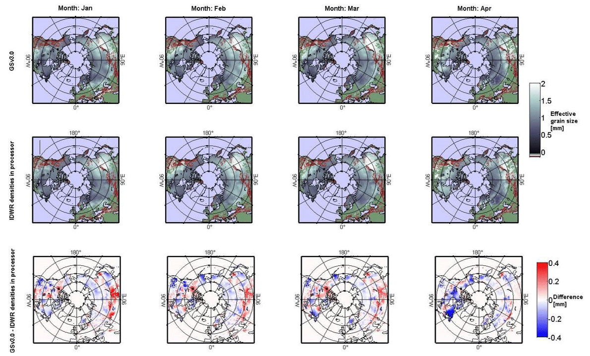
Figure 5 Monthly average effective snow grain sizes for GSv3.0 and IDWR densities in the SWE processor are shown in the top and middle row, respectively. Effective snow grain sizes are shown for January, February, March, and April 2005. Bottom row shows the differences in average effective snow grain sizes between GSv3.0 and IDWR densities in the processor.

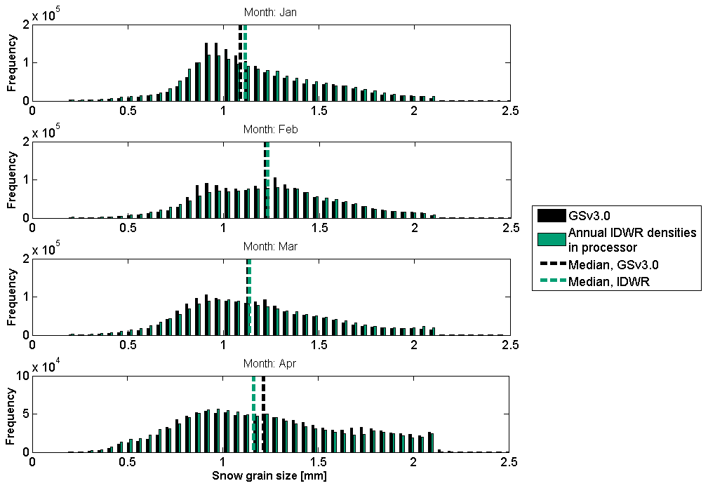
Figure 6 Histograms of effective snow grain size values for January, February, March, and April 2005. The monthly median value is shown with dotted lines.

The effective snow grain size is affected by multiple factors that include snow microstructure and variations in land cover, soil, and vegetation. IDWR grain sizes tend to be larger in northern Eurasia and eastern North America through the winter and smaller in central Eurasia and northwest North America compared to the GSv3.0 grain sizes. Overall, for January, February, and March, IDWR effective snow grain size values are larger than those of GSv3.0. The monthly mean d₀ values show how the effective grain size values grow from January to February but are smallest in March and slightly larger in April.

Although there are some large (local) differences in snow grain size estimates between the density implementations, these changes do not necessarily correspond to large differences in snow density (between static density and IDWR densities) and vice versa. Differences in grain size (between constant and dynamic density implementations; Fig. 5) are smaller than the differences in density themselves. This is not surprising given that snow density is only one of multiple parameters ingested by the HUT emission model. The passive microwave brightness information is the same in both the constant and dynamic density implementations, so slightly altering the snow density while keeping all other parameters the same will not yield substantial changes in grain size, which in the retrieval algorithm essentially acts as a fitting parameter to achieve optimal agreement between simulated and observed T_b. Furthermore, the final effective snow grain size estimate (and its variance) at each location is the average grain size of the six nearest stations, which produces a smoother field than that of SD or density. Snow density influences not only the grain size estimates themselves but also the magnitude of the variance, which in turn affects the weight of the radiometer data on the final SWE estimation (left-hand side of Eq. 1). If the true snow density between stations varies significantly, the variance of the estimated snow grain sizes increases. Higher variances are often associated with less accurate individual grain size estimates and can potentially reduce the weight of radiometer measurements on the final SWE estimation. Using dynamic snow densities can help with this, as these varying snow densities are likely to be closer to the true snow density at each location compared to the constant density, thereby improving effective grain size estimates.

4.2.2 SWE retrieval without the final assimilation

To isolate the effect of implementing dynamic snow densities inside the SWE retrieval, we ran the retrieval without constraining it with the background SD field in step 4. That is to say that the SWE estimates are made without the final SD assimilation by minimizing the difference between modelled and measured T_b observations (i.e. only the left-hand side of Eq. 1 was run). The background SD field can have a considerable impact on the final SWE estimates, and it can dampen the effects of other input data and parameterizations such as snow density. Running the SWE retrieval without the final SD assimilation helps to highlight the effects of dynamic snow densities on the SWE retrieval. Synoptic SD observations are still used to estimate effective snow grain size at the measurement station locations (step 2). We again focus our analysis on the product produced using annual IDWR densities.

Figure 7 shows density scatter plots and validation parameters for SWE retrievals without the final SD assimilation with static and annual IDWR densities for the year 2005. Validation parameters are calculated using the validation datasets (Fig. 1, blue). As seen in Fig. 4, MAE and bias are smaller for the IDWR density version than for the static density version, but the RMSE is larger. The scatter plots show that the IDWR version has a large concentration of points following the diagonal line but also more outlier values than the static snow density product. This concentration of points, which are located in eastern Russia (around 120^∘ E), explains the smaller MAE and bias and larger RMSE (RMSE is more sensitive to outliers than MAE) of the IDWR density version as compared to the static density product. It is promising that the annual IDWR densities are able to produce improved SWE estimates when compared to the static density product even when the retrieval is not constrained with the background SD field. In the next section we will look at the full retrieval.

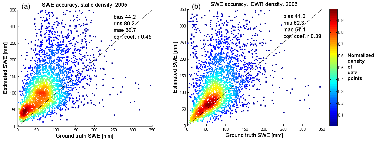
Figure 7 Scatter plots showing the normalized density of scattered points and validation parameters for SWE retrievals without final assimilation with static density (a) and IDWR-interpolated dynamic density (b) for 2005.

4.2.3 SWE retrieval results

Finally, we ran the full processing algorithm, including the final SD assimilation step, for each of the four dynamic density versions. The SWE retrieval results from each of the four dynamic density versions are compared with the baseline GSv3.0 dataset and a post-processed dataset. The post-processed product is similar to that of Venäläinen et al. (2021) but with updated snow density data consistent with those used in this study. The validation parameters shown in Table 3 are again calculated using the validation dataset (Fig. 1, blue).

Table 3 Summary of validation parameters for GSv3.0, post-processed product, and different densities in the retrieval products for 2000–2009 for SWE < $\mathrm{500}/\mathrm{200}$ mm. The best value in each category is in bold.

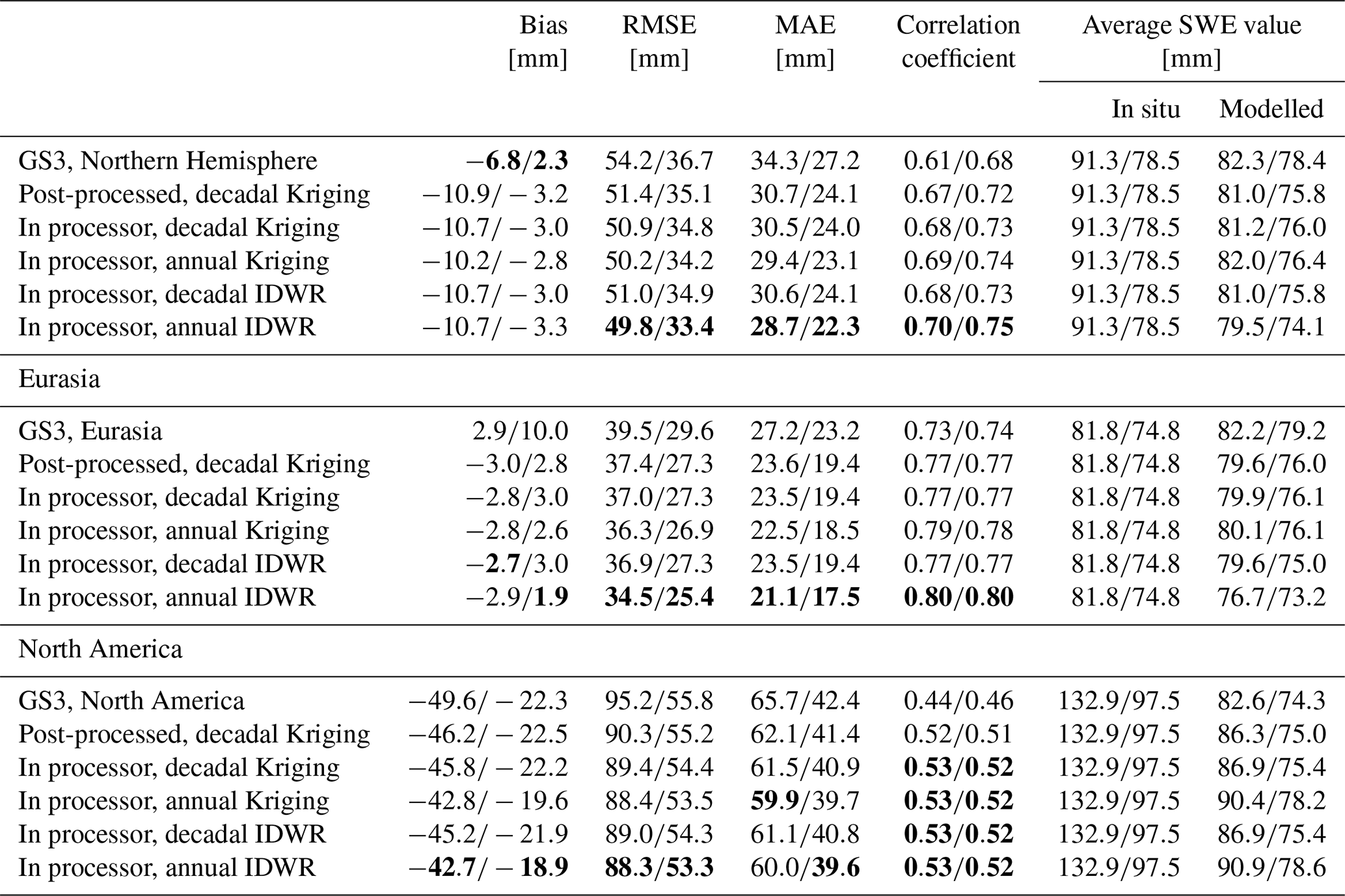
As shown in Table 3, both adjusting the SWE retrieval with dynamic snow densities in post-processing and inserting dynamic snow densities into the retrieval improve RMSE, MAE, and correlation when compared to the baseline GSv3.0 product. This shows that spatially and temporally varying snow densities provide a more accurate SWE estimate than a single constant value does. Furthermore, applying dynamic density inside the algorithm produces more accurate SWE retrievals than applying it in post-processing. Overall, IDWR interpolation performs better than Kriging interpolation, which is consistent with the results from Sect. 5.1 that showed IDWR had the most accurate snow density accuracies for Eurasia and the most accurate annual snow densities in North America. In general, annual densities yield more accurate SWE retrievals than decadal densities when implemented into the retrieval. This result differs slightly from our analysis of the density fields (Sect. 5.1) which found the decadal version to have the best accuracies over North America. Although the decadal densities had better RMSE and correlations in North America (especially in western North America), from January onwards, decadal density values are consistently lower than the annual densities (Sect. 5.1). For the same SD, lower snow densities result in lower SWE (retrieve SD is converted to SWE using snow density value); these smaller decadal densities may explain the poorer SWE estimates obtained with the decadal densities (compared to annual) in North America where SWE is generally underestimated in middle to late winter. The lower SWE values obtained with the decadal densities will therefore be less accurate.

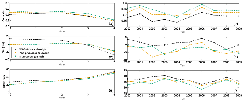
Figure 8 Correlation, bias, and RMSE by month (a, c, e) and year (b, d, f) against validation data.

Figure 8 shows monthly and annual bias, correlation coefficient, and RMSE against validation data for the Northern Hemisphere for 2000–2009 for the GSv3.0 product, decadal post-processed product, and product with annual IDWR densities implemented into the retrieval. Similar to Table 3, we see that post-processing and implementing densities into the retrieval improve SWE estimates when compared to the GSv3.0 dataset. IDWR densities reduce the overestimation (underestimation) at low (high) SWE values compared to the post-processed and baseline (GSv3) versions. Accuracy differences between density versions implemented inside the processor are small compared to the difference from implementing dynamic densities inside the algorithm rather than in post-processing. Overall, the choice of dynamic density field (annual/decadal or IDWR/Kriging) and the way it is applied to estimate SWE (inside the processor or post-processing) have a much smaller impact than the choice of a constant density value versus a variable snow density value does. It is encouraging, though not surprising, that more accurate local densities yield improved SWE retrievals.

4.3 Northern Hemisphere snow mass

Figure 9 shows the total average snow mass for the Northern Hemisphere (excluding mountains) for 2000–2009 for the GSv3.0 product, decadal Kriging post-processed product, and the product with the annul IDWR densities implemented into the retrieval. Both post-processing and implementing densities into the retrieval shift the timing of peak snow mass later, bringing it more in line with gridded reanalysis products and historically forced snow models (Mortimer et al., 2022), but post-processing reduces the snow mass when compared to the GSv3.0 dataset which is already biased low (Pulliainen et al., 2020). When dynamic snow densities are implemented into the retrieval, the aforementioned reduction in snow mass is negligible. The IDWR approach retains the magnitude of peak SWE present in GSv3 and the timing of peak SWE of the post-processed version.

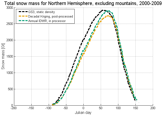
Figure 9 The total Northern Hemisphere snow mass (without mountains) calculated from GSv3.0 and dynamic densities in retrieval products for 2000–2009.

Figure 10 shows spatial differences in average monthly SWE (for a 10-year period from 2000–2009) between the decadal Kriging post-processed SWE product and GSv3.0 product (top row), the differences between the product with dynamic annual IDWR densities in retrieval and the GSv3.0 product (middle row), and differences between the decadal Kriging post-processed product and the product with dynamic annual IDWR densities in retrieval (bottom row).

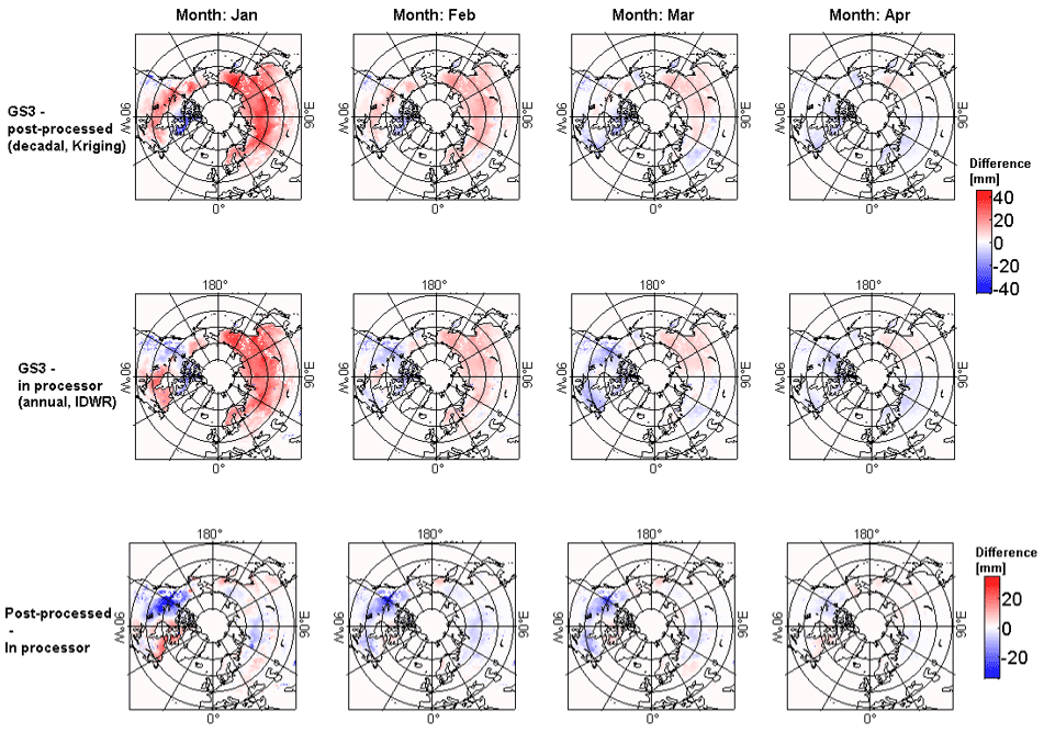
Figure 10 Top row shows the average monthly difference in SWE between the GSv3.0 product and post-processed product (decadal, Kriging). The middle row shows the average monthly difference between the GSv3.0 product and product with IDWR densities inside the processor. The bottom row shows the average monthly difference between the post-processed product and product with IDWR densities in the processor. Note the differing scales in the monthly (left) and annual (right) plots. Monthly averages are calculated for the years 2000–2009.

Over the course of the snow season, the GlobSnow v3.0 SWE bias generally follows the degree of over-/underestimation of the constant density compared to the true snow density (Mortimer et al., 2022). In early winter, the constant density of 240 kg m⁻³ is often too high (Fig. 3 shows that the daily average snow density value of all dynamic snow density versions reaches the constant density in mid-March), and the retrieval overestimates at the lower ranges of SWE (e.g. below ∼100 mm; see Fig. 8). Overall differences between different products are smaller in Eurasia than in North America, and the largest differences occur in January (earlier months in the snow season not shown) and decrease as the snow season progresses. Spatially, GSv3.0 has higher SWE than the dynamic density products (post-processed and inside the retrieval) for large parts of Eurasia throughout the year, except for western Europe in March and April as indicated by the red colours in Fig. 10. Both post-processing and implementing densities into the retrieval reduce much of this overestimation in Eurasia, but differences are slightly more muted when dynamic densities are implemented inside the processor (compared to in post-processing).

The magnitude and spatial distribution of SWE differences compared to GSv3.0 with the post-processed and inside retrieval density implementations are more varied in North America compared to Eurasia. In North America, post-processing reduced SWE in January and February across the boreal forest and increased it in the Canadian Arctic Archipelago (CAA) and coastal western US. Conversely, when dynamic densities are implemented inside the retrieval, January SWE is lower (compared to GSv3.0) in eastern Canada and parts of Alaska and higher in the west (west of ∼100^∘ W) and the CAA. The spatial pattern of January SWE between GSv3.0 and IDWR somewhat mirrors the density pattern in Fig. 4 where IDWR densities were lower (higher) east (west) of 100^∘ W compared to Kriging densities. In January the post-processed product has larger (smaller) SWE values in eastern (western) North America than the version with IDWR densities implemented in the processor. In February, IDWR SWE is generally higher than GSv3.0 except in central Canada south of Hudson Bay and in Alaska. In March and April, both density implementations result in higher SWE across North America (with some exceptions), and the magnitude of increased SWE compared to GSv3.0 is larger when densities are implemented inside the retrieval. North America tends to have higher SWE than Eurasia, so seeing a larger increase in SWE in the IDWR product compared to GlobSnow is encouraging, although not unexpected.

5 Discussion

A key limitation of passive microwave SWE retrievals is the systematic underestimation of large SWE values and overestimation of small SWE values. Most passive microwave SWE retrieval algorithms are based on differences between measurements made at a frequency sensitive to snow grain volume scattering and measurements at a frequency considered largely insensitive to snow (Chang et al., 1987; Kelly, 2009; Tedesco and Narvekar, 2010). This leads to the underestimation of SWE values under deep-snow conditions (larger than 150 mm) as the snowpack changes from a scattering medium to a source of emission. The GlobSnow SWE algorithm partially mitigates this issue with the assimilation of in situ snow depth measurements and provides better estimates for moderate snowpacks (SWE ∼ <200 mm) than stand-alone passive microwave algorithms (Mortimer et al., 2020). However, the underestimation (overestimation) of large (small) SWE values is still present in the GlobSnow retrieval. One key remaining source of uncertainty in the GlobSnow SWE retrieval is the use of a constant snow density with value of 240 kg m⁻³. Although this is a reasonable mean value, it fails to capture spatial and temporal density variability, which in turn can lead to local inaccuracies. Snow density is one of the input parameters to the HUT snow emission model which determines the absorption coefficient of snow, refraction, transmissivity at the snow–ground interface, and transmissivity at the air–snow interface through modelled permittivity of the snow layer (Pulliainen et al., 1999). The HUT snow model is used within the retrieval algorithm to ascertain d₀ estimates at weather station locations (step 2) and to determine the final SWE estimates using numerical model inversion (step 4). More accurate snow density estimates can improve effective snow grain size estimates (and decrease variance), as well as the modelled T_b estimates used to determine the final SWE estimates. Additionally, snow density values are used to convert retrieved snow depth to SWE (step 4), and the constant density used in the GSv3.0 is often too small (large) in late (early) winter, which decreases (increases) SWE estimates. This final step of converting retrieved SD values to SWE values can be improved by using dynamic snow densities in post-processing, but it has been found to reduce the total snow mass. When dynamic densities are implemented inside the retrieval, retrieved SD values are improved, and after conversion to SWE, the reduction in Northern Hemisphere snow mass compared to GSv3.0 is negligible.

SWE retrieval without constraining the retrieval with the background SD (Sect. 5.2.2) helps to isolate the impact of dynamic snow densities on SWE retrieval. The background SD field can have a substantial impact on the final SWE estimates, and it can dampen the effects of other input data and parameterizations such as snow density. Without the assimilation of SD, using dynamic densities inside the retrieval produced a smaller MAE but larger RMSE than using the constant density. We attribute the larger RMSE, when dynamic densities are used, to the presence of outlier values (Fig. 7) concentrated in a small area of eastern Russia. However, Fig. 7 shows that the bulk of the SWE estimates made using varying densities are improved compared to static snow density estimates; specifically, the largest density of points more closely follows the 1:1 line. When the retrieval is constrained with the background SD field, these outlier values are removed, and the dynamic density product has a smaller RMSE than the static density SWE retrieval. Outliers are reduced or removed when the background SD field is used because, when the HUT model T_b estimates are matched to T_b observations by incrementing the SD values (step 4), the procedure is constrained with the background SD field, and more optimal SD estimates are obtained than when this step is not constrained. For comparison, when the SWE retrieval is constrained with the background SD field, the RMSE is 46.03 and 42.11 mm and MAE 31.40 and 26.30 mm for GSv3.0 and IDWR densities in retrieval, respectively, for the same period as shown in Fig. 4 (i.e. year 2005). Using the background SD field, which is a key feature of the GlobSnow algorithm, improves RMSE by around 40 mm and MAE by around 30 mm regardless of the density parameterization.

It is well documented that the GlobSnow SWE retrieval algorithm performs better in Eurasia than in North America (Mortimer et al., 2020, 2022). The weaker retrieval skill over North America is partially due to higher average SWE in North America. As seen in Table 2, the average measured SWE is 132.9 mm in North America compared to 81.8 mm in Eurasia. Locations with a high RMSE tend to have a large negative bias and generally correspond to locations with higher SWE. As seen in Fig. 8, RMSE increases and correlation decreases as the bias becomes more negative. Snow densities are larger in North America (274.0 kg m⁻³ in North America and 216.7 kg m⁻³ in Eurasia) and are farther from the static value (240.0 kg m⁻³). Therefore, we might have expected larger improvements in North America (compared to Eurasia) when moving from a constant to a variable density. However, although accuracies improved in both domains, the magnitude of improvement was larger in Eurasia (12.6 % and 14.2 %) compared to North America (7.2 % and 4.5 %) (<500 and 200 mm).

In North America, large errors occur in densely forested high-SWE areas in the northeast and in the mountainous west (Mortimer et al., 2022; Fig. 7). Dense forest and high SWE are challenging for stand-alone passive microwave SWE retrievals. Assimilation of in situ SD information from a sufficiently dense observation network can improve SWE estimates in forested deep-snow regions such as Finland (Pulliainen, 2006; Takala et al., 2011). However, if the in situ SD network is sparse and the SD variance high, as is the case in northern Quebec, Canada, the SWE estimate is more heavily weighted towards the passive microwave information, which has limited sensitivity to higher SWE (Larue et al., 2017; Brown et al., 2018). Complex terrain is masked out in GlobSnow, but high mountain plateaus, which often have high SWE, are included and can result in large errors in parts of western North America.

While developing and evaluating the density fields to be implemented into the retrieval algorithm, we found the IDWR interpolation produced more accurate density estimates than (annual) Kriging interpolation. Similarly, implementing annual IDWR densities into the SWE retrieval resulted in larger improvements compared to the Kriging densities. Differences between IDWR and Kriging were larger in Eurasia than in North America. In North America, available snow density measurements are clustered (Fig. 1), meaning validation locations are often quite close to implementation locations. In Eurasia, the in situ data are more distributed across the region, resulting in greater distances between validation and implementation locations. This different spatial distribution of available snow density data may also explain some of the differences in performance between North America and Eurasia as the IDWR interpolation is known to produce better results than Kriging interpolation when the amount of data is limited (Sect. 4.2). Additionally, the fitting the variogram is an important part of Kriging interpolation, and if the variogram does not adequately describe the data, Kriging may not provide optimal predictive results. When calculating dynamic snow densities using Kriging interpolation, the variogram is fitted daily for two separate areas: North America and Eurasia. This means that small-scale local behaviour of the snow density might not be reflected in the Kriged density fields. The IDWR interpolation captures more local variability, which can have both positive and negative consequences. For example, although IDWR density estimates are more accurate than Kriging-interpolated densities in North America, there is an artificial border in the IDWR density estimates between eastern and western North America that is not present in the Kriging-interpolated densities.

At the hemispheric scale, using annual snow densities (Kriging and IDWR) in SWE retrieval was found to produce better results than using decadal snow densities. However, one issue connected with the use of annual densities is the availability of snow density data. In many cases, snow transect data only become publicly available after a significant delay. Hence, if the goal is to produce near-real-time SWE retrievals, historical snow density data need to be used. For these purposes, decadal or model-based snow densities are required. Another approach for obtaining dynamic snow density information would be to use snow density information available from different reanalysis products. For example, snow density data from ERA5-land were successfully used as an input to the HUT snow model in a study by Yang et al. (2021). We have not used reanalysis products in the GlobSnow SWE retrieval to keep the retrieval independent of reanalysis products and dependent only on observed data.

6 Conclusion

In this study, we implemented three different versions of spatially and temporally varying snow densities into the GlobSnow SWE retrieval methodology in place of a constant density value with the goal of improving SWE retrieval. The first two snow density versions use Kriging interpolation – one with decadal data (10-year daily average snow densities) and the other with annual data (daily average snow densities or just single measurements). These two versions allowed us to test the impact of temporal aggregation and interpolation approaches. The third version uses annual data and IDWR interpolation and allowed us to evaluate effects of different spatial interpolation methods. Annual IDWR densities had the most accurate snow densities in Eurasia and were superior to the annual Kriging densities in North America. However, in North America, the most accurate interpolated densities were obtained using decadal data with Kriging interpolation. Implementing varying snow densities into SWE retrieval altered effective snow grain size estimates when compared to the baseline GSv3.0 grain size estimates. Although differences in effective snow grain size estimates over the full Northern Hemisphere domain were quite small, there were large local differences. Differences in grain size (between constant and dynamic density implementations) are smaller than the differences in snow densities and can be explained by the fact that density is only one of multiple parameters ingested by the HUT emission model and that the effective grain size is essentially a fitting parameter to optimize agreement between simulated and observed T_b.

We found that implementing these dynamic snow densities into the SWE retrieval algorithm improved the accuracy of the retrieval. Snow densities implemented using annual data and IDWR spatial interpolation produced the best results, reducing the RMSE and MAE by about 8 % (9 %) and 16 % (18 %), respectively, for SWE under 500 (200) mm. Implementing varying densities into the retrieval reduced the overestimation of small SWE values and the underestimation of large SWE values, though the underestimation of large SWE values is still present. The assimilation of SD data used in the GlobSnow retrieval improves estimates of large SWE values when compared to algorithms based only on radiometer data. However, the physics upon which the SWE retrieval is based limits the SWE estimates to below about 200 mm. Similar improvements in validation parameters (RMSE, MAE, and correlation coefficient) are obtained when the baseline SWE product is post-processed with the dynamic snow densities. However, post-processing reduced the total Northern Hemisphere snow mass when compared to GSv3.0, which itself is biased low. Implementing dynamic snow densities into the SWE retrieval removes this reduction in the Northern Hemisphere peak snow mass. Additionally, both implementing dynamic snow densities into the SWE retrieval and using them for post-processing delay the timing of the peak snow mass by around 2 weeks, which brings it more in line with other hemispheric SWE datasets (Mortimer et al., 2022). The development of the SWE retrieval algorithm continues in the ESA SnowCCI+ project, and, as implementing annual dynamic snow densities into the retrieval improves the retrieval skill, this modification will be used in the production of the next iteration of ESA SnowCCI+ SWE. However, as decadal snow densities are more accurate in North America, they might be preferred for some applications.

Appendix A: Validation of snow densities in North America

Table A1 Validation parameters of different snow densities for eastern (east of 90^∘ W) and western North America.