the Creative Commons Attribution 4.0 License.
the Creative Commons Attribution 4.0 License.
 | 09 Feb 2023
The benefits of homogenising snow depth series – Impacts on decadal trends and extremes for Switzerland
Moritz Buchmann
Gernot Resch
Michael Begert
Stefan Brönnimann
Barbara Chimani
Wolfgang Schöner
Christoph Marty
Our current knowledge of spatial and temporal snow depth trends is based almost exclusively on time series of non-homogenised observational data. However, like other long-term series from observations, they are prone to inhomogeneities that can influence and even change trends if not taken into account. In order to assess the relevance of homogenisation for time-series analysis of daily snow depths, we investigated the effects of adjusting inhomogeneities in the extensive network of Swiss snow depth observations for trends and changes in extreme values of commonly used snow indices, such as snow days, seasonal averages or maximum snow depths in the period 1961–2021. Three homogenisation methods were compared for this task: Climatol and HOMER, which apply median-based adjustments, and the quantile-based interpQM. All three were run using the same input data with identical break points. We found that they agree well on trends of seasonal average snow depth, while differences are detectable for seasonal maxima and the corresponding extreme values. Differences between homogenised and non-homogenised series result mainly from the approach for generating reference series. The comparison of homogenised and original values for the 50-year return level of seasonal maximum snow depth showed that the quantile-based method had the smallest number of stations outside the 95 % confidence interval. Using a multiple-criteria approach, e.g. thresholds for series correlation (>0.7) as well as for vertical (<300 m) and horizontal (<100 km) distances, proved to be better suited than using correlation or distances alone. Overall, the homogenisation of snow depth series changed all positive trends for derived series of snow days to either no trend or negative trends and amplifying the negative mean trend, especially for stations >1500 m. The number of stations with a significant negative trend increased between 7 % and 21 % depending on the method, with the strongest changes occurring at high snow depths. The reduction in the 95 % confidence intervals of the absolute maximum snow depth of each station indicates a decrease in variation and an increase in confidence in the results.
- Article
(5182 KB) - Full-text XML
- BibTeX
- EndNote


During winter in the Northern Hemisphere, more than 50 % of the earth's surface can be covered with snow (Armstrong and Brun, 2008). The thickness and duration of a snow cover play an important role for many animal and plant species (Johnston et al., 2019) but also have an important socio-economic dimension: for example, the timing and amount of snowmelt are important for hydropower companies, and the number of days with a certain minimum snow depth (e.g. 30 cm) is a metric widely used for the profitability of ski resorts (Abegg et al., 2020). Accurate and reliable measurements of solid precipitation, e.g. total height of fallen snow (snow depth) or the amount of freshly fallen snow (depth of snowfall), are difficult to obtain but are important (Nitu et al., 2018) as they are used for various purposes, e.g. as ground evidence for large-scale grid-based forecasts of snow depth (Olefs et al., 2013) or the operational assessment of snow models used for avalanche hazard forecasting (Morin et al., 2020). Long-term measurements are key to climate monitoring and related analyses. They are not only used for climatological analyses (Matiu et al., 2021; Pulliainen et al., 2020), but also for creating bias-corrected models (Maraun et al., 2017) and gridded data sets (Cornes et al., 2018; Hiebl and Frei, 2018; Hersbach et al., 2020; Li et al., 2022).
All climate time series comprise a climate signal, a station signal and white noise (Caussinus and Mestre, 2004). The station signal includes the characteristics of the environment, observers and instruments of each station. If the station signal changes over time, it can alter the climate signal, e.g. by amplifying or weakening trends. It should therefore be adjusted before further analysis is done. According to the approach of relative homogeneity testing and adjusting, this is possible as long as neighbouring stations follow an identical climatic signal (variability and trend). The longer the time series, the higher the probability of large changes causing breaks/break points in it. There are many reasons for this, such as changes in instruments, observers, the station environment, or a combination of the above factors (Auer et al., 2007; Venema et al., 2020). Alexandersson and Moberg (1997) even found that multi-decadal time series without breaks are rare. Breaks can significantly alter derived trends (Begert et al., 2005; Gubler et al., 2017; Resch et al., 2022) and extreme values (Kuglitsch et al., 2009). Therefore, to address this problem, climate time series should be homogenised, which does not always happen or is not always possible, usually by a two-step procedure. First, immanent break points are identified. Relative homogeneity tests used for break point identification mostly assess significant changes in ratios or differences between the station to be homogenised (candidate series) and neighbouring stations (reference series). Reference series are selected on the basis of several criteria, mostly correlation and horizontal as well as vertical distance. In a second step, the candidate series is homogenised to the present state, thus compensating for previous non-climatic deviations, e.g. changes in observation procedures, sensors or measurement techniques, in the time series.
Today, this is a standard procedure for climate data like temperature and precipitation (Venema et al., 2020) but has only recently been adopted for snow depth time series: the first steps towards detecting and adjusting breaks were made by Marcolini et al. (2017). Schöner et al. (2019) used the HOMOP tool (Nemec et al., 2013) to homogenise seasonal depth time series and to calculate trends and identify snow regions in Austria and Switzerland. Marcolini et al. (2019) compared the performance of two homogenisation methods (HOMOP and SNHT; Alexandersson, 1986; Alexandersson and Moberg, 1997) and their effects on trends in seasonal mean snow depth. Their results showed the need to improve adjustment methods in order to (i) enable the application to data with higher temporal resolution (e.g. daily data) and (ii) to improve the adjustment of extreme values. Taking up these needs, an adjustment method using quantile matching was introduced by Resch et al. (2022).
Widely used metrics to describe the snow cover include average and maximum snow depths and days with a snow depth above a certain threshold, referred to here as snow days. This commonly used index is defined as the number of days within a certain time period (e.g. season) with a certain snow depth, usually between 1 and 50 cm (Abegg et al., 2020; Schmucki et al., 2017). Snow days are relevant for ecology (Stone et al., 2002; Jonas et al., 2008), climatology (Scherrer et al., 2004; Marty, 2008) or the ski tourism industry (Abegg et al., 2020), whereas the average and maximum snow depths are particularly applicable to climatology and engineering applications. Trend and extreme value analyses of snow indices (Scherrer et al., 2013; Matiu et al., 2021) are common methods in climate monitoring (Bocchiola et al., 2008; Marty and Blanchet, 2012; Buchmann et al., 2021a) and model verification (Brown et al., 2003; Essery et al., 2013), while extreme value analyses are important for defining snow loads and limits for building codes (Croce et al., 2021; Schellander et al., 2021; Al-Rubaye et al., 2022).
We use the break points recently identified by Buchmann et al. (2022b) for manual Swiss snow series with a joint application of three widely used break point detection and homogenisation methods, ACMANT (Domonkos, 2011), Climatol (Guijarro, 2018) and HOMER (Mestre et al., 2013), for three homogenisation methods to calculate and apply adjustments: Climatol, HOMER and interpQM (Resch et al., 2022). ACMANT, which is fully automatic, does not allow manual break point input and was therefore not used for our analyses. The first two methods apply median-based adjustments, and the latter uses a quantile-based approach. All three methods are then applied to the network of Swiss snow depth time series. This allows us to assess the impact of homogenisation (dependent on the method used) on the trends in seasonal mean and maximum snow depths, days with snow on the ground and extreme values of maximum snow depths.
Our research questions are the following.
-
How do the homogenised series compare across the three methods used?
-
What influence does homogenisation have on the decadal trends in average and maximum snow depth?
-
How do the three homogenisation methods affect widely used snow indices?
-
To what extent are the maximum snow depths with a 50-year return period (as an example of snow metrics used by practitioners) affected by the different homogenisation methods?
The article is structured as follows. Section 2 describes the data and Sect. 3 introduces the various methods used. Results are shown in Sect. 4 and discussed in Sect. 5. Conclusions are drawn in Sect. 6.
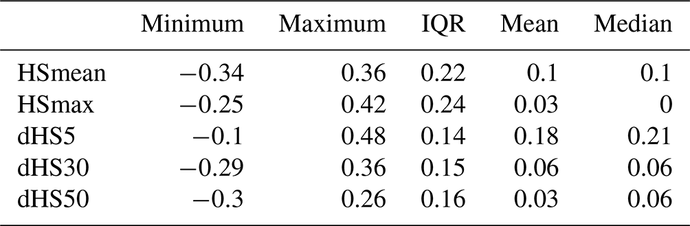
Daily manual snow depth measurements (HS) from 184 Swiss stations serve as the basis for quantifying the benefit of data homogenisation for snow depth series. Seasonal (November to April) and monthly averages (HSavg), maximum snow depths (HSmax), and the number of snow days ≥5 cm (dHS5) are calculated from the daily snow depths measured at 07:00 LT each day. For obvious reasons, daily snow depth time series inherit a strong autocorrelation. We used seasonal indicators of snow depth, which imply no to low autocorrelation with the exception of cases when the snow cover did not completely melt over the summer. However, this is neither the case for any of the selected stations nor for any of the seasons analysed. The autocorrelation was analysed for lags 1–10. The results for lag 1, where it is strongest, are shown in Table 1. The autocorrelation here is very low, with a mean of 0.03–0.18 and an interquartile range of 0.14–0.24. Consequently, a trend-free prewhitening of snow depth series (Yue et al., 2002) or the application of a modified Mann–Kendall (MK) test was not necessary.
Figure 1 shows the station distribution of the 184 Swiss stations used. They are maintained either by the Federal Office of Meteorology and Climatology (MeteoSwiss) or the WSL Institute for Snow and Avalanche Research (SLF), covering the period from 1931 to 2021 and spanning from 200 to 2500 m a.s.l. (shown in the right panel of Fig. 1). Only stations with complete data coverage between November and April for each year and at least 30 years of data are considered. A detailed description of the data set can be found in Buchmann et al. (2022b).
Table 1Summary of autocorrelations for lag (year) 1 for all stations (n=40).
The set of pre-identified break points
We use the set of 45 break points (found in 40 snow depth series) identified by Buchmann et al. (2022b) for our analyses. Two series (stations Bernina Hospiz and Gütsch) were removed from the original 42-station sub-set due to insufficient data quality between 1961 and 2021. Break points were detected using ACMANT (Domonkos, 2011), Climatol (Guijarro, 2018) and HOMER (Mestre et al., 2013), with break points accepted as valid if detected within 2 years by at least two of the three methods. For details, e.g. on the differences between methods in the detected breaks and motivation for the criteria of break acceptance, see Buchmann et al. (2022b). Break points are identified based on seasonal series. Where appropriate, available metadata have been used for verification. However, as our metadata are neither perfect nor complete, they are only used as an additional source of information and not as stand-alone evidence. To improve the station density near the Swiss eastern border, three Austrian stations were added to the database. Figure 1 shows the locations of all 184 Swiss series in the left panel, and stations with detected breaks are marked with pink triangles. The right panel shows the elevation distribution of the stations.
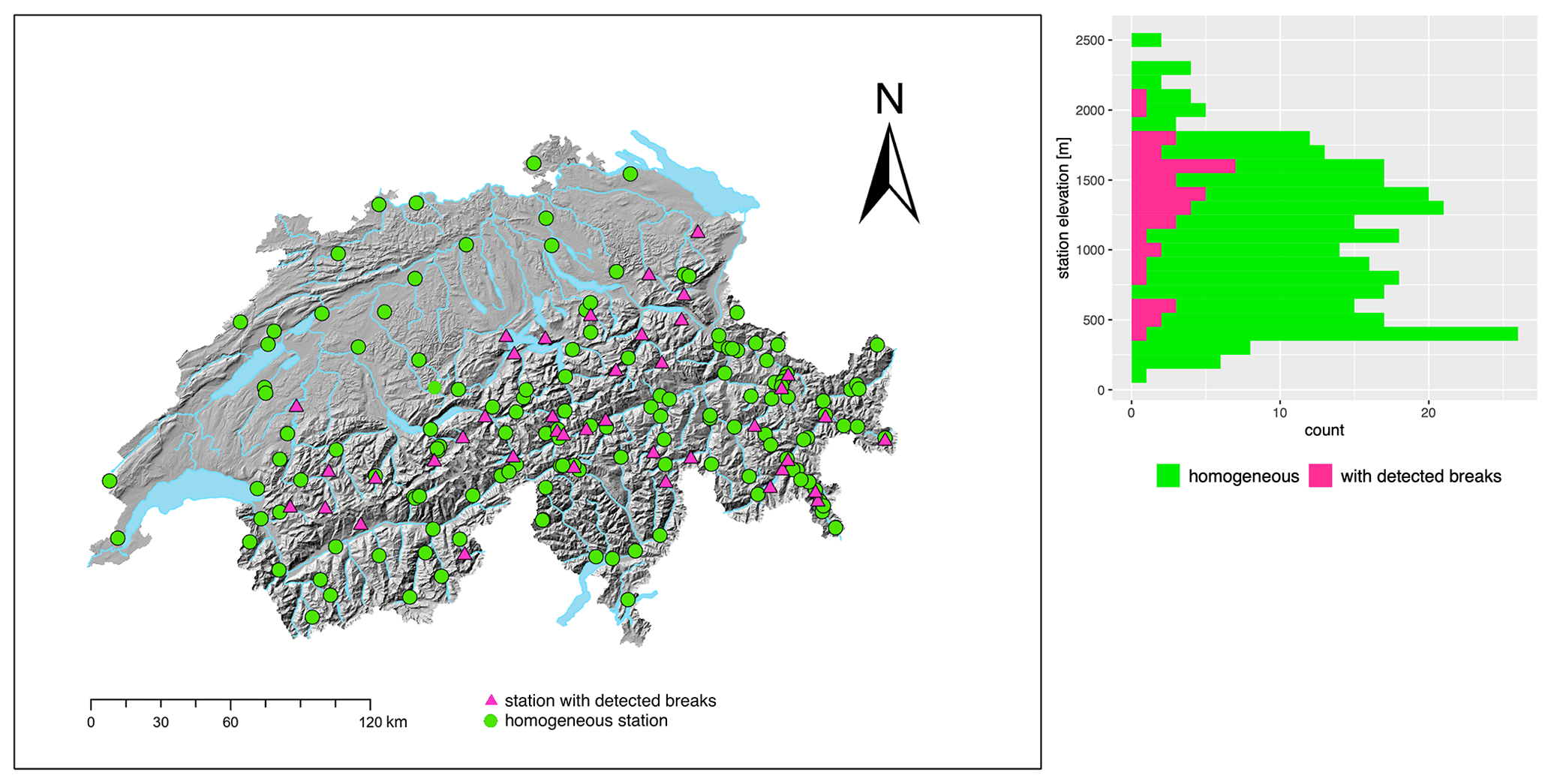
Figure 1Left panel: map of Switzerland with all 184 Swiss stations used in this study. The 40 identified inhomogeneous stations with valid break points are highlighted in pink triangles. The green circles are series that are considered homogeneous. Right panel: elevation distribution of the homogeneous stations and those with detected breaks.
Each break point of a candidate series is adjusted by a multiplicative approach to the most recent status of the snow station. This is in agreement for all three adjustment methods applied. Adjustment factors are based on statistical measures of the candidate and reference series, respectively, and applied to the monthly (Climatol, HOMER) or daily (interpQM) values. These statistical measures (e.g. median, quantiles) applied for adjustment are different for the three methods and are described below. It is important to know that the reference series used for adjustment by the three methods are not identical and are selected on different criteria. For interpQM and HOMER, they are known to the user.
All analysed methods use the same data set to select suitable reference stations for the calculation of the adjustment factors based on the pre-determined break points, which in our case are provided by Buchmann et al. (2022b) and used by each method by importing a file containing the break points. Although it is possible to manually select suitable reference stations for each series and to use only these for each method, we have chosen to let the methods themselves select their reference stations based on their internal criteria.
3.1 Adjustment methods
Climatol (Guijarro, 2018) is a fully automatic homogenisation method based on SNHT (Alexandersson, 1986) for break detection and a linear regression approach following Easterling and Peterson (1995) for the adjustments. It uses composite reference series that are constructed as a weighted average, using the horizontal and vertical distances between a suitable reference and the candidate series as a weight. We used the default settings, i.e. 100 km, where the horizontal distance weight is set to 0.5 and the vertical distance scaling to 0.1. As for all adjustment methods, candidate series are adjusted back in time starting from the most recent homogeneous sub-period. In doing so, each detected break (sub-period between breaks) is adjusted by applying an adjustment factor derived from annual values (see Guijarro, 2018, for details), which is calculated for Climatol as follows.
The adjustment factor of a time series z is calculated as follows:
where and are the mean snow depth between the beginning of the measurements of z and the break point (before) and from the break point to the end (after), respectively. σQ and are the standard deviation and mean of the non-standardised ratio time series (Alexandersson and Moberg, 1997).
HOMER (Mestre et al., 2013) is an interactive semi-automatic toolbox that provides various methods for detection and adjustment of breaks, such as pairwise comparison (Caussinus and Mestre, 2004), a fully automatic detection and correction joint segmentation (Picard et al., 2011) and ACMANT detection (Domonkos, 2011). For our purposes, the pairwise comparison was chosen, as it accepts the use of independently derived break point metadata files like Climatol and interpQM. The series are adjusted with a single annual factor for the entire period before a break point. The adjustment factor is derived from analysis of variance (ANOVA) (Caussinus and Mestre, 2004) based on the selected reference stations. These are defined either on the basis of the horizontal distance or the first-difference correlations. Due to the large vertical distances between stations, even for short horizontal distances, the latter was chosen with a minimum Spearman ρ of >0.8.
where Oij is the matrix of the original time series j with time index i, the estimation of the correction for a set of breaks per candidate station Cj in a homogeneous sub-period hi,j and the estimation of the adjusted station signal with the number of break points of a station kj.
interpQM (Resch et al., 2022) is an extension of INTERP (Vincent et al., 2002), which uses quantile matching to improve the adjustments, taking into account the frequency distribution of the daily values to be adjusted. It provides homogenised data on a daily basis, which then allows the analysis of the subsequently derived snow indicators. For this purpose, the daily measurements of the candidate and reference series are split into two inter-quantile sub-sets (IQSs), which are then compared. An adjustment factor
is calculated for each IQS and then linearly interpolated between neighbouring IQSs to avoid artificial jumps in the data. and are the median of the daily time series of the candidate/reference station before (b) or after (a) the detected break point to be adjusted. The reference series can either be selected manually or be a composite series calculated from a weighted average of selected stations (<100 km horizontal and <300 m vertical distance, >0.7 correlation, no detected breaks), which was chosen here. The selection can be manually refined and optimised using local knowledge and experience. The distribution of weights between these stations can either be exponential or linear. To reduce the strong influence of individual highly correlated stations on the result, a linear distribution of the weighting was chosen. Break points are derived from a pre-defined break point file.
3.2 Detection of trends and changes in snow depth series
The use of homogenisation techniques that adjust daily values allows the analysis of the impact on derived indicators that require daily data for their calculation, e.g. snow days. Only the original data and interpQM are compared here, as HOMER only provides monthly or seasonal data and Climatol kept crashing when using the full daily data set. Since we did not want to pre-select stations as this would influence the results, we decided not to use them for this purpose.
interpQM does not add new days with snow (HS>0). To avoid a possible negative bias and because almost no changes were expected for the homogenised series of days with HS >1 cm, the threshold values of 5, 30 and 50 cm are clearly more meaningful. Snow days are accumulated based on a temporal reference between November and April each year (hydrological year). Trends are determined using the standard non-parametric Mann–Kendall trend test (Mann, 1945; Kendall, 1975) and are considered significant if they are above the 95 % level.
Theil–Sen slopes (Theil, 1950; Sen, 1968) are used to estimate the strength of the trends. The decadal trends are expressed as change in centimetres per decade or days per decade. For the comparison of the homogenised sub-sets of 40 stations, we focus on the period from 1961 to 2021, as most stations have data for this period. The trends for all available decades are provided in the Appendix (Fig. A2).
To investigate the effects of homogenisation on extreme snow depths, return levels for the seasonal maximum snow depth (HSmax) (Marty and Blanchet, 2012) are calculated for a fixed return period of 50 years (Buchmann et al., 2021a; Marty and Blanchet, 2012) based on original and homogenised data (R50HSmax). This approach was chosen because the international standards for maximum snow load on buildings are based on R50HSmax (see e.g. Schellander et al., 2021). The calculations were performed with R package extRemes (Gilleland and Katz, 2016) in default settings (generalized extreme value distribution (GEV), maximum likelihood estimation method (MLE) and 95 % confidence intervals). In order to determine to what extent homogenised and original time series differ in their distribution and to assess the differences between the results of the applied adjustment methods, a two-sample Kolmogorov–Smirnov test (in the following referred to as a KS test) and a non-parametric two-sample Wilcoxon test (in the following referred to as a W test) were performed with seasonal data for all derived indices.
3.3 Intercomparison experiment of adjustment methods
We use the sub-set of 40 stations with identified breaks as input and adjust them with the three methods. While Climatol and HOMER use monthly values as input and thus only provide monthly HSavg and HSmax values, interpQM works with daily snow depth values. From these the analysed seasonal HSavg and HSmax are then derived after the successful adjustment. Decadal trends are calculated for seasonal dHS (snow days) of several thresholds and HSavg aggregated from either monthly HSavg (HOMER and Climatol) or daily HS (interpQM). The largest HSmax value per station, calculated over the entire period (absolute maximum snow depth, maxHSmax), is compared for homogenised and original values. The return levels for seasonal HSmax with a 50-year return period (R50HSmax) are determined either from daily homogenised HS aggregated to seasonal HSmax (interpQM) or from monthly homogenised HSmax (HOMER and Climatol). All calculated trends and the R50HSmax of the different methods are then compared.
Climatol automatically fills in any existing missing dates and interpolates their corresponding values, resulting in an artificially increased length of these series. It also automatically adjusts outliers in the homogeneous period in the default settings.
In the following section, we compare the results of different adjustment methods on the one hand and the homogenised data with the non-homogenised data on the other. In this way we can show both the effect of homogenisation and the dependence of the results on the method used. In Sect. 4.1 we show this as an example for the number of snow days and in particular for the effects on the trend (for interpQM only). Similarly, this is also shown for the maximum snow depth in Sect. 4.2. Finally, in Sect. 4.3 a particular example is given for the magnitude and frequency of extreme snow depth.
4.1 Trends of snow days
Table 2Statistics for snow days (dHS) for the period 1961 to 2021 on a seasonal basis with thresholds of 5 (dHS5), 30 (dHS30) and 50 (dHS50) cm for both original (Orig) and interpQM-homogenised data (iQM).
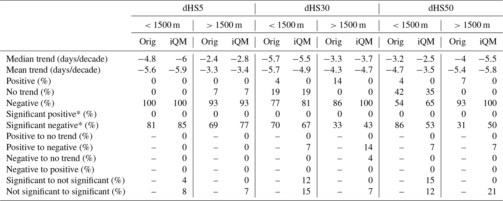
Percentages for significant negative and significant positive, indicated with an asterisk, are calculated based on the total number of negative/positive values, respectively. Positive/negative trends were >0 and <0.
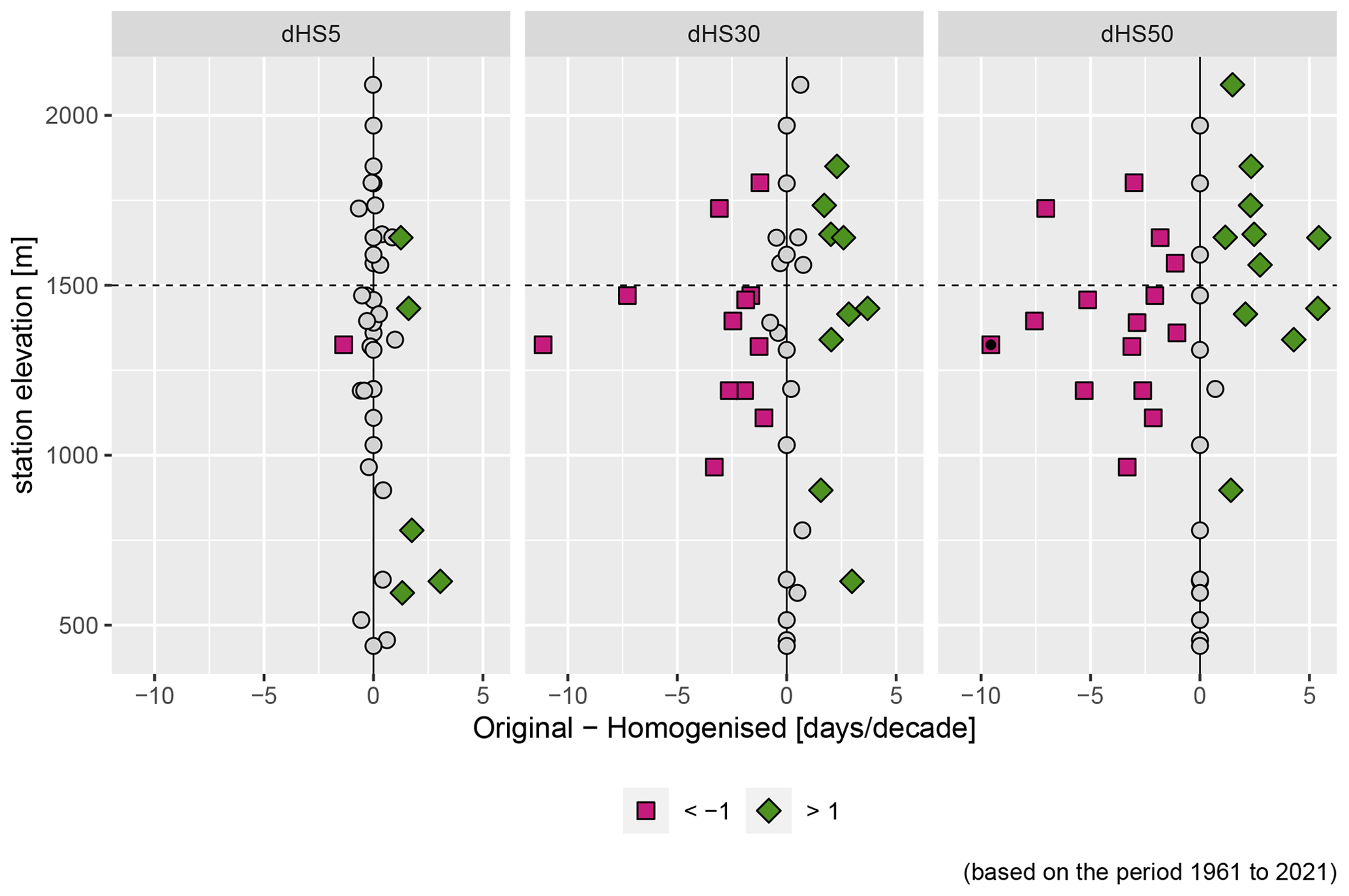
Figure 2Difference in snow day trends between original and interpQM adjusted series for thresholds 5, 30 and 50 cm (dHS5, dHS30 and dHS50). Purple squares indicate stations with a result of , green diamonds >1 d/decade. Black dots indicate a significant difference. Positive values indicate a lower positive or a more strongly negative trend after homogenisation.
The number of snow days per season was examined for two sub-groups of stations, below (n=26) and above (n=14) 1500 m a.s.l., referred to in this section as “low-elevation” and “high-elevation” stations. This threshold was also used by e.g. Auer et al. (2007). Additionally, a strong decrease in snow depth between 1500 and 2500 m was determined for the coming decades (Marke et al., 2015; Marty et al., 2017). This makes this elevation range interesting for analyses of changes that have already taken place. We analysed thresholds of 5, 30 and 50 cm (dHS5, dHS30, dHS50) for the original and homogenised data.
The adjustments made had the strongest effect on dHS30 and dHS50 at stations above 1000 m, as can be seen in Fig. 2. The percentage of significant negative time series increased for all indices above 1500 m and dHS5 below 1500 m, while it was reduced by 3 % for stations below 1500 m for dHS30 and by 33 % (from 86 % to 53 %) for dHS50. The difference between the trend strength of the original and homogenised time series was more than 1 d/decade at 6 out of 40 stations for dHS5, at 21 for dHS30 and at 26 for dHS50. Negative trends were strengthened at 5 stations for dHS5, 9 for dHS30 and 11 for dHS50, while they were weakened at 1 station for dHS5, 12 for dHS30 and 15 for dHS50. To detect significant differences between the original and homogenised time series, the non-parametric Wilcoxon test was applied. As can be seen in Fig. 2, this was only the case at the Adelboden station for dHS50.
The number of snow days per season is declining for the vast majority of stations for all analysed thresholds and elevation levels, as shown in Table 2. In the original data set, none of the stations investigated has a positive trend for dHS5, three show a slightly positive trend for dHS30 (Unterwasser-Iltios at 1340 m with +0.9, Mürren at 1650 m with +0.3 and St. Moritz at 1850 m with +1.7 d/decade) and two for dHS50 (Unterwasser-Iltios with +1.2 and St. Moritz with +1.1 d/decade).
Overall, the homogenisation removed all positive trends and, depending on the threshold for snow depth and elevation sub-set, either did not change or reduced the number of stations without trends: for example, 86 % of the high-elevation stations had a negative trend for dHS30 before and 100 % after the homogenisation. The percentage of low-elevation stations with no trend for dHS50 changed from 42 % to 35 % after the homogenisation, while the percentage of stations with a negative trend was raised from 54 % to 65 %.
In general, the adjustments changed the median and mean trends of both sub-sets for dHS5 and the higher-elevation sub-sets for dHS30 and dHS50 to more negative and the lower-elevation sub-sets of dHS30 and dHS50 to less negative. The mean trends of the lower elevations changed from −5.6 to −5.9 d/decade for dHS5, from −5.7 to −4.9 d/decade for dHS30 and from −3.7 to −3.5 d/decade for dHS50. For higher elevations they changed from −3.3 to −3.4 d/decade for dHS5, from −4.3 to −4.7 d/decade for dHS30 and from −5.4 to −5.8 d/decade for dHS50.
The percentage of low-elevation stations with no trend is different for the larger thresholds than for dHS5, where it increases from 0 % to 7 % with increasing altitude but decreases for both dHS30 (from 19 % to 0 %) and dHS50 (from 42 % to 0 %). Homogenisation changed these figures only for dHS50, where instead of 42 % only 35 % of the lower-elevation stations do not show a trend. The number of stations with a negative trend decreased for both dHS5 (from 100 % to 93 %) and the lower stations for dHS30 (from 77 % to 81 %). However, the numbers increased at the higher elevations for dHS30 (from 86 % to 100 %) and at all elevations for dHS50 (from 54 % to 65 % for the lower elevations and from 93 % to 100 % for the higher elevations). A similar pattern is seen in the significant negative trends: an increase at all higher-elevation stations (between 8 % and 19 %) but a decrease at lower elevations for dHS30 (3 %) and dHS50 (33 %). Overall, interpQM weakened the dHS5 trends for 35 % of all the stations, strengthened them for 30 % and did not change them for 35 %. For dHS30, 38 % of all the stations had weaker trends after the adjustments, 40 % had stronger trends and for 22 % they did not change. For dHS50, the trend weakened for 30 %, strengthened for 38 % and remained unchanged for 32 % of all the stations. The adjustments changed the trend of 1 station to non-significant for dHS5 and of 12 to significant. Six stations for dHS30 were changed to non-significant and 10 to significant. For dHS50, the trends of 10 stations were changed to non-significant and those of 12 to significant.
The KS test did not reveal significant differences between the original and interpQM-adjusted time series in the distribution of the dHS5, dHS30 or dHS50 time series for any of the stations analysed. A comparison with the W test also showed no significant differences for dHS5 and dHS30, only at one station (Adelboden) for dHS50.
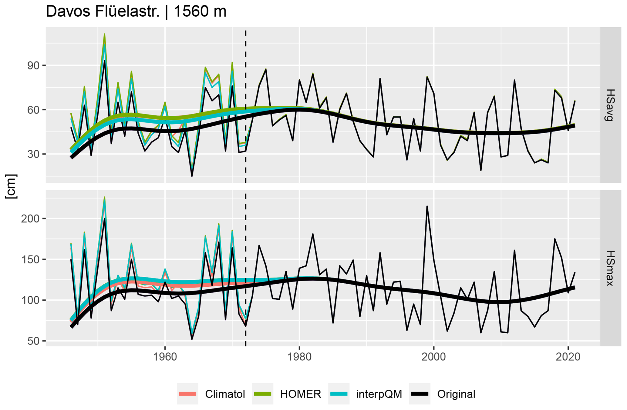
Figure 3Comparison of original and homogenised seasonal mean (HSavg) and maximum (HSmax) snow depths for the SLF station in Davos. The thick lines show a Gaussian-filtered time series with a 30-year window and the vertical dashed line the identified break in 1972.
4.2 Trends of mean and maximum snow depth
The effect of homogenisation on the mean (HSavg) and maximum (HSmax) snow depths is illustrated using the example of Davos in Fig. 3. The adjustments made increased the seasonal mean snow depth before the break in 1972 between 2 and 11 cm with interpQM, between 3 and 17 cm with Climatol and between 3 and 18 cm with HOMER. The impact on the seasonal maximum snow depth ranged from 2 to 19 cm with Climatol, from 7 to 23 cm with interpQM and from 7 to 26 cm with HOMER.
To assess the impact of homogenisation on trends of HSavg and HSmax, decadal trends are calculated for each homogenisation method and the original data, respectively. Figure 4 shows the trends for HSavg in the left panel and for HSmax in the right panel. Trends are expressed in centimetre per decade for the period from 1961 to 2021 for each method and station of the non-homogeneous sub-set, and black dots indicate significant trends. For HSavg, we found an overall similar pattern across the methods. Figure A3 shows the trends as differences between original and homogenised values for Climatol, HOMER and interpQM for both HSavg and HSmax separately. Two of the original series (St. Moritz, Unterwasser-Iltios) show positive trends, whereas HOMER displays positive trends for Simplon and Glarus. No trends are positive with interpQM or Climatol. Except for Glarus (HOMER), none of the positive trends is significant. Homogenisation made the HSavg trends of 17 (HOMER) and 18 (Climatol, interpQM) of the 40 stations either negative or more negative and of 21 (interpQM), 22 (Climatol) or 23 (HOMER) less negative, respectively. Table 3 describes the mean and median trends across all stations as well as the change from positive to negative and significant to non-significant and vice versa for both HSavg and HSmax. The mean trends of HSavg for Climatol and HOMER appear to be weaker than for the original and homogenised interpQM.
Figure 4 further reveals that the homogenised trends for HSavg mimic the pattern of the original trends, which shows almost zero trends for stations below 500 m, strong negative and significant trends for the group between 1000 and 1500 m, followed by mostly non-significant trends for stations between 1500 and 1600 m a.s.l. This suggests that the various intrinsic ways of building reference series and sub-networks of the underlying homogenisation methods do not have a significant impact on decadal trends of HSavg.
The vast majority of the trends for HSmax, 37 of the original series and 39 for all the homogenisation methods, show a negative trend, as shown on the right-hand side of Table 3 for details. The number of significant trends is about 20 % lower than for HSavg, with interpQM showing the largest and HOMER the lowest number of significant trends. The most striking difference between the patterns of HSavg and HSmax in Fig. 4 is the area without significant trends. This is between 1500 and 1600 m a.s.l. for HSavg for all homogenisation methods and below 1000 m a.s.l. for HSmax, with the exception of time series adjusted by interpQM. There seems be no particular altitudinal pattern, except that the trends below 1000 m a.s.l. are weak for all the methods and increase in strength between 1200 and 1400 m a.s.l. This suggests that the trends for HSmax, in contrast to HSavg, appear to be more sensitive to the underlying homogenisation methods.
The performed KS test for revealing noticeable differences between the original and adjusted HSavg time series showed significant differences for four stations for HOMER (Meien, Klosters, Sils-Maria, Stans) and two each for Climatol (Meien, Sils-Maria) and interpQM (Klosters, Stans). The W test showed similar results with six stations for HOMER (Meien, Klosters, St. Moritz, Glarus, Sils-Maria, Stans), five for Climatol (Meien, Klosters, St. Moritz, Glarus, Sils-Maria, Stans) and one for interpQM (Klosters). For a comparison of the results of the adjustment methods, the homogenised time series were compared against each other with the KS and W tests. With the KS test, significant differences were found for all the methods for two stations (Glarus, Stans). The W-test results were also significant between HOMER and Climatol for two stations (Luzern, Stans). For HSmax, the KS test showed significant differences between the original and adjusted time series for three stations for HOMER and interpQM (Klosters, St. Moritz, Elm) and two stations for Climatol (Klosters, St. Moritz). The W test was significant for four stations with HOMER and interpQM (Klosters, St. Moritz, Elm, Sils-Maria) and three with Climatol (Klosters, St. Moritz, Sils-Maria). The adjustment methods were significantly different only with the W test for three stations (La Comballaz, Saanenmöser, Samedan) between HOMER and Climatol.
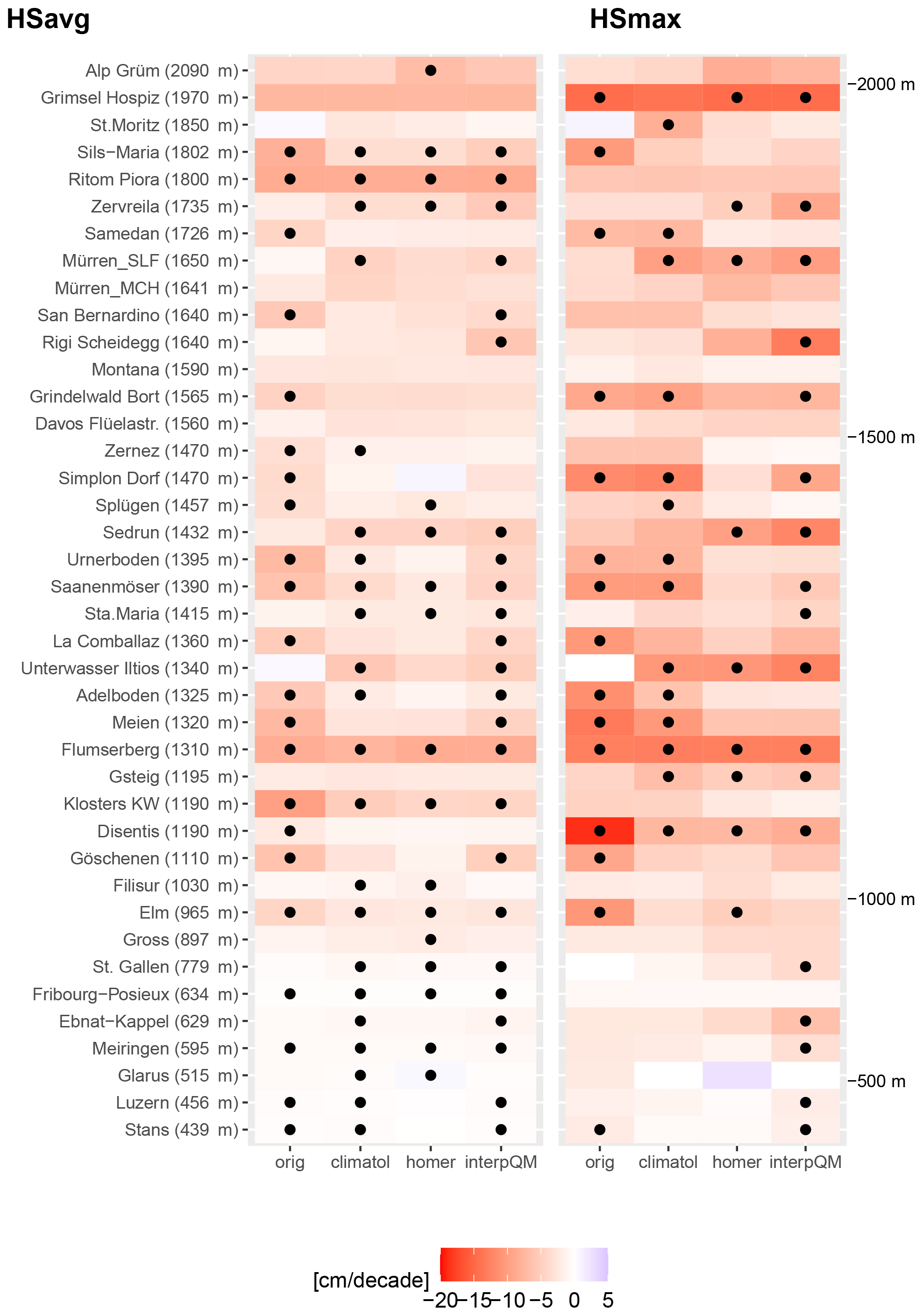
Figure 4Comparison of trends calculated with original and homogenised data (Climatol, HOMER, and interpQM) for the period 1961–2021 for HSavg (left-hand side) and HSmax (right-hand side). Stations are ordered according to elevation. Black dots indicate statistical significance with p values below 0.05.
Table 3Statistics for trends of HSavg and HSmax for the period 1961 to 2021.
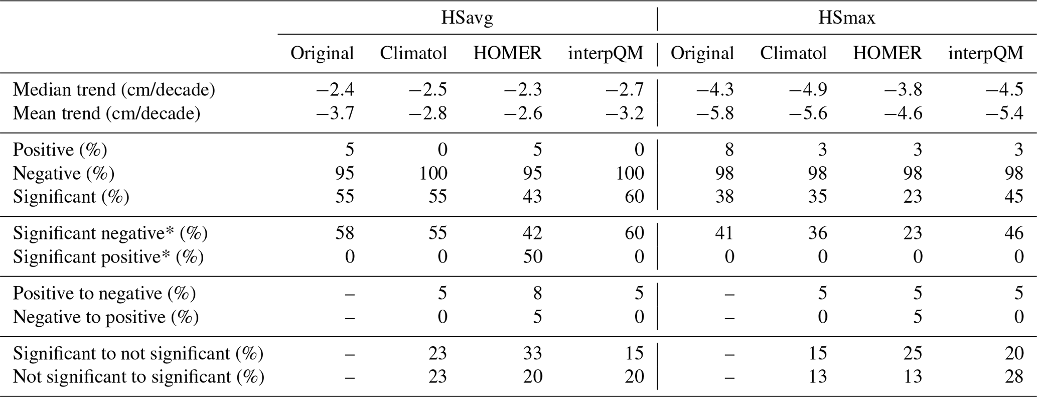
Percentages for significant negative and significant positive, indicated with an asterisk, are calculated based on the total number of negative/positive values, respectively.
4.3 Impact on extreme snow depths
To investigate a possible influence of the homogenisation on the magnitude and frequency of extreme snow depths, the absolute maximum snow depths (maxHSmax) recorded at each station over the entire period, the year with the absolute maximum snow depth and the difference between the original and homogenised maxHSmax are plotted for each station and homogenisation method. Figure 5 shows the results. Here we found that for the majority of series, the differences are 0. The differences are generally left-skewed, except for the largest differences observed with Climatol (Fig. 5d). This again suggests that, in contrast to the trends for HSavg, the differences between the methods are more apparent for HSmax. Furthermore, Fig. 5c clearly highlights the four known snow-rich winters of 1951, 1968, 1975 and 1999.
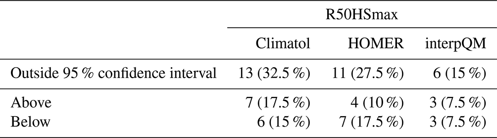
The return levels for 50-year return periods of maximum snow depth (R50HSmax) are calculated from homogenised data and compared with the values obtained from the original data including the 95 % confidence intervals. Figure 6 shows the original values in grey with the associated 95 % confidence intervals and the homogenised values in colour. A pattern was found to occur in all methods for the majority of the stations. For Climatol, seven stations are above the 95 % confidence intervals of the original values for R50HSmax and six below, for HOMER there are four above and seven below, while for interpQM there are three above and three below; see Table 4 for details. This again suggests that the differences between the homogenisation methods are more pronounced for R50HSmax than for trends of HSavg, with interpQM performing slightly better than Climatol or HOMER. An additional analysis (not shown here) of the change in the 95 % confidence intervals shows that the 95 % confidence intervals of the homogenised values are smaller than the original ones. The mean values of R50HSmax across all 40 stations range from 89 cm for the original to 75 cm (HOMER), with Climatol (87 cm) and interpQM (83 cm) in between.

Figure 5Maximum values of HSmax recorded for each station and method over the entire period (1961–2021). Panel (a) shows the year for which the absolute maximum snow depth is recorded. Panel (b) displays the differences between original and homogenised values. Panels (c) and (d) are the corresponding histograms.
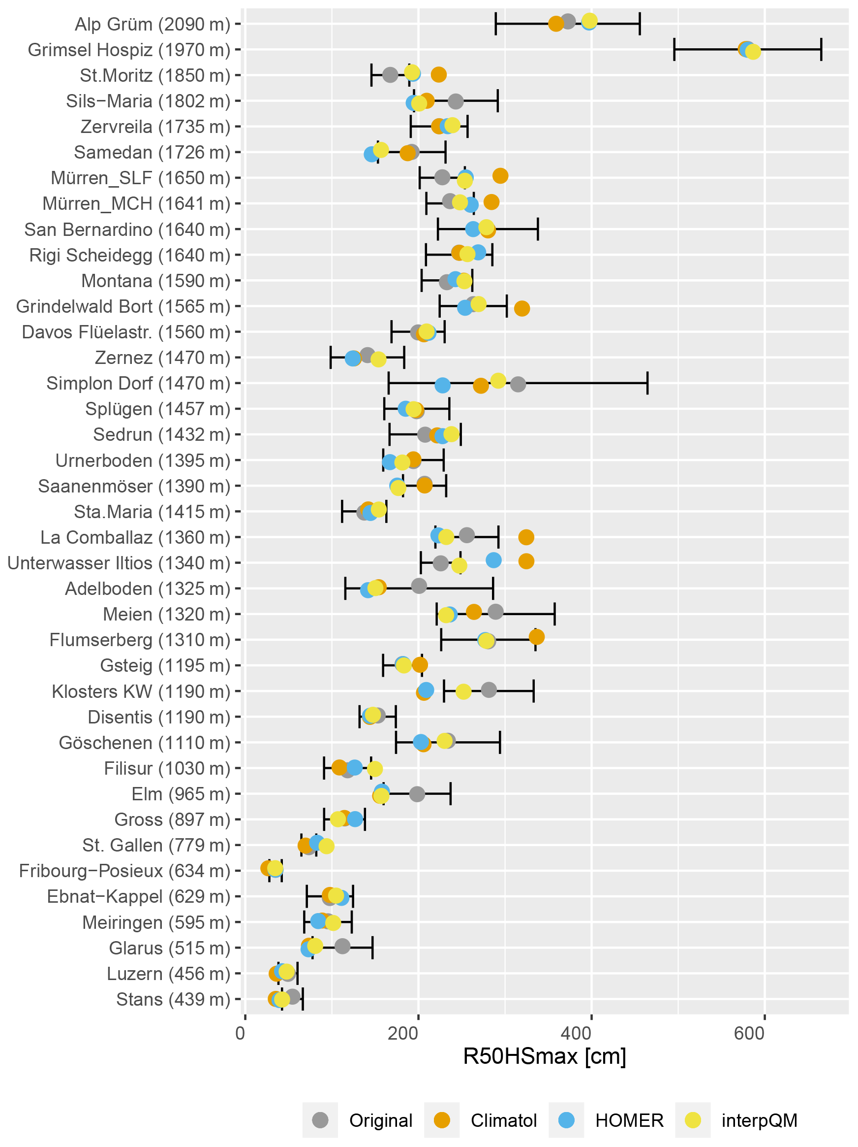
Figure 6HSmax with 50-year return periods and 95 % confidence intervals for both original (grey) and homogenised data using Climatol (orange), HOMER (blue), and interpQM (yellow). The whiskers represent the 95 % confidence interval for the original values. Stations are ordered according to elevation.
Table 4Statistics for R50HSmax: number and percentage of stations that are outside the original's 95 % confidence intervals for each homogenisation method.
The three methods agreed in decreasing the snow depth in the time prior to the breaks for 19 (48 %) of the 40 stations while increasing it for 17 (43 %). For four (9 %) stations, the methods had different signs for the adjustments. The differences between the homogenisation methods were more pronounced for R50HSmax and HSmax than for HSavg.
In contrast to the larger thresholds of the snow day analysis, dHS5 shows almost no differences between the original and homogenised series, confirming the stability of this metric as described by Buchmann et al. (2021b). The elevation-dependent pattern with the strongest adjustment effects for dHS30 and dHS50 between 1000 and 1700 m can be explained by the fact that, firstly, at stations below 1000 m a.s.l. there are few days with a snow depth of 30 cm or more due to the generally warmer temperature and lower snowfall amount and, secondly, that above 1700 m winter temperatures are low enough and therefore less sensitive to warming in winter, so that the trends are smaller. A similar pattern can be seen in the absolute values (Appendix A1). Those high-elevation stations that show large differences in the trends before and after the homogenisation in Fig. 2 (Sils-Maria, Samedan, San Bernardino, Zernez, Simplon Dorf, Splügen) are all located at sites strongly influenced by southerly flows. In particular, the Engadine in the southeast, a high-elevation inner-Alpine valley with a dry and cold climate, is often not associated with large snow depths or many days with dHS30 or dHS50.
All but two of the trends for HSavg (in both the original and homogenised data) are negative, which is consistent with the findings from previous snow studies (Laternser and Schneebeli, 2003; Marty, 2008; Scherrer et al., 2013; Fontrodona Bach et al., 2018; Matiu et al., 2021). Marcolini et al. (2019) report an increase in series showing significant trends for HSavg after homogenisation (40 % to 44 %). The same effect is observed here for interpQM but not for Climatol (no change) and HOMER. Both show a decrease in significant negative trends after homogenisation (Table 3). The same increase in the number of significant negative trends is observed for snow days and HSmax. The adjustments decreased the snow depth prior to a break at 55 % and increased it at 45 % of the stations.
For most stations, the R50HSmax of the homogenised data is still within the 95 % confidence intervals of the original values. However, depending on the homogenisation method, between 3 and 7 of the investigated 40 stations (see Table 4) have an R50HSmax that exceeds the original values beyond the 95 % confidence intervals, with potential implications for engineering applications and building codes. Values that are significantly above the 95 % intervals are predominantly from Climatol. The reference networks in Climatol are created using the Euclidean distances between candidate and reference series, with an optional scaling factor for the vertical component. We set this threshold to wz=100 to avoid the selection of stations that are close together horizontally but far apart vertically, e.g. the stations Davos (1570 m a.s.l.) and Weissfluhjoch (2535 m a.s.l.), which are only 4 km apart horizontally. However, it may also be that this threshold is simply not low enough to prevent further station combinations with a similarly large gradient. Unfortunately, the user cannot see in Climatol which series were used as a reference for a particular station. The reduction of the 95 % confidence intervals for all methods after homogenisation indicates a decrease in variation and an increase in confidence in the results for very large snow depths, as shown with the absolute maximum snow depth.
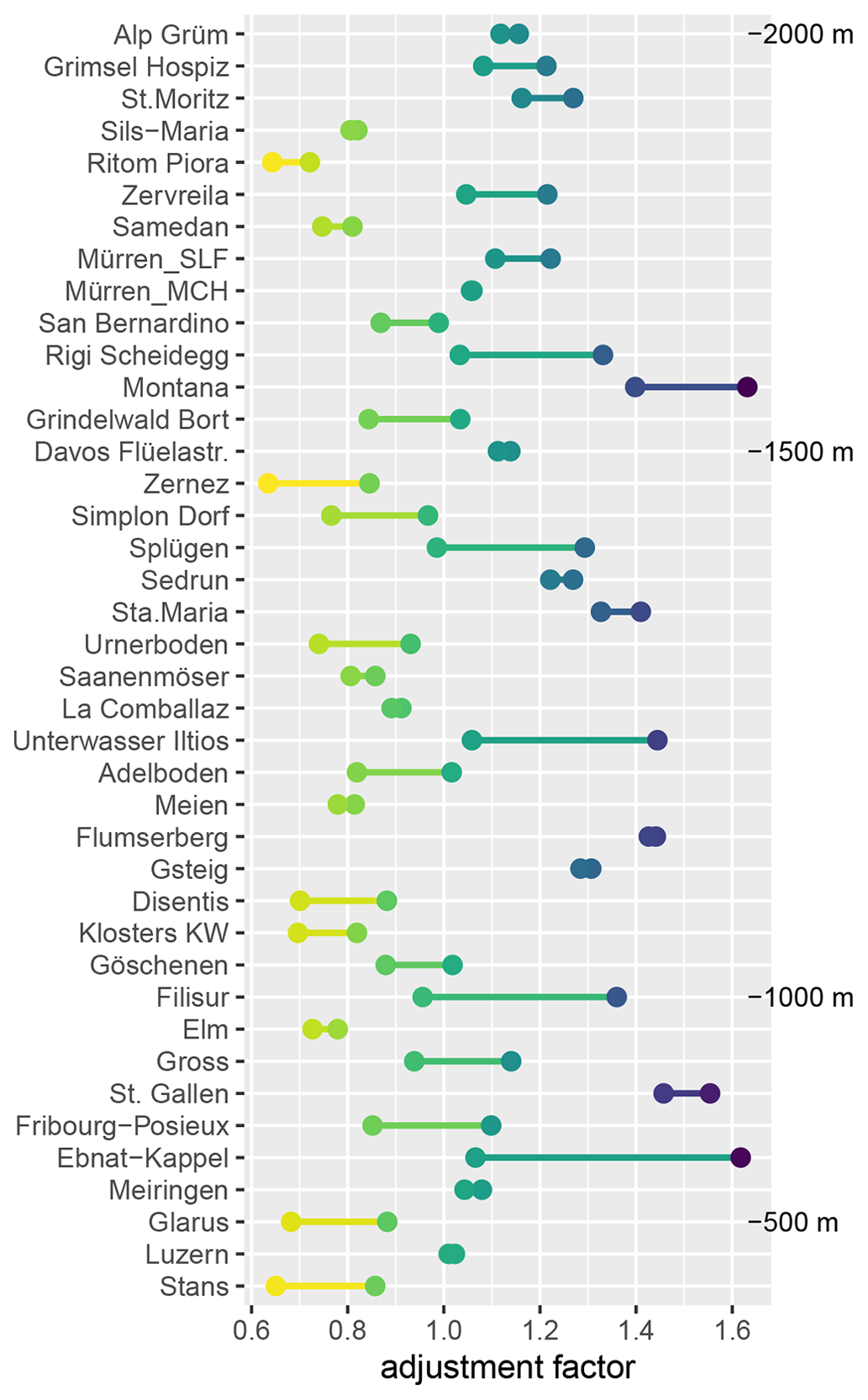
The observed differences between the three methods compared can be explained by the respective methods used to construct the reference series sub-networks and the adjustments. HOMER adjusts the entire period before an identified break point using a single factor, while Climatol uses multiple factors dependent on the reference series constructed using homogenised sub-periods. interpQM, on the other hand, uses multiple adjustment factors based on quantile matching for the entire inhomogeneous period, similarly to HOMER. The range of the applied adjustments for interpQM is shown in Appendix A4.
The selection of suitable reference series is the crucial part of the homogenisation procedure, both for the detection of breaks and for the adjustment step. HOMER can be run in either correlation or distance mode: i.e. the sub-networks are compiled based on thresholds for either correlation or horizontal distances. In Climatol, the sub-networks are formed based on the Euclidean distance between series with a scaling parameter for the vertical component. In interpQM, the user can choose correlation and horizontal as well as vertical distance thresholds. For a height-dependent variable such as snow depth, the ability to select the sub-networks by setting thresholds for vertical and horizontal distances separately proves invaluable. It is possible, albeit cumbersome, to define the sub-networks manually and use them as input for HOMER. The ability in HOMER to visually inspect the set of reference series used for each candidate station can provide a useful indication of how accurately the reference series reflect local climatic or topographic characteristics: for example, does the majority of the reference series come from a completely different micro-climate? This is particularly important for a study area with complex Alpine topography, where neighbouring valleys may have completely different climates: northern/southern, inner-Alpine, or pre-Alpine. Furthermore, these lists of reference series can also be used to identify stations with suspicious reference series that are probably not suitable for homogenisation.
The analysis of the sub-networks for HOMER and interpQM shows that, due to the distance restriction in interpQM, reference series are drawn from a more similar region, whereas in HOMER distant stations with high correlations are frequently included. To avoid selecting close-by but unsuitable reference series due to local climatic variations, the correlation criterion in interpQM works well.
Both Marcolini et al. (2019) and Buchmann et al. (2022a) found that relocations were responsible for by far the most detected break points in snow depth time series. The metadata of many stations are sparse and therefore often do not provide enough information to give a sufficient answer to the question of why a relocation caused a break. A change in elevation within ±150 m is not necessarily a cause of a break, but moving a station either below or above the typical height of a site's inversion is highly likely. Significant changes in the station environment are also very likely to cause a break, e.g. moving a station to an area with fewer buildings or fewer and smaller trees and vice versa.
This study is the first in-depth comparison of different homogenisation methods applied to a large network of snow depth series between 500 and 2500 m. The focus is on their influence on the decadal trends of the number of snow days, i.e. days with a snow depth above a certain threshold (5, 30 and 50 cm), the seasonal mean and maximum snow depths (HSavg, HSmax) and extreme snow depths. The results underpin the relevance of homogenising long-term snow depth series for trend and extreme value analysis. Due to the impact of homogenisation on derived trends, this is especially true for conclusions drawn from individual series. In our analyses, for the long-term trends of HSavg and dHS5, the overall picture does not change through homogenisation of original data by median-/mean-based adjustment methods. However, the picture becomes different when a quantile-based homogenisation approach (interpQM) is applied, which in the case of Swiss snow depth series shows the strongest effect, with only negative trends for HSavg and a slight increase in the number of significant trends. The differences between the methods increase when looking at seasonal maximum values: the trends for HSmax, where trends of low-elevation stations were significant only with interpQM, absolute maximum snow depths and extreme values. The homogenisation performed with interpQM increases the confidence in the derived extreme values based on the 95 % confidence interval, which is particularly relevant for engineering applications. As far as snow days are concerned, the quantile-based adjustments had the strongest impact on the larger snow depth thresholds.
Our results support a homogenisation approach that separates the break point detection from the adjustment procedure, e.g. to use the robust combined detection approach described in Buchmann et al. (2022b) in combination with the adjustment procedure from Resch et al. (2022). However, the ability to manually adjust the automatic selection of the reference (sub-network) stations used for homogenisation is crucial for optimising the results. A combination of criteria such as correlation, horizontal and vertical distances as well as manual interventions seems to be more advantageous (given the complex topography in mountain regions like the Alps) for snow depth than the use of a single selection criterion.
So far, the homogenised snow depth time series have shown no evidence of a bias in the methods towards increasing or decreasing snow depths due to the adjustments made, neither in Austria nor in Switzerland. In this study, depending on the homogenisation method, the mean snow depth before a break was increased at about 52 %–57 % of the stations and decreased at between 42 % and 45 % of them; 95 % of the 40 inhomogeneous stations show a negative trend for seasonal mean snow depth in the original data, which is significant for 58 %. These figures are lower for the 144 homogeneous stations in the data set, where 78 % show a negative trend that is significant for 50 %.
As pointed out, break detection for snow depth is preferably done using the described two-out-of-three method. From our experience, there is no incentive or advantage to using automatic homogenisation methods such as HOMER and Climatol. On the contrary, automatic methods open the door to unintended automatic outlier corrections or adjustments based on the selection of reference series that are sufficiently correlated but that cannot be assigned in a climatologically meaningful way. To achieve reasonable results, these methods require a certain degree of user intervention, e.g. the use of a pre-defined selection of reference stations, thresholds for correlation, and horizontal and vertical distances. Therefore, it seems promising to separate the detection and adjustment of breaks using the described two-out-of-three method for detection and interpQM for the adjustment, as it provides reliable results, especially for larger snow depths, and yields daily data.

Figure A1Absolute trends for days with snow depths of at least 5, 30 and 50 cm per season. Significant trends are marked by a black border.
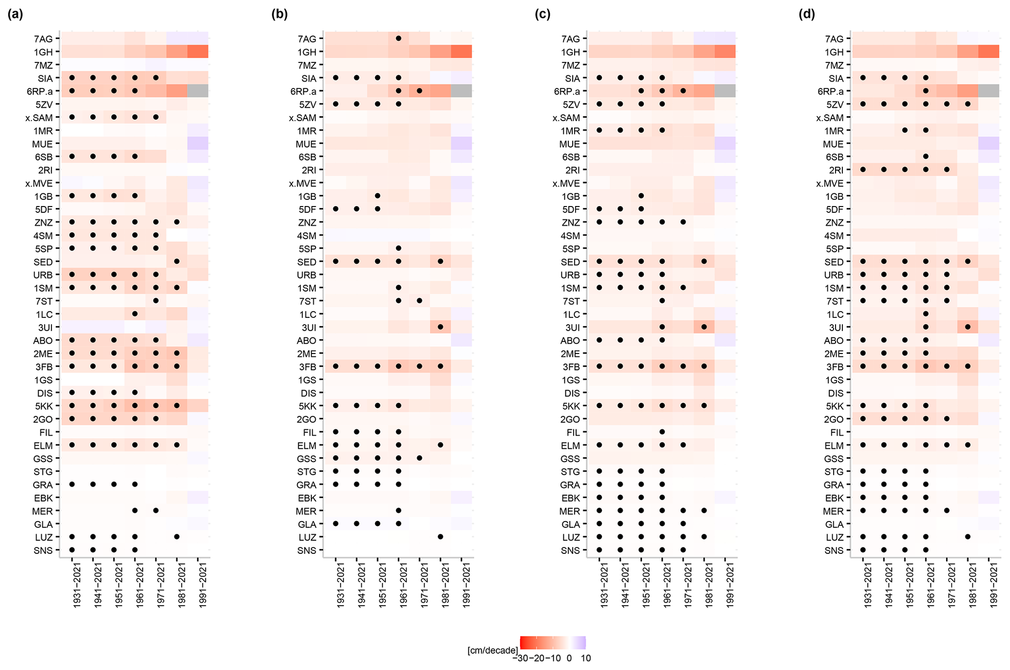
Figure A2Trends for HSavg: shown are all methods and all decades. Original (a), HOMER (b), Climatol (c), and interpQM (d).
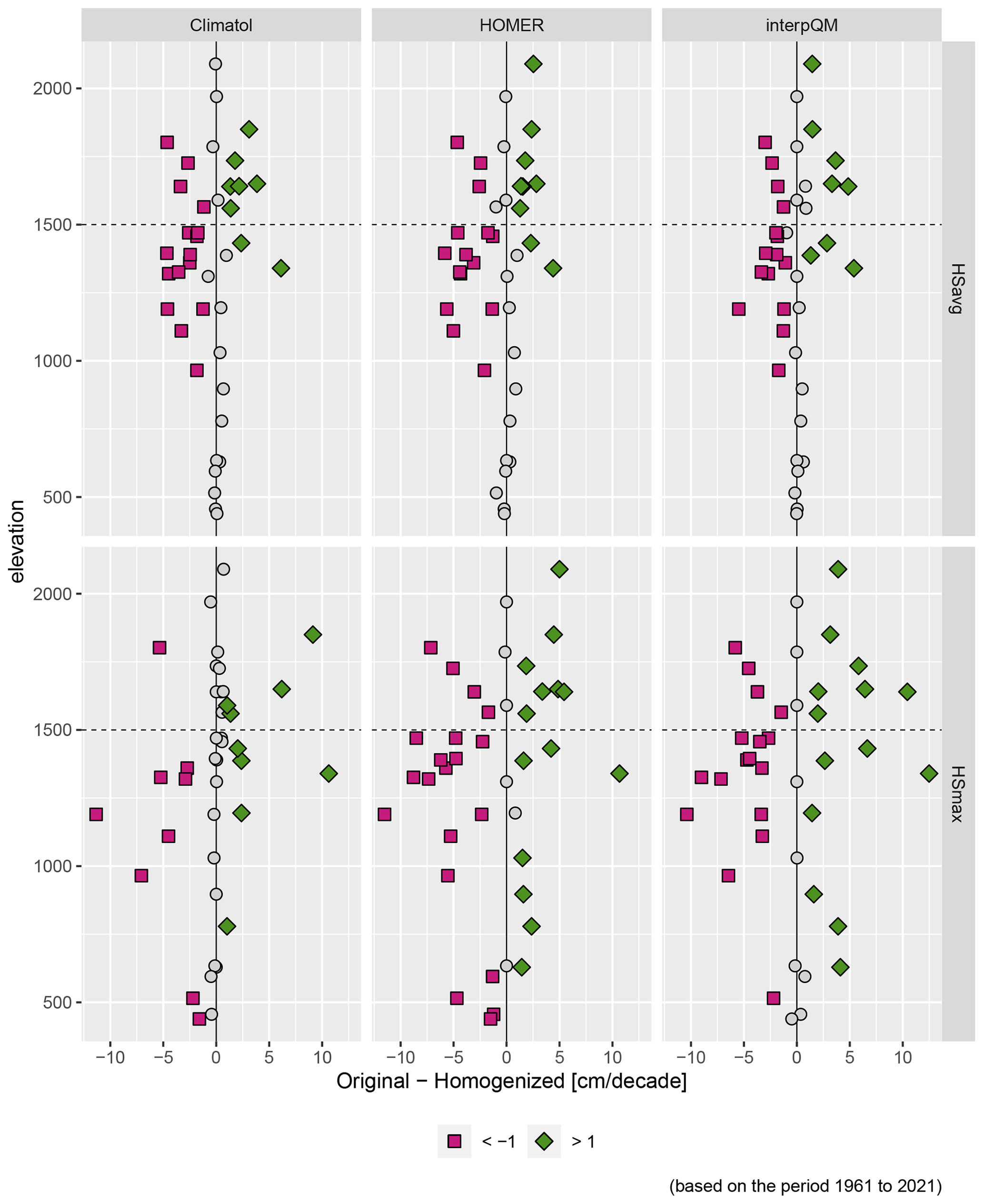
Figure A3Comparison of differences of trends calculated with Climatol, HOMER, and interpQM for the period 1961–2021 for HSavg and HSmax. Differences are calculated as original − homogenised. Purple squares indicate stations with a result of , green diamonds >1 d/decade.
Input data for the various homogenisation methods are available on EnviDat at https://doi.org/10.16904/envidat.336 (Buchmann and Resch, 2022).
The study was devised by MBu and CM with input from GR, WS and MBe. Snow day analysis was performed by GR, HSavg and HSmax analysis by MBu. The figures were produced by GR and MBu. GR and MBu discussed the results with input from CM, SB and WS. MBu and GR wrote the initial draft. The article was finalised by GR with contributions from all the co-authors.
The contact author has declared that none of the authors has any competing interests.
Publisher's note: Copernicus Publications remains neutral with regard to jurisdictional claims in published maps and institutional affiliations.
The authors want to thank the two anonymous reviewers for investing their time in improving and polishing our manuscript with ideas and constructive comments. We would also like to thank MeteoSchweiz, SLF, ZAMG and the Austrian Water Budget Department for access to their data sets. For data juggling, homogenisation and evaluation, R 4.2 (R Core Team, 2022) with the tidyverse package (Wickham et al., 2019) as well as R 2.15 were used. We would also like to thank all snow observers. Without their continuous effort, this study would not have been possible. This research was developed with the financial support of the FWF (Fonds zur Förderung der wissenschaftlichen Forschung, project Hom4Snow, grant no. I 3692) and the Schweizerischer Nationalfonds zur Förderung der Wissenschaftlichen Forschung (grant/award no. SNF: 200021L 175920).
This research has been supported by the FWF (Fonds zur Förderung der wissenschaftlichen Forschung, project Hom4Snow, grant no. I 3692) and the Schweizerischer Nationalfonds zur Förderung der Wissenschaftlichen Forschung (grant no. SNF:200021L 175920).
This paper was edited by Masashi Niwano and reviewed by two anonymous referees.
Abegg, B., Morin, S., Demiroglu, O. C., François, H., Rothleitner, M., and Strasser, U.: Overloaded! Critical revision and a new conceptual approach for snow indicators in ski tourism, Int. J. Biometeorol., 65, 701, https://doi.org/10.1007/s00484-020-01867-3, 2020. a, b, c
Alexandersson, H.: A homogeneity test applied to precipitation data, J. Climatol., 6, 661–675, https://doi.org/10.1002/joc.3370060607, 1986. a, b
Alexandersson, H. and Moberg, A.: HOMOGENIZATION OF SWEDISH TEMPERATURE DATA. PART I: HOMOGENEITY TEST FOR LINEAR TRENDS, Int. J. Climatol., 17, 25–34, https://doi.org/10.1002/(SICI)1097-0088(199701)17:1<25::AID-JOC103>3.0.CO;2-J, 1997. a, b, c
Al-Rubaye, S., Maguire, M., and Bean, B.: Design Ground Snow Loads: Historical Perspective and State of the Art, J. Struct. Eng., 148, 03122001, https://doi.org/10.1061/(ASCE)ST.1943-541X.0003339, 2022. a
Armstrong, R. and Brun, E.: Snow and Climate: Physical Processes, Surface Energy Exchange and Modeling, Cambridge University Press, https://doi.org/10.3189/002214309788608741, 2008. a
Auer, I., Böhm, R., Jurkovic, A., Lipa, W., Orlik, A., Potzmann, R., Schöner, W., Ungersböck, M., Matulla, C., Briffa, K., Jones, P., Efthymiadis, D., Brunetti, M., Nanni, T., Maugeri, M., Mercalli, L., Mestre, O., Moisselin, J.-M., Begert, M., Müller-Westermeier, G., Kveton, V., Bochnicek, O., Stastny, P., Lapin, M., Szalai, S., Szentimrey, T., Cegnar, T., Dolinar, M., Gajic-Capka, M., Zaninovic, K., Majstorovic, Z., and Nieplova, E.: HISTALP – historical instrumental climatological surface time series of the Greater Alpine Region, Int. J. Climatol., 27, 17–46, https://doi.org/10.1002/joc.1377, 2007. a, b
Begert, M., Schlegel, T., and Kirchhofer, W.: Homogeneous temperature and precipitation series of Switzerland from 1864 to 2000, Int. J. Climatol., 25, 65–80, https://doi.org/10.1002/joc.1118, 2005. a
Bocchiola, D., Bianchi Janetti, E., Gorni, E., Marty, C., and Sovilla, B.: Regional evaluation of three day snow depth for avalanche hazard mapping in Switzerland, Nat. Hazards Earth Syst. Sci., 8, 685–705, https://doi.org/10.5194/nhess-8-685-2008, 2008. a
Brown, R. D., Brasnett, B., and Robinson, D.: Gridded North American monthly snow depth and snow water equivalent for GCM evaluation, Atmosphere-Ocean, 41, 1–14, https://doi.org/10.3137/ao.410101, 2003. a
Buchmann, M. and Resch, G.: Input data for impact assessment of homogenised snow series, EnviDat [data set], https://doi.org/10.16904/envidat.336, 2022. a
Buchmann, M., Begert, M., Brönnimann, S., and Marty, C.: Local-scale variability of seasonal mean and extreme values of in situ snow depth and snowfall measurements, The Cryosphere, 15, 4625–4636, https://doi.org/10.5194/tc-15-4625-2021, 2021a. a, b
Buchmann, M., Begert, M., Brönnimann, S., and Marty, C.: Evaluating the robustness of snow climate indicators using a unique set of parallel snow measurement series, Int. J. Climatol., 41, E2553–E2563, https://doi.org/10.1002/joc.6863, 2021b. a
Buchmann, M., Aschauer, J., Begert, M., and Marty, C.: Input data for break point detection of Swiss snow depth series, EnviDat [data set], https://doi.org/10.16904/envidat.297, 2022a. a
Buchmann, M., Coll, J., Aschauer, J., Begert, M., Brönnimann, S., Chimani, B., Resch, G., Schöner, W., and Marty, C.: Homogeneity assessment of Swiss snow depth series: comparison of break detection capabilities of (semi-)automatic homogenization methods, The Cryosphere, 16, 2147–2161, https://doi.org/10.5194/tc-16-2147-2022, 2022b. a, b, c, d, e, f
Caussinus, H. and Mestre, O.: Detection and correction of artificial shifts in climate series, J. Roy. Stat. Soc. C, 53, 405–425, https://doi.org/10.1111/j.1467-9876.2004.05155.x, 2004. a, b, c
Cornes, R. C., van der Schrier, G., van den Besselaar, E. J., and Jones, P. D.: An Ensemble Version of the E-OBS Temperature and Precipitation Data Sets, J. Geophys. Res.-Atmos., 123, 9391–9409, https://doi.org/10.1029/2017JD028200, 2018. a
Croce, P., Formichi, P., and Landi, F.: Extreme Ground Snow Loads in Europe from 1951 to 2100, Climate, 9, 133, https://doi.org/10.3390/cli9090133, 2021. a
Domonkos, P.: Adapted Caussinus-Mestre Algorithm for Networks of Temperature series (ACMANT), Int. J. Geosci., 02, 293–309, https://doi.org/10.4236/ijg.2011.23032, 2011. a, b, c
Easterling, D. R. and Peterson, T. C.: A new method for detecting undocumented discontinuities in climatological time series, Int. J. Climatol., 15, 369–377, https://doi.org/10.1002/joc.3370150403, 1995. a
Essery, R., Morin, S., Lejeune, Y., and Ménard, C. B.: A comparison of 1701 snow models using observations from an alpine site, Adv. Water Resour., 55, 131–148, https://doi.org/10.1016/j.advwatres.2012.07.013, 2013. a
Fontrodona Bach, A., van der Schrier, G., Melsen, L. A., Klein Tank, A. M. G., and Teuling, A. J.: Widespread and Accelerated Decrease of Observed Mean and Extreme Snow Depth Over Europe, Geophys. Res. Lett., 45, 12312–12319, https://doi.org/10.1029/2018GL079799, 2018. a
Gilleland, E. and Katz, R. W.: extRemes 2.0: An Extreme Value Analysis Package in R, J. Stat. Softw., 72, 1–39, https://doi.org/10.18637/jss.v072.i08, 2016. a
Gubler, S., Hunziker, S., Begert, M., Croci-Maspoli, M., Konzelmann, T., Brönnimann, S., Schwierz, C., Oria, C., and Rosas, G.: The influence of station density on climate data homogenization, Int. J. Climatol., 37, 4670–4683, https://doi.org/10.1002/joc.5114, 2017. a
Guijarro, J. A.: Homogenization of climatic series with Climatol, Tech. rep., AEMET, https://doi.org/10.13140/RG.2.2.27020.41604, 2018. a, b, c, d
Hersbach, H., Bell, B., Berrisford, P., Hirahara, S., Horányi, A., Muñoz-Sabater, J., Nicolas, J., Peubey, C., Radu, R., Schepers, D., Simmons, A., Soci, C., Abdalla, S., Abellan, X., Balsamo, G., Bechtold, P., Biavati, G., Bidlot, J., Bonavita, M., De Chiara, G., Dahlgren, P., Dee, D., Diamantakis, M., Dragani, R., Flemming, J., Forbes, R., Fuentes, M., Geer, A., Haimberger, L., Healy, S., Hogan, R. J., Hólm, E., Janisková, M., Keeley, S., Laloyaux, P., Lopez, P., Lupu, C., Radnoti, G., de Rosnay, P., Rozum, I., Vamborg, F., Villaume, S., and Thépaut, J. N.: The ERA5 global reanalysis, Q. J. Roy. Meteor. Soc., 146, 1999–2049, https://doi.org/10.1002/qj.3803, 2020. a
Hiebl, J. and Frei, C.: Daily precipitation grids for Austria since 1961 – development and evaluation of a spatial dataset for hydroclimatic monitoring and modelling, Theor. Appl. Climatol., 132, 327–345, https://doi.org/10.1007/s00704-017-2093-x, 2018. a
Johnston, A. N., Bruggeman, J. E., Beers, A. T., Beever, E. A., Christophersen, R. G., and Ransom, J. I.: Ecological consequences of anomalies in atmospheric moisture and snowpack, Ecology, 100, 1–12, https://doi.org/10.1002/ecy.2638, 2019. a
Jonas, T., Rixen, C., Sturm, M., and Stoeckli, V.: How alpine plant growth is linked to snow cover and climate variability, J. Geophys. Res.-Biogeo., 113, G03013, https://doi.org/10.1029/2007JG000680, 2008. a
Kendall, M.: Rank Correlation Methods, Charles Griffin, 4th edn., Second Impression, Charles Griffin & Company, Ltd., London, 202 pp., 1975. a
Kuglitsch, F. G., Toreti, A., Xoplaki, E., Della-Marta, P. M., Luterbacher, J., and Wanner, H.: Homogenization of daily maximum temperature series in the Mediterranean, J. Geophys. Res.-Atmos., 114, D15108, https://doi.org/10.1029/2008JD011606, 2009. a
Laternser, M. and Schneebeli, M.: Long-term snow climate trends of the Swiss Alps (1931–99), Int. J. Climatol., 23, 733–750, https://doi.org/10.1002/joc.912, 2003. a
Li, Q., Yang, T., and Li, L.: Evaluation of snow depth and snow cover represented by multiple datasets over the Tianshan Mountains: Remote sensing, reanalysis, and simulation, Int. J. Climatol., 42, 4223–4239, https://doi.org/10.1002/joc.7459, 2022. a
Mann, H.: Nonparametric tests against trend, Econometrica, 13, 245–259, 1945. a
Maraun, D., Shepherd, T. G., Widmann, M., Zappa, G., Walton, D., Gutiérrez, J. M., Hagemann, S., Richter, I., Soares, P. M., Hall, A., and Mearns, L. O.: Towards process-informed bias correction of climate change simulations, Nat. Clim. Change, 7, 764–773, https://doi.org/10.1038/nclimate3418, 2017. a
Marcolini, G., Bellin, A., and Chiogna, G.: Performance of the Standard Normal Homogeneity Test for the homogenization of mean seasonal snow depth time series, Int. J. Climatol, 37, 1267–1277, https://doi.org/10.1002/joc.4977, 2017. a
Marcolini, G., Koch, R., Chimani, B., Schöner, W., Bellin, A., Disse, M., and Chiogna, G.: Evaluation of homogenization methods for seasonal snow depth data in the Austrian Alps, 1930–2010, Int. J. Climatol., 39, 4514–4530, https://doi.org/10.1002/joc.6095, 2019. a, b, c
Marke, T., Strasser, U., Hanzer, F., Stötter, J., Wilcke, R. A. I., and Gobiet, A.: Scenarios of Future Snow Conditions in Styria (Austrian Alps), J. Hydrometeorol., 16, 261–277, https://doi.org/10.1175/JHM-D-14-0035.1, 2015. a
Marty, C.: Regime shift of snow days in Switzerland, Geophys. Res. Lett., 35, L12501, https://doi.org/10.1029/2008GL033998, 2008. a, b
Marty, C. and Blanchet, J.: Long-term changes in annual maximum snow depth and snowfall in Switzerland based on extreme value statistics, Clim. Change, 111, 705–721, https://doi.org/10.1007/s10584-011-0159-9, 2012. a, b, c
Marty, C., Schlögl, S., Bavay, M., and Lehning, M.: How much can we save? Impact of different emission scenarios on future snow cover in the Alps, The Cryosphere, 11, 517–529, https://doi.org/10.5194/tc-11-517-2017, 2017. a
Matiu, M., Crespi, A., Bertoldi, G., Carmagnola, C. M., Marty, C., Morin, S., Schöner, W., Cat Berro, D., Chiogna, G., De Gregorio, L., Kotlarski, S., Majone, B., Resch, G., Terzago, S., Valt, M., Beozzo, W., Cianfarra, P., Gouttevin, I., Marcolini, G., Notarnicola, C., Petitta, M., Scherrer, S. C., Strasser, U., Winkler, M., Zebisch, M., Cicogna, A., Cremonini, R., Debernardi, A., Faletto, M., Gaddo, M., Giovannini, L., Mercalli, L., Soubeyroux, J.-M., Sušnik, A., Trenti, A., Urbani, S., and Weilguni, V.: Observed snow depth trends in the European Alps: 1971 to 2019, The Cryosphere, 15, 1343–1382, https://doi.org/10.5194/tc-15-1343-2021, 2021. a, b, c
Mestre, O., Domonkos, P., Picard, F., Auer, I., Robin, S., Lebarbier, E., Boehm, R., Aguilar, E., Guijarro, J., Vertachnik, G., Klancar, M., Dubuisson, B., and Stepanek, P.: HOMER: a homogenization software – methods and applications, IDOJARAS, 117, 47–67, 2013. a, b, c
Morin, S., Horton, S., Techel, F., Bavay, M., Coléou, C., Fierz, C., Gobiet, A., Hagenmuller, P., Lafaysse, M., Ližar, M., Mitterer, C., Monti, F., Müller, K., Olefs, M., Snook, J. S., van Herwijnen, A., and Vionnet, V.: Application of physical snowpack models in support of operational avalanche hazard forecasting: A status report on current implementations and prospects for the future, Cold Reg. Sci. Technol., 170, 102910, https://doi.org/10.1016/j.coldregions.2019.102910, 2020. a
Nemec, J., Gruber, C., Chimani, B., and Auer, I.: Trends in extreme temperature indices in Austria based on a new homogenised dataset, Int. J. Climatol., 33, 1538–1550, https://doi.org/10.1002/joc.3532, 2013. a
Nitu, R., Roulet, Y., Wolff, M., Earle, M., Reverdin, A., Smith, C., Kochendorfer, J., Morin, S., Rasmussen, R., Wong, K., Alastrué, J., Arnold, L., Baker, B., Buisan, S., Collado, J. L., Colli, M., Collins, B., Gaydos, A., Hannula, H.-R., Hoover, J., Joe, P., Kontu, A., Laine, T., Lanza, L., Lanzinger, E., Lee, G. W., Lejeune, Y., Leppänen, L., Mekis, E., Panel, J., Poikonen, A., Ryu, S., Sabatini, F., Theriault, J., Yang, D., Genthon, C., van den Heuvel, F., Hirasawa, N., Konishi, H., Nishimura, K., and Senese, A.: WMO Solid Precipitation Intercomparison Experiment (SPICE) (2012–2015), techreport 131, WMO, https://library.wmo.int/index.php?lvl=notice_display&id=20742 (last access: 6 February 2023), 2018. a
Olefs, M., Schöner, W., Suklitsch, M., Wittmann, C., Niedermoser, B., Neururer, A., and Wurzer, A.: SNOWGRID – A New Operational Snow Cover Model in Austria, International Snow Science Workshop Grenoble – Chamonix Mont-Blanc, 7–11 October 2013, 38–45, https://www.researchgate.net/publication/281377426 (last access: 6 February 2023), 2013. a
Picard, F., Lebarbier, E., Hoebeke, M., Rigaill, G., Thiam, B., and Robin, S.: Joint segmentation, calling, and normalization of multiple CGH profiles, Biostatistics, 12, 413–428, https://doi.org/10.1093/biostatistics/kxq076, 2011. a
Pulliainen, J., Luojus, K., Derksen, C., Mudryk, L., Lemmetyinen, J., Salminen, M., Ikonen, J., Takala, M., Cohen, J., Smolander, T., and Norberg, J.: Patterns and trends of Northern Hemisphere snow mass from 1980 to 2018, Nature, 581, 294–298, https://doi.org/10.1038/s41586-020-2258-0, 2020. a
R Core Team: R: A Language and Environment for Statistical Computing, R Foundation for Statistical Computing, Vienna, Austria, https://www.R-project.org/ (last access: 6 February 2023), 2022. a
Resch, G., Koch, R., Marty, C., Chimani, B., Begert, M., Buchmann, M., Aschauer, J., and Schöner, W.: A quantile-based approach to improve homogenization of snow depth time series, Int. J. Climatol., 43, 173, https://doi.org/10.1002/joc.7742, 2022. a, b, c, d, e
Schellander, H., Winkler, M., and Hell, T.: Towards a reproducible snow load map – an example for Austria, Adv. Sci. Res., 18, 135–144, https://doi.org/10.5194/asr-18-135-2021, 2021. a, b
Scherrer, S. C., Appenzeller, C., and Laternser, M.: Trends in Swiss Alpine snow days: The role of local- and large-scale climate variability, Geophys. Res. Lett., 31, L13215, https://doi.org/10.1029/2004GL020255, 2004. a
Scherrer, S. C., Wüthrich, C., Croci-Maspoli, M., Weingartner, R., and Appenzeller, C.: Snow variability in the Swiss Alps 1864–2009, Int. J. Climatol., 33, 3162–3173, https://doi.org/10.1002/joc.3653, 2013. a, b
Schmucki, E., Marty, C., Fierz, C., Weingartner, R., and Lehning, M.: Impact of climate change in Switzerland on socioeconomic snow indices, Theor. Appl. Climatol., 127, 875–889, https://doi.org/10.1007/s00704-015-1676-7, 2017. a
Schöner, W., Koch, R., Matulla, C., Marty, C., and Tilg, A.-M.: Spatiotemporal patterns of snow depth within the Swiss-Austrian Alps for the past half century (1961 to 2012) and linkages to climate change, Int. J. Climatol., 39, 1589–1603, https://doi.org/10.1002/joc.5902, 2019. a
Sen, P.: Estimates of the regression coefficient based on Kendall's tau, J. Am. Stat. A., 63, 1379–1389, 1968. a
Stone, R. S., Dutton, E. G., Harris, J. M., and Longenecker, D.: Earlier spring snowmelt in northern Alaska as an indicator of climate change, J. Geophys. Res.-Atmos., 107, ACL 10-1–ACL 10-13, https://doi.org/10.1029/2000JD000286, 2002. a
Theil, H.: A rank‐invariant method of linear and polynomial regression analysis, Proc. Konink. Nederl. Akad. Wetensch. Ser. A Math. Sci., 53, 1412, 1950. a
Venema, V., Trewin, B., and Wang, X.: Guidelines on Homogenization 2020 edition, Tech. rep., World Meteorological Organization Issue WMO-No. 1245, https://library.wmo.int/?lvl=notice_display&id=21756 (last access: 6 February 2023), 2020. a, b
Vincent, L. A., Zhang, X., Bonsal, B. R., and Hogg, W. D.: Homogenization of Daily Temperatures over Canada, J. Climate, 15, 1322–1334, https://doi.org/10.1175/1520-0442(2002)015<1322:HODTOC>2.0.CO;2, 2002. a
Wickham, H., Averick, M., Bryan, J., Chang, W., Mcgowan, L. D. A., François, R., Grolemund, G., Hayes, A., Henry, L., Hester, J., Kuhn, M., Lin, T., Miller, E., Bache, S. M., Müller, K., Ooms, J., Robinson, D., Seidel, D. P., Spinu, V., Takahashi, K., Vaughan, D., Wilke, C., and Woo, K.: Welcome to the Tidyverse, J. Open Source Softw., 4, 1–6, https://doi.org/10.21105/joss.01686, 2019. a
Yue, S., Pilon, P., Phinney, B., and Cavadias, G.: The influence of autocorrelation on the ability to detect trend in hydrological series, Hydrol. Process., 16, 1807–1829, https://doi.org/10.1002/hyp.1095, 2002. a