the Creative Commons Attribution 4.0 License.
the Creative Commons Attribution 4.0 License.
 | 07 Dec 2023
Spatiotemporal snow water storage uncertainty in the midlatitude American Cordillera
Yiwen Fang
Yufei Liu
Dongyue Li
Haorui Sun
Steven A. Margulis
This work quantifies the uncertainty of accumulation-season peak snow water storage in the portions of the midlatitude American Cordillera where snow is a dominant driver of hydrology. This is accomplished through intercomparison of commonly used global and regional products over the Western United States (WUS) and Andes domains, which have similar hydrometeorology but are disparate with respect to the amount of available in situ information. The recently developed WUS Snow Reanalysis (WUS-SR) and Andes Snow Reanalysis (Andes-SR) datasets, which have been extensively verified against in situ measurements, are used as baseline reference datasets in the intercomparison. Relative to WUS-SR climatological peak snow water equivalent (SWE) storage (269 km3), high- and moderate-resolution products (i.e., those with resolutions less than ∼10 km) are in much better agreement (284±14 km3; overestimated by 6 %) compared to low-resolution products (127±54 km3; underestimated by 53 %). In comparison to the Andes-SR peak snow storage (29 km3), all other products show large uncertainty and bias (19±16 km3; underestimated by 34 %). Examination of spatial patterns related to orographic effects showed that only the high- to moderate-resolution Snow Data Assimilation System (SNODAS) and University of Arizona (UA) products show comparable estimates of windward–leeward SWE patterns over a subdomain (Sierra Nevada) of the WUS. Coarser products distribute too much snow on the leeward side in both the Sierra Nevada and Andes, missing orographic and rain shadow patterns that have important hydrological implications. The uncertainty of peak seasonal snow storage is primarily explained by precipitation uncertainty in both the WUS (R2=0.55) and Andes (R2=0.84). Despite using similar forcing inputs, snow storage diverges significantly within the ECMWF Reanalysis v5 (ERA5) (i.e., ERA5 vs. ERA5-Land) products and the Global Land Data Assimilation System (GLDAS) (modeled with Noah, Variable Infiltration Capacity (VIC), and Catchment model) products due to resolution-induced elevation differences and/or differing model process representation related to rain–snow partitioning and accumulation-season snowmelt generation. The availability and use of in situ precipitation and snow measurements (i.e., in WUS) in some products adds value by reducing snow storage uncertainty; however, where such data are limited, i.e., in the Andes, significant biases and uncertainty exist.
- Article
(13112 KB) - Full-text XML
-
Supplement
(1250 KB) - BibTeX
- EndNote


Seasonal snow storage in mountains provides vital freshwater to downstream users estimated to be over 16.7 % of the global population (Immerzeel et al., 2020; Rhoades et al., 2022). Melt of accumulated winter snow in the spring and summer impacts agriculture, hydropower generation, and water supply and recreation, making it a key component of the food–energy–water nexus in many regions of the world (Siirila-Woodburn et al., 2021; Huss et al., 2017; Qin et al., 2020). Despite its importance, a complete understanding of continental terrestrial water cycles is hampered by a limited characterization of seasonal mountain snow storage uncertainty.
The lack of in situ and remotely sensed measurements of mountain snow water equivalent (SWE), a key metric related to water availability, is primarily responsible for the limited characterization of seasonal snow storage in these regions. For example, in the midlatitude American Cordillera, where snowmelt is estimated to contribute to as much as 70 % of total runoff in some basins (Li et al., 2017), existing in situ networks are both sparse and unrepresentative of the conditions spanning the larger domains in the Western United States (WUS) and South American Andes (Nolin et al., 2021; Dozier et al., 2016; Molotch and Bales, 2006; Saavedra et al., 2018). Current remotely sensed SWE estimates from passive microwave measurements are useful over much of the globe, but they are too coarse to capture the spatial heterogeneity and deep snowpacks in these regions with complex terrain (Luojus et al., 2021).
In lieu of measurements, globally available snow products, typically generated from land surface models (LSMs), provide the majority of large-scale estimates of the spatiotemporal patterns of mountain snow water storage. However, seasonal snow storage estimates from global snow products remain highly uncertain, which results from discrepancies in meteorological forcings, variations in snow process representation, and coarse spatial resolution (Broxton et al., 2016b; Wrzesien et al., 2019; Cho et al., 2022; Liu et al., 2022). The uncertainty (including bias) of seasonal snow storage further propagates to streamflow forecasts (Kim et al., 2021) and impacts water resources management. Coarse spatial resolutions smooth topography and impact the ability to resolve orographic features (including rain shadows) over complex terrain (Daly, 2006). Current estimates of mountain snow water storage uncertainties in both space and time need to be characterized to ensure the reliability of impact studies that rely on SWE estimates (e.g., Mankin et al., 2015; Immerzeel et al., 2020; Huning and AghaKouchak, 2020; Liu et al., 2021).
The analysis herein is applied to the snow-dominated midlatitude portions of the American Cordillera (Fig. 1), which are representative of regional mountains of significant importance to humans. To quantify the spatiotemporal uncertainties of snow storage from commonly used snow products, recently developed high-resolution snow reanalysis datasets covering the WUS (Fang et al., 2022a) and Andes (Cortés and Margulis, 2017) are used in this work as reference datasets. The WUS and Andes domains have comparable atmospheric circulation patterns and hydrologic cycles (Rhoades et al., 2022), but they are disparate with respect to elevation and the amount of available in situ information. The WUS has among the highest density of in situ snow information, which either directly or indirectly inform SWE estimates, while the Andes has few to no ground measurements, making SWE estimates almost entirely model-based. This paper aims to assess the following: (1) the spatiotemporal uncertainty of SWE in the WUS and Andes over the accumulation season and (2) the drivers of the SWE uncertainty. Knowledge of the uncertainty and its drivers will put current snow-impact studies in better context and provide a pathway for improving future estimates aimed at reducing SWE quantification uncertainty.
2.1 Study domain
This study focuses on the snow-dominated midlatitude mountain ranges of the America Cordillera (Fig. 1), where snowmelt-driven runoff serves large populations. Specifically, the WUS and Andes are selected as the study domains based on recently developed snow-specific reanalysis products (Fang et al., 2022a; Cortés and Margulis, 2017). These SWE estimates have been significantly verified against independent in situ and airborne measurements, making them well-suited to being used as references for other products. The average elevation across the WUS is ∼1383 m with a maximum >4300 m, in contrast to a higher average elevation of ∼2999 m with a maximum >6800 m in the Andes. The beginning of the seasonal snow cycle starts from 1 October and 1 April in the WUS and Andes, respectively. Hence, a water year (WY) spans from 1 October to 30 September in the WUS and 1 April to 31 March in the Andes.
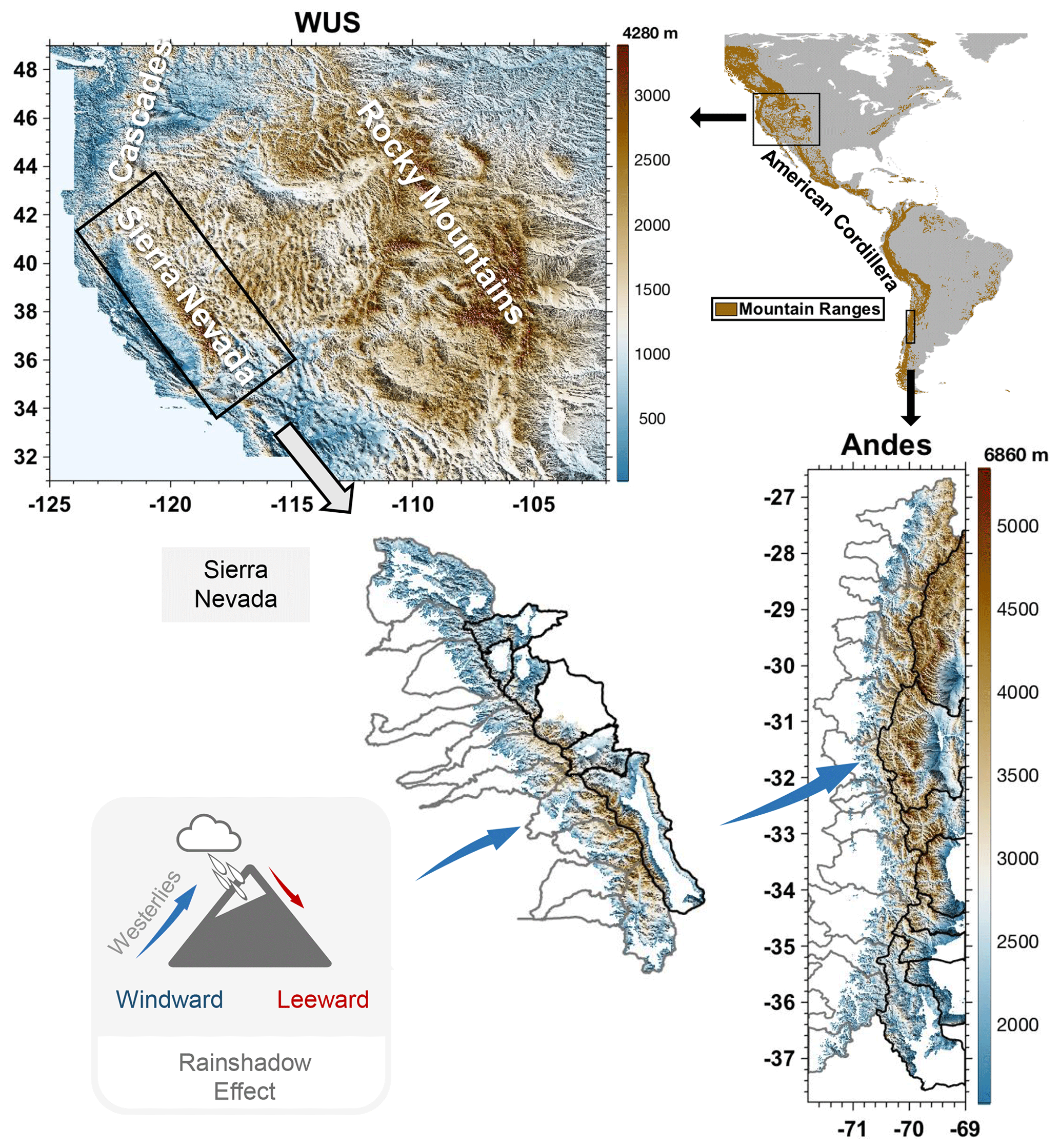
Figure 1DEM and location of midlatitude American Cordillera including its subdomains in the Western United States (WUS) and Andes. Bottom left cartoon highlights the typical rain shadow effect whereby moist air rises on the windward side of a mountain depositing significant amounts of snow, and drier air flows down the leeward side of the mountain creating a rain shadow effect. Arrows represent the generalized directions of westerlies that drive orographic and rain shadow SWE patterns. The Sierra Nevada (SN, sub-basin of WUS) and Andes are chosen to study the rain shadow effect. Windward watersheds are shown in gray boundaries, and leeward watersheds are shown in black boundaries. Mountain ranges are based on Snethlage et al. (2022).
The WUS contains three major mountain ranges including the Sierra Nevada, the Rocky Mountains, and the Cascades (Fig. 1). Amongst these, the Sierra Nevada subdomain is the closest analog to the Andes, sharing similar hydroclimatology and topography. Winter westerlies dominate precipitation timing and patterns in these two mountain ranges, leading to orographic gradients on the windward side of the mountains and rain shadow effects resulting in significant snow differences across relatively short windward–leeward gradients.
2.2 Datasets
This paper intercompares data from the Andes Snow Reanalysis (Andes-SR) and WUS Snow Reanalysis (WUS-SR) datasets (as reference datasets) to seven global snow datasets (available over both domains) and two regional datasets (available only over the WUS domain) shown in Table 1. The Andes-SR (WYs 1985 to 2015; Cortés and Margulis, 2017) SWE estimates were derived at a regular 180 m resolution grid before regridding to a regular latitude–longitude grid (0.001∘ or ∼100 m). The WUS-SR (WYs 1985 to 2021; Fang et al., 2022a) SWE estimates are at ∼480 m resolution. The different resolutions used for the Andes and WUS domains were based on computational constraints. In addition to spatial resolution differences, glaciers and elevation below 1500 m were masked out before applying the Andes-SR. The newer WUS-SR dataset is applied over the full domain and then masked afterwards as described in Fang et al. (2022a). The Andes-SR and WUS-SR datasets were both generated from the Bayesian framework developed by Margulis et al. (2016, 2019) with assimilation of fractional snow-covered area images derived from Landsat 5, 7, and 8 using a particle batch smoother (PBS; Margulis et al., 2015). Independent verification shows that both datasets are consistent with in situ peak SWE with a correlation coefficient of 0.73 over the Andes (Cortés and Margulis, 2017) and 0.77 (using >25 000 station years of in situ data) over the WUS (Fang et al., 2022a). Further verification of the WUS-SR SWE against Airborne Snow Observatory (ASO) SWE estimates shows consistent performance between these two spatial products with correlation coefficients ranging from 0.75 to 0.91. With high consistency against point-scale in situ and spatially distributed airborne SWE estimates, as well as the high spatial resolutions specifically targeting mountainous domains, these two snow reanalysis datasets are used as reference SWE datasets to evaluate the snow storage of global and regional products over the WUS and Andes.
The seven global snow products include ECMWF Reanalysis v5 (ERA5)-Land, ERA5, MERRA2, and four Global Land Data Assimilation System (GLDAS)-2.1 products (GLDAS-NOAH at 0.25∘, GLDAS-NOAH at 1.0∘, GLDAS-VIC (Variable Infiltration Capacity) at 1.0∘, and GLDAS-CLSM (Catchment) at 1.0∘). The Snow Data Assimilation System (SNODAS) and University of Arizona (UA) products only cover the United States and therefore are not included in the Andes intercomparison. Following Liu et al. (2022), SWE, precipitation, and snowfall were collected from each of the seven global products, SNODAS, and UA (including PRISM precipitation (Daly et al., 1994) used in the UA product). Since the reference snow reanalysis datasets do not output precipitation and snowfall, only SWE is used for reference. For the purposes of analysis and discussion in this work, the products described above are classified by their spatial resolution. Specifically, reference datasets and those products with spatial resolution less than ∼1 km are deemed “high resolution” (HR: WUS-SR, Andes-SR, and SNODAS), those with spatial resolutions between ∼1 and ∼ 10 km are deemed “moderate resolution” (MR: UA, ERA5-Land), and those with spatial resolutions greater than ∼ 10 km are deemed “low resolution” (“LR”: ERA5, GLDAS subset). Globally and regionally available datasets are referred to as “products” to distinguish them from the reference “datasets”, i.e., WUS-SR and Andes-SR.
The snow reanalysis reference datasets are, by design, constrained by satellite snow cover observations using a data assimilation approach. However, not all the products are solely model-based. SNODAS uses in situ snow, airborne SWE from gamma radiation snow surveys, and satellite snow cover, and UA uses in situ SWE as inputs to constrain estimates. Although ERA5 assimilates snow depth, limited examples of these in situ measurements are used in the WUS and Andes. However, in the WUS, with its relatively high density of in situ meteorological sites, almost all products are based on models with meteorological forcings that include some in situ measurements. In contrast, due to limited in situ meteorological sites in the Andes, the quality of input forcings remains unclear, but it is likely more uncertain than over the WUS. More details on the snow products used herein are given in Table 1 and Appendix A.
Table 1Details of snow datasets and products used in this work. Note that SNODAS data in WY 2004 are not used due to quality issues cited in Webster and Fetterer (2004).
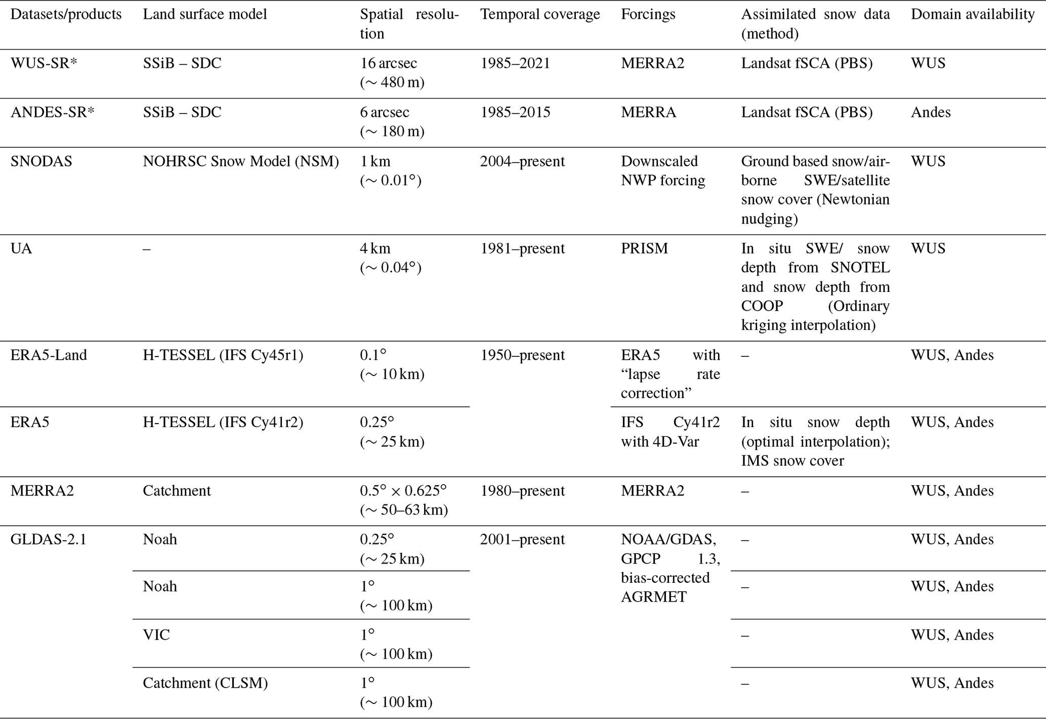
* Snow reanalysis datasets are used as reference datasets.
3.1 Intercomparison study period
Where possible, the intercomparison study periods in the two domains are chosen as WYs 1985–2021 (1 October 1984 to 30 September 2021) for the WUS, and WYs 1985–2015 (1 April 1984 to 31 March 2015) for the Andes, based on the availability of the respective snow reanalysis datasets. Among the products listed in Table 1, only GLDAS (starting in WY 2001) and SNODAS (starting in WY 2005) are not available over the full snow reanalysis period. For those products, long-term climatologies are necessarily derived over the shorter periods. Hence in the WUS, climatologies for the GLDAS and SNODAS products are over their available 21- and 17-year records, while all other products span the 37-year record. In the Andes, the GLDAS products are over their 15-year record, while all other products span the 31-year record. Analysis of climatological results from the products with longer periods does not show significant differences when applied to the shorter study periods (Fig. S1).
3.2 Focusing on intercomparison during the snow accumulation season
The intercomparison herein focuses on the snow accumulation season. To motivate this focus, the climatological (long-term average) daily time series of domain-aggregated SWE volume across all products are illustrated in Fig. 2. Two key points are evident: (i) there are significant discrepancies between products (which are analyzed in more detail below), and (ii) much of the uncertainty occurs during the accumulation season (and then propagates to the ablation season). An accurate characterization of peak SWE (at the end of the accumulation season) is a key metric of the final condition of snow accumulation processes and the initial condition leading into the main snowmelt season. Intercomparison of modeled snowmelt season processes is made more difficult when the initial conditions (i.e., peak SWE prior to the primary ablation season) across models are different. Given the large uncertainties observed in domain-wide peak SWE climatology (Fig. 2), this paper focuses on the uncertainties in the accumulation season (as done in Liu et al., 2022) in order to better understand how and why accumulation season estimates diverge across products. All the analyses focus on the accumulation season using metrics described below.
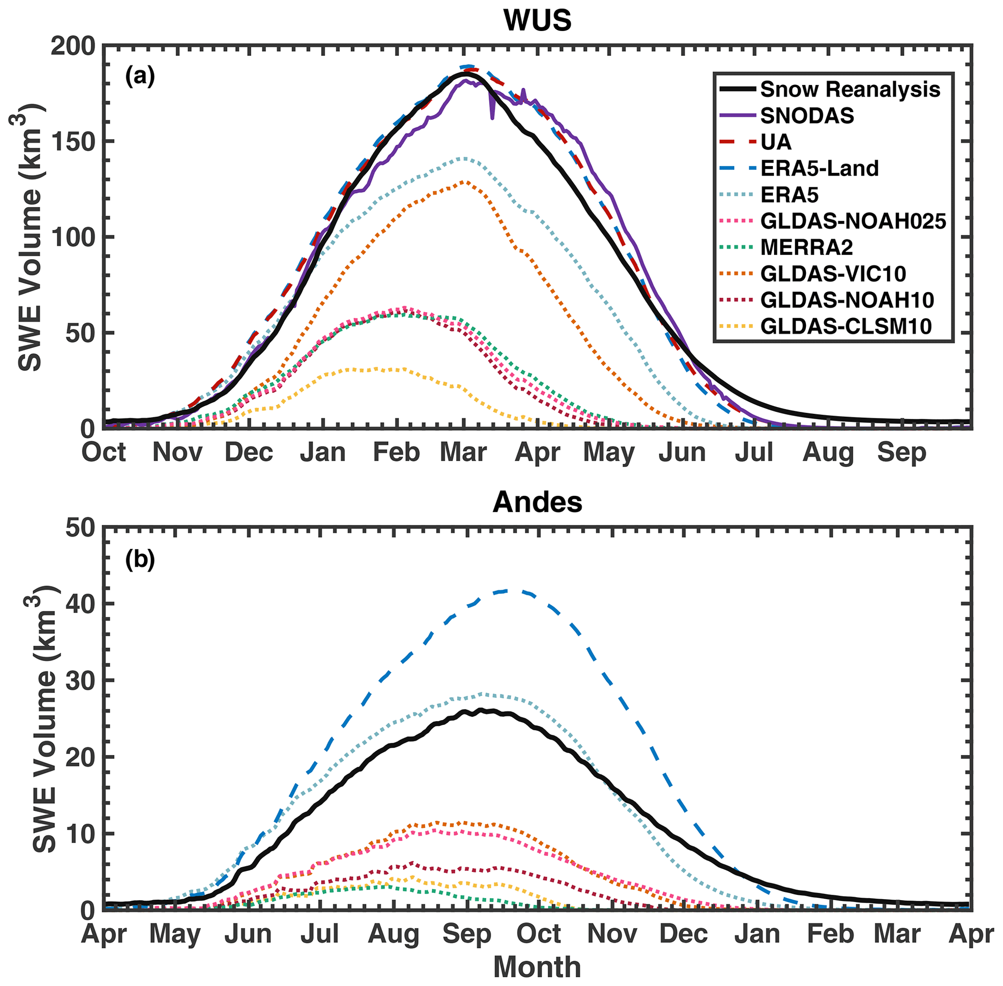
Figure 2Climatology of seasonal cycle of SWE volume in the WUS and Andes domains. Solid lines represent high-resolution (HR) datasets and products, dashed lines represent moderate-resolution (MR) products, and dotted lines represent low-resolution (LR) products.
3.3 Snow metrics used in the intercomparison
The processes leading to the domain-aggregated peak SWE shown in Fig. 2 depend on pixel-scale snow mass balance processes. Hereafter, for each product, the pixel-wise processes are analyzed prior to aggregating to the larger domain. The day corresponding to pixel-wise peak SWE (defined as tpeak) is computed for each product at their raw spatial resolution. The pixel-wise peak SWE depth (swepeak) is aggregated to get pixel-wise peak SWE volume (SWEpeak). Hence in results to follow, swepeak is used to describe and analyze maps of SWE, while SWEpeak is used to describe spatially aggregated volumes of SWE.
At each pixel, accumulation-season precipitation and snowfall are accumulated from the beginning of the WY up to tpeak, where the accumulated maps of SWE can then be aggregated over the domain of interest. The mass balance equations relating domain-aggregated cumulative snowfall (Sacc), SWE (SWEpeak), cumulative ablation (Aacc), cumulative precipitation (Pacc), cumulative snowfall (Sacc), and cumulative rainfall (Racc) are shown below:
where in Eqs. (1) and (2), Pacc, Sacc, and SWEpeak are directly computed from the snow products. Racc and Aacc are the residuals based on these two mass balance equations. Climatological values are computed as the long-term (interannual) mean of Pacc, Sacc, and SWEpeak over the intercomparison periods.
Persistent snow and ice areas are excluded before spatially integrating the SWE volumes, since most products analyzed in this work do not explicitly estimate glaciers and persistent snow. Such persistent snow and ice masks are first obtained from the Andes-SR and WUS-SR products and then aggregated to the spatial resolution of each product (as done in Liu et al., 2022). Domain masks in each product are also applied here, which are derived based on the reference datasets using the same approach. Details of persistent snow and ice masks and domain masks are described in Sect. S2 and shown in Figs. S2 and S3.
Beyond domain-wide results, we intercompare products and their ability to capture rain shadow effects, which often occur over short geographic scales but have significant influence on the water availability between windward and leeward sides of mountain ranges. For simplicity we focus on the windward–leeward contrasts over the Sierra Nevada in the WUS and those over the Andes. Figure 1 shows the boundaries of windward basins (in gray) and leeward basins (in black) for both domains. The Sierra Nevada and Andes are analogs of each other due to the mostly north–south orientation of the mountain ranges that are relatively perpendicular to the mostly westerly prevailing winds. In both cases, the windward and leeward basins serve distinct downstream populations, and so resolving those spatial variations has important hydrological implications. To assess the ability of products in capturing rain shadow effects, pixel-wise SWEpeak is aggregated over the windward () and leeward () watersheds. Since pixels may cover both windward and leeward watersheds, for MR and LR products, fractional swepeak is aggregated to get SWEpeak over the two types of watersheds separately (Figs. S4 and S5). For HR products and datasets, the pixels spanning the windward to leeward side have a negligible impact on the distribution. The fractional swepeak is computed by multiplying pixel-wise swepeak and the fraction of pixel within the windward or leeward watershed. The detailed steps used to derive the windward and leeward watershed snow storage are described in Sect. S3.
4.1 Climatological SWE uncertainty
4.1.1 Spatial distribution of pixel-wise peak SWE
Climatological pixel-wise swepeak maps for the WUS-SR (Fig. 3a) clearly show the highest snow storage occurring in the Sierra Nevada, the Cascades, and the Rocky Mountains. When integrated over the whole domain, the climatological WUS SWEpeak is 269 km3 (Fig. 3k). Similar spatial distributions of swepeak are observed for the HR (SNODAS; Fig. 3b) and MR products (UA and ERA5-Land; Fig. 3c and d). However, the remaining products (ERA5, MERRA5 and GLDAS subset; Fig. 3e to j) significantly underestimate swepeak and smooth out the spatial patterns captured by the HR and MR products. The combined HR and MR inter-product average of climatological WUS SWEpeak is 284±14 km3, in contrast to an average of 127±54 km3 for LR products (Fig. 3k). This suggests large uncertainty (both bias and spread) in SWEpeak among LR products. Compared to WUS-SR, SNODAS overestimates SWEpeak by ∼12 % (Fig. 3k) and exhibits higher swepeak in the Sierra Nevada, the Cascades, and the Rocky Mountains. UA and ERA5-Land both exhibit a similar magnitude of SWEpeak (differences <5 %) compared to WUS-SR, both of which have higher swepeak in the Cascades. Despite a similar spatial distribution of swepeak, ERA5 underestimates WUS SWEpeak by 22 % (Fig. 3k) compared to WUS-SR. All GLDAS products severely underestimate SWEpeak, where GLDAS-VIC10 shows the highest WUS SWEpeak (with a 35 % underestimation compared to WUS-SR).
Based on the Andes-SR, the climatological SWEpeak is 29 km3 (Fig. 4i). The southern Andes has higher swepeak compared to the northern region (Fig. 4a). The spatial distribution of swepeak and integrated SWEpeak volumes vary much more broadly across different products (Fig. 4b to k) in the Andes than they do in the WUS. The MR and LR inter-product average of climatological SWEpeak is 19±16 km3 (Fig. 4i). ERA5-Land and ERA5 overestimate SWEpeak by 66 % and 18 %, respectively (Fig. 4i). ERA5-Land significantly overestimates swepeak in the southern part of the Andes. Most of the LR products, including MERRA2 and the GLDAS subset, significantly underestimate SWEpeak by as much as 79 % (MERRA2), compared to Andes-SR (Fig. 4i). These findings for the Andes domain are qualitatively similar to Liu et al. (2022), where ERA5 and ERA5-Land overestimate SWEpeak and MERRA2 and GLDAS underestimate SWEpeak in High-Mountain Asia (HMA), another snow-dominated region with limited in situ measurements.
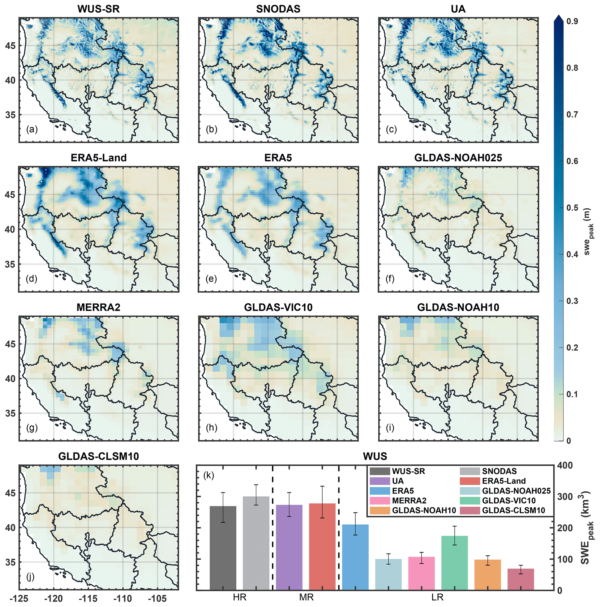
Figure 3(a–j) Spatial distribution of climatological swepeak in the WUS. Panel (k) shows the climatological WUS SWEpeak (colored bars) and the interannual interquartile range (IQR; black error bars). The bar plots are ordered by spatial resolution, with highest resolution on the left and lowest resolution on the right. The vertical dashed lines separate the three spatial resolution categories (i.e., HR km, ∼1 km < MR < ∼10 km, LR km). Glacier and permanent snow areas are masked out in the maps and domain-aggregated volumes.
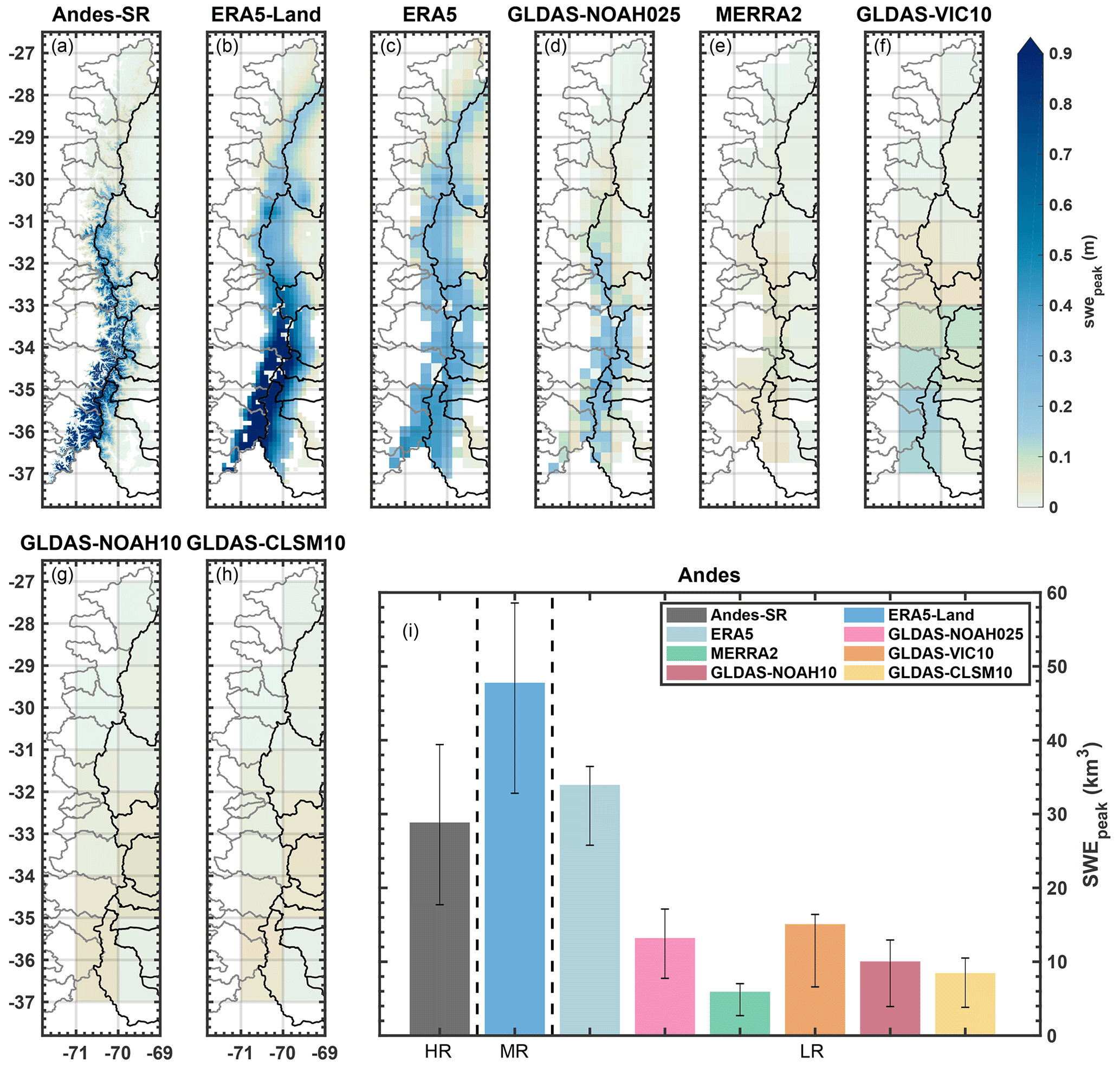
Figure 4(a–h) Spatial distribution of climatological swepeak in the Andes. Panel (i) shows the climatological Andes SWEpeak (colored bars) and the interannual interquartile range (IQR; black error bars). The bar plots are ordered by spatial resolution, with highest resolution on the left and lowest resolution on the right. The vertical dashed lines separate the three spatial resolution categories (i.e., HR km, ∼1 km < MR km, LR km). Glacier and permanent snow areas are masked out in the maps and domain-aggregated volumes.
4.1.2 Resolving key spatial gradients: rain shadow effects
In addition to the overall spatial distribution in SWE, the orographically driven rain shadow (windward vs. leeward) distribution represents an example of an important spatial feature in many mountain contexts. In mountain ranges exposed to persistent prevailing winds, it is expected that the windward side of the range will have more SWE than the leeward side (Fig. 1). While significant biases exist in products as described in Sect. 4.1.1, this section focuses on the relative patterns of windward vs. leeward storage. The differences in rain shadow storage gradients are specifically examined in the Sierra Nevada subdomain of the WUS and the Andes. While resolving rain shadow effects is challenging for narrow topographic regions like the Sierra Nevada and the Andes, it has important hydrological implications as large gradients in SWE storage propagate to spring/summer runoff and streamflow that supply downstream users.
Based on the WUS-SR in the Sierra Nevada (Fig. 5), the latitudinal distribution of is the largest in the 37–38∘ N latitudinal band, while the latitudinal distribution of is the largest in the 38–39∘ N latitudinal band. The latitudinal windward and leeward storage of SWE decreases monotonically north and south of these maximum values. The total stored windward volume is 3.74 times more than the leeward volume . This ratio is the combined effect of variations in area and SWE depth between the windward and leeward basins and identifies that (on average) the windward basins store between 3 and 4 times more SWE volume than the leeward basins. Given that the windward and leeward areas across which SWE is integrated are effectively the same across products, any differences in windward–leeward ratio are driven by differences in SWE depth. SWE depth variations are primarily driven by resolving orographic enhancement of snowfall between windward and leeward slopes. In the Sierra Nevada, only SNODAS and UA products (spatial resolutions km) exhibit comparable to ratios. The ratios of to are 4.20 (12 % greater than the WUS-SR) for SNODAS and 3.14 (16 % less than WUS-SR) for UA, suggesting a fairly good agreement between windward–leeward snow volume distributions in these products. However, resolving the pattern of windward–leeward snow distribution is significantly impaired in the other MR and LR products. The ratios computed from ERA5-Land, ERA5, GLDAS-NOAH025, MERRA2, GLDAS-VIC10, GLDAS-NOAH10, and GLDAS-CLSM10 range from 1.08–2.40 and are 36 %, 46 %, 43 %, 55 %, 68 %, 66 %, and 71 % less than that in the WUS-SR, respectively. Hence, the MR and LR products generally have too little snow on the windward side compared to the leeward side. The location of the windward maximum SWEpeak is consistent in most snow products with the exception of the LR products (i.e., ERA5, GLDAS), which have a secondary maximum between 39–40∘ N. The location of the leeward maximum SWEpeak is consistent in most of the snow products with the exception of MERRA2, which is maximum at a lower latitude.
Based on the Andes-SR, the largest is distributed in the 35–36∘ S latitudinal band, while the distribution of has two local maxima in the 31–32∘ S and 35–36∘ S latitudinal bands (Fig. 6). The ratio of to is 1.58 from the Andes-SR, which is again the combined effect of windward–leeward variations in both area and SWE depth. Like the Sierra Nevada, ERA5-Land and all of the LR products improperly partition SWEpeak over the windward vs. leeward basins in the Andes. These products have to ratios less than 1 indicating deficient snow in the windward watersheds compared to the leeward watersheds. The lowest to ratio of 0.72 is observed from MERRA2 (54 % less than Andes-SR). GLDAS-VIC10 has the largest to ratio of 0.92 among Andes global products, which is still 42 % less than the Andes-SR. For the windward watersheds, from ERA5-Land and GLDAS-CLSM10 are the highest in the same latitudinal band as the Andes-SR; however, the other products have an erroneous distribution. None of the products resolve the distribution on the leeward side.
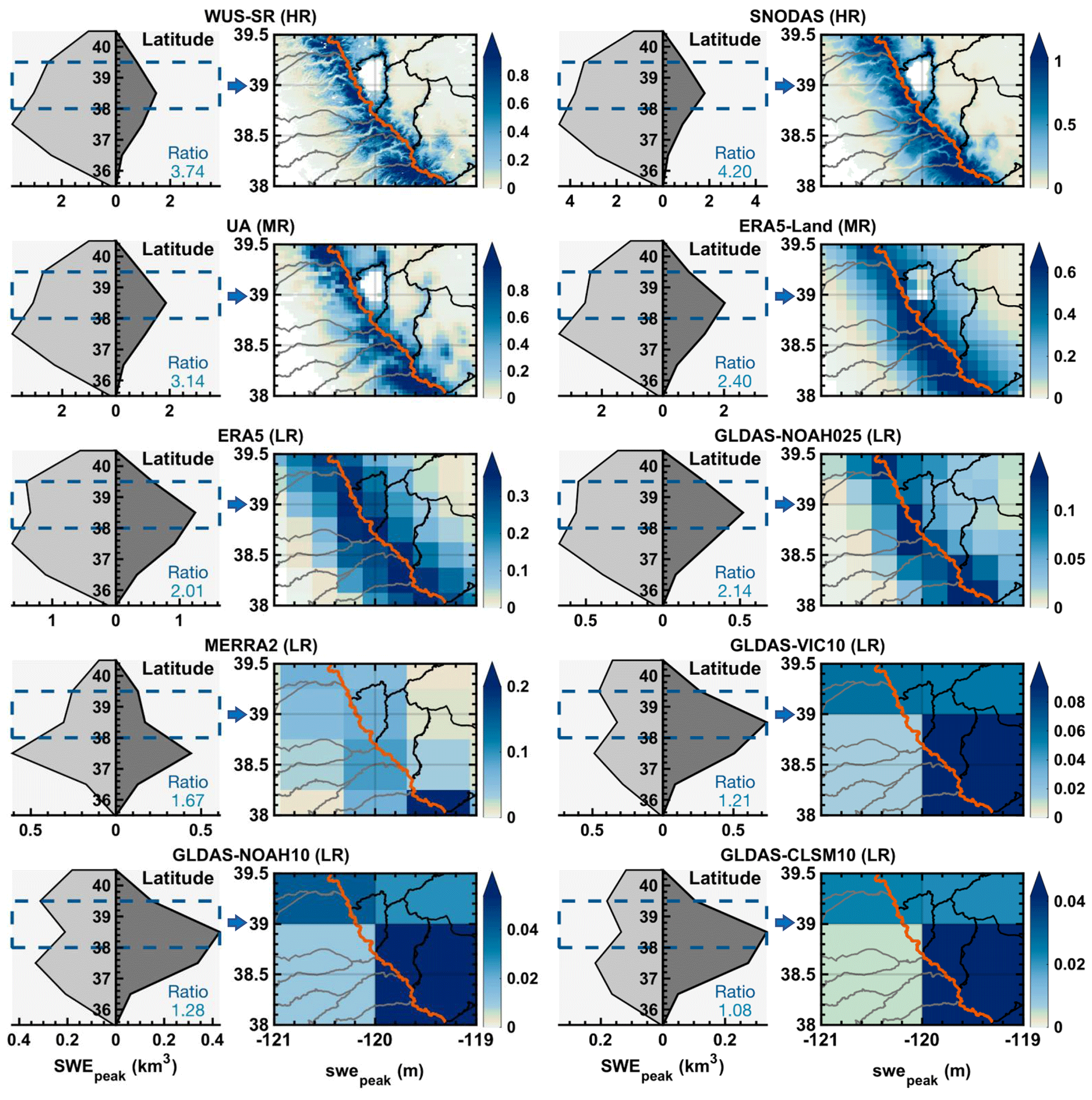
Figure 5Latitudinal distribution of integrated SWEpeak (km3) over windward (; light gray areas) and leeward basins (; dark gray areas) in the Sierra Nevada in first and third columns. Text labels indicate the ratio of latitudinally integrated to . The climatological swepeak (m) spatial patterns corresponding to the latitude bands indicated by dashed boxes are illustrated in the second and fourth columns. The red line represents the Sierra Nevada ridgeline separating windward (western) from leeward (eastern) basins. Note: different swepeak ranges are used for each product to highlight latitudinal/spatial patterns more than absolute values (due to significant biases in some products).
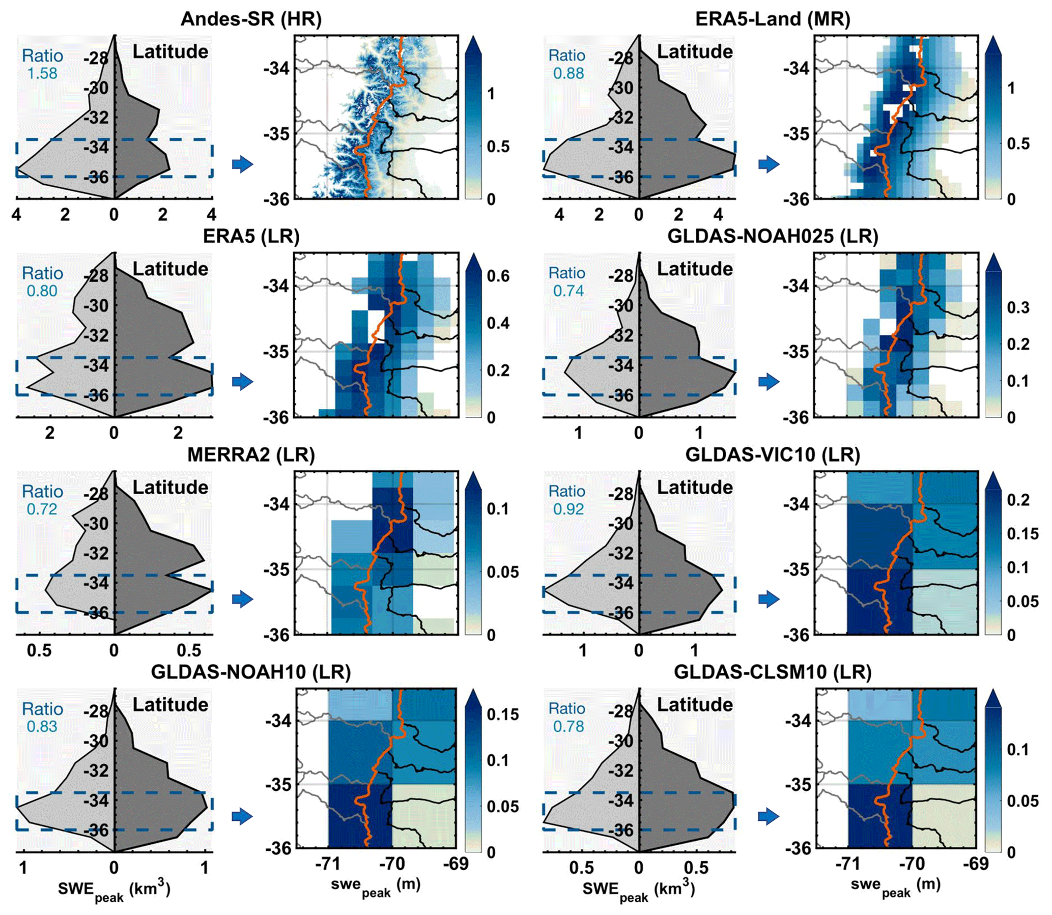
Figure 6Latitudinal distribution of SWEpeak (km3) over windward (; light gray areas) and leeward basins (; dark gray areas) in the Andes in first and third columns. Text labels indicate the ratios of latitudinally integrated to . The climatological swepeak (m) spatial patterns corresponding to the latitude bands indicated by dashed boxes are illustrated in the second and fourth columns. The red line represents the Andes ridgeline separating windward (western) from leeward (eastern) basins. Note: different swepeak ranges are used for each product to highlight latitudinal/spatial patterns.
The elevational distributions of bin-averaged climatological swepeak in the Sierra Nevada (Fig. 7a) and the Andes (Fig. 7b) are plotted to compare the elevational gradient of windward and leeward swepeak from products with different spatial resolutions. The lapse rate in swepeak was determined by linear regression of swepeak averaged across elevational bins (Sect. S5). Lapse rates from GLDAS products at 1.0∘ are not included because the subdomains analyzed are covered by fewer than 10 pixels (Figs. S7 and S8).
Based on the WUS-SR, climatological swepeak on the windward side of the Sierra Nevada monotonically increases up to ∼3.5 km. Across different products, the uncertainty of swepeak is smaller at the lower elevation ∼1–1.5 km; however, the differences in lapse rate project larger swepeak uncertainty as elevation increases. The gradients of windward swepeak (i.e., ) from WUS-SR, averaged over HR and MR products, and averaged over LR products are 0.34, 0.26, and 0.05 m km−1, respectively. On the leeward side of the Sierra Nevada, the swepeak increases monotonically with elevation from ∼1–3.5 km in the WUS-SR and most of the other products. Similarly, the uncertainty of swepeak is smaller at low elevation from ∼1–2 km and gradually increases with elevation corresponding with the differences in lapse rate across different products. The gradients of leeward swepeak (i.e., ) from WUS-SR, averaged over HR and MR products, and averaged over LR products are 0.21, 0.19, and 0.07 m km−1, respectively. HR and MR products have qualitatively similar elevational distributions of swepeak on both the leeward and windward side of the Sierra Nevada for elevations below 3 km, whereas those of swepeak from LR are underestimated with large differences in lapse rates compared to WUS-SR.
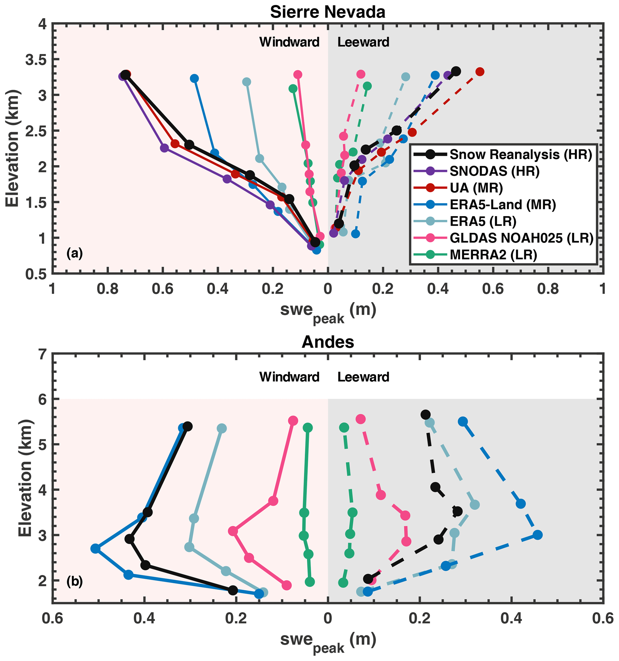
Figure 7Elevational distribution of windward and leeward swepeak in the Sierra Nevada (a) and the Andes (b) across reference datasets and products with spatial resolution higher than 1∘. Each dot represents the elevation bin-averaged swepeak. The number of pixels per bin is roughly equal. GLDAS products at 1∘ are not included for comparison due to too few points. On the windward side of the subdomains, dots within the red shaded areas are used to compute lapse rates. On the leeward side, dots in the darker shaded areas are used to compute lapse rates.
On the windward side of the Andes, swepeak from the Andes-SR increases from ∼1.5–3 km, with decreases between 3 and 6 km. The swepeak uncertainty is smaller at low elevation bands between ∼1.5–2 km. The uncertainty gets larger as elevation increases from 2–3 km corresponding to large differences in positive lapse rates. In contrast, large differences in negative lapse rates above 3 km reduce the uncertainty as elevation increases. The lapse rates of windward swepeak from the Andes-SR are 0.30 m km−1 between elevation bands of ∼1.5–3 km and −0.08 m km−1 between 3–6 km (Table S1). On the leeward side, swepeak increases between ∼1.5–3 km and slightly decreases above 3 km in the Andes-SR. Similar to the windward side, differences in positive lapse rate below 3 km project larger swepeak uncertainty as elevation increases from ∼1.5 km, whereas differences in negative lapse reduces uncertainty as elevation increases above 3 km. The lapse rates of leeward swepeak from the Andes-SR are 0.22 m km−1 between elevations of ∼1.5–3 km and −0.02 m km−1 between 3–6 km.
4.2 Interannual SWE uncertainty
The interannual variability of SWEpeak is in general agreement (with correlation coefficients R>0.85) between the WUS-SR snow reanalysis and other products shown in Fig. 8. SWEpeak from UA and ERA5-Land agrees well with WUS-SR in both magnitude and correlation (Fig. 8b and c), with relative mean differences (RMDs) of less than 3 % in absolute value and R>0.9. While SNODAS overestimates SWE volume with a RMD of 14 % (Fig. 8a), it shows consistent interannual variations with a high R value of 0.92. The LR products are generally well correlated with WUS-SR, although SWEpeak from these products is underestimated by as much as 190 km3 (GLDAS-CLSM10), equivalent to a RMD of 71 % compared to WUS-SR. Figure 8j shows that SWE percentiles computed from different products in the WUS are in better agreement in extreme years and in less agreement for near-average years. For example, WY 2017 was the wettest year among all products and WY 2015 was the driest year for all products except for SNODAS (in which WY 2005 is suspiciously low). WY 2014 was a normal-to-wet year with SWEpeak between the 60th and 70th percentiles from GLDAS-NOAH025, MERRA2, GLDAS-NOAH10, and GLDAS-CLSM10 but a normal-to-dry year with SWEpeak less than the 50th percentile in the other products.
The interannual variability of SWEpeak is in much less agreement in the Andes (Fig. 9; with R as low as 0.56). Figure 9 shows that ERA5-Land and MERRA2 are most consistent with Andes-SR in terms interannual variability (R>0.85). However, ERA5-Land overestimates SWEpeak by 18 km3 (RMD = 65 %), and MERRA2 underestimates SWEpeak by 23 km3 (RMD = −80 %). Although ERA5 has the smallest RMD of 17 %, the correlation coefficient R is 0.74, suggesting that SWEpeak from ERA5 is less representative of interannual variation in the Andes. For the GLDAS products, GLDAS-NOAH025 has R=0.79, whereas R values for other GLDAS products at 1∘ are less than 0.65, indicating that SWE from these LR products are less consistent with the interannual variation from Andes-SR. Figure 9a illustrates that the SWEpeak percentiles computed from the common 12-year record are much less consistent in the Andes than in the WUS (shown in Fig. 8j) for both normal and extreme years. Despite good temporal correlation of SWEpeak (R>0.86) in WUS, the relatively poorer temporal correlations (R>0.56) identified from the LR products in the Andes indicate that they may be less suitable for trend or other analyses that require snow estimates with representative interannual variability.
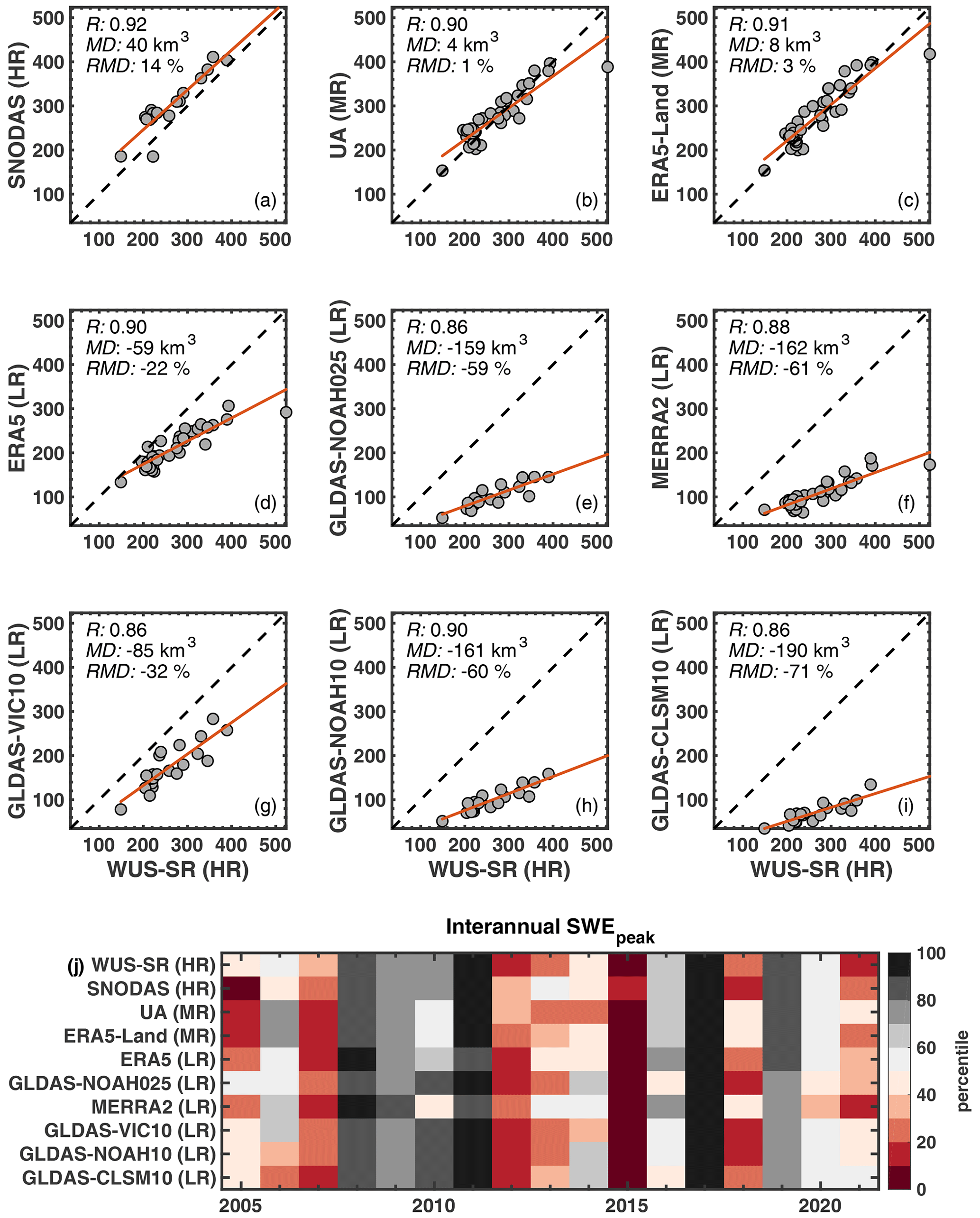
Figure 8Scatter plots (a–i) of SWEpeak volumes between WUS-SR and other products. Each dot represents SWEpeak volume (km3) for each year over the study period (WYs 1985 to 2021) where data are available. For the SNODAS and GLDAS products, the comparison is over WYs 2005 to 2021 and 2001 to 2021, respectively. The WY 1993 SWEpeak in WUS-SR is the highest and much higher than those from UA and ERA5-Land. Statistics do not change significantly if this data point is excluded. Panel (j) shows the SWEpeak percentiles in each WY over the overlapping period including all products (WYs 2005 to 2021).
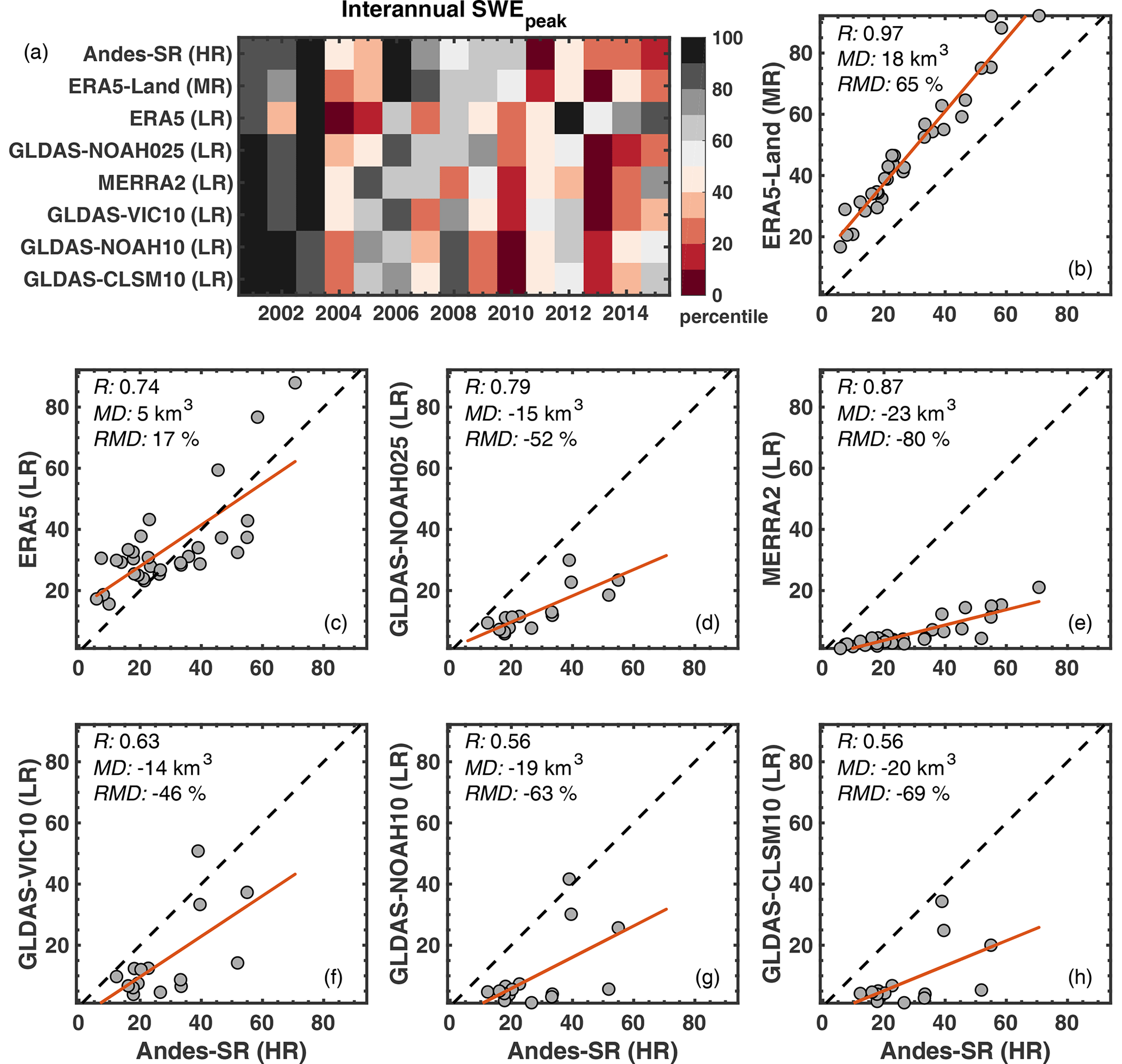
Figure 9Scatter plots (b–h) of SWEpeak volumes between Andes-SR and other products. Each dot represents SWEpeak volume (km3) for each year over the study period (WYs 1985 to 2015) where data are available. For the GLDAS products, the comparison is over WYs 2001 to 2015. Panel (a) shows the SWEpeak percentiles in each WY over the overlapping period including all products (WYs 2001 to 2015).
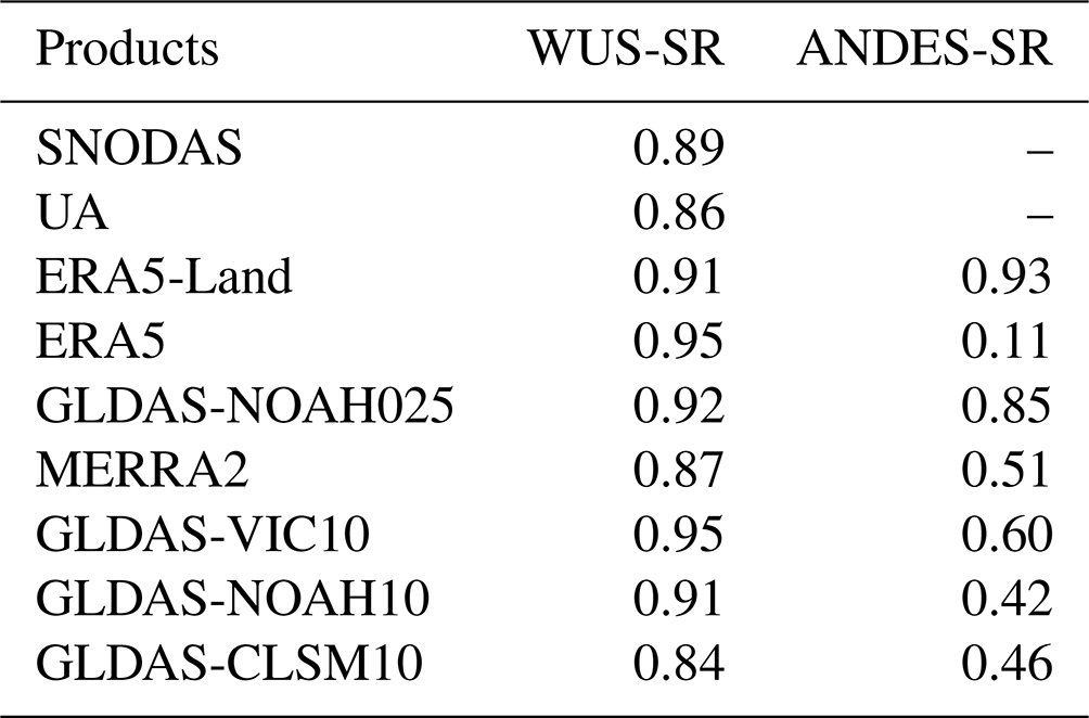
Overall, dry to wet years identified from products in the WUS generally agree with the WUS-SR with a correlation coefficient above 0.8 over WYs 2005 to 2021 (Table 2). In contrast, discrepancies are evident among SWEpeak percentiles computed from different products over WYs 2001 to 2021. Percentiles from ERA5-Land and GLDAS-NOAH025 agree well with the Andes-SR. However, the correlation is low between other products and Andes-SR. Although SWEpeak from ERA5 has comparable climatology with Andes-SR (Fig. 4i), its interannual distribution disagrees with the Andes-SR, especially after WY 2001.
Table 2Correlation of SWEpeak percentiles of each product against the reference datasets over WYs 2005 to 2021 in the WUS and WYs 2001 to 2021 in the Andes.
4.3 Drivers of SWE uncertainty
4.3.1 Impact of accumulation-season precipitation and snowfall on annual SWEpeak
To better understand the accumulation-season SWEpeak uncertainty driven by model inputs, the relationship among Pacc, Sacc, and SWEpeak is quantified for all products. The annual data points are more clustered in the WUS (Fig. 10a, b) than those in the Andes (Fig. 10c, d). GLDAS-CLSM10 and MERRA2 tend to have lower Pacc, Sacc and therefore SWEpeak in both the WUS and Andes. ERA5-Land and ERA5, on the other hand, have higher Pacc, Sacc, and SWEpeak in both domains. For rain–snow partitioning, UA (Fig. 10a) tends to have higher Sacc over the WUS compared to the other products. Given similar Sacc, SNODAS (Fig. 10b) is inclined to generate higher SWEpeak. In the Andes, GLDAS-NOAH10 and GLDAS-CLSM10 partition less Pacc into Sacc (circles lower than the regression line), in contrast to ERA5-Land and ERA5 that tend to partition more (Fig. 10c). SWEpeak from ERA5-Land diverges from ERA5 (Fig. 10d) given a similar amount of Pacc and Sacc, presumably caused by different melt amounts between the two products driven by resolution-induced elevation differences.
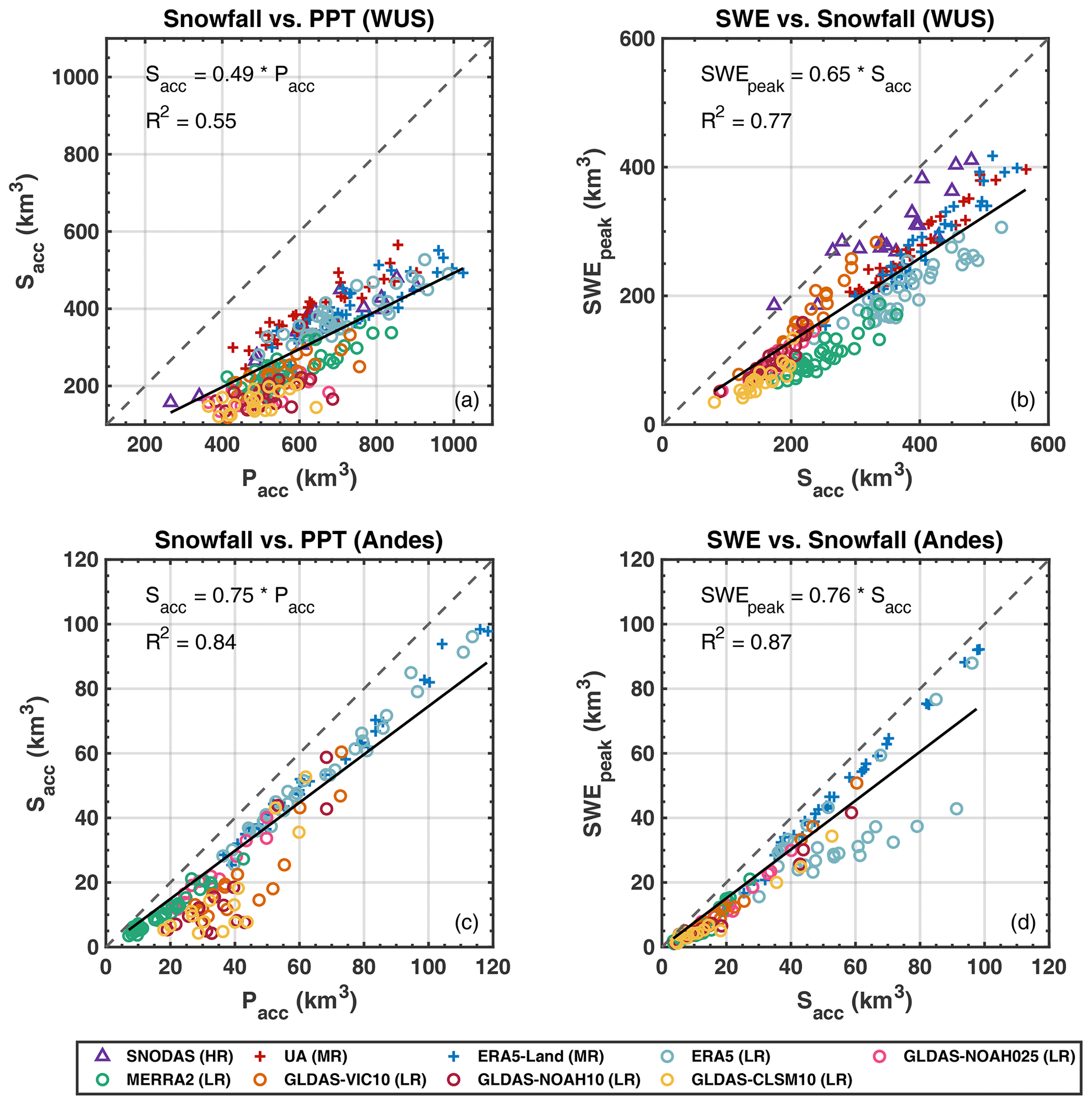
Figure 10Panels (a) and (c) show scatter plots of accumulation-season Sacc (km3) vs. Pacc (km3) volumes over the WUS and Andes, respectively, indicating the partitioning of precipitation into snowfall. Panels (b) and (d) show scatter plots of accumulation-season SWEpeak (km3) vs. Sacc (km3) over WUS and Andes, respectively, indicating how much snowfall remains as SWE vs. being lost to ablation. Solid lines are linear regression, and dashed lines are 1:1 lines.
Annual values of Pacc and Sacc estimates from all products show that the variance in Pacc explains the majority of the variance in snowfall in the accumulation season with a coefficient of determination R2=0.55 in the WUS (Fig. 10a) and R2=0.84 in the Andes (Fig. 10c). This is consistent with previous findings (Cho et al., 2022; Broxton et al., 2016b; Liu et al., 2022) and the expectation that precipitation is the major contributor to uncertainty in SWE. The lower R2 in the WUS compared to the Andes suggests that other factors such as air temperature plays a more important role in rain–snow partitioning in the WUS. Approximately 49 % of Pacc falls as snow in the WUS, whereas around 75 % of Pacc falls as snow in the Andes (Fig. 10a, c). This is because the Andes are at higher average elevation (∼2999 m) with cooler temperature than the WUS (∼1383 m), leading to more precipitation falling as snow. The variance in SWEpeak is mostly explained by the variance in Sacc, i.e., R2=0.77 in WUS (Fig. 10b) and R2=0.87 in the Andes (Fig. 10d). As a fraction of cumulative snowfall, 65 % and 76 % remain as SWEpeak in the WUS and Andes, respectively, while the rest is lost to accumulation-season ablation.
4.3.2 Impact of LSM and spatial resolution on climatological SWEpeak
To understand the impact of varying LSM mechanisms (i.e., rain–snow partitioning and snowmelt generation) and spatial resolution on the uncertainties in SWE, the climatological precipitation, snowfall, and SWEpeak for all products over the WUS and Andes are shown in Fig. 11. The rainfall to precipitation ratio (, gray text) represents the impact of rain–snow partitioning mechanisms, and the ablation to snowfall ratio (, black text) represents the impact of accumulation-season snowmelt mechanisms. It should be noted that different peak SWE days may impact via the accumulation window; i.e., the shorter accumulation season in the GLDAS subset (associated with earlier peak SWE days, tpeak, Fig. 11 red symbol) has cooler average temperature and thus lower . However, no significant relationship was found between tpeak and , suggesting that is not sensitive to tpeak. The WUS, with relatively lower elevation, has higher precipitation in the form of rainfall and higher snowfall loss to ablation than the Andes at higher elevation. In the WUS, ranges from 0.39 (UA) to 0.69 (GLDAS-CLSM10), and ranges from 0.15 (SNODAS) to 0.56 (MERRA2). In the Andes, ranges from 0.19 (ERA5-Land) to 0.57 (GLDAS-CLSM10), and ranges from 0.13 (ERA5-Land) to 0.48 (GLDAS-CLSM10). Precipitation tends to fall more as snow in the HR, MR, and ERA5 products, whereas a higher fraction of precipitation falls as rainfall in the other products (GLDAS, MERRA2), even though lower Pacc is observed in both domains. The differences in melt mechanisms across product models further differentiate the and therefore SWEpeak.
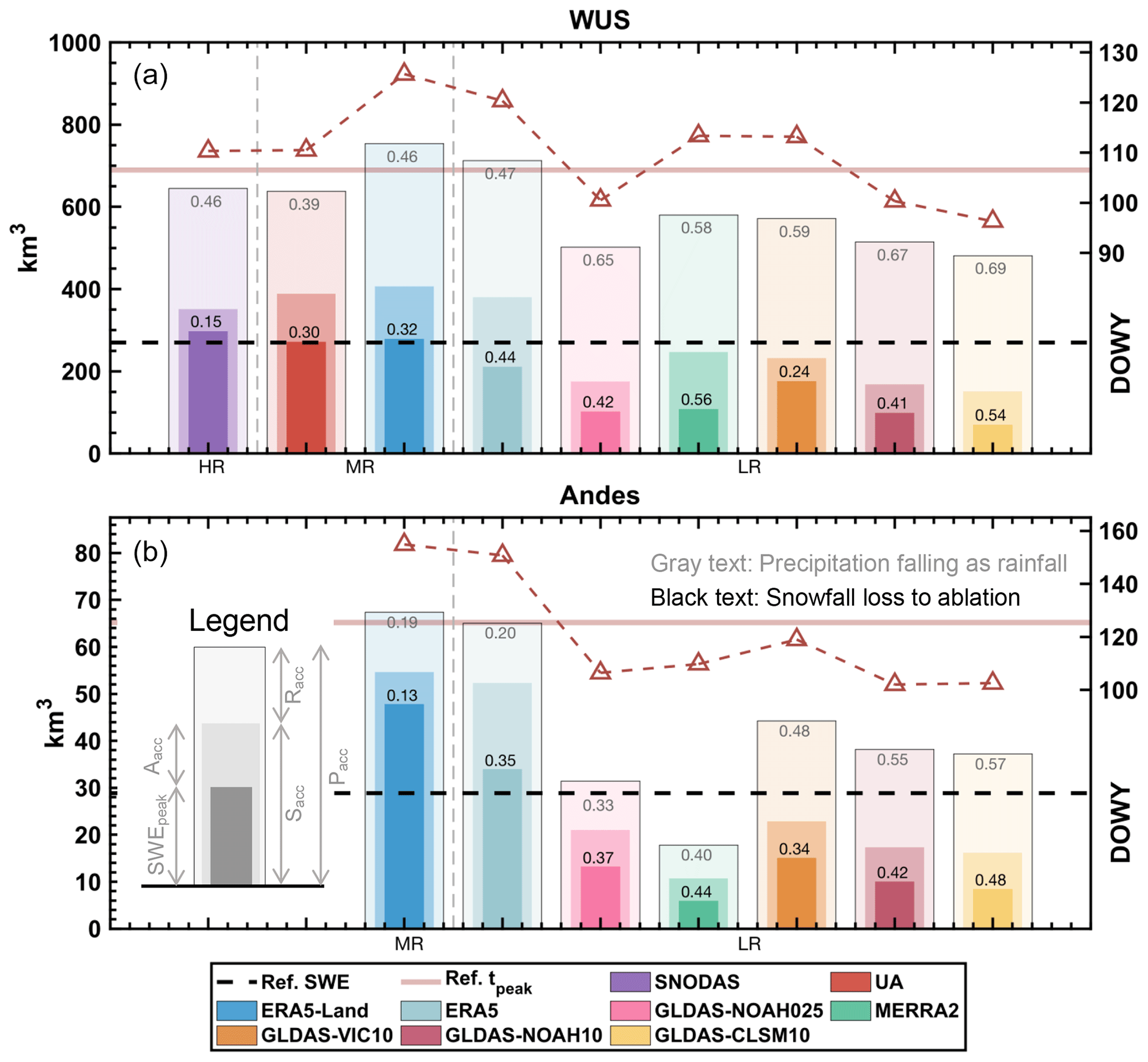
Figure 11Climatological SWEpeak, Sacc, and Pacc volumes aggregated over WUS (a) and the Andes (b) (in km3). Red triangles (corresponding to right y axis) show the tpeak averaged over all pixels and WYs. The horizontal dashed lines and red lines are the reference snow reanalysis SWE volumes and tpeak, respectively, from WUS-SR and Andes-SR. The vertical dashed lines group the products by spatial resolution (i.e., HR, MR, LR). The black text lists the , and gray text lists the .
Accumulation-season snowfall and SWEpeak are sensitive to different rain–snow partitioning and snowmelt generation mechanisms across products. The same precipitation inputs (with only minor differences caused by downscaling) are used to derive GLDAS estimates at 1.0∘ from three different LSMs, making the GLDAS models a useful subset to understand the impact of LSM process representation on SWE estimates. Among the GLDAS subset at 1.0∘, and range from 0.59–0.69 and 0.24–0.54, respectively, in the WUS (Fig. 12a), and range from 0.48–0.57 and 0.34–0.48, respectively, in the Andes (Fig. 12b). Compared to , a wider range of values are observed in both the WUS and Andes, suggesting that snowmelt generation mechanism differences contribute more to the climatological SWEpeak uncertainties than the rain–snow partitioning differences. Given a similar amount of Pacc, GLDAS-VIC10 partitions the most into snowfall even with later peak days, whereas GLDAS-CLSM10 partitions the least in both domains. The differences in are ≤0.1 between GLDAS-VIC10 and GLDAS-CLSM10 in contrast to the differences of 0.2–0.3 in . GLDAS-VIC10 tends to have higher Pacc, Sacc, and SWEpeak, which are closer to those from the HR or MR snow products. The better performance of GLDAS-VIC10 than others might be associated with the usage of snow elevational bands in the VIC model, in which sub-grid snowfall and SWE estimates are better represented. GLDAS-CLSM10 has the highest rates of and the lowest SWEpeak. A previous study shows a larger portion of snowfall is lost as accumulation-season ablation in the Catchment model (Xiao et al., 2021). Therefore, a better characterization of snowmelt during the accumulation season is beneficial to improve SWEpeak accuracy.
Domains with larger variance in elevation are likely to be more sensitive to model spatial resolution and therefore impact elevation-dependent mechanisms in the LSMs. ERA5-Land (0.1∘) and ERA5 (0.25∘) SWE are derived from the same LSM driven by similar forcings but modeled at different spatial resolutions. Similarly, GLDAS-NOAH025 (0.25∘) and GLDAS-NOAH10 (1∘) SWE are derived from the same Noah model driven by similar forcings but at two spatial resolutions. These two groups of products (Fig. 12c to f) are useful to isolate the impact of spatial resolution on SWE estimates via differences in elevation representation. The raw DEMs from each product are used to compute the mean and standard deviation of elevation over WUS and Andes. The Andes, located at higher elevation, also has a larger variance in elevation (standard deviation >1100 m) compared to the WUS (standard deviation <800 m) for any resolution. The standard deviation varies more significantly with resolution than the mean in both WUS and Andes (Fig. 12g, h). With coarser spatial resolution, the variance in elevation decreases, indicating that coarse-resolution products tend to underestimate the true variance in elevation. The differences in elevation variance between products are larger in the Andes than the WUS. For example, when increasing resolution of GLDAS from 1.0∘ (∼100 km) to 0.25∘ (∼25 km), the standard deviation of elevation increases by 14 % in the Andes compared to 8 % in the WUS. The is similar in the ERA5-Land and ERA5 for the same domains (i.e., 0.46 from ERA5-Land and 0.47 from ERA5 in the WUS; 0.19 from ERA5-Land and 0.20 from ERA5 in the Andes), suggesting that the rain–snow partitioning in the ERA5 models is relatively insensitive to the elevation differences introduced by different spatial resolutions. The Andes are located at a higher elevation than the WUS, resulting in lower . However, the varies significantly between ERA5-Land and ERA5 in both WUS (0.32 vs. 0.44, respectively) and Andes (0.13 vs. 0.35, respectively). Hence, even though similar amounts of snowfall are generated for ERA5 and ERA5-Land, SWEpeak can be significantly different due to differences in ablation resulting from spatial resolution-based elevation differences. For GLDAS-NOAH025 and GLDAS-NOAH10, and are similar in the WUS. Large differences of both and are observed between GLDAS-NOAH025 and GLDAS-NOAH10. This suggests that increasing spatial resolution from 0.25 to 0.1∘ (ERA5 subsets) significantly impacts snowmelt generation in both Andes and WUS, whereas increasing spatial resolution from to 1 to 0.25∘ (GLDAS subsets) impacts rain–snow partition and snowmelt generation only in Andes with its larger differences in standard deviation of elevation between products at two different spatial resolutions.
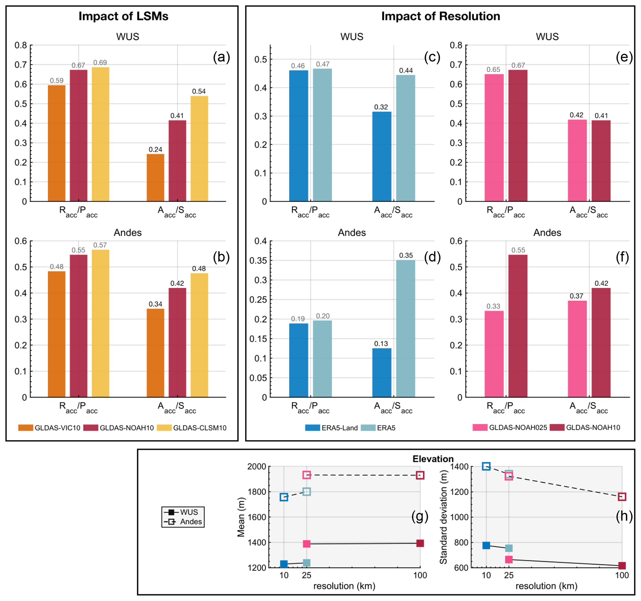
Figure 12(a, b) and for three GLDAS LSMs (VIC, Noah, and Catchment) at the same spatial resolution (∼100 km). (c, d) and for ERA5-Land (∼10 km) and ERA5 (∼25 km) using the same LSM and similar forcings, but different spatial resolutions. (e, f) and for GLDAS-NOAH025 (∼25 km) and GLDAS-NOAH10 (∼100 km) using the same LSM and similar forcings, but different spatial resolutions. (g, h) Mean and standard deviation of elevation over WUS and Andes from the ERA5-Land and ERA5 group and the GLDAS-NOAH025 and GLDAS-NOAH10 group (where colors represent the products shown in (c–f)).
This paper quantifies the spatiotemporal snow storage uncertainty over the midlatitude American Cordillera (i.e., the intermountain WUS and Andes) that is influenced significantly by snow processes. These two domains are both snow-dominated areas sharing similar hydrometeorology; however, a lot fewer in situ measurements are available in the Andes compared with the WUS. The uncertainties of snow water storage, spatial patterns (including orographic and rain shadow effect), and interannual variability are analyzed among the high-resolution (HR, less than ∼1 km), moderate-resolution (MR, between ∼1 to ∼10 km) and low-resolution (LR, greater than ∼10 km) snow products. The impact of forcings, LSM differences, and spatial resolution on snow storage uncertainty is assessed to provide insights for generating future snow products, especially for snow-dominated regions including areas with scarce in situ measurements.
With respect to characterizing climatological and interannual storage uncertainty, the key conclusions are the following:
-
In the WUS, HR and MR snow products are in better agreement with WUS-SR peak snow storage (269 km3) than the LR snow products, where the snow storage is biased low with large uncertainty. The climatological snow storage was found to be 284±14 km3 among HR and MR products and 127±54 km3 among LR products. For context, the reservoir capacity in the contiguous United States is around 600 km3 (Steyaert et al., 2022). Thus, based on the WUS-SR, the snow water stored in the WUS is 45 % (269 km3 of WUS-SR SWE km3 of contiguous US reservoir capacity) of the total reservoir capacity. Compared to the snow storage from WUS-SR, the averaged snow water storage from LR products misses 142 km3 of snow water storage, equivalent to 24 % of total reservoir capacity over the contiguous United States. In the Andes, MR and LR products exhibit much larger relative uncertainty in snow storage. The Andes-wide peak snow storage estimates are less clustered by spatial resolution with climatological estimates of 19±16 km3 compared with peak snow storage of 29 km3 from Andes-SR. The averaged SWE volumes from LR products in the WUS and Andes are underestimated by over 30 % compared to the reanalysis datasets. For similar melt rates, SWE computed from LR models would therefore disappear more quickly than HR/MR products. Hence calculation of snow volume sensitivity based on LR products could exaggerate the impact of warming on snow loss.
-
Beyond significant biases in overall storage, most of the global products poorly characterize snow storage variations related to orographically induced rain shadow effects. Compared to the WUS-SR, only SNODAS (spatial resolution of ∼1 km) and UA (∼4 km) reasonably distribute snow storage over windward and leeward watersheds in the Sierra Nevada. Globally available MR and LR products partition less snow storage on the windward side in both the Sierra Nevada and the Andes. In the Andes, global products show that more snow water is stored on the leeward side of the mountain than the windward side, completely missing the orographic and rain shadow patterns. Based on these results, to accurately resolve topographically driven features in snow storage likely requires spatial resolutions less than ∼5 km.
-
Consistent interannual variability is observed among all products assessed in the WUS, whereas there is less agreement in the Andes. This suggests that snow trend studies based on these globally availably snow products applied in the Andes might not be as reliable as those applied in the WUS.
With respect to drivers of uncertainty in snow storage estimates, the key conclusions are as follows:
-
Precipitation primarily explains the variance of snowfall as expected, which propagates to the variance of snow storage. Precipitation uncertainty accounts for a larger portion of snowfall uncertainty in the Andes than the WUS.
-
Aside from precipitation, LSM differences result in varying rain–snow partitioning and snowmelt generation, which play important roles in snow storage variance. Accumulation-season snowmelt generation mechanisms tend to contribute more to the climatological SWEpeak uncertainties than the rain–snow partitioning. At coarser spatial resolutions, there is a larger spatial variance in elevation between products in the Andes that propagates to larger differences in precipitation falling as rainfall, snowfall loss to ablation, and thus SWEpeak than in the WUS where elevation variance is lower.
Data assimilation techniques are used to constrain the SWE uncertainties in SNODAS, UA, WUS-SR, and Andes-SR. Moreover, many products are implicitly constrained by their use of in situ precipitation data in some form over the WUS. With more accurate precipitation estimates in the WUS, products at HR to MR show reasonable estimates of SWEpeak. However, ERA5-Land (MR) and LR products miss orographic and rain shadow patterns (Sect. 4.1.2). SNODAS and UA generate high-quality SWE estimates in the WUS via inclusion of in situ SWE measurements that are generally unavailable for regions like the Andes. Additionally, regions like Andes do not have sufficient in situ forcing measurements, resulting in a large uncertainty in forcings that propagates to SWE.
Although HR and MR products reasonably estimate snow storage in the WUS, uncertainty in snow storage from products at coarse spatial resolution in the WUS and at moderate and coarse spatial resolution in the Andes (where there are limited in situ measurements) needs to be reduced to increase their utility for understanding the role of snow in regional water and energy cycling. Resolving orographic and rain shadow patterns is still a challenging task among existing products. Future work is needed to reduce the accumulation-season snow storage uncertainty for mountainous regions with limited in situ measurements. Beyond the accumulation-season processes focused on herein, the snowmelt uncertainty and its drivers in the melt-season should be investigated to further characterize additional uncertainty in warm-season snowmelt rates and timing. New and future SWE products such as the recently published SWE reconstruction at 500 m (Bair et al., 2023) and other products such as Daymet SWE at 1 km (Thornton et al., 2021) could be examined to further characterize uncertainty in higher-resolution products. The ability to capture orographic and rain shadow patterns from snow reanalysis datasets and SNODAS encourages the usage of existing spaceborne snow-covered area measurements and/or future spaceborne missions that can directly provide high-resolution SWE measurements to constrain mountain SWE.
A1 HR product
SNODAS (Webster and Fetterer, 2004) outputs daily SWE from WY 2004 at 1 km over CONUS. Although SNODAS is available starting from WY 2004, data assimilation was only regularly performed from WY 2005. Therefore, it is suggested to exclude SNODAS data in WY 2004 for analysis. SNODAS SWE is generated the from NOHRSC Snow Model, an energy and mass balance model forced with downscaled forcings from numerical weather prediction (NWP) models. Assimilation of ground-based snow data, airborne SWE from gamma radiation snow surveys, and satellite snow cover is performed via Newtonian nudging.
A2 MR products
The UA daily SWE dataset (Zeng et al., 2018; Broxton et al., 2019) at 4 km over CONUS is generated from analysis and interpolation of in situ measurements including SWE from SNOTEL, snow depth, air temperature, and precipitation from COOP stations, and gridded estimates including air temperature and precipitation from PRISM. The ordinary kriging method is used for interpolating the ratio of SWE to net snowfall at in situ sites to the PRISM grid. The interpolated ratio is then multiplied by gridded 4 km PRISM net snowfall to get gridded SWE. At in situ sites, precipitation falls as snow on days when snow depth change is positive. As a result, snowfall may be overestimated on rain-on-snow days when both rainfall and snowfall occur, but precipitation is entirely recorded as snowfall. The temperature threshold to partition PRISM precipitation into snowfall and rainfall is interpolated from in situ threshold determined by each site (Broxton et al., 2016a, b). Net snowfall is estimated by the difference in accumulated snowfall and accumulated ablation, which is a function of degree days above 0 ∘C. A new snow density parameterization (Dawson et al., 2017) was developed to convert snow depth at COOP stations to SWE. Precipitation and air temperature for UA are taken from PRISM (Daly et al., 1994).
ERA5-Land (Muñoz-Sabater et al., 2021) hourly SWE globally at 0.1∘ is generated from the same land surface model as ERA5 (with different versions) but driven by downscaled and lapse rate corrected forcings from ERA5 at higher spatial resolution. Specifically, shortwave, longwave, liquid, and solid precipitation are downscaled using a linear triangular mesh interpolation. Other variables such as air temperature, specific humidity, relative humidity, and surface pressure are adjusted to account for differences in elevations between the two spatial resolutions. No additional data assimilation is involved in generating the ERA5-Land SWE.
A3 LR products
ERA5 (Hersbach et al., 2020) outputs hourly SWE globally at 0.25∘ using the H-TESSEL model. An optimal interpolation (OI) method is used to update the grid-averaged snow depth from a maximum of 50 in situ measurements within a radius of 250 km from a given grid cell. In situ snow depth observations from surface synoptic (SYNOP) and World Meteorological Organization Global Telecommunication System (GTS) are used as assimilated measurements, and 4 km snow extent from NOAA/National Environmental Satellite, Data and Information Service (NESDIS) has been applied at an elevation lower than 1500 m since 2004. However, SNOTEL/SCAN/COOP snow depths in the WUS are not currently used in the snow assimilation system. Though there might be some sparsely distributed in situ sites that measure snow depth which were assimilated in the WUS and Andes, the impact of data assimilation on SWE in both regions appears to be negligible. The binary snow extent is converted to snow depth at grids below 1500 m, assuming 5 cm of snow depth when snow cover is 100 %. The conversion is not conducted at elevations above 1500 m to avoid improper terrain information from coarse spatial resolution in mountainous areas. SWE is set to 10 m at permanent snow and ice grids. Beyond snow observations, 4 km precipitation data from National Centers for Environmental Prediction (NCEP) stage IV over the United States were assimilated in ERA5 using 4D-Var data assimilation method (Lopez, 2011). NCEP precipitation data are produced radar and gauge observations (Lin and Mitchell, 2005). Hence it is reasonable to assume that ERA5 precipitation may be more accurate over the WUS than the Andes, where such data are not assimilated.
The suite of GLDAS 2.1 products consist of daily SWE since WY 2001 from four globally distributed products (Rodell et al., 2004). The four products are generated from three LSMs and at two spatial resolutions (i.e., Noah LSM at 0.25∘: GLDAS – NOAH025; Noah LSM at 1.0∘: GLDAS – NOAH10; VIC LSM at 1.0∘; GLDAS – VIC10; Catchment LSM at 1.0∘: GLDAS – CLSM10). The same meteorological forcings from multiple sources, including NOAA/GDAS, GPCP1.3, and corrected AGRMET, are employed to generate the four products. Adjustments for forcings are conducted to account for the elevation differences between GLDAS at 1.0 and 0.25∘. No snow data assimilation is conducted in generating the products, whereas input forcings include sources from in situ measurements.
MERRA2 outputs hourly SWE globally at 0.625∘ × 0.5∘ resolution using the Catchment LSM (Reichle et al., 2017). The Catchment LSM is forced by bias-corrected precipitation using Climate Prediction Center (CPC) unified gauge-based analysis of global daily precipitation products. Similar to the GLDAS subset, no snow data assimilation is involved in generating the MERRA2 dataset, whereas in situ precipitation measurements are involved in deriving the SWE.
The Andes-SR and WUS-SR datasets are publicly available at https://doi.org/10.5061/dryad.ngf1vhj0s (Margulis and Fang, 2023) and https://doi.org/10.5067/PP7T2GBI52I2 (Fang et al., 2022b), respectively. The SNODAS product is available at https://doi.org/10.7265/N5TB14TC (National Operational Hydrologic Remote Sensing Center, 2004). The UA daily SWE product is available at https://doi.org/10.5067/0GGPB220EX6A (Broxton et al., 2019). The PRISM product is available at https://prism.oregonstate.edu (PRISM Climate Group, Oregon State University, 2014). The ERA5 product is available at https://doi.org/10.24381/cds.adbb2d47 (Hersbach et al., 2023). The ERA5-land product is available at https://doi.org/10.24381/cds.e2161bac (Muñoz Sabater, 2019). For GLDAS 2.1 products, the GLDAS–NOAH025 is available at https://doi.org/10.5067/E7TYRXPJKWOQ (Beaudoing and Rodell, 2020a); GLDAS–NOAH10 is available at https://doi.org/10.5067/IIG8FHR17DA9 (Beaudoing and Rodell, 2020b); GLDAS–VIC10 is available at https://doi.org/10.5067/ZOG6BCSE26HV (Beaudoing and Rodell, 2020c), and GLDAS–CLSM10 products are available at https://doi.org/10.5067/VCO8OCV72XO0 (Li et al., 2020). MERRA2 SWE is available at https://doi.org/10.5067/RKPHT8KC1Y1T (Global Modeling and Assimilation Office, 2015a); bias-corrected precipitation is available at https://doi.org/10.5067/7MCPBJ41Y0K6 (Global Modeling and Assimilation Office, 2015b); bias-corrected snowfall is available at https://doi.org/10.5067/L0T5GEG1NYFA (Global Modeling and Assimilation Office, 2015c).
The supplement related to this article is available online at: https://doi.org/10.5194/tc-17-5175-2023-supplement.
YF contributed to data acquisition and analysis, manuscript conceptualization, and writing. YL contributed to data acquisition, manuscript conceptualization, and revision. DL contributed to manuscript conceptualization and revision. HS contributed to manuscript conceptualization and revision. SAM contributed to manuscript conceptualization, revision, and supervision.
The contact author has declared that none of the authors has any competing interests.
Publisher's note: Copernicus Publications remains neutral with regard to jurisdictional claims made in the text, published maps, institutional affiliations, or any other geographical representation in this paper. While Copernicus Publications makes every effort to include appropriate place names, the final responsibility lies with the authors.
We thank Editor Edward Bair and two anonymous reviewers for their thorough and valuable comments on our manuscript.
This work is funded by the National Science Foundation (NSF) (grant no. 1641960), the National Oceanic and Atmospheric Administration (NOAA) OAR/OWAQ Observations Program (award no. NA18OAR4590396), and the National Aeronautics and Space Administration (NASA) IDS (grant no. 80NSSC20K1293).
This paper was edited by Edward Bair and reviewed by two anonymous referees.
Bair, E. H., Dozier, J., Rittger, K., Stillinger, T., Kleiber, W., and Davis, R. E.: How do tradeoffs in satellite spatial and temporal resolution impact snow water equivalent reconstruction?, The Cryosphere, 17, 2629–2643, https://doi.org/10.5194/tc-17-2629-2023, 2023.
Beaudoing, H. and Rodell, M.: NASA/GSFC/HSL (2020), GLDAS Noah Land Surface Model L4 3 hourly 0.25 × 0.25 degree V2.1, Greenbelt, Maryland, USA, Goddard Earth Sciences Data and Information Services Center (GES DISC) [data set], https://doi.org/10.5067/E7TYRXPJKWOQ, 2020a.
Beaudoing, H. and Rodell, M.: NASA/GSFC/HSL (2020), GLDAS Noah Land Surface Model L4 3 hourly 1.0 × 1.0 degree V2.1, Greenbelt, Maryland, USA, Goddard Earth Sciences Data and Information Services Center (GES DISC) [data set], https://doi.org/10.5067/IIG8FHR17DA9, 2020b.
Beaudoing, H. and Rodell, M.: NASA/GSFC/HSL (2020), GLDAS VIC Land Surface Model L4 3 hourly 1.0 × 1.0 degree V2.1, Greenbelt, Maryland, USA, Goddard Earth Sciences Data and Information Services Center (GES DISC) [data set], https://doi.org/10.5067/ZOG6BCSE26HV, 2020c.
Broxton, P., Zeng, X., and Dawson, N.: Daily 4 km Gridded SWE and Snow Depth from Assimilated In-Situ and Modeled Data over the Conterminous US, Version 1, Boulder, Colorado USA. NASA National Snow and Ice Data Center Distributed Active Archive Center [data set], https://doi.org/10.5067/0GGPB220EX6A, 2019.
Broxton, P. D., Dawson, N., and Zeng, X.: Linking snowfall and snow accumulation to generate spatial maps of SWE and snow depth, Earth Space Sci., 3, 246–256, https://doi.org/10.1002/2016EA000174, 2016a.
Broxton, P. D., Zeng, X., and Dawson, N.: Why Do Global Reanalyses and Land Data Assimilation Products Underestimate Snow Water Equivalent?, J. Hydrometeorol., 17, 2743–2761, https://doi.org/10.1175/JHM-D-16-0056.1, 2016b.
Cho, E., Vuyovich, C. M., Kumar, S. V., Wrzesien, M. L., Kim, R. S., and Jacobs, J. M.: Precipitation biases and snow physics limitations drive the uncertainties in macroscale modeled snow water equivalent, Hydrol. Earth Syst. Sci., 26, 5721–5735, https://doi.org/10.5194/hess-26-5721-2022, 2022.
Cortés, G. and Margulis, S.: Impacts of El Niño and La Niña on interannual snow accumulation in the Andes: Results from a high-resolution 31 year reanalysis, Geophys. Res. Lett., 44, 6859–6867, https://doi.org/10.1002/2017GL073826, 2017.
Daly, C.: Guidelines for assessing the suitability of spatial climate data sets, Int. J. Climatol., 26, 707–721, https://doi.org/10.1002/joc.1322, 2006.
Daly, C., Neilson, R. P., and Phillips, D. L.: A Statistical-Topographic Model for Mapping Climatological Precipitation over Mountainous Terrain, J. Appl. Meteorol. Climatol., 33, 140–158, https://doi.org/10.1175/1520-0450(1994)033<0140:ASTMFM>2.0.CO;2, 1994.
Dawson, N., Broxton, P., and Zeng, X.: A New Snow Density Parameterization for Land Data Initialization, J. Hydrometeorol., 18, 197–207, https://doi.org/10.1175/JHM-D-16-0166.1, 2017.
Dozier, J., Bair, E. H., and Davis, R. E.: Estimating the spatial distribution of snow water equivalent in the world's mountains, WIREs Water, 3, 461–474, https://doi.org/10.1002/wat2.1140, 2016.
Fang, Y., Liu, Y., and Margulis, S. A.: A western United States snow reanalysis dataset over the Landsat era from water years 1985 to 2021, Sci. Data, 9, 677, https://doi.org/10.1038/s41597-022-01768-7, 2022a.
Fang, Y., Liu, Y., and Margulis, S. A.: Western United States UCLA Daily Snow Reanalysis, Version 1, Boulder, Colorado USA. NASA National Snow and Ice Data Center Distributed Active Archive Center [data set], https://doi.org/10.5067/PP7T2GBI52I2, 2022b.
Global Modeling and Assimilation Office (GMAO): MERRA-2 tavg1_2d_lnd_Nx: 2d,1-Hourly,Time-Averaged,Single-Level,Assimilation,Land Surface Diagnostics V5.12.4, Greenbelt, MD, USA, Goddard Earth Sciences Data and Information Services Center (GES DISC) [data set], https://doi.org/10.5067/RKPHT8KC1Y1T, 2015a.
Global Modeling and Assimilation Office (GMAO): MERRA-2 tavg1_2d_flx_Nx: 2d,1-Hourly,Time-Averaged,Single-Level,Assimilation,Surface Flux Diagnostics V5.12.4, Greenbelt, MD, USA, Goddard Earth Sciences Data and Information Services Center (GES DISC) [data set], https://doi.org/10.5067/7MCPBJ41Y0K6, 2015b.
Global Modeling and Assimilation Office (GMAO): MERRA-2 tavg1_2d_lfo_Nx: 2d,1-Hourly,Time-Averaged,Single-Level,Assimilation,Land Surface Forcings V5.12.4, Greenbelt, MD, USA, Goddard Earth Sciences Data and Information Services Center (GES DISC), [data set], https://doi.org/10.5067/L0T5GEG1NYFA, 2015c.
Hersbach, H., Bell, B., Berrisford, P., Hirahara, S., Horányi, A., Muñoz-Sabater, J., Nicolas, J., Peubey, C., Radu, R., Schepers, D., Simmons, A., Soci, C., Abdalla, S., Abellan, X., Balsamo, G., Bechtold, P., Biavati, G., Bidlot, J., Bonavita, M., Chiara, G. D., Dahlgren, P., Dee, D., Diamantakis, M., Dragani, R., Flemming, J., Forbes, R., Fuentes, M., Geer, A., Haimberger, L., Healy, S., Hogan, R. J., Hólm, E., Janisková, M., Keeley, S., Laloyaux, P., Lopez, P., Lupu, C., Radnoti, G., Rosnay, P. de, Rozum, I., Vamborg, F., Villaume, S., and Thépaut, J.-N.: The ERA5 global reanalysis, Q. J. Roy. Meteor. Soc., 146, 1999–2049, https://doi.org/10.1002/qj.3803, 2020.
Hersbach, H., Bell, B., Berrisford, P., Biavati, G., Horányi, A., Muñoz Sabater, J., Nicolas, J., Peubey, C., Radu, R., Rozum, I., Schepers, D., Simmons, A., Soci, C., Dee, D., and Thépaut, J.-N.: ERA5 hourly data on single levels from 1940 to present, Copernicus Climate Change Service (C3S) Climate Data Store (CDS) [data set], https://doi.org/10.24381/cds.adbb2d47, 2023.
Huning, L. S. and AghaKouchak, A.: Global snow drought hot spots and characteristics, P. Natl. Acad. Sci. USA, 117, 19753–19759, https://doi.org/10.1073/pnas.1915921117, 2020.
Huss, M., Bookhagen, B., Huggel, C., Jacobsen, D., Bradley, R. s., Clague, J. j., Vuille, M., Buytaert, W., Cayan, D. r., Greenwood, G., Mark, B. g., Milner, A. m., Weingartner, R., and Winder, M.: Toward mountains without permanent snow and ice, Earth's Future, 5, 418–435, https://doi.org/10.1002/2016EF000514, 2017.
Immerzeel, W. W., Lutz, A. F., Andrade, M., Bahl, A., Biemans, H., Bolch, T., Hyde, S., Brumby, S., Davies, B. J., Elmore, A. C., Emmer, A., Feng, M., Fernández, A., Haritashya, U., Kargel, J. S., Koppes, M., Kraaijenbrink, P. D. A., Kulkarni, A. V., Mayewski, P. A., Nepal, S., Pacheco, P., Painter, T. H., Pellicciotti, F., Rajaram, H., Rupper, S., Sinisalo, A., Shrestha, A. B., Viviroli, D., Wada, Y., Xiao, C., Yao, T., and Baillie, J. E. M.: Importance and vulnerability of the world's water towers, Nature, 577, 364–369, https://doi.org/10.1038/s41586-019-1822-y, 2020.
Kim, R. S., Kumar, S., Vuyovich, C., Houser, P., Lundquist, J., Mudryk, L., Durand, M., Barros, A., Kim, E. J., Forman, B. A., Gutmann, E. D., Wrzesien, M. L., Garnaud, C., Sandells, M., Marshall, H.-P., Cristea, N., Pflug, J. M., Johnston, J., Cao, Y., Mocko, D., and Wang, S.: Snow Ensemble Uncertainty Project (SEUP): quantification of snow water equivalent uncertainty across North America via ensemble land surface modeling, The Cryosphere, 15, 771–791, https://doi.org/10.5194/tc-15-771-2021, 2021.
Li, B., Beaudoing, H., and Rodell, M.: NASA/GSFC/HSL (2020), GLDAS Catchment Land Surface Model L4 3 hourly 1.0 × 1.0 degree V2.1, Greenbelt, Maryland, USA, Goddard Earth Sciences Data and Information Services Center (GES DISC) [data set], https://doi.org/10.5067/VCO8OCV72XO0, 2020.
Li, D., Wrzesien, M. L., Durand, M., Adam, J., and Lettenmaier, D. P.: How much runoff originates as snow in the western United States, and how will that change in the future?, Geophys. Res. Lett., 44, 6163–6172, https://doi.org/10.1002/2017GL073551, 2017.
Lin, Y. and Mitchell, K. E.: 1.2 the NCEP stage II/IV hourly precipitation analyses: Development and applications., in: 19th Conference Hydrology, 10 January, San Diego, CA, American Meteorological Society, 2005.
Liu, Y., Fang, Y., and Margulis, S. A.: Spatiotemporal distribution of seasonal snow water equivalent in High Mountain Asia from an 18-year Landsat–MODIS era snow reanalysis dataset, The Cryosphere, 15, 5261–5280, https://doi.org/10.5194/tc-15-5261-2021, 2021.
Liu, Y., Fang, Y., Li, D., and Margulis, S. A.: How Well do Global Snow Products Characterize Snow Storage in High Mountain Asia?, Geophys. Res. Lett., 49, e2022GL100082, https://doi.org/10.1029/2022GL100082, 2022.
Lopez, P.: Direct 4D-Var Assimilation of NCEP Stage IV Radar and Gauge Precipitation Data at ECMWF, Mon. Weather Rev., 139, 2098–2116, https://doi.org/10.1175/2010MWR3565.1, 2011.
Luojus, K., Pulliainen, J., Takala, M., Lemmetyinen, J., Mortimer, C., Derksen, C., Mudryk, L., Moisander, M., Hiltunen, M., Smolander, T., Ikonen, J., Cohen, J., Salminen, M., Norberg, J., Veijola, K., and Venäläinen, P.: GlobSnow v3.0 Northern Hemisphere snow water equivalent dataset, Sci. Data, 8, 163, https://doi.org/10.1038/s41597-021-00939-2, 2021.
Mankin, J. S., Viviroli, D., Singh, D., Hoekstra, A. Y., and Diffenbaugh, N. S.: The potential for snow to supply human water demand in the present and future, Environ. Res. Lett., 10, 114016, https://doi.org/10.1088/1748-9326/10/11/114016, 2015.
Margulis, S. and Fang, Y.: Data from: impacts of El Niño and La Niña on interannual snow accumulation in the Andes: results from a high-resolution 31 year reanalysis, Dryad [data set], https://doi.org/10.5061/dryad.ngf1vhj0s, 2023.
Margulis, S. A., Girotto, M., Cortés, G., and Durand, M.: A Particle Batch Smoother Approach to Snow Water Equivalent Estimation, J. Hydrometeorol., 16, 1752–1772, https://doi.org/10.1175/JHM-D-14-0177.1, 2015.
Margulis, S. A., Cortés, G., Girotto, M., and Durand, M.: A Landsat-Era Sierra Nevada Snow Reanalysis (1985–2015), J. Hydrometeorol., 17, 1203–1221, https://doi.org/10.1175/JHM-D-15-0177.1, 2016.
Margulis, S. A., Liu, Y., and Baldo, E.: A Joint Landsat- and MODIS-Based Reanalysis Approach for Midlatitude Montane Seasonal Snow Characterization, Front. Earth Sci., 7, 272, https://doi.org/10.3389/feart.2019.00272, 2019.
Molotch, N. P. and Bales, R. C.: SNOTEL representativeness in the Rio Grande headwaters on the basis of physiographics and remotely sensed snow cover persistence, Hydrol. Process., 20, 723–739, https://doi.org/10.1002/hyp.6128, 2006.
Muñoz Sabater, J.: ERA5-Land hourly data from 1950 to present, Copernicus Climate Change Service (C3S) Climate Data Store (CDS) [data set], https://doi.org/10.24381/cds.e2161bac, 2019.
Muñoz-Sabater, J., Dutra, E., Agustí-Panareda, A., Albergel, C., Arduini, G., Balsamo, G., Boussetta, S., Choulga, M., Harrigan, S., Hersbach, H., Martens, B., Miralles, D. G., Piles, M., Rodríguez-Fernández, N. J., Zsoter, E., Buontempo, C., and Thépaut, J.-N.: ERA5-Land: a state-of-the-art global reanalysis dataset for land applications, Earth Syst. Sci. Data, 13, 4349–4383, https://doi.org/10.5194/essd-13-4349-2021, 2021.
National Operational Hydrologic Remote Sensing Center: Snow Data Assimilation System (SNODAS) Data Products at NSIDC, Version 1, Boulder, Colorado USA. National Snow and Ice Data Center [data set], https://doi.org/10.7265/N5TB14TC, 2004.
Webster, K. and Fetterer, F.: USER GUIDE: Snow Data Assimilation System (SNODAS) Data Products at NSIDC, Version 1, Boulder, Colorado USA, NSIDC: National Snow and Ice Data Center, https://nsidc.org/sites/default/files/g02158-v001-userguide_2_1.pdf (last access: 6 December 2022), 2004.
Nolin, A. W., Sproles, E. A., Rupp, D. E., Crumley, R. L., Webb, M. J., Palomaki, R. T., and Mar, E.: New snow metrics for a warming world, Hydrol. Process., 35, e14262, https://doi.org/10.1002/hyp.14262, 2021.
PRISM Climate Group, Oregon State University: PRISM Gridded Climate Data, PRISM Climate Group, Oregon State University [data set], https://prism.oregonstate.edu (last access: 17 October 2022), 2014.
Qin, Y., Abatzoglou, J. T., Siebert, S., Huning, L. S., AghaKouchak, A., Mankin, J. S., Hong, C., Tong, D., Davis, S. J., and Mueller, N. D.: Agricultural risks from changing snowmelt, Nat. Clim. Chang., 10, 459–465, https://doi.org/10.1038/s41558-020-0746-8, 2020.
Reichle, R. H., Draper, C. S., Liu, Q., Girotto, M., Mahanama, S. P. P., Koster, R. D., and Lannoy, G. J. M. D.: Assessment of MERRA-2 Land Surface Hydrology Estimates, J. Climate, 30, 2937–2960, https://doi.org/10.1175/JCLI-D-16-0720.1, 2017.
Rhoades, A. M., Hatchett, B. J., Risser, M. D., Collins, W. D., Bambach, N. E., Huning, L. S., McCrary, R., Siirila-Woodburn, E. R., Ullrich, P. A., Wehner, M. F., Zarzycki, C. M., and Jones, A. D.: Asymmetric emergence of low-to-no snow in the midlatitudes of the American Cordillera, Nat. Clim. Chang., 12, 1151–1159, https://doi.org/10.1038/s41558-022-01518-y, 2022.
Rodell, M., Houser, P. R., Jambor, U., Gottschalck, J., Mitchell, K., Meng, C.-J., Arsenault, K., Cosgrove, B., Radakovich, J., Bosilovich, M., Entin, J. K., Walker, J. P., Lohmann, D., and Toll, D.: The Global Land Data Assimilation System, B. Am. Meteorol. Soc., 85, 381–394, https://doi.org/10.1175/BAMS-85-3-381, 2004.
Saavedra, F. A., Kampf, S. K., Fassnacht, S. R., and Sibold, J. S.: Changes in Andes snow cover from MODIS data, 2000–2016, The Cryosphere, 12, 1027–1046, https://doi.org/10.5194/tc-12-1027-2018, 2018.
Siirila-Woodburn, E. R., Rhoades, A. M., Hatchett, B. J., Huning, L. S., Szinai, J., Tague, C., Nico, P. S., Feldman, D. R., Jones, A. D., Collins, W. D., and Kaatz, L.: A low-to-no snow future and its impacts on water resources in the western United States, Nat. Rev. Earth Environ., 2, 800–819, https://doi.org/10.1038/s43017-021-00219-y, 2021.
Snethlage, M. A., Geschke, J., Ranipeta, A., Jetz, W., Yoccoz, N. G., Körner, C., Spehn, E. M., Fischer, M., and Urbach, D.: A hierarchical inventory of the world's mountains for global comparative mountain science, Sci. Data, 9, 149, https://doi.org/10.1038/s41597-022-01256-y, 2022.
Steyaert, J. C., Condon, L. E., W. D. Turner, S., and Voisin, N.: ResOpsUS, a dataset of historical reservoir operations in the contiguous United States, Sci, Data, 9, 34, https://doi.org/10.1038/s41597-022-01134-7, 2022.
Thornton, P. E., Shrestha, R., Thornton, M., Kao, S.-C., Wei, Y., and Wilson, B. E.: Gridded daily weather data for North America with comprehensive uncertainty quantification, Sci. Data, 8, 190, https://doi.org/10.1038/s41597-021-00973-0, 2021.
Wrzesien, M. L., Pavelsky, T. M., Durand, M. T., Dozier, J., and Lundquist, J. D.: Characterizing Biases in Mountain Snow Accumulation From Global Data Sets, Water Resour. Res., 55, 9873–9891, https://doi.org/10.1029/2019WR025350, 2019.
Xiao, M., Mahanama, S. P., Xue, Y., Chen, F., and Lettenmaier, D. P.: Modeling Snow Ablation over the Mountains of the Western United States: Patterns and Controlling Factors, J. Hydrometeorol., 22, 297–311, https://doi.org/10.1175/JHM-D-19-0198.1, 2021.
Zeng, X., Broxton, P., and Dawson, N.: Snowpack Change From 1982 to 2016 Over Conterminous United States, Geophys. Res. Lett., 45, 12940–12947, https://doi.org/10.1029/2018GL079621, 2018.
- Abstract
- Background and motivation
- Study domain and datasets
- Intercomparison methodology
- Results and discussion
- Conclusion
- Appendix A: Description of products compared to WUS-SR and Andes-SR
- Data availability
- Author contributions
- Competing interests
- Disclaimer
- Acknowledgements
- Financial support
- Review statement
- References
- Supplement