A computationally efficient statistically downscaled 100 m resolution Greenland product from the regional climate model MAR

The Greenland Ice Sheet (GrIS) has been contributing directly to sea level rise, and this contribution is projected to accelerate over the next decades. A crucial tool for studying the evolution of surface mass loss (e.g., surface mass balance, SMB) consists of regional climate models (RCMs), which can provide current estimates and future projections of sea level rise associated with such losses. However, one of the main limitations of RCMs is the relatively coarse horizontal spatial resolution at which outputs are currently generated. Here, we report results concerning the statistical downscaling of the SMB modeled by the Modèle Atmosphérique Régional (MAR) RCM from the original spatial resolution of 6 km to 100 m building on the relationship between elevation and mass losses in Greenland. To this goal, we developed a geospatial framework that allows the parallelization of the downscaling process, a crucial aspect to increase the computational efficiency of the algorithm. Using the results obtained in the case of the SMB, surface and air temperature are assessed through the comparison of the modeled outputs with in situ and satellite measurement. The downscaled products show a considerable improvement in the case of the downscaled product with respect to the original coarse output, with the coefficient of determination (R²) increasing from 0.868 for the original MAR output to 0.935 for the SMB downscaled product. Moreover, the value of the slope and intercept of the linear regression fitting modeled and measured SMB values shifts from 0.865 for the original MAR to 1.015 for the downscaled product in the case of the slope and from the value −235 mm w.e. yr⁻¹ (original) to −57 mm w.e. yr⁻¹ (downscaled) in the case of the intercept, considerably improving upon results previously published in the literature.

1 Introduction

The Greenland Ice Sheet (GrIS) has been contributing directly to sea level rise since the beginning of the century through meltwater runoff and ice mass loss. Hörhold et al. (2022) found that modern temperatures over northern and central Greenland are 1.5 ^∘C warmer than the 20th century and that meltwater run off, a major contributor to sea level rise, has been consequently enhanced. The duration of surface melting and melt extent have also been increasing since 1979, as measured by passive microwave satellite observations (e.g., Tedesco et al., 2013; Colosio et al., 2021). Moreover, Hanna et al. (2021) found that over the 1972–2018 period each 1 ^∘C of summer warming corresponds to 116 Gt of surface mass loss and 26 Gt of solid-ice discharge increase. A key tool for studying the evolution of surface mass loss (e.g., surface mass balance, SMB) over the GrIS is represented by (polar) regional climate models (RCMs), which, in contrast to remote sensing observations (that can provide information about surface height changes but are unable to attribute height change to a mass change without more information about snow and firn compaction, e.g., Smith et al., 2023), can provide information on the mass loss and represent an irreplaceable tool to provide future projections of such losses. A widely used model in this regard is the Modèle Atmosphérique Régional (MAR, Fettweis et al., 2013, 2017, 2020; Tedesco et al., 2013), a coupled surface–atmospheric model forced at its boundaries with reanalysis data. However, one of the limitations of MAR (and of RCMs in general) lies in the horizontal spatial resolution at which outputs can be generated. This is due to computational considerations and to the physics behind the models. Currently, MAR simulations over Greenland are generated at a horizontal spatial resolution of 6 km (e.g., Colosio et al., 2021). Such spatial resolution does not allow capturing fine-scale processes occurring in areas characterized by complex topography (e.g., glaciers terminating in fjords) or small glaciated surface (e.g., ice caps). Moreover, the knowledge of mass loss at a horizontal spatial resolution higher than the one currently available (e.g., hundreds of meters) might allow a better characterization of the spatial inputs of runoff and freshwater to the surrounding oceans.

To address the limitations associated with the current horizontal spatial resolution of the MAR model, statistical downscaling can be used to enhance the spatial resolution of the modeled outputs. For example, Hanna et al. (2005, 2008, 2011) statistically downscaled reanalysis data over the GrIS. A statistical downscaling technique based on elevation correction was also applied by Franco et al. (2012) to the 25 km MAR outputs to reconstruct GrIS SMB at 15 km spatial resolution. Following that, Noël et al. (2016) applied an elevation-dependent statistical downscaling technique to SMB components simulated by the Regional Atmospheric Climate Model (RACMO2) at 11 km resolution to reconstruct a daily dataset of SMB over the GrIS over a 1 km resolution grid. Here, we build upon the approach proposed by Noël et al. (2016) to generate a 100 m statistically downscaled output of MAR SMB over the whole GrIS. In addition to applying the approach to a different set of modeled outs (MAR instead of RACMO) and the enhanced spatial resolution with respect to Noël et al. (2016), we developed a geospatial framework that allows the parallelization of the downscaling process, which increases the computational efficiency of the algorithm. In the following, we first describe the datasets used for our approach (Sect. 2), and we then introduce the methodology (Sect. 3), followed by the results (Sect. 4), and finally our conclusions and future work (Sect. 5).

2 Datasets

2.1 MAR model

Modeled quantities to be downscaled are obtained from the regional climate model MAR (Colosio et al., 2021; Alexander et al., 2014; Fettweis et al., 2013, 2017; Tedesco et al., 2013). MAR is a modular atmospheric model that uses the sigma-vertical coordinate to simulate airflow over complex terrain and the Soil Ice Snow Vegetation Atmosphere Transfer scheme (SISVAT) (e.g., De Ridder and Galleìe, 1998) as the surface model. The snow model in MAR, which is based on the CROCUS model of Brun et al. (1992), calculates albedo for snow and ice as a function of snow grain properties, which in turn depend on energy and mass fluxes within the snowpack. Lateral and lower boundary conditions are prescribed from reanalysis datasets. Sea surface temperature and sea ice cover are prescribed over the ocean using the same reanalysis data. The atmospheric model within MAR interacts dynamically with SISVAT. MAR outputs have been assessed over the GrIS by many authors (e.g., Fettweis et al., 2017, 2020; Alexander et al., 2014).

In this study, we use the output from MAR version v3.11.5 characterized by an enhanced computational efficiency and improved snow model parameters (Fettweis et al., 2020; Delhasse et al., 2020). The model is 6-hourly forced at the boundaries from 1950 using ERA5 reanalysis (Hersbach et al., 2020), the newest generation of global atmospheric reanalysis data that superseded ERA-Interim (Dee et al., 2011), and output is produced at a horizontal spatial resolution of 6 km. Specifically, we focus our attention on daily air temperature (TT variable, being the temperature above 2 m from the surface), surface temperature (ST variable) and surface mass balance (SMB) outputs.

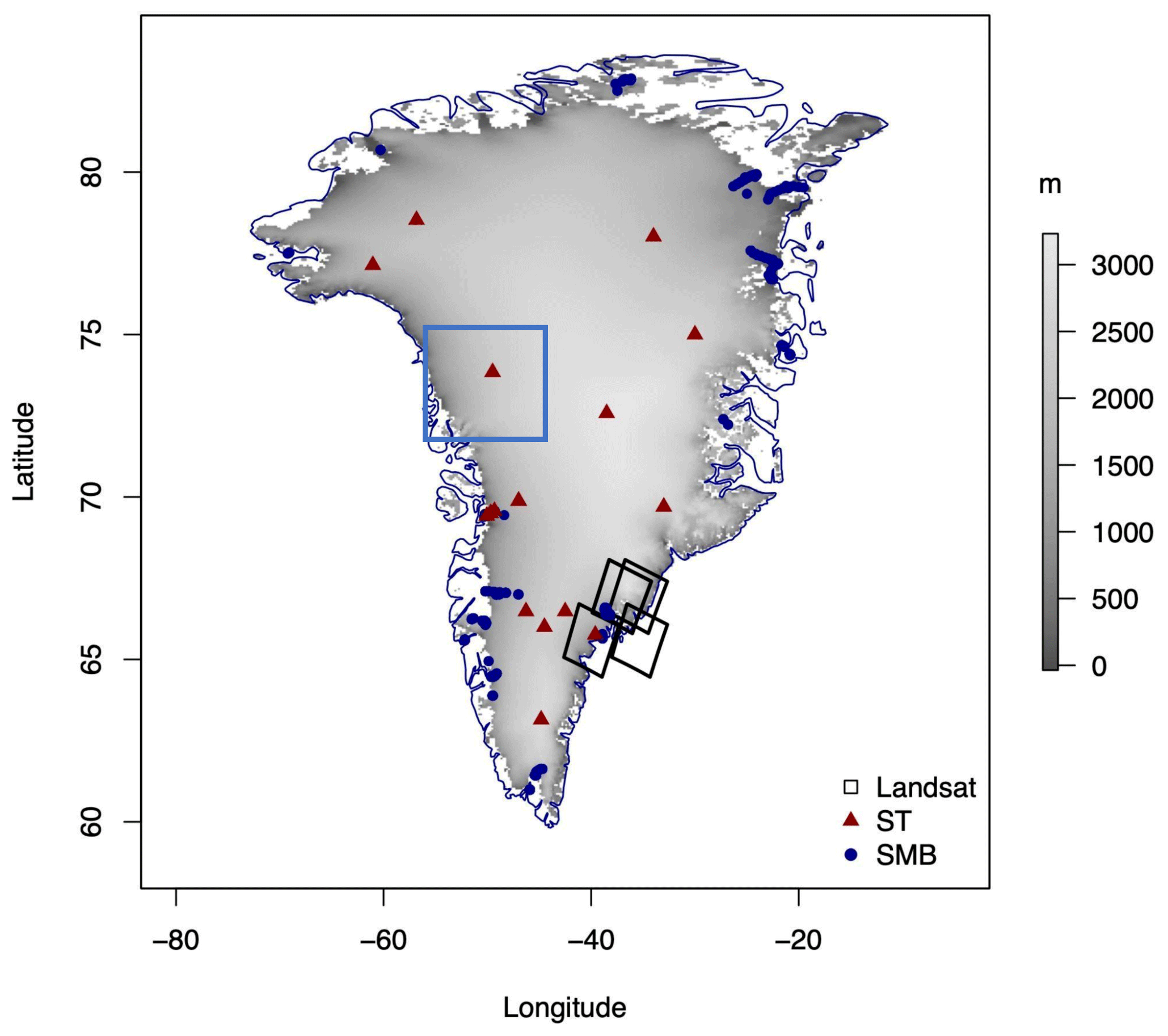
Figure 1 Map of the Greenland Ice Sheet. The digital elevation model (DEM) at 100 m resolution is represented in greyscale, the GC-Net air temperature locations are plotted as red triangles, and the PROMICE surface mass balance measurement locations are shown as blue dots. The two rectangles indicate the Jakobshavn (blue) and Helheim (black) regions.

2.2 Digital elevation model

For the digital elevation model (DEM), we adopt the ArcticDEM data product (Porter et al., 2018; Fig. 1). ArcticDEM is a National Geospatial-Intelligence Agency (NGA) and National Science Foundation (NSF) public–private initiative to produce high-quality DEM of the Arctic applying stereo auto-correlation techniques to high-resolution optical satellite images and adopting the SETSM open-source photogrammetric software (Noh and Howat, 2015). Further information about the dataset can be found at https://www.pgc.umn.edu/data/arcticdem/ (last access: 15 November 2023). Specifically, we use a DEM provided at the spatial resolution of 100 m. The data are projected to the National Snow and Ice Data Center (NSIDC) Sea Ice Polar Stereographic North and referenced to WGS84 datum. The overall dataset is composed of 403 920 000 cells and is distributed as a GeoTIFF with a total size of approximately 1.6 Gb.

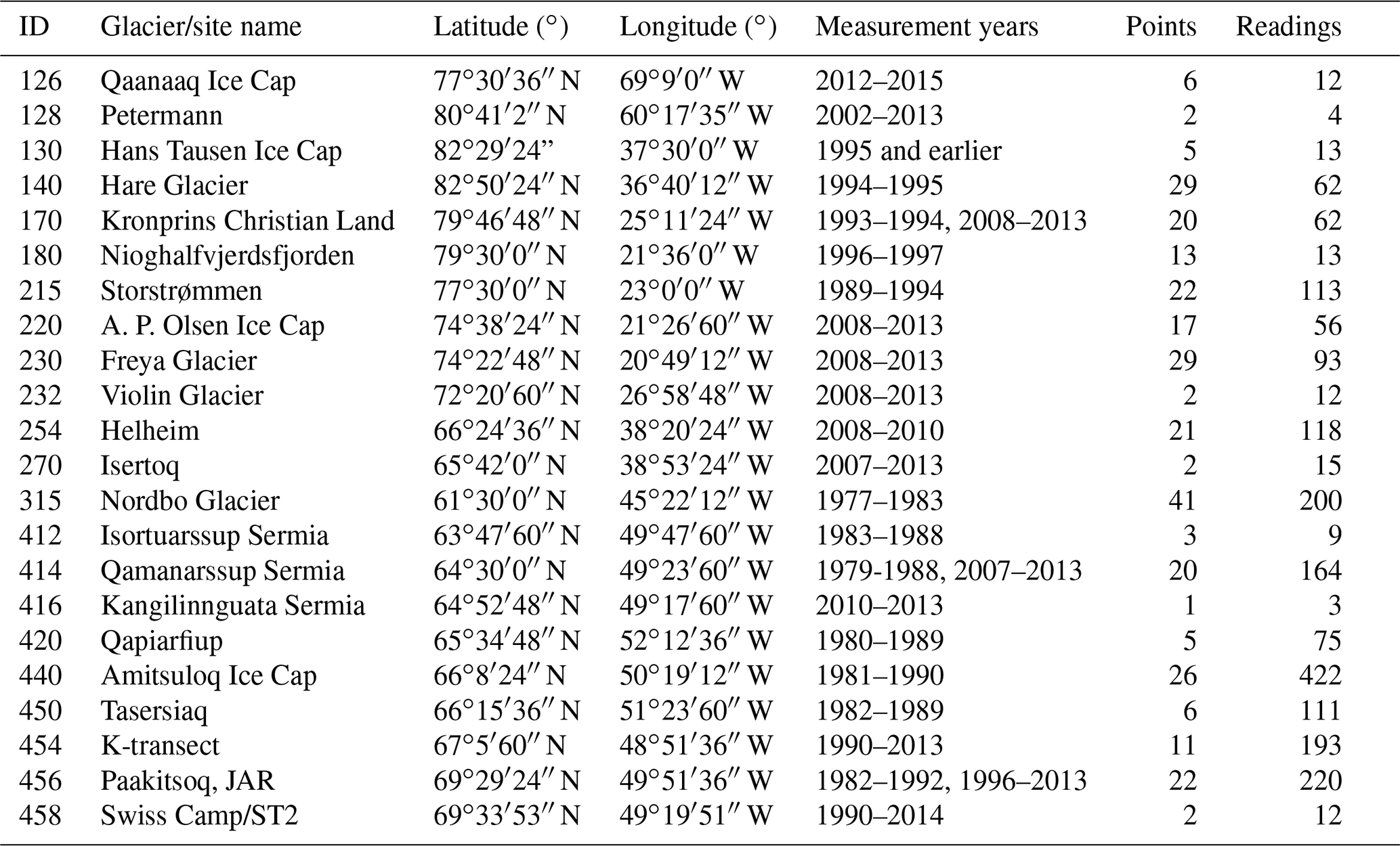
Table 1 PROMICE surface mass balance measurements information for the selected glaciers and measurement sites.

2.3 PROMICE surface mass balance measurements

The main objective of this work is to obtain a high-resolution SMB dataset from the downscaling of the MAR model suitable for local (i.e., glacier scale) studies. Consequently, we carried out a validation of our results by comparing the original SMB outputs from MAR at a spatial resolution of 6 km and the downscaled outputs at 100 m with in situ SMB measurements. For this purpose, we used the dataset collected by Machguth et al. (2016), containing 2955 SMB measurements from 46 sites, reported in Fig. 1 as blue dots and available on GEUS Dataverse portal (Machguth, 2022). This comprehensive dataset spans from 1892 to 2015. From the 123 years, we focused our attention to the period 1980–2015 when the largest portion of the dataset is temporally located and the MAR outputs are available. From the 2955 measurements we obtained 1982 suitable SMB measurements to be used for validation. The SMB measurements are carried out by computing the difference in stake readings between two dates. The observations are identified by the measuring site (i.e., the area or location, containing at least one measuring point), measuring point (i.e., specific stakes, associated with multiple readings), and the actual readings (i.e., the SMB measurement). In Table 1 we report the number of readings for each measuring site considered, together with its coordinates (WGS 84) and time period when the measurements were collected. Measurement periods are various, covering specific seasons (summer or winter SMB) or an entire year (annual SMB). In some cases, short-term (at least 1 month) and multi-year measurements are also present. We reconstructed the SMB in correspondence with the measurement location as an algebraic sum of the daily simulated SMB between the start and end dates of the measurement. As a metric to assess the performance of the downscaled product, we compute the root-mean-square error (RMSE) and the least-square linear regression parameters (slope and intercept) between model outputs (SMB original and downscaled) and measurements (in that order).

2.4 GC-Net air temperature

To test the results of the applied downscaling procedure at local scale we also compare the values of near-surface air temperature obtained from MAR with in situ measurements. We use data from the Greenland Climate Network (GC-Net; Steffen et al., 1996), a set of Automatic Weather Stations (AWSs) located all around the GrIS that continuously measure air temperature, wind speed, wind direction, humidity, pressure, and other parameters. Since direct measurements of surface temperature are not available as continuous records at multiple sites around Greenland, we use the air temperature records measured at 3 m a.g.l. Specifically, we consider 17 selected stations, reported in Fig. 1 as red triangles. Specific locations and elevations for each station are also reported in Table 2 in Sect. 3. The AWS thermometers collect air temperature measurements at sub-daily temporal scale, while MAR outputs are provided at daily temporal resolution. Consequently, we compute daily average air temperatures for the comparison with the modeled and downscaled near-surface temperatures (TT variable).

2.5 Landsat-8 surface temperature

As in situ measurements are only available at point scale, it is not possible to assess the potential improvement of the downscaling approach on spatially distributed fields. In the absence of spatially distributed, high spatial resolution SMB outputs, we use surface temperature fields from seven different Landsat-8 (Collection 2 Landsat 8-9 OLI, 2023) scenes covering the Jakobshavn and the Helheim glaciers, acquired on 5 and 30 June 2015 (two images), 9 July 2015 (two images), and 16 and 18 July 2015. The Landsat-8 surface temperature product has been available at 30 m spatial resolution since April 2013 and is generated from Landsat Collection 2 Level-1 thermal infrared bands and other parameters obtained from satellite observations and reanalysis data. The images were downloaded from the USGS Earth Explorer data portal (https://earthexplorer.usgs.gov/, last access: 17 January 2023). We compared the Landsat-8 observations with the original and downscaled MAR outputs of surface temperature (ST variable).

2.6 Methods

2.7 Downscaling methodology

We adopted the approach used by Noël et al. (2016), in which a statistical downscaling method was applied to RACMO to achieve a 1 km horizontal resolution. Here, we use a similar methodology applied to MAR but instead downscale the product to 100 m horizontal resolution. The method exploits the potential dependency of the modeled variables (e.g., surface temperature, runoff) with elevation. In order to overcome the large number of cells and reduce the computational time, we parallelized the procedure through a combination of geospatial tools (in the software R) so that our approach can also be used for near-real-time generation of downscaled maps over a specific region of the GrIS.

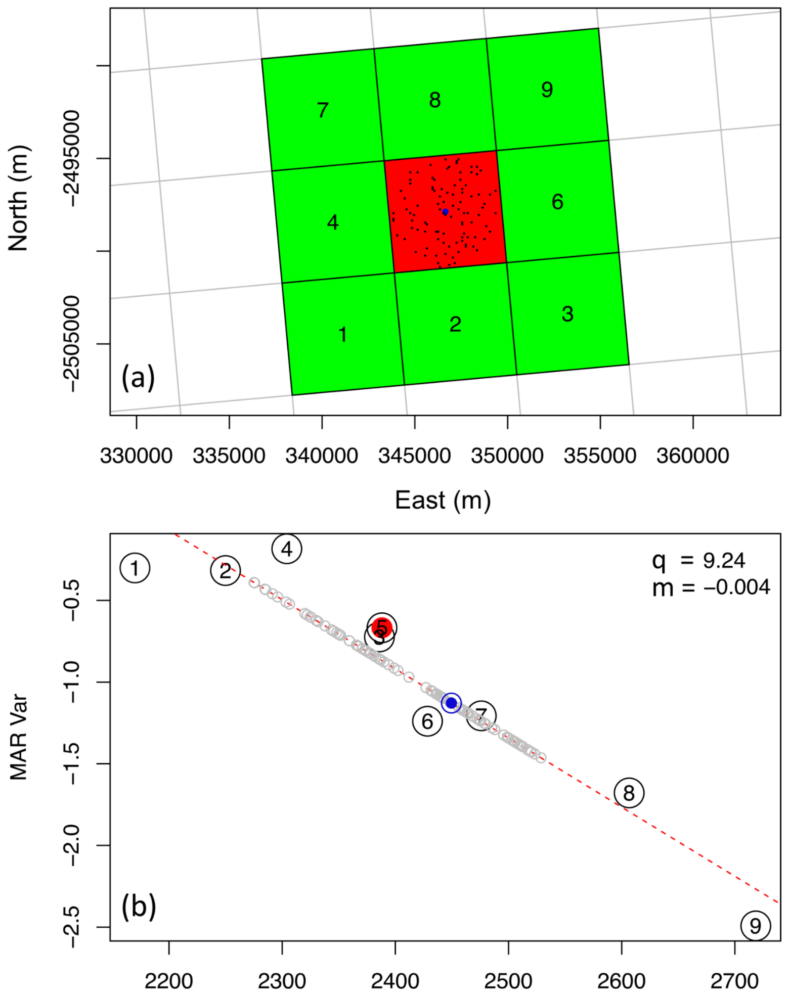
Figure 2 Elevation downscaling procedure example for a generic variable. (a) The considered MAR pixel (red) and the surrounding pixels (green) adopted for the local linear regression are represented. The blue dot represents 100 m pixel location centered within the considered MAR pixel. (b) The variable value of each considered pixel is reported as a numbered circle. The dashed red line represents the linear regression computed for such pixels, the blue circle represents the downscaled variable for the blue pixel in (a), and the grey circles represent the downscaled variable for a group of 100 m pixels randomly picked within the considered MAR pixel, the locations of which are represented as black dots in (a).

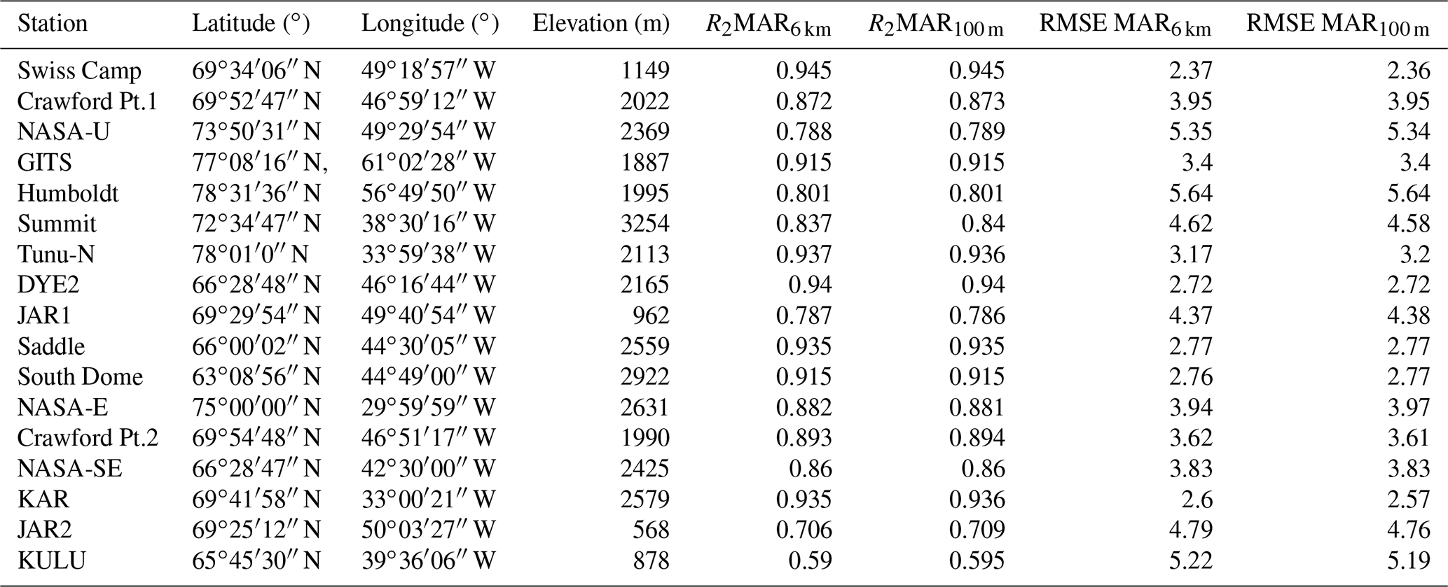
Table 2 Root-mean-square error and R² computed comparing MAR_6 km and MAR_100 m with air temperature measurements from the considered GC-Net stations. Longitude, latitude, and elevation of the station are also reported.

The first step involves the calculation of the local dependency of the MAR outputs with respect to the elevation. For this step we refer to the methodology proposed by Noël et al. (2016). Accordingly, we compute the local linear regression (least squares) between the specific variable and the elevation (obtained from the MAR DEM) obtaining the values of slope (m_6 km) and intercept (q_6 km). The linear regression is carried out for each pixel of the MAR 6 km resolution DEM using the values of the adjacent pixels with a minimum of six points used for the regression. In the case of pixels with fewer than five adjacent pixels (e.g., margins of the ice sheet), we compute m and q for that pixel by interpolation. Such regression is carried out for every day and pixel of the region of interest. Figure 2 provides an example of such a procedure. Parallelizing this procedure for each MAR pixel, we obtain the daily maps of m_6 km and q_6 km for the considered MAR output variable. Differently from Noël et al. (2016), we downscale the SMB output of MAR directly, rather than downscaling the components of the SMB (runoff and sublimation) and then approximating SMB as the sum of its components. We opted for this choice because we found that downscaling SMB directly provides better performance in terms of the downscaling when compared with in situ measurements. Following this, the m_6 km and q_6 km maps are reprojected to the Polar Stereographic coordinate system used by the DEM. The original MAR data are distributed by providing only the coordinates for the center of each grid cell. To create a continuous grid and avoid introducing errors, the coordinates for the four corners of each MAR grid are computed, and they are then transformed into the Polar Stereographic coordinate system. The result is a shapefile that contains a polygon for each MAR grid. Additionally, the new shapefile contains metadata to ease computations, such as a unique MAR grid ID, the Polar Stereographic coordinates for the center of the grid, and the corresponding coordinates in longitude and latitudes for the center of the grid. The next step consists of fragmenting the high-resolution DEM into a series of smaller files, specifically one for each polygon of the reprojected MAR cells generated in the previous steps. There are a total of 55 144 files generated through each step, which is less than the total number of cells in the original MAR output. This discrepancy is due to the fact that the DEM is limited to only areas covered by the ice sheet, and it thus does not cover all the locations of where MAR output is generated. While it might seem counterintuitive that maintaining over 55 000 small files is more efficient than maintaining a single file, the answer lies in the fact that this preprocessing step translates our problem into a parallelization one that can be efficiently solved using multi-core and multi-node infrastructure. Because the DEM is required for downscaling each grid cell, which are computed simultaneously in parallel, each task needs to read only a small file of a few kilobytes, rather than one larger file, and it also avoids file system bottlenecks when multiple processes try accessing the same file. Most file systems do not allow for concurrent access to the same file, and therefore if hundreds of tasks try to read the same file, each task would have to idle in a queue for the file access to become available. This problem is prevented by generating a DEM file for each MAR grid so that input and output transfer rate and file access are both optimized. Furthermore, because the DEM is segmented using the original Polar Stereographic projection, which matches the reprojected MAR grid, no further transformation is required, further speeding up the downscaling process. The final step consists of obtaining the high-resolution maps of slope and intercept (m_100 m and q_100 m) by bilinear interpolation of m_6 km and q_6 km over the high-resolution DEM grid. While this process was not parallelized in the current version, it is possible to speed it up using a parallel solution. Finally, the downscaled variable is obtained by applying the high-resolution linear regression coefficients to the high-resolution DEM as

$$\begin{array}{}\text{(1)}& {\text{VAR}}_{\mathrm{100}\mathrm{m}}=m_{\mathrm{100}\mathrm{m}}{H}_{\mathrm{100}\mathrm{m}}+q_{\mathrm{100}\mathrm{m}},\end{array}$$

where VAR is the generic downscaled variable computed as a linear function of high-resolution elevation of the DEM (H_100 m) through the coefficients previously obtained (m_100 m and q_100 m). Since the origins of the MAR DEM and the high-resolution DEM are different, errors in terms of mass conservation can arise. For example, within a MAR pixel the average elevation of the high-resolution DEM might be higher than the original MAR elevation, possibly leading to the previously mentioned mass conservation error (e.g., the original MAR pixel suggests for a day a lower mass loss than the ensemble of the high-resolution pixels). For this reason, in contrast with Noël et al. (2016), we decided to provide physical constraints (SMB mass conservation within each pixel at the original MAR spatial resolution) to be satisfied as the very final step of the downscaling procedure.

In this research, we apply the downscaling methodology to daily near-surface temperature, surface temperature, and SMB MAR outputs.

2.8 Spatial autocorrelation analysis and variograms

Beside RMSE, slope, and intercept, we also focus on evaluating the potential improvements of the downscaled product with respect to the original coarser-resolution MAR outputs in terms of capability to describe the spatial distribution of the considered variable. To this end, we perform a spatial autocorrelation analysis using variograms. Variogram analysis is generally adopted in geostatistical analyses to evaluate autocorrelation of spatial data (Edward et al., 1989; Webster and Oliver, 2001). Autocorrelation and variogram analysis are geostatistical tools that can be used to quantify spatial variability using metrics such as the spatial correlation length (hereafter simply referred to as correlation length). Though these techniques were mainly designed to support the prediction of values at locations where measurements are not available, they can be used for characterizing processes across the scale spectrum (Herzfeld, 1993). Once process scales are known, the scale ranges over which process relationships (and thus spatial pattern) are consistent must be determined. This can support the identification of spatial scales at which the process interactions change (e.g., scale breaks), as such scales are critical for measurement or model interests (Mark and Aronson, 1984; Vedyushkin, 1994). Geostatistical methods such as spatial covariance, variogram analysis, and spectral analysis (Webster and Oliver, 2001) quantify the spatial pattern of variability of an observed property over a scale range from the minimum sample separation to the distance at which the variable becomes spatially independent. This quantified variability can then be used for spatial estimation based on a finite number of data points. In our case, we fit the experimental variogram with a circular model, as this is the model that provided us with the highest R² when fitting the experimental data. The formal expression of the experimental variogram can be written as follows:

$$\begin{array}{}\text{(2)}& \mathit{\gamma }\left(\mathit{\delta }\right)={\displaystyle \frac{\mathrm{1}}{\mathrm{2}N\left(\mathit{\delta }\right)}}{\sum }_{i,j\in N\left(\mathit{\delta }\right)}(x_i-x_j{)}^{\mathrm{2}},\end{array}$$

where γ is the semi-variance, N(δ) is the number of data pairs (ith and jth) distanced by d, while x_i and x_j are the corresponding variable values. The fitting spherical function is then used to compute the three main parameters characterizing the variogram: the sill, the range, and the nugget effect. The sill is defined as the maximum value at which the fitted curve becomes flat; such a variance value is reached at a certain distance called range, beyond which the data are no longer autocorrelated. The range can be seen as a scale break (where data are no longer correlated). Of course, there can also be several scale breaks before the sill is reached, depending on the drivers controlling the modeled process. The nugget corresponds to γ(0) and it should ideally be 0. The departure from 0 can be interpreted as the result of measurement errors or highly localized variability (Webster and Oliver, 2001). Following Colosio et al. (2021), we focus our attention on the range, the descriptor of the correlation length, comparing the range values computed for the original MAR temperature outputs, the downscaled temperature, and the surface temperature observed by Landsat-8.

To further investigate and quantify possible improvements in terms of spatial description of the variable of interest by the downscaled product, we also compute the so-called structural similarity index measure (SSIM). Such an index has been introduced by Wang et al. (2004) to provide a similarity measure between two images. This index can objectively quantify a qualitative aspect such as the similarity between two images. Considering a pair of images (X,Y) to be compared, the values assumed by the SSIM are bounded by a unique maximum (SSIM(X,Y) = 1) in case X = Y, otherwise SSIM(X,Y) < 1. We compute such a similarity index for both original and downscaled MAR ST outputs, considering as reference the Landsat-8 surface temperature image.

3 Results and discussion

3.1 Surface and near-surface temperature

We first tested the downscaling algorithm with the MAR near-surface temperature outputs. We compared the results obtained with air temperature measurements from 17 AWS of the GC-Net. We performed the comparison by computing RMSE and R² between the modeled (original and downscaled) and the observed variable. The results obtained for the original MAR and the downscaled temperatures are reported in Table 2. Both R² and RMSE obtained for the downscaled temperatures do not exhibit significant improvements or worsening with respect to the original coarser-resolution output. The difference between the 6 km and 100 m resolution is on the order of 10⁻³ for R² and 10^−2 ∘C for RMSE, with improvements in some stations (Swiss Camp, Crawford Pt. 1, NASA-U, Summit, Crawford Pt. 2, KAR, JAR2, and KULU) and worsening in others (Tunu-N, JAR1, South Dome, and NASA-E). However, such small differences appear to be randomly distributed in space, without any clear correlation with elevation, latitude, or longitude. Such results demonstrate that the applied downscaling methodology does not introduce errors in the case of the TT variable at point scale.

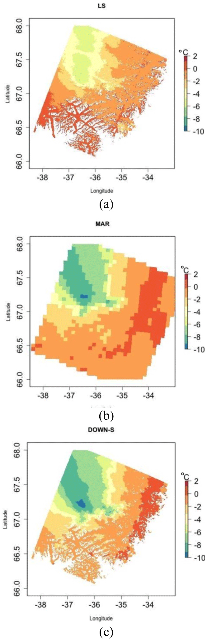
Figure 3 Maps of temperature from (a) Landsat-8, (b) MAR_6 kmv2, and (c) MAR_100 m over the area covered by the Landsat-8 selected image on 30 June 2015.

To evaluate the results over a wider area, we considered two Landsat-8 surface temperature images collected over two different areas of the ice sheet. The two selected areas are located on the eastern and western coasts of Greenland and show a variable topography. In Fig. 3 we report the surface temperature image from Landsat-8 (Fig. 3a), the original ST output at 6 km spatial resolution (Fig. 3b), and the downscaled ST at 100 m resolution (Fig. 3c) for one of the selected Landsat-8 scenes. In Fig. 4 we report the histograms of the difference between Landsat-8 surface temperature and the original ST (Fig. 4a) and the downscaled one (Fig. 4b) for the same image. The results show no change in terms of mean difference (μ), with an average difference of 2.7 ^∘C in both cases, similar to the AWS comparison. In addition, the standard deviation (σ) remains unvaried at 2.6 ^∘C. Similar results have been obtained for all the compared Landsat-8 images, with mean differences ranging between −0.59 and 3.44 ^∘C for the downscaled product (2.09 ^∘C on average) and between −0.62 and 3.43 ^∘C for the original MAR data (2.07 ^∘C on average). The similarity in mean differences is not surprising considering the physical constraints imposed for the ST to maintain the average ST constant for each MAR pixel as the final step of the downscaling procedure. These results indicate that in case of ST the downscaling algorithm does not introduce significant improvements or errors in terms of overall difference with observed temperature (expressed as RMSE for the AWS case and spatial average difference for the Landsat-8 image).

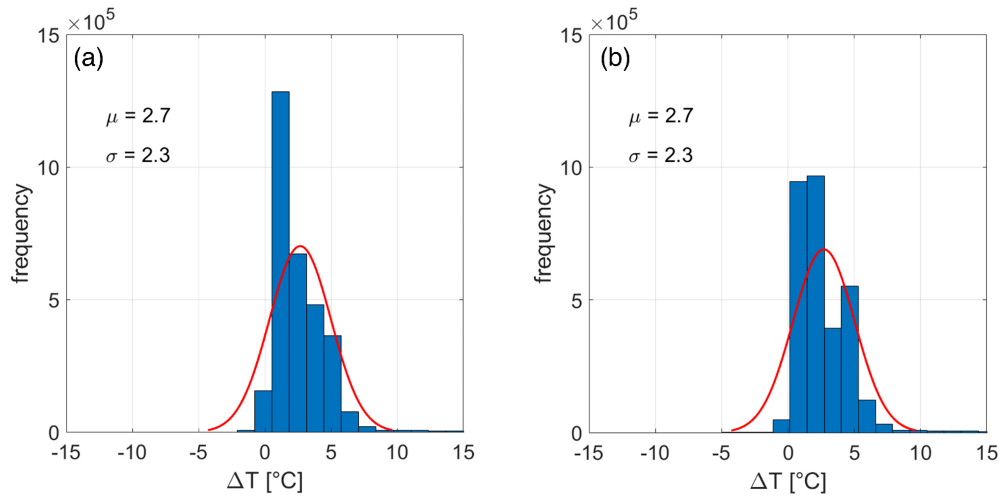
Figure 4 Histograms of the difference (a) between the 6 km MAR temperature and Landsat-8 temperature and (b) between 100 m MAR temperature and Landsat-8 temperature.

Considering such results in terms of difference at point scale and spatially averaged difference, we evaluated possible improvements in terms of spatial information content and spatial description obtained in the downscaled product. In Fig. 5 we report the results of the variogram analysis performed for two sub-regions of interest within the same Landsat-8 image shown in Fig. 3. The two areas have been selected because of the strong differences in topography and elevation gradients. Concerning the results obtained over the topographically more complex area, we observe that the scale break of the downscaled temperature (blue line) is 13.5 km, better capturing the one from Landsat-8 data (11.5 km, red line) with respect to the original MAR outputs (24.1 km, black line, Fig. 5). On the other hand, the same analysis performed over an area in a more interior region of the ice sheet, where downscaling might lead to less improvement in view of the reduced topography, does not present improvements in terms of spatial autocorrelation (Fig. 5b), and all three datasets do not reach the variogram plateau within the considered distance. In order to extend the comparison to another area of the ice sheet, we performed the same variogram-based analysis for another Landsat-8 scene in the surroundings of Jakobshavn glacier collected on 11 June (Fig. 6a). The map also shows the two regions of interest (ROIs) selected for the analysis. We selected ROI₁ as this area is characterized by a large topographic gradient within a relatively small distance and to understand the potential improvement of the downscaling procedure over regions that are outside the main ice sheet (e.g., smaller glaciers). On the other hand, ROI₂ contains both strong and mild elevation gradients (e.g., nunataks and ice sheet elevation gently increasing as moving towards the interior). In the case of ROI₁ (Fig. 6b), the variogram analysis indicates that the scale break distance for Landsat-8 when considering only the pixels where the DEM is available is 7.5 km. This value becomes 14.6 km for the high-resolution map of ST and 24.7 km in the case of the original MAR outputs, suggesting that the downscaled product is able to perform better than the original one in terms of spatial-scale similarity with respect to the Landsat-8 data. The mean difference between Landsat-8 and the downscaled (original MAR) surface temperature, considering only the pixels where the DEM is available, is 1.69 ^∘C (1.7 ^∘C) with a standard deviation of 2.02 ^∘C (2.14 ^∘C), with differences of the same order of magnitude obtained in the previous analysis for the other Landsat-8 image. When considering all pixels within the ROI (e.g., also where no DEM is available), the mean difference between Landsat-8 and downscaled (original) MAR surface temperature becomes 1.89 ^∘C (2.12 ^∘C) with a standard deviation of 2.15 ^∘C (2.23 ^∘C). In this case, the scale breaks for the original and the downscaled MAR versions are similar, i.e., ∼25 km (∼16 km in the case of Landsat-8). We point out that the scale breaks are sensitive to the different physical processes driving the spatial properties. The ROI₂ contains both strong and mild elevation gradients given the presence of nunataks and the slow ice sheet increasing elevation after the ice cliff begins. The area mostly covers the portion containing the ice sheet (right of the image) in the DEM, which is however absent in the case of the left portion of the ROI, which contains fjords and the ocean. The scale breaks for the Landsat-8 and downscaled and original MAR cases for the portion of the ROI₂ where the DEM is available are close to each other, on the order of ∼25 km. We observe an improvement in the SSIM in the case of the downscaled data by 30 % (from 0.33 in the case of the original MAR resolution to 0.43 in the case of downscaled MAR). Unexpectedly, despite the mean and standard deviation of the distribution of the differences between the Landsat-8 data and the simulated quantities remaining similar, we notice a reduction in both the mean (from 0.86 ^∘C for original MAR to 0.83 ^∘C for the downscaled product) and the standard deviation (from 0.71 ^∘C for original MAR to 0.63 ^∘C for the downscaled product) when downscaling the MAR output. We further note that when considering all pixels (including those with no DEM), the SSIM of the two products improves from 0.11 (original) and 0.14 (downscaled) and that the scale break of the original MAR products is larger (∼63 km) than the one of the Landsat-8 data (∼21 km). In synthesis, the downscaling does not introduce any considerable bias on the original value, preserves the total integrated quantity of energy within each area, and improves the spatial performance of the MAR outputs by generating a product that has a spatial structure that is closer to the one of the observed remote sensing dataset.

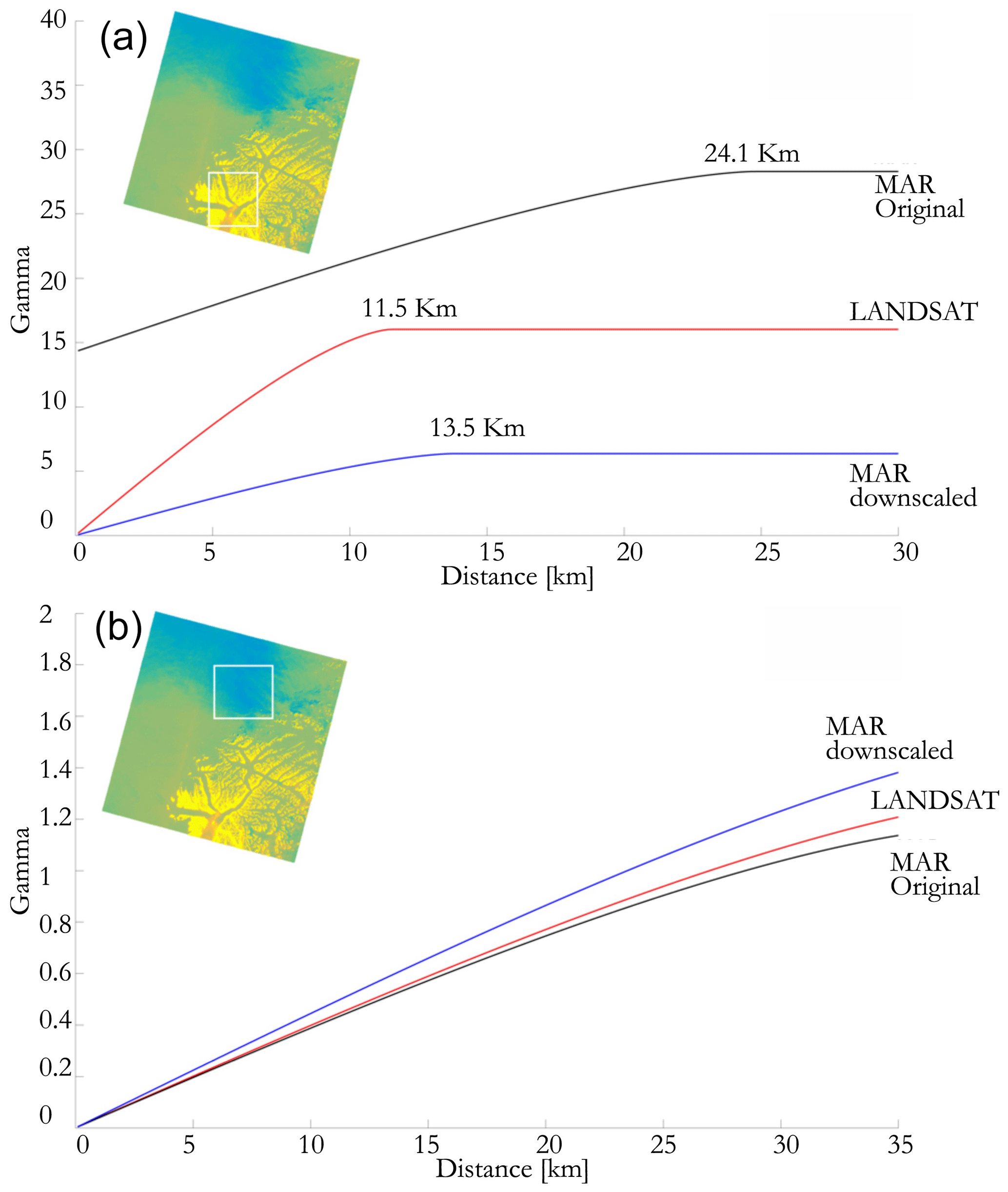
Figure 5 Modeled semi variograms for the Landsat-8, MAR_6 km and MAR_100 m computed over two regions of interest reported in the inset.

3.2 Surface mass balance

After applying the downscaling algorithm to surface temperature, we applied it to MAR SMB outputs of SMB and assessed the results obtained with in situ measurements from the dataset collected by Machguth et al. (2016). As mentioned, we compared 1982 SMB measurements carried out between 1980 and 2015 and localized in the ablation area of the GrIS (Table 1). Figure 7 shows the scatterplots of the comparison of modeled SMB from the original MAR (Fig. 7a) and the downscaled product (Fig. 7b) with in situ measured SMB. Our results show that the downscaled product better estimates the measured SMB, exhibiting an increased R² from an already relatively high value of 0.868 for the original MAR to 0.935 for the downscaled product. As a comparison, Noël et al. (2016) obtained an increase in R² from the downscaling of SMB outputs of the RACMO regional climate model from 0.47 in the case of the original 11 km spatial resolution outputs to 0.78 in the case of the downscaled SMB (1 km resolution). As explained in Fettweis et al. (2020), the SMB was extrapolated (interpolated plus corrected) to the common 1 km grid by applying an elevation gradient as has been done in this study. One of the key issues raised by the first SMB model intercomparison performed by Vernon et al. (2013) was the high dependency of modeled integrated SMB values on the ice sheet mask used. To mitigate this problem, we interpolate all model outputs to the same 1 km grid used in the Ice Sheet Model Intercomparison Project for CMIP6 (ISMIP6). This resolution is chosen because the highest-resolution model outputs (e.g., RACMO2.3p2) are available at 1 km and choosing a coarser resolution could compromise their quality. A common grid also allows a comparison on two common ice sheet masks: the contiguous Greenland Ice Sheet, which is common to all the models, and the Greenland Ice Sheet plus peripheral ice caps and mountain glaciers, common to all the models except the two positive degree day (PDD) models. Unless otherwise indicated, the SMB components have been interpolated to 1 km using a simple linear interpolation metric of the four nearest inverse-distance-weighted model grid cells. Moreover, as done in Le Clec'h et al. (2019), the interpolated 1 km SMB and runoff fields have been corrected for elevation differences between the model native topography and the GIMP 250 m topography (upscaled to 1 km here), using time- and space-varying SMB–elevation gradients, similar to Franco et al. (2012) and Noël et al. (2016). No correction was applied to precipitation after interpolation to 1 km. We point out that in our case the starting value of R² for the original MAR product already exceeds the value obtained in the case of the downscaled RACMO outputs.

The values of slope and intercept of the best-fitting line improve as well when considering the downscaled product. The value of the slope shifts from 0.865 for the original MAR to 1.015 for the downscaled product; similarly, the intercept increases from the value −235 mm w.e. yr⁻¹ of the coarse-resolution outputs to −57 mm w.e. yr⁻¹ of the downscaled SMB, closer to its optimal value (i.e., null intercept). As a comparison, the downscaling algorithm of Noël et al. (2016) applied to RACMO improved the estimate of SMB in terms of slope from 0.72 to 1.03, with a slight increase in the intercept (from 70 to 100 mm w.e. yr⁻¹). The RMSE between modeled and measured SMB also decreases in the case of the downscaled product from 669 mm w.e. yr⁻¹ for the 6 km outputs to 511 mm w.e. yr⁻¹ for the 100 m case, significantly improving the estimate of SMB at local scale. Noël et al. (2016) obtained a reduction in the RMSE passing from a value of 1200 mm w.e. yr⁻¹ for the 11 km RACMO outputs to a value of 740 mm w.e. yr⁻¹ for the 1 km case. Fettweis et al. (2020) compared MAR and RACMO, among 13 models of four types (positive degree day models, energy balance models, regional climate models, and general circulation models), and SMB estimates with the same PROMICE in situ measurements within the GrIS SMB model intercomparison project (GrSMBMIP). They considered only the measurements collected between 1980 and 2012 and with measurement periods longer than 3 months. They also excluded the records located outside the 1 km ice mask they used for the intercomparison of the models, for a total of 1438 SMB measurements. The model versions in this case are MARv3.9.6, an older version than the one we adopted and at the spatial resolution of 15 km, and RACMO2.3p2 (Noël et al., 2019), a new version of the one adopted in Noël et al. (2016) and with a spatial resolution of 5.5 km. From the comparison, they obtained a RMSE of 480 mm w.e. yr⁻¹ for MAR and 630 mm w.e. yr⁻¹ for RACMO. In both cases, the RMSE is lower than the one obtained in this work for MAR (both original and downscaled) and by Noël et al. (2016) for RACMO. The difference can be related to the differences in spatial resolution and model versions and most probably to the sub-sampling of the SMB measurements discarding short-term records (i.e., measurement period lower than 3 months), suggesting that the bias might be dissipated for longer observation periods.

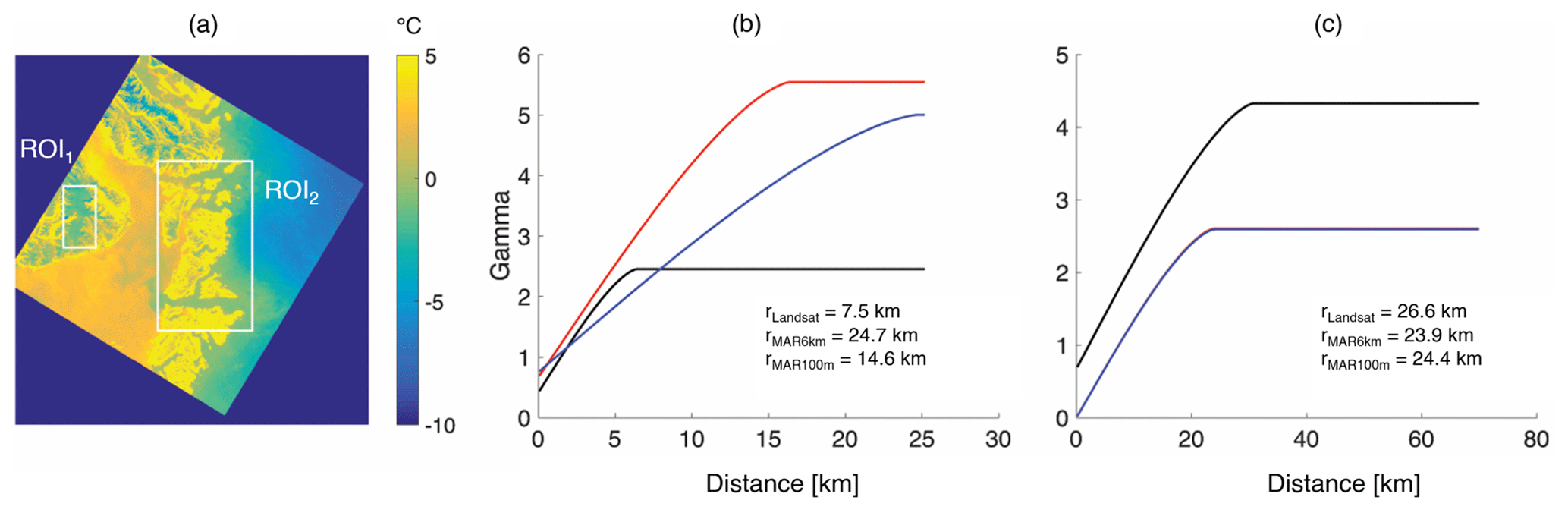
Figure 6 (a) Landsat-8 temperature captured on 11 June 2015 over areas around the Jakobshavn Glacier and (b, c) modeled semi-variograms for the Landsat-8 (black), MAR_6 km (blue), and MAR_100 m (red) computed over (b) the first region of interest (ROI₁) and (b) the second region of interest (ROI₂).

To further investigate our results, we compute the variation in RMSE between the 6 km spatial resolution MAR outputs and the downscaled product for different elevation classes, longitude and latitude ranges, and each specific glacier or location (i.e., for each station ID; see Table 1) of the PROMICE in situ SMB dataset. The RMSE difference is computed as ΔRMSE = RMSE_100 km−RMSE_6 km (i.e., improvements are characterized by negative values of ΔRMSE) and the results obtained are reported in Fig. 8 grouped by location (Fig. 8a), elevation (Fig. 8b), latitude (Fig. 8c), and longitude (Fig. 8d). The results exhibit improvements in the estimate of SMB at all the altitudes besides the 100–200, 200–300, and 1300–1400 m a.s.l. elevation classes, with the best performance obtained at 700–800 and 800–900 m a.s.l. elevation classes. The results grouped by latitudinal bands show the highest improvements in southern Greenland; a decrease in performance has been recorded in the latitudinal band 67.5–70^∘ N, where the only Paakitsoq JAR (ΔRMSE = 181 mm w.e. yr⁻¹, worst result obtained) and Swiss Camp/ST2 (ΔRMSE = −127 mm w.e. yr⁻¹) measurement sites are located, and the improvement obtained in case of Swiss Camp is strongly counterbalanced by the reduced performances in Paakitsoq JAR. However, the longitudinal classes do not present any decrease in performance, indicating that the worsening in the spotted critical stations is counterbalanced by the improvements measured in the others. We obtained a decrease in performance in 6 out of 22 considered cases, with the worst result obtained for the already presented Paakitsoq JAR case. In the five other cases (i.e., Hans Tausen Ice Cap, Nioghalfvjerdsfjorden, Isortoq, Nordbo Glacier, and K-transect) we recorded an average ΔRMSE of 26 mm w.e. yr⁻¹ (ranging from 6 to 80 mm w.e. yr⁻¹). On the other hand, we obtained an improvement in 16 out of 22 measurement sites, with the best performances in the case of A. P. Olsen Ice Cap (ΔRMSE = −611 mm w.e. yr⁻¹). In the other 15 cases (i.e., Qaanaaq Ice Cap, Petermann, Hare Glacier, Kronprins Christian Land, Storstrømmen, Freya Glacier, Violin Glacier, Helheim, Isortuarssup Sermia, Qamanarssup Sermia, Kangilinnguata Sermia, Qapiarfiup, Amitsuloq Ice Cap, Tasersiaq, and Swiss Camp/ST2) we found an average decrease in RMSE of 183 mm w.e. yr⁻¹ (ranging between 59 mm w.e. yr⁻¹ and 371 mm w.e. yr⁻¹). Even if such reduction in performance in terms of SMB estimate accounts for 27 % of the considered stations, it does not compromise the overall improvement, being smaller in terms of average, minimum, and maximum absolute values of ΔRMSE than the results obtained for the stations where improvement occurred.

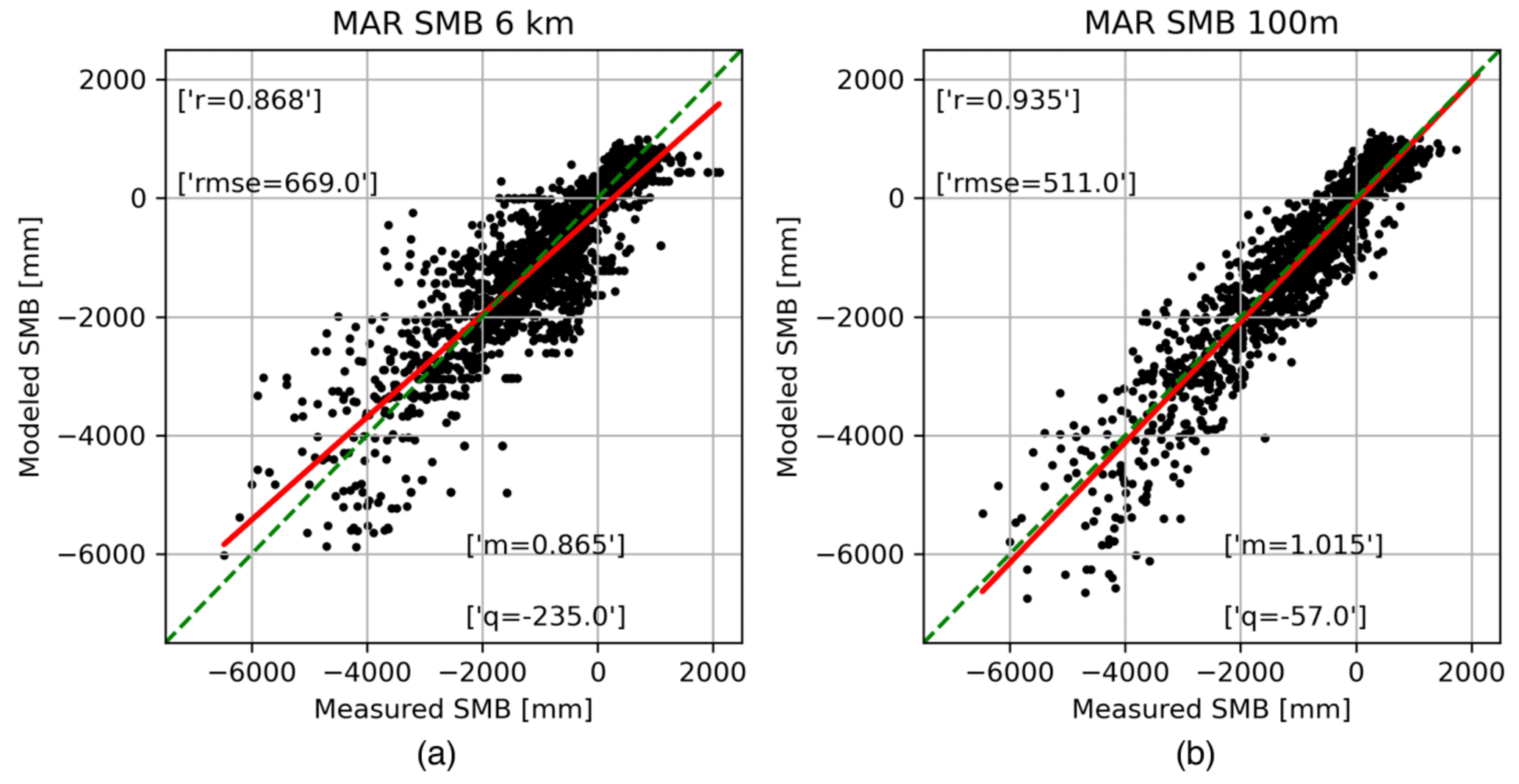
Figure 7 Comparison between measured and modeled surface mass balance from (a) the original 6 km MAR and (b) the downscaled 100 m MAR.

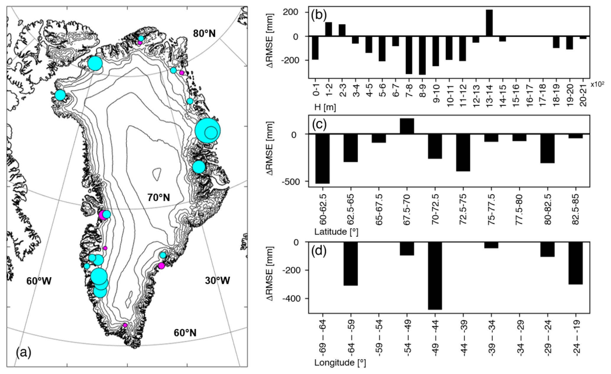
Figure 8 Difference between original and downscaled MAR modeled surface mass balance RMSE with respect to the measured surface mass balance data (RMSE_100 m−RMSE_6 km) by (a) glacier, (b) elevation, (c) latitude, and (d) longitude. In the bubble chart map the contour lines are plotted every 500 m (original MAR_6 km DEM), and positive values (worsening) of ΔRMSE are reported in magenta, while negative values (improvement) are reported in cyan.

4 Conclusions and future work

We applied a statistical downscaling technique to increase the horizontal spatial resolution of the outputs of the MAR regional climate model from 6 km to 100 m for the surface temperature and SMB quantities. The approach builds on the dependency of such quantities on elevation, as originally proposed in Noël et al. (2016). Here, however, the technique was applied to the output of a different climate model (RACMO), and the spatial resolution of the downscaled product was 1 km rather than 100 m. Moreover, differently from Noël et al. (2016), we imposed mass conservation so that the overall mass obtained for each pixel at high resolution nested within a coarse-resolution pixel is preserved. To address the computational issues associated with the relatively high spatial resolution, we developed a geospatial, parallelized framework that allows us to perform the downscaling over the whole ice sheet in an efficient way.

We first tested our approach by applying it to surface temperature data and assessing the outputs using both in situ and satellite data. Our results showed no significant improvement or deterioration of the downscaled product with respect to the original MAR outputs. This confirms that our approach was not introducing any bias and was properly implemented. However, we found improvement in the downscaled surface temperature when analyzing the skills of the downscaled product to capture the spatial scales (e.g., scale breaks) of the observed surface temperature fields. The results obtained in the case of the SMB show a considerable improvement in the case of the downscaled product with respect to the original coarse output. In the case of the downscaled MAR product, the R² value increases from 0.868 for the original MAR to 0.935 for the SMB product, with the value of the slope and intercept shifting from 0.865 for the original MAR to 1.015 for the downscaled product in the case of the intercept and from the value −235 mm w.e. yr⁻¹ of the coarse-resolution outputs to −57 mm w.e. yr⁻¹ in the case of the slope. As a reference, Noël et al. (2016) obtained an increase in R² from the downscaling of SMB outputs of the RACMO regional climate model from 0.47 in the case of the original 11 km spatial resolution outputs to 0.78 in case of the downscaled SMB (1 km resolution) and a shift in the slope and intercept from 0.72 to 1.03 (slope) and from 70 to 100 mm w.e. yr⁻¹ (intercept). An analysis of the performance of the downscaled product for different elevation classes, longitude and latitude ranges, and each specific glacier or location where SMB in situ data are available shows that the downscaled product does not perform as expected for 27 % of the stations. However, we point out that the deterioration of the performance over those stations (expressed in terms of changes on the average error ΔRMSE) is much smaller than the improvement obtained in the remaining cases.

The next step is to implement a similar approach for downscaling MAR outputs over both the Greenland and Antarctic ice sheets using machine learning (ML)-based approaches. Indeed, the approach proposed here cannot be easily extended to Antarctica, where surface melting does not exhibit a strong dependency on elevation, as most of it occurs over ice shelves, at sea level, and where only small elevation gradients exist. Moreover, improvements to the downscaling of the SMB can be obtained by either considering complementary inputs that can improve estimates of losses (e.g., remotely sensed albedo) or of mass gains (e.g., accumulation). ML tools can help in this regard. ML tools have indeed been used for improving predictions beyond that of state-of-the-art physical models or for improving parameterization in models. In particular, conditional generative adversarial networks (C-GANs or simply GANs in the following) can be successfully applied to the problems discussed above (Goodfellow et al., 2014). GANs is a class of ML tools in which two neural networks compete with each other in a minimum–maximum optimization problem. The first network, called the generator, aims to generate new data samples that are indistinguishable from the training data (e.g., high-resolution melting maps obtained from the remote sensing observations) by the other network, called the discriminator. In our case, the GAN aims to generate high-resolution melting maps that are indistinguishable by the second network from high-resolution remote sensing observations or numerical model outputs. We have already started to build the architecture for this framework, are in the phase of collecting the necessary datasets, and are building the proper data framework to perform such work.