the Creative Commons Attribution 4.0 License.
the Creative Commons Attribution 4.0 License.
 | 22 Nov 2023
Combined GNSS reflectometry–refractometry for automated and continuous in situ surface mass balance estimation on an Antarctic ice shelf
Ladina Steiner
Holger Schmithüsen
Jens Wickert
Olaf Eisen
Reliable in situ surface mass balance (SMB) estimates in polar regions are scarce due to limited spatial and temporal data availability. This study aims at deriving automated and continuous specific SMB time series for fast-moving parts of ice sheets and shelves (flow velocity > 10 m a−1) by developing a combined global navigation satellite system (GNSS) reflectometry and refractometry (GNSS-RR) method. In situ snow density, snow water equivalent (SWE), and snow deposition or erosion are estimated simultaneously as an average over an area of several square meters and independently on weather conditions. The combined GNSS-RR method is validated and investigated regarding its applicability to a moving, high-latitude ice shelf. A combined GNSS-RR system was therefore installed in November 2021 on the Ekström ice shelf (flow velocity ≈ 150 m a−1) in Dronning Maud Land, Antarctica. The reflected and refracted GNSS observations from the site are post-processed to obtain snow accumulation (deposition and erosion), SWE, and snow density estimates with a 15 min temporal resolution. The results of the first 16 months of data show a high level of agreement with manual and automated reference observations from the same site. Snow accumulation, SWE, and density are derived with uncertainties of around 9 cm, 40 kg m−2 a−1, and 72 kg m−3, respectively.
This pilot study forms the basis for extending observational networks with GNSS-RR capabilities, particularly in polar regions. Regional climate models, local snow modeling, and extensive remote sensing data products will profit from calibration and validation based on such in situ time series, especially if many such sensors will be deployed over larger regional scales.
- Article
(3261 KB) - Full-text XML
- BibTeX
- EndNote


The potential contribution of the Antarctic ice sheet to the rise in sea level is significant as it contains approximately 80 % of the world's freshwater (Vaughan et al., 2013; King et al., 2012). Ocean warming, variation in atmospheric circulation patterns, and enhanced atmospheric moisture lead to increased snowfall, which dominates the observed positive trend in the East Antarctic ice sheet mass balance (Shepherd et al., 2012). Currently, the mass gain of the East Antarctic ice sheet potentially exceeds the increased mass loss of the West Antarctic ice sheet (e.g., Medley and Thomas, 2019), thus mitigating the rise in the global sea level. Davison et al. (2023) “emphasize the important impact of extreme snowfall variability on the short-term sea level contribution from West Antarctica”.
However, the surface mass balance (SMB) estimates remain a significant uncertainty factor in ice sheet mass balance computation and projections due to the scarce spatial and temporal availability of in situ data (van den Broeke et al., 2017, 2009). Rising global temperatures are projected to lead to increased solid ice discharge, surface melt, and SMB, necessitating continuous time series of in situ snow density, snow water equivalent (SWE), and snow deposition or erosion for correct SMB estimates and, thus, sea level rise predictions (e.g., Gardner et al., 2013; Hanna et al., 2008). Future mass balances are therefore provided by prognosis for various scenarios, using regional climate models, which are affected by uncertainties from applied density assumptions (e.g., van Wessem et al., 2018). Validation and calibration are based on very limited annual accumulation estimates from radio-echo sounding, firn and ice cores, snow pits, or unevenly distributed weather stations with limited information about snow or firn conditions.
Extensive observations of SMB are a challenging task due to the heterogeneity of snow distribution caused by inhomogeneous snow deposition and ablation. Large-scale Antarctic ice sheet changes and snow observations can be derived from spaceborne radar interferometry (e.g., Rignot et al., 2011). The observations of gravity (e.g., Soerensen and Forsberg, 2010; Velicogna and Wahr, 2005) provide direct mass changes. Repeat laser altimetry, such as those from airplanes or satellites, can quantify snow or firn surface-elevation changes (e.g., Markus et al., 2017; Helm et al., 2014). These remote sensing techniques cannot provide direct estimates of SMB, snow or firn density, and SWE; thus they necessitate accurate and reliable in situ data for calibration and validation. The time series of surface density, averaged over local areas, are spatially representative of the polar plateau and of utmost importance in linking remote-sensing-derived elevation or volume changes with mass balance estimations (e.g., Veldhuijsen et al., 2023; Heilig et al., 2020; Weinhart et al., 2020). The continuous time series support increased the understanding of the temporal changes in accumulation and melt, allowing improvements of regional climate models, as well as polar snow modeling (e.g., Heilig et al., 2018).
Smith et al. (2017) provide a detailed summary and comparison of terrestrial, airborne, and spaceborne techniques. Lenaerts et al. (2019) and Eisen et al. (2008) provide in-depth reviews of different in situ observation techniques used for SMB estimation in polar regions. Manual in situ techniques, such as snow pits, are laborious and destructive and have a low temporal and spatial resolution; moreover, they are affected by considerable uncertainties and suffer from irregular revisiting times in logistically inaccessible regions, like the Antarctic or Greenland ice sheets. Ice core data analyses enable the temporal quantification of the accumulation variabilities (e.g., Vandecrux et al., 2019), but, for instance, they only allow us to indirectly reconstruct the temporal evolution of SWE. Automated in situ echo sounding, laser distance sensors, camera observing systems (e.g., Arslan et al., 2017), terrestrial laser scanning (Prokop, 2008), radar interferometry (e.g., Frey et al., 2018; Leinss et al., 2015), or global navigation satellite system (GNSS) reflectometry (Shean et al., 2017; Siegfried et al., 2017; Larson and Small, 2016; Jin and Najibi, 2014; Larson et al., 2009) delivers snow depth for seasonal snow cover on solid ground but only provides accumulation on ice sheets, shelves, and glaciers. Snow pillows or scales (Johnson et al., 2015; Beaumont, 1965), cosmic ray sensors (Gugerli et al., 2019; Schattan et al., 2017), and acoustic sounding (Kinar and Pomeroy, 2015) provide SWE. Upward-looking radar systems yield snow depth, snow density, wetness, and SWE (Heilig et al., 2020; Schmid et al., 2015). These existing observation techniques have either low spatial resolution, being insensitive to snowpack variability, or sensitive optical and moving parts, limiting their long-term polar application (Gutmann et al., 2012). Following the idea of Limpach et al. (2013) and Gschwend (2012), refracted GNSS signals from antennas buried underneath a snowpack were recently investigated for the SWE determination of seasonal snow on stable ground (Steiner et al., 2022; Capelli et al., 2022; Steiner et al., 2020, 2019; Koch et al., 2019; Henkel et al., 2018; Steiner et al., 2018b, a).
The present study investigates the potential of a combined GNSS reflectometry and refractometry method (GNSS-RR) for an accurate, automated, and continuous quantification of in situ SMB time series. The aim is to simultaneously estimate snow deposition or erosion (and thus net specific SMB), SWE, and snow density with a high temporal resolution and independent of weather conditions. The developed combined GNSS-RR method is evaluated on the fast-moving Ekström ice shelf in Antarctica.
An overview on the combined GNSS-RR setup and available reference data is given in Sect. 2, while Sect. 3 summarizes the GNSS-RR method. Section 4 describes the results of the snow accumulation (Sect. 4.1), the SWE (Sect. 4.2), and the snow density estimation (Sect. 4.3), using the combined GNSS-RR method, followed by a discussion in Sect. 5. Finally, conclusions are drawn in Sect. 6.
2.1 Experimental setup
A combined GNSS-RR system is designed and installed on the Ekström ice shelf, Dronning Maud Land, Antarctica, providing data for the first-time development and evaluation of the combined GNSS-RR method based on reflected and refracted GNSS signals. Figure 1a shows the combined GNSS-RR system, which moves at ≈ 150 m a−1 with the ice shelf towards NNE (Fig. 1d). The setup is mounted on an already existing sensor mast from the Meteorological Observatory at the Neumayer Stations of the Alfred Wegener Institute (AWI), Helmholtz Center for Polar and Marine Research. The mast is located close to the AWI's air chemistry (Spuso) observatory (Fig. 1c), which is 1.5 km south of the German Antarctic research station Neumayer III (Wesche et al., 2016).
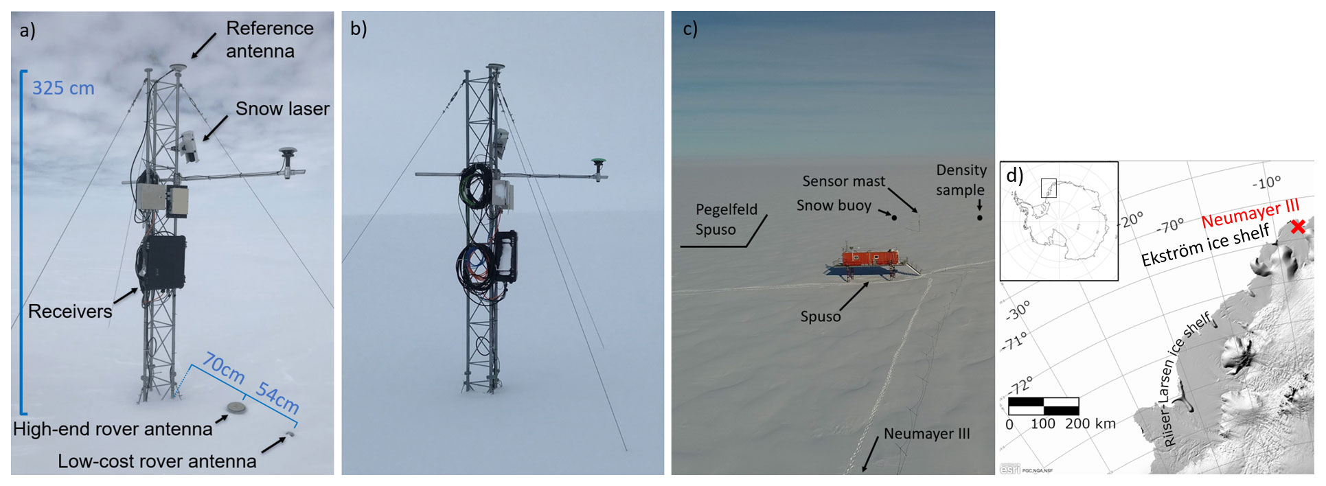
Figure 1(a) The GNSS-RR setup consists of one GNSS reference antenna and two GNSS rover antennas placed on the firn surface (21 November 2021). The rover antennas are physically connected to the sensor mast via a lateral boom (hidden below the snow surface). (b) GNSS-RR setup with both rover antennas already covered by the accumulated snow (23 November 2021). (c) Situation of the test site. (d) Location of the test site at the Ekström ice shelf, Dronning Maud Land, Antarctica (modified from Jakobs et al., 2019).
The GNSS-RR setup consists of a high-end GNSS reference antenna and a high-end and low-cost GNSS rover antenna placed on the firn surface. The rover antennas are buried by the snow accumulating on top of the antennas (Fig. 1b). It is mandatory that the rover antennas are mechanically connected to the reference antenna when deployed on a moving surface. The physical connection enables the correct separation of the SWE-induced effects and station height changes due to the ice shelf movements in the GNSS parameter estimation, as both parameters are highly collinear with 99.7 % (Steiner et al., 2020). The rover antennas are physically (mechanically) fixed to the sensor mast via another lateral boom. The buried lateral boom is rigid and initially placed on very dense, wind-packed snow. The bending of the arm is thus assumed to be negligible. All antennas are equally oriented towards north, and antenna calibration files are applied in the GNSS processing to minimize the antenna-phase center offset and variation effects on the results. Note that the data from a second GNSS reference antenna, mounted on a lateral boom to the sensor mast (Fig. 1a), are not used in the present study.
Table 1Specifications of the deployed high-end and low-cost multifrequency and multisystem GNSS sensors (LeicaGeosystems, 2023a, b; Ublox, 2023; Emlid, 2023). Raspberry Pi (RaspberryPi, 2023) is used for remote control and data transfer of the low-cost receiver.
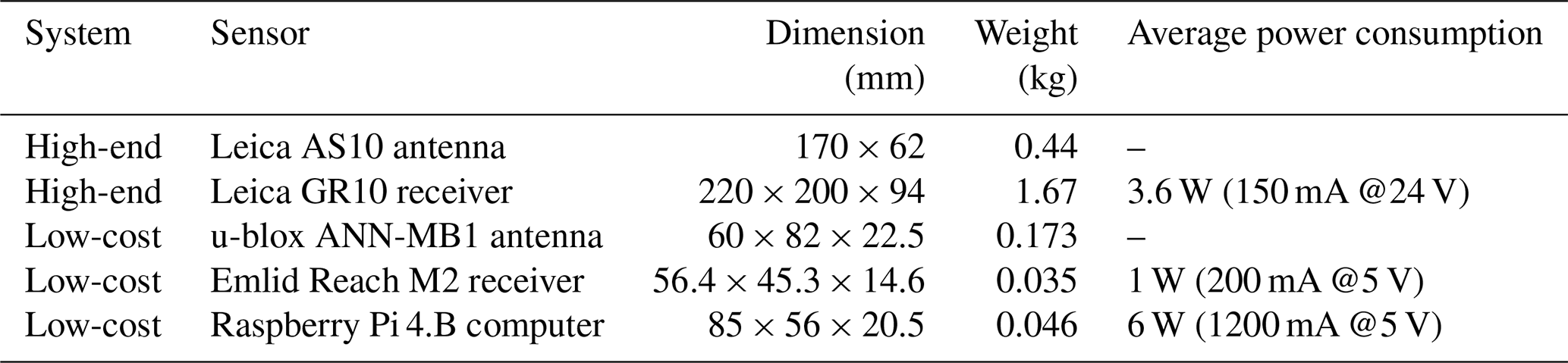
The specifications of the deployed GNSS-RR system are summarized in Table 1. A Raspberry Pi computer is used for remote control and data transfer of the low-cost receiver. The GNSS-RR system collects multifrequency and multisystem (GPS, GLONASS, and Galileo) GNSS signals. The GNSS antenna mounted on top of the sensor mast serves as a GNSS reference for differential processing and, additionally, tracks reflected GNSS signals (1 Hz sampling rate) from the surrounding snow surfaces. The buried GNSS antennas collect refracted GNSS signals (30 s sampling interval), influenced by the accumulated snow above the antennas, from all elevation angles. Power and Ethernet supply is provided by the Spuso which is connected to the Neumayer III station.
2.2 Reference data
Ground truth data for snow deposition and erosion (snow accumulation) are provided with a 1 min sampling interval by a laser distance sensor (Jenoptik SHM30) from the same sensor mast (Schmithüsen, 2023). The laser observations are filtered by a moving median over 24 h to remove outliers and resampled to 15 min to match the temporal resolution of the GNSS-derived results. The nearby (distance ≈ 20 m) snow buoy observations (Nicolaus et al., 2021; Grosfeld et al., 2016), consisting of four sonic ranges (MaxBotix HRXL-MaxSonar-WR3), are furthermore used for reference. Additional ground truth data are provided weekly by 16 accumulation stakes from the nearby “Pegelfeld Spuso” (distance ≈ 200 m). Monthly manual snow accumulation, SWE, and snow density observations from the upper layer (first meter) are taken from the “density sample location” (distance ≈ 50 m) at the same test site (Fig. 1c). A relative uncertainty of 10 % is added as an error bar in all plots to indicate the general accuracy of such manual observations. Continuous snow accumulation data from the laser distance sensor are, additionally, converted to SWE by linearly interpolating the monthly density observations to enable an accuracy estimate for the GNSS-RR-derived SWE time series.
A combined GNSS-RR method, using reflected and refracted GNSS signals (Fig. 2), is applied and investigated regarding its potential for simultaneous, continuous, and accurate estimation of snow accumulation, SWE, and snow density.
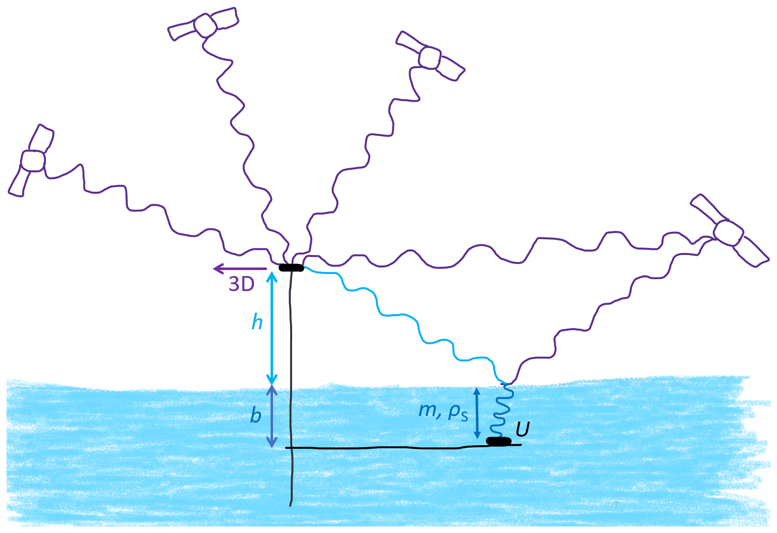
Figure 2Schematic overview of the GNSS-RR measurement principle applied on a moving surface. Direct (purple), reflected (light blue), and refracted (dark blue) GNSS signals are collected to estimate snow accumulation (b), SWE (m), and the density of snow (ρs) above a buried GNSS rover antenna. U is the rover up coordinate, and h is the height difference of the GNSS base antenna to the reflective surface. The three-dimensional antenna movement is illustrated as 3D.
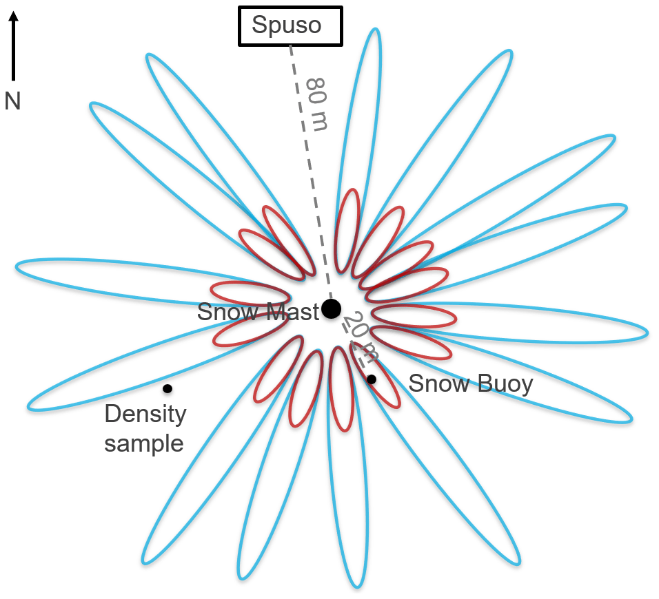
Figure 3Fresnel reflection ellipses illustrating the area of received reflected GNSS signals around the GNSS reference antenna for 5∘ (blue) and 30∘ (red) elevation angles.
3.1 GNSS reflectometry for snow accumulation estimation
In situ snow accumulation (deposition and erosion) is estimated using ground-based GNSS reflectometry (e.g., Jin and Najibi, 2014; Larson et al., 2009). Direct GNSS signals and GNSS signals reflected off a snow/firn surface are analyzed in order to measure the difference in height h between the GNSS reference antenna and the reflective surface. The influence of the reflected signals on the signal strength depends on the path extension, with respect to the direct signals. The overlay of the direct and reflected GNSS signals creates an interference pattern of the signal strengths when satellites move across the sky. The frequency f of these multipath oscillations is related to h (with λ being the GNSS wavelength of the observed satellite system from 18–26 cm) as follows:
The snow accumulation b is given by the change in height (Δh) over time. Figure 3 shows that the area around the GNSS reference antenna, used to estimate snow accumulation, is determined by the first Fresnel reflection ellipses for the experimental setup. The size of these ellipses depends on the height of the reference antenna above the surface and the analyzed incident angles.
The 1 Hz GNSS reference data are post-processed by using the open-source gnssrefl package from Larson (2021). The best results are achieved by selecting GPS, GLONASS, and Galileo second frequencies within an elevation range of 5–30∘. The reflector height was set from 2–8 m to allow automated processing, which is independent of regular sensor mast extensions of approximately 3 m. Distracting low-elevation signals, bending around or reflecting off the nearby Spuso, are excluded based on their azimuthal range. The outliers in the snow accumulation results are removed using a statistical threshold based on the standard deviation (3σ). The resulting time series is filtered by a moving median over 24 h. The derived results are resampled to 15 min values to enable the combination with the SWE estimates from GNSS refractometry.
3.2 GNSS refractometry for SWE estimation
The GNSS refractometry method based on the biased “Up component” (Steiner et al., 2022) is applied to in situ SWE estimation. The signals received by an antenna buried underneath the snowpack are delayed while propagating in a snow/firn layer. These delays cause the estimated antenna position to be biased, especially the vertical up (height) component U. The resulting height deviation from a phase-based differential GNSS position estimation provides information on the change in SWE (i.e., snow mass change δm), as both parameters are highly collinear with 99.7 % (Steiner et al., 2020):
The δm above the buried rover antenna can, thus, be estimated based on the change in the estimated up component δU (Eq. 2) of the rover coordinate. Equivalently, the up component of the derived GNSS baseline between both antennas could be used directly. In contrast to previous GNSS refractometry studies, the present setup is situated on a fast-moving surface. The correlation between the influence of snow on the GNSS signal delay and the ground movement is considered in the experimental setup (Sect. 2.1) by physically connecting the rover to the base antenna. If the physical height difference between the two antennas were not known and fixed, the SWE parameter could not be separated from the station height due to the changes caused by the ground movement.
The GNSS refractometry data are post-processed using the open-source GNSS processing software, RTKLIB version 2.4.3 b34 (Takasu, 2009). Although multisystem data are collected, the best results are achieved by only using multifrequency GPS data for the SWE estimation. For the processing, 7 to 13 GPS satellites are generally available on site. The additional use of Galileo and GLONASS observations increased the number of unusable solutions in the case of our experiment. This is assumed to be caused by the applied processing software, which was initially coded for GPS only and extended for multi-GNSS systems afterward, potentially leading to problems in nonstandard GNSS applications. Processing intervals of 15 min are applied to the differential GNSS processing with a very short baseline (3–6 m). All elevation observations are used to enhance the SWE estimation accuracy (Steiner et al., 2020). The reference coordinate is not fixed due to the ground movement, but it is selected automatically from each day's navigation position (available in the resulting RINEX observation file header) to guarantee an adequate initial coordinate for the differential processing. Similar to the snow accumulation estimation, the outliers in the SWE results are removed using the 3σ statistical threshold. The 15 min SWE time series is filtered by a moving median over 24 h.
3.3 Combined GNSS-RR for snow density estimation
The in situ snow density ρs is derived by combining the individual results from GNSS reflectometry (snow accumulation b) and refractometry (SWE m):
The resulting daily densities, that are lower than the density of new snow (50 kg m−3) or higher than the density of firn (830 kg m−3), are removed for plausibility. The SWE and snow density are determined as an average over an area of a few square meters around the antenna, depending on the height of the snow above the buried rover antennas, snow wetness, and signal incidence angles.
Combined GNSS-RR estimation results for snow accumulation (Sect. 4.1), SWE (Sect. 4.2), and snow density (Sect. 4.3) are presented for the fast-moving Ekström ice shelf in Antarctica. The results are compared with ground truth data from the same test site (Sect. 2.1).
4.1 Snow accumulation
Figure 4a illustrates the results from GNSS reflectometry, using the open-source gnssrefl package, for the end of November 2021 to April 2023. All snow accumulation estimates (transparent steel blue area) are overlaid by the median-filtered snow accumulation estimates (steel blue line). The snow accumulation varies significantly (standard deviation of 23 cm) over the reflection area, which covers a radius of up to 80 m around the reference antenna (Fig. 3). The variation is predominantly caused by strong winds, leading to spacial and temporal heterogeneity in snow deposition and erosion within the test site. The estimated snow accumulation is directly compared with the reference data of the laser distance sensor (dark blue) from the same mast. The GNSS-derived accumulation shows a very high level of agreement with the laser observations for the first weeks in November/December 2021, with differences around 2 cm (Fig. 4b). The storms in mid-December 2021 led to a strong increase in snow accumulation (up to 50 cm), as observed by the laser sensor. In contrast, the increase in accumulation derived by GNSS reflectometry is significantly less, with 32 cm for the same time period. This difference is in the order of the horizontal homogeneity of the snow surface and may be explained by the different footprints of the two methods. This rationale is supported by comparable extreme values of the GNSS estimate around this time. Note that the laser distance sensor broke down at the beginning of October 2022 and was replaced at the end of December 2023, leading to a lack of data for this time period.
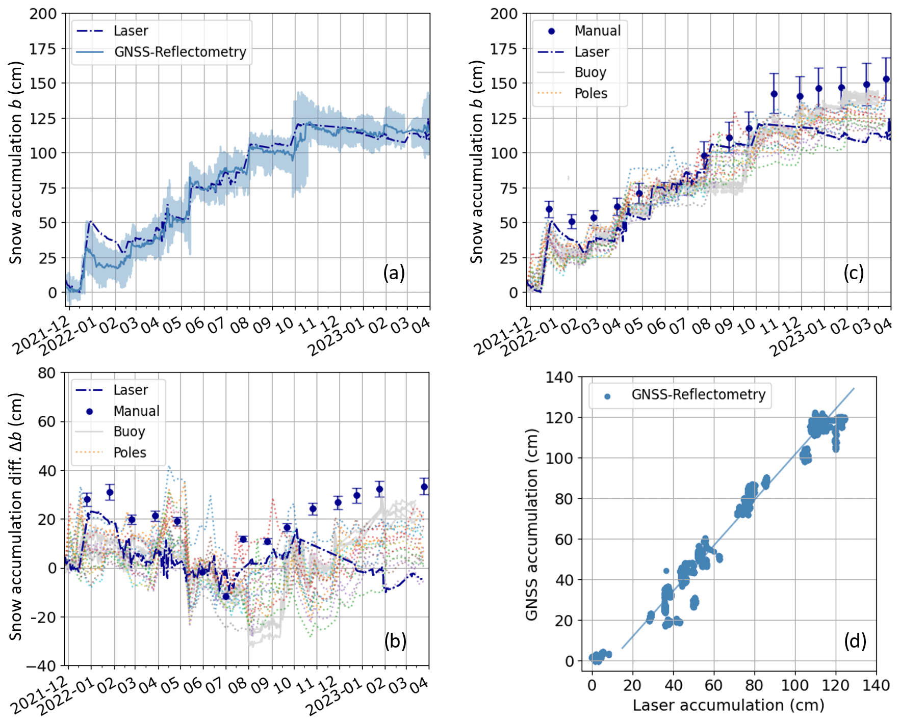
Figure 4(a) Time series of median GNSS-reflectometry-derived snow accumulation (steel blue line) overlaid by all accumulation estimates (steel blue area) and compared with the laser observations (dark blue). (b) Differences between all reference sensor observations and the median GNSS reflectometry estimates and (c) visual comparison of all available reference data for November 2021 to April 2023. A relative uncertainty of 10 % is added as an error bar to the manual observations. (d) Correlation of GNSS reflectometry with the laser accumulation (see also Table 2).
Additional reference data (Sect. 2.2) are available for comparison (Fig. 4c) from the nearby manual observations (dark blue dots), snow buoy (gray curves), and 16 stake observations (colored dotted lines). A strong variation in snow accumulation is observed among all the reference sensor's data, with similar magnitudes as the difference in accumulation between the GNSS-derived results and the laser observations.
The accumulation observations decrease significantly after the mid-December event and last until February 2022. The GNSS-derived accumulation closely follows the trend observed by the laser distance reference sensor for the rest of the observation period. The differences between the GNSS results and the laser vary around 35 cm. The overall results have a root mean square error (RMSE) of 8.5 cm (Table 2), when compared with the laser observations.
The accumulation results are compared to the laser observations in Fig. 4d based on a linear regression. The snow accumulation estimated by GNSS reflectometry is highly correlated to the laser observations, with Pearson cross correlation coefficients (r) of 0.98. The offsets induced by the snow deposition and erosion heterogeneity are visible in the linear fit. Table 2 lists the regression coefficients.
Table 2Regression coefficients for the comparison of the snow accumulation estimated by the GNSS reflectometry (GNSS-R) and observed by the laser for 2021–2023. The linear regression fit is defined by the offset (o) and the slope (a). The number of samples is given by n.
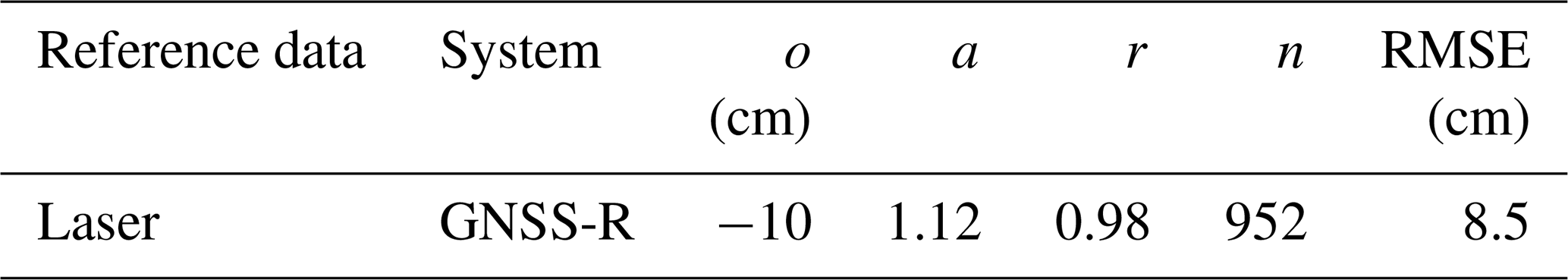
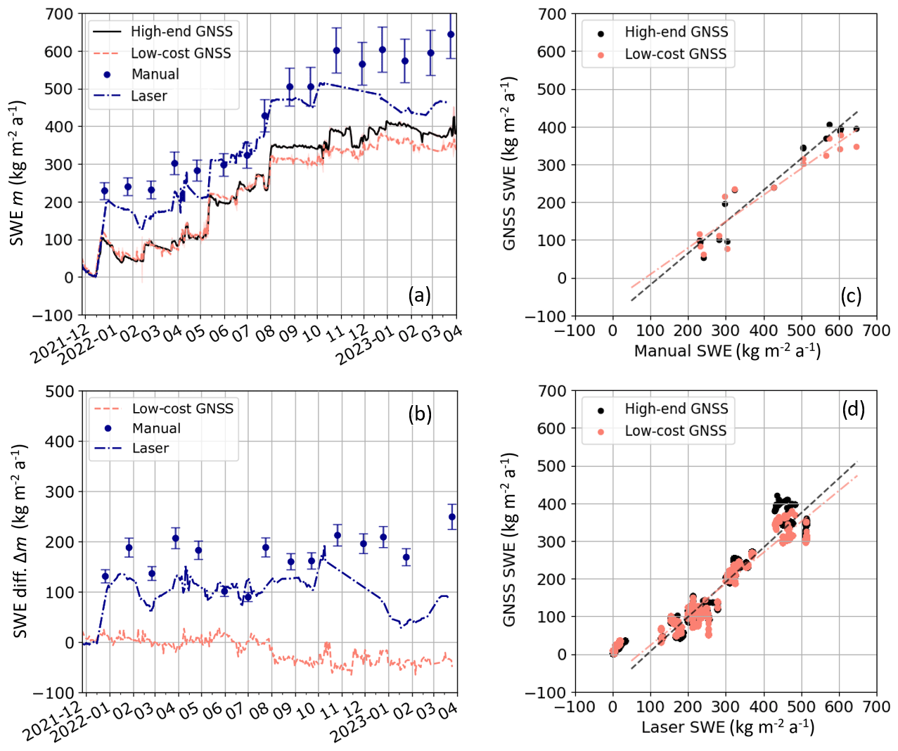
Figure 5(a) Time series of median of GNSS-refractometry-derived SWE for the high-end and low-cost systems, compared with reference data for November 2021 to April 2023. A relative uncertainty of 10 % is added as an error bar to the manual observations. (b) Differences between the low-cost GNSS refractometry estimates, manual reference sensor observations, and laser reference sensor observations and the high-end GNSS refractometry estimates. Correlation between (c) manual and (d) laser observations (see also Table 3).
4.2 Snow water equivalent
The GNSS-refractometry-derived SWE is median filtered, and Fig. 5a shows the high-end (black) and low-cost (orange) system from the end of November 2021 to April 2023. The median SWE time series is overlaid by the noise (standard deviation per day, transparent black and orange) of the 30 s SWE estimation before filtering (3 kg m−2 a−1 for the high-end and 6 kg m−2 a−1 for the low-cost system). The standard deviation of the median-filtered SWE, resulting from the high-end and low-cost system, is 2 kg m−2 a−1. Both of the GNSS-derived SWE estimates strongly agree with each other until August 2022, with noisier results from the low-cost system. The differences between the high-end and low-cost system increase afterward, where the low-cost results start to underestimate the SWE up to 64 kg m−2 a−1 (Fig. 5b). All possible error sources related to the GNSS refractometry processing (antenna height, base coordinate, antenna calibration parameters, WGS84 reference ellipsoid, satellite availability, and signal strengths) were checked. As GNSS refractometry is a relative observation method between the base and rover antenna, the processing is consistent for all data epochs and receivers. There was no change in the satellite signatures; therefore, we could exclude all such error sources. Since the offset is sudden and affects the receiver height, we assume a change in the effective physical height of the low-cost antenna. The antenna is screwed on the submerged lateral boom via a small vertical balise bar. Due to the overlying pressure of the snowpack and the cold, it could be possible that the screw had become loose, and the antenna sank a few centimeters into the underlying snow.
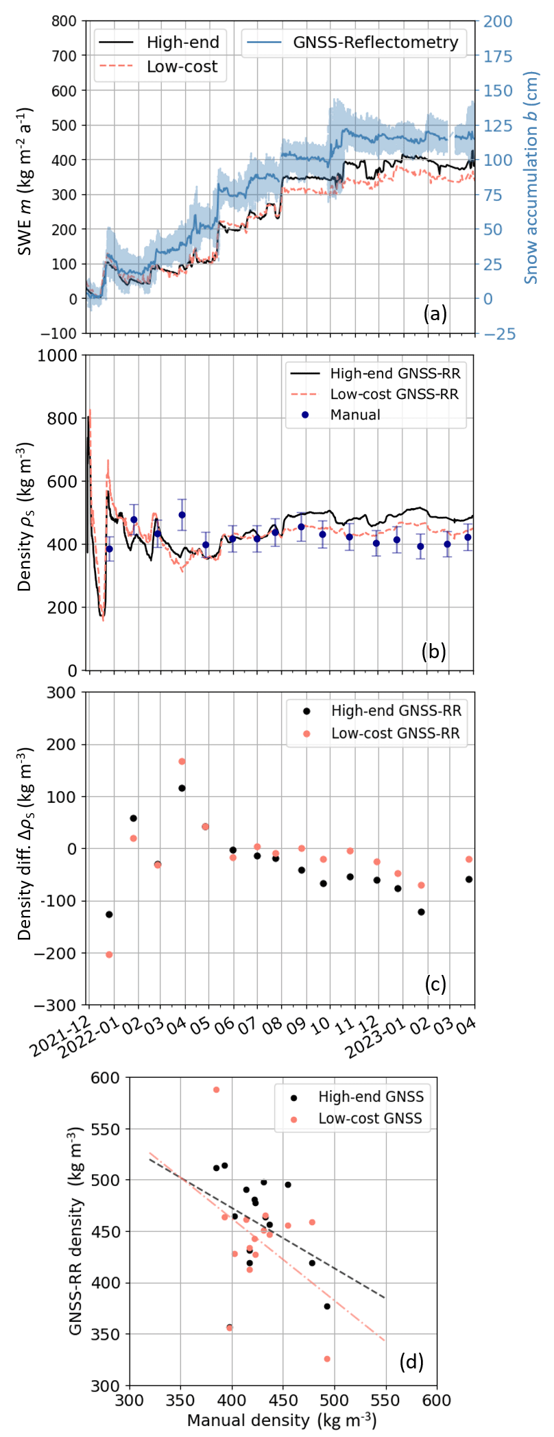
Figure 6(a) Comparison of GNSS-reflectometry- and refractometry-derived accumulation and SWE time series. (b) GNSS-RR-derived density time series from the high-end and low-cost system compared to manual observations. (c) Differences between and (d) correlation of GNSS-RR density estimates with manual observations.
The derived SWE is directly compared with the nearby manual reference observations (blue dots). A relative uncertainty of 10 % is added as an error bar to the manual observations. An additional reference, with a higher temporal resolution, is provided by the laser distance observations (dashed blue line). The observed snow accumulation data are, thereby, converted to SWE by linearly interpolating the available manual density measurements (Sect. 2.2). Note that the laser distance sensor broke down at the beginning of October 2022 and was replaced at the end of December 2022, leading to a lack of data for this time period.
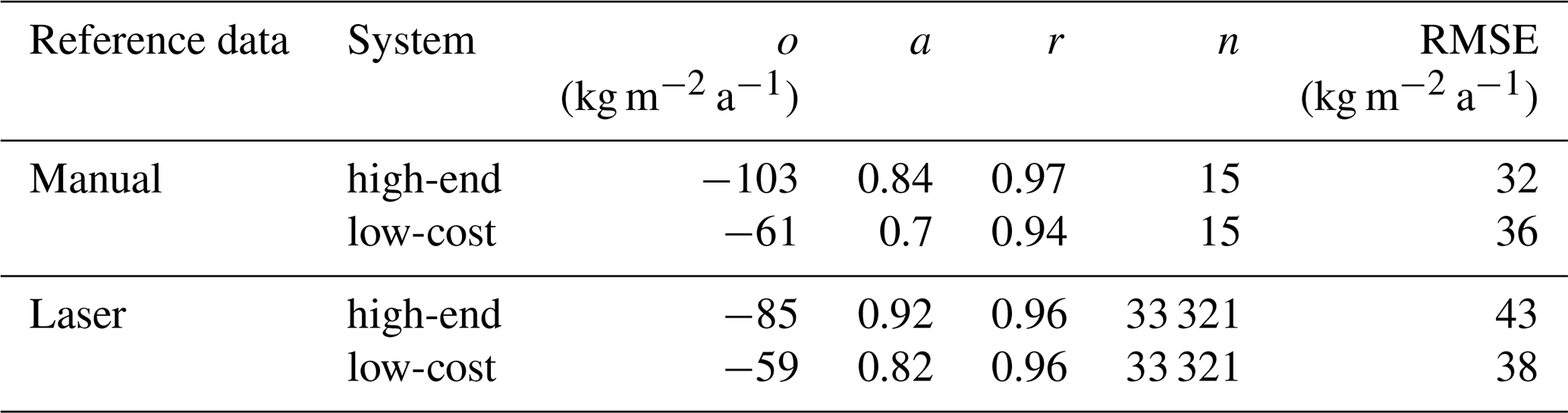
The GNSS-refractometry-derived SWE shows a very high level of agreement with the laser reference observations for the first weeks of the diminishing snow in November/December 2021, with differences around ±5 kg m−2 a−1 (Fig. 5b). As is already visible in the snow accumulation results (Sect. 4.1), heavy snowfall increased the SWE up to 200 kg m−2 a−1 (observed by the laser sensor) or even 230 kg m−2 a−1 (observed manually) in mid-December 2021. The increase in SWE derived by GNSS refractometry is significantly less, with 105 kg m−2 a−1 for the same time period. The reason is similar to the reason for the difference observed in the snow accumulation results, and it is caused by the heterogeneity of the snow deposition and erosion within the test area. The GNSS-refractometry-derived SWE closely follows the trend of the laser observations after mid-December. The differences in the laser data vary within 193 kg m−2 a−1. The present deviations (up to 204 kg m−2 a−1) are higher, when compared with the manual observations. The results from the high-end system have an RMSE of 32 kg m−2 a−1 to the manual and 43 kg m−2 a−1 to the laser observations (Table 3). The results from the low-cost system have an RMSE of 36 kg m−2 a−1 to the manual and 38 kg m−2 a−1 to the laser observations.
The SWE results are compared with the reference observations in Fig. 5c and d, using a linear regression. The SWE estimates derived from GNSS refractometry are highly correlated to the manual and laser observations, with r between 0.94 and 0.97 (Table 3). The offsets induced by the snow deposition and erosion heterogeneity are visible in the linear fit. Table 3 lists the regression coefficients.
Table 3Comparison of the SWE estimated by GNSS refractometry and observed by each reference sensor for 2021–2023. The linear regression is defined by the offset (o) and the slope (a). The number of samples is given by n.
4.3 Snow density
Combining the median-filtered, GNSS-derived results for snow accumulation and SWE leads to estimates of snow density (temporal resolution of 15 min) for the observed area. Figure 6a illustrates the SWE and accumulation results from GNSS reflectometry and refractometry, respectively. Snow accumulation decreases in November and December 2021, followed by snow deposition in mid-December 2021. Generally, snow deposition and erosion dominate the change in SWE. It seems, however, that the snow settles during August and September 2022, after an increase in accumulation, as the deposited snow decreases, while the SWE stays nearly constant.
Figure 6b shows the combined GNSS-RR-derived snow density from the high-end and low-cost system from the end of November 2021 to April 2023. Additionally, Fig. 6b shows the manual density observations and their accuracy, for reference. The GNSS-RR-derived densities are calibrated to the manual observation of 24 July 2022. Approximately 1 m of snow accumulated on top of the buried GNSS antennas on that day, which enables a correct match with the manual density observation of the upper 1 m layer (top 1 m), for better comparison. The results from the high-end and low-cost GNSS-RR method agree well with each other until August 2022. The low-cost system yields lower densities after August 2022 compared with the high-end results. Although the low-cost results seem to fit better with the manual density observations after August 2022, the lower density estimates are caused by the underestimated low-cost SWE results and error propagation, when calculating the density. The high-end GNSS-RR-derived estimates yield higher densities after August 2022 compared with the manual observations, with an increasing trend (Fig. 6c). The accumulation on top of the buried GNSS antennas exceeds 1 m after August 2022. The larger amount of snow above the buried antennas (b > 1 m) could lead to the illustrated increase in the density observations, when compared with the manual observation of the top 1 m of the snowpack.
Strong variations in the derived density time series are present until March 2022 for both systems, when compared with the manual reference observations. During this time interval, the snow accumulation above the buried antennas was quite shallow (below 20 cm), and, consequently, the estimated SWE values were very low. As the GNSS-derived SWE estimation uncertainties are independent of the magnitude of the SWE itself, large density variations can result from small SWE values. Once the snow above the antennas is thicker, the combined GNSS-RR method enables feasible density estimates, which agree well with the manual reference observations.
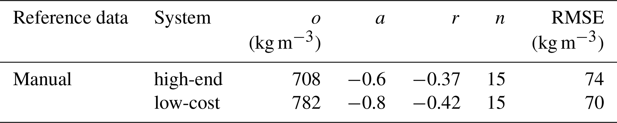
The high-end and low-cost density results are compared with the manual reference observations in Fig. 6d, using a linear regression. The GNSS-RR-derived density estimates show a low negative correlation to the manual observations, with r being −0.37 for the high-end and −0.42 for the low-cost system (Table 4). These results are highly influenced by the strong variation in the first months due to the shallow snowpack above the buried GNSS antennas. Table 4 lists the regression coefficients.
Table 4Comparison of the GNSS-RR-derived snow or firn density with the manual observations for 2021–2023. The linear regression is defined by the offset (o) and the slope (a). The number of samples is given by n.
Generally, the GNSS-RR-derived snow accumulation, SWE, and density estimates agree well with the reference sensor's data over the evaluated period of 16 months. All reference sensors measure on a point-wise, local scale and are situated at different locations within the experimental site (Sect. 2.2), with distances up to 200 m (stakes) from the GNSS-RR installation. Although the laser reference sensor is deployed on the same sensor mast as the GNSS-RR system, the measurement areas (spatial footprints) differ significantly. The laser observation is a point measurement, whereas the spatial footprint of GNSS refractometry depends on the depth and permittivity of the accumulated snowpack above the buried GNSS antenna and the observed GNSS incidence angles. In the present case of using all GNSS observations from all available incidence angles, an area up to 2 m in diameter is observed for a 1 m dry snowpack above the buried GNSS antenna. GNSS reflectometry collects reflections even over a much larger area, with a diameter up to 80 m around the GNSS base antenna for the analyzed incidence angles of 5–30∘ and antenna heights up to 3 m above the surface. The strong variation in snow accumulation, caused by the heterogeneity in snow deposition and erosion over the observation area, is, therefore, visible in all sensory observations due to the different sensor locations and spatial footprints. Due to the small footprint and high accuracy of the laser (5 mm; G. Lufft Mess- und Regeltechnik GmbH, 2015) and snow buoy (1 mm; Nicolaus et al., 2021) measurements, these accumulation observations are highly sensitive to local variations in surface roughness. The predominant wind is coming from the east, leading to enhanced snow accumulation on the west side, right behind the sensor mast, where the laser footprint is located. As the GNSS-RR footprint is much larger, such heterogeneities are filtered out by averaging all observations within the larger area. The GNSS-RR measurement is less sensitive to spatial heterogeneity due to its lower accuracy for accumulation estimation (8.5 cm). Manual observations are generally considered to have an uncertainty of 1 cm but are less spatially and temporally represented. Additionally, point-wise observations are more sensitive to sastrugi, which are formed by the wind-driven erosion of snow and potentially move across the observation area. The observations with a larger footprint are less affected, as such accumulation events are averaged out.
Higher deviations between the GNSS-derived accumulation and SWE estimates, when compared with the laser observations, are present after the strong accumulation event in mid-December 2021. These accumulation and SWE differences are of similar magnitudes to the deviations between all the reference sensor's observations, and they are assumed to be caused by the heterogeneity of the snow deposition and erosion within the test area. The accuracies of SWE observed manually (40 kg m−2) or by GNSS refractometry (30–40 kg m−2) show a similar magnitude for the 1 m deep snowpack, with the highest SWE being around 400 kg m−2. Density observations are, however, less accurate from the combined GNSS-RR (74 kg m−3), when compared with the manual density observations (40 kg m−3) of the observed density range.
A main advantage of the combined GNSS-RR method is the possibility to continuously estimate the snow or firn accumulation, SWE, and density automatically at a low cost, allowing us to support the understanding of surface-related processes, such as firn densification processes, in future studies. The combined GNSS-RR method can, therefore, support the identification and interpretation of the dominating surface-related snow process, especially in the cases of decreasing snow surface levels. It is not possible to distinguish between snow erosion, compaction, and sublimation processes with pure accumulation observations, such as laser, buoy, or stake observations. This interpretation can be supported thanks to the simultaneous observation of accumulation, SWE, and density with a high temporal resolution. The decreasing snow accumulation observed together with the decreasing SWE can indicate snow erosion or melting (for example, end of December 2021 and January 2022, Fig. 6a). The decreasing snow accumulation together with a stable SWE could be interpreted as snow settling, which is dominated by compaction and sublimation processes (for example, August and September 2022, Fig. 6a, b).
The GNSS-RR system is a promising method as the system is of a small size and cost, easy to deploy, needs little maintenance, is passive and nondestructive, and enables automatic observations independent of weather conditions. Besides heightening the sensor mast to compensate for yearly accumulating snow, no access is required during the measurement period, which simplifies the application in remote polar environments. Power supply can, thereby, be a limiting factor. Point-wise observations are additionally limited by their representation in the spatial variability and, thus, the understanding of SMB-related processes on a larger scale. Further studies need to investigate the combined GNSS-RR method in more detail based on multiple dispersed stations at different experimental sites.
A minimum amount (20 cm) of snow above the buried GNSS antenna is a prerequisite to achieve reliable results for the density estimation. Previous studies show the feasibility of GNSS refractometry for accurate SWE estimation, even for a very shallow snowpack above the buried antenna (Steiner et al., 2018a). Similar findings were obtained for GNSS reflectometry (e.g., Larson et al., 2009). Here, it is assumed that the strong deviations in density estimation in the first months are due to the high heterogeneity within the test site. In combination with a very shallow snowpack, this leads to high relative uncertainties of the individual snow accumulation and SWE estimates. Consequently, the uncertainties in the density estimation, derived from a combination of these input values, are propagated, leading to less reliable density estimates. This could be avoided by installing the GNSS rover antennas approximately 20 cm below the surface at the beginning. In this case, the snow accumulation, SWE, and the density above the buried antenna need to be measured to be able to calibrate the initial observation.
Another limitation is the inclination of the application surface, as the height component of the GNSS baseline between the base and rover antennas must be fixed. The system needs to be deployed in a very stable setup. Otherwise, for example, if the system were to be mounted on a tripod on a glacial surface with high surface melt, the setup could get tilted, which changes the height difference between the base and rover. This change cannot be separated from the influences due to snow above the buried GNSS antenna. If the system setup is prone to tilting and the relative height difference between the reference and rover antennas cannot be ensured, installing an additional tiltmeter could make sense to enable us to monitor the physical baseline height component. Power monitoring could also be added for remote self-sufficient locations.
The present study illustrates the potential of a combined GNSS-RR method for the accurate, simultaneous, and continuous estimation of in situ snow accumulation, SWE, and snow density time series. The combined GNSS-RR method was successfully applied on a fast-moving, polar ice shelf. Snow accumulation results could be accurately determined using reflected GNSS observations. SWE was successfully estimated with a high temporal resolution (15 min), using GNSS refractometry based on the biased up component. A high level of agreement with available reference data was achieved for both individual methods. Combining results from both methods illustrated the potential of using a combined GNSS-RR approach for deriving in situ snow densities with a 15 min resolution. A minimum amount (20 cm) of snow above the buried GNSS antenna was proven to be a prerequisite to achieve reliable results.
The combined GNSS-RR approach could be highly advantageous for a continuous quantification of ice sheet and glacier SMB. The accumulation change in snow and firn can be derived using one single method by simultaneously estimating the snow accumulation, SWE, and density with a high temporal resolution. Snow-hydrological modeling predicts local snow distribution, snow drift, and snowmelt, whereas climate models are used to predict mass balance changes on a regional scale. Both types of models could profit from such derived field measurements. The combined approach could also supplement or replace manual in situ data collection, leading to reduced expenses and enhanced temporal and spatial resolutions of the retrieved snow characteristics. Besides the application to a polar ice sheet, ice streams, and ice shelves, the simultaneous retrieval of these snow characteristics in seasonal snow additionally supports public institutions, private companies, and environmental offices by providing fundamental data for managing the drinking and irrigation water supply and hydro-power energy supply or assessing flood and avalanche risks. Point-wise observations are, however, limited by their representativeness in the spatial variability and, thus, the understanding of SMB-related processes on a larger scale.
Future research could further investigate the potential of linking such derived in situ density time series, available with a high temporal resolution, to extensive surface-elevation observations (such as laser or radar altimetry) for improved SMB estimation on a larger scale. This could allow more reliable assessments and enhanced understanding of the contribution of SMB-related processes driving the future rise in sea level.
Python code for preprocessing, processing, analyzing, and visualizing the GNSS-RR data is provided on GitHub (https://github.com/lasteine/GNSS_RR.git, last access: 20 November 2023; DOI: https://doi.org/10.5281/zenodo.10135417, Steiner, 2023). Collected and analyzed multifrequency and multisystem GNSS data have been made publicly available at PANGAEA (https://doi.org/10.1594/PANGAEA.958973, Steiner et al., 2023).
Conceptualization: LS, JW, and OE; fieldwork: LS and OE; methodology: LS and JW; analysis and investigation: LS; reference data and accessibility to the Meteorological Observatory Neumayer: HS; draft preparation: LS; visualization: LS; glaciological know-how, expedition expertise, and scientific coordination: OE.
At least one of the (co)authors is a member of the editorial board of The Cryosphere. The peer-review process was guided by an independent editor, and the authors also have no other competing interests to declare.
Publisher's note: Copernicus Publications remains neutral with regard to jurisdictional claims made in the text, published maps, institutional affiliations, or any other geographical representation in this paper. While Copernicus Publications makes every effort to include appropriate place names, the final responsibility lies with the authors.
This project was strongly supported by many collaborators, who enabled a successful outcome thanks to their valuable support and inputs.
The authors would like to thank Andreas Frenzel, engineer at AWI, for the valuable technical support in the experimental setup design stage. We would also like to thank Markus Ramatschi (GFZ) for the expertise and preliminary work related to a pre-existing GNSS-RR system at the same sensor mast which simplified our system setup. We also thank Bernhard Richter, Vice President of Geomatics at Leica Geosystems AG, for supporting this project by providing the high-end GNSS equipment and support as part of the Hexagon's sustainability strategy. A big thank you is expressed to the logistics experts, Stefanie Klüver (AWI) and Isabelle Rümmele (Leica Geosystems AG), for their valuable support with customs regulations regarding the shipping of the high-end GNSS equipment from Switzerland to the EU. Huge thanks are given to Martin Petri and Norbert Anselm, observation to archive (O2A; Koppe et al., 2015) at AWI, for providing profound IT support, server infrastructure at Neumayer III, data transfer to Germany, and the framework for the project dashboard for online data checking. We thank Peter Köhler, senior scientist at AWI, for the great help during the GNSS-RR system setup in Antarctica. Special thanks are given to the overwintering team at Neumayer III (Linda Ort, Theresa Thoma, Paul Ockenfuss, Hannes Keck, and Nellie Wullenweber) for the on-site support, fieldwork, and reference data observation. We thank Rolf Weller for the accessibility to the air chemistry observatory at Neumayer III. Lastly, but not least, a big thank you is expressed to the expedition organizers and all the team members for the selection of, contribution to, and support of this project as part of the German Antarctic expedition in 2021/22. Autonomous snow buoy measurements from November 2021 to April 2023 were obtained from https://www.meereisportal.de (last access: 22 May 2023) (grant: REKLIM-2013-04).
Ladina Steiner was granted a Postdoc.Mobility fellowship (P400P2_199328/1) from the Swiss National Science Foundation. The research was also supported by the Helmholtz POF IV initiative.
This paper was edited by Arjen Stroeven and reviewed by Ian Brown and Maaria Nordman.
Arslan, A. N., Tanis, C. M., Metsaemaeki, S., Aurela, M., Boettcher, K., Linkosalmi, M., and Peltoniemi, M.: Automated webcam monitoring of fractional snow cover in northern boreal conditions, Geosciences, 7, 55, https://doi.org/10.3390/geosciences7030055, 2017. a
Beaumont, R.: Hood pressure pillow snow gage, J. Appl. Meteorol., 4, 626–631, 1965. a
Capelli, A., Koch, F., Henkel, P., Lamm, M., Appel, F., Marty, C., and Schweizer, J.: GNSS signal-based snow water equivalent determination for different snowpack conditions along a steep elevation gradient, The Cryosphere, 16, 505–531, https://doi.org/10.5194/tc-16-505-2022, 2022. a
Davison, B. J., Hogg, A. E., Rigby, R., Veldhuijsen, S., van Wessem, J. M., van den Broeke, M. R., Holland, P. R., Selley, H. L., and Dutrieux, P.: Sea level rise from West Antarctic mass loss significantly modified by large snowfall anomalies, Nat. Commun., 14, 2041–1723, https://doi.org/10.1038/s41467-023-36990-3, 2023. a
Eisen, O., Frezzotti, M., Genthon, C., Isaksson, E., Magand, O., van den Broeke, M. R., Dixon, D. A., Ekaykin, A., Holmlund, P., Kameda, T., Karlöf, L., Kaspari, S., Lipenkov, V. Y., Oerter, H., Takahashi, S., and Vaughan, D. G.: Ground-based measurements of spatial and temporal variability of snow accumulation in East Antarctica, Rev. Geophys., 46, RG2001, https://doi.org/10.1029/2006RG000218, 2008. a
Emlid: Emlid Reach M2 multi-band receiver specifications, https://store.emlid.com/eu/product/reachm2/ (last access: 17 April 2023), 2023. a
Frey, O., Werner, C. L., Caduff, R., and Wiesmann, A.: Tomographic profiling with Snowscat within the ESA Snowlab Campaign: Time series of snow profiles over three snow seasons, in: IGARSS 2018–2018 IEEE International Geoscience and Remote Sensing Symposium, 6512–6515, https://doi.org/10.1109/IGARSS.2018.8517692, 2018. a
Gardner, A. S., Moholdt, G., Cogley, J. G., Wouters, B., Arendt, A. A., Wahr, J., Berthier, E., Hock, R., Pfeffer, W. T., Kaser, G., Ligtenberg, S. R. M., Bolch, T., Sharp, M. J., Hagen, J. O., van den Broeke, M. R., and Paul, F.: A reconciled estimate of glacier contributions to sea level rise: 2003 to 2009, Science, 340, 852–857, https://doi.org/10.1126/science.1234532, 2013. a
G. Lufft Mess- und Regeltechnik GmbH: SHM 30 Snow Depth Sensor User Manual, https://www.lufft.com/de-de/downloads/ (last access: 7 November 2023), 2015. a
Grosfeld, K., Treffeisen, R., Asseng, J., Bartsch, A., Bräuer, B., Fritzsch, B., Gerdes, R., Hendricks, S., Hiller, W., Heygster, G., Krumpen, T., Lemke, P., Melsheimer, C., Nicolaus, M., Ricker, R., and Weigelt, M.: Online sea-ice knowledge and data platform, https://doi.org/10.2312/polfor.2016.011, 2016. a
Gschwend, F.: Schneehöhenmessung mit GPS, masters thesis, Institute of Geodesy and Photogrammetry, ETH Zurich, https://doi.org/10.13140/RG.2.2.12948.35202, 2012. a
Gugerli, R., Salzmann, N., Huss, M., and Desilets, D.: Continuous and autonomous snow water equivalent measurements by a cosmic ray sensor on an alpine glacier, The Cryosphere, 13, 3413–3434, https://doi.org/10.5194/tc-13-3413-2019, 2019. a
Gutmann, E. D., Larson, K. M., Williams, M. W., Nievinski, F. G., and Zavorotny, V.: Snow measurement by GPS interferometric reflectometry: an evaluation at Niwot Ridge, Colorado, Hydrol. Process., 26, 2951–2961, https://doi.org/10.1002/hyp.8329, 2012. a
Hanna, E., Huybrechts, P., Steffen, K., Cappelen, J., Huff, R., Shuman, C., Irvine-Fynn, T., Wise, S., and Griffiths, M.: Increased runoff from melt from the Greenland Ice Sheet: A response to global warming, J. Climate, 21, 331–341, https://doi.org/10.1175/2007JCLI1964.1, 2008. a
Heilig, A., Eisen, O., MacFerrin, M., Tedesco, M., and Fettweis, X.: Seasonal monitoring of melt and accumulation within the deep percolation zone of the Greenland Ice Sheet and comparison with simulations of regional climate modeling, The Cryosphere, 12, 1851–1866, https://doi.org/10.5194/tc-12-1851-2018, 2018. a
Heilig, A., Eisen, O., Schneebeli, M., MacFerrin, M., Stevens, C. M., Vandecrux, B., and Steffen, K.: Relating regional and point measurements of accumulation in southwest Greenland, The Cryosphere, 14, 385–402, https://doi.org/10.5194/tc-14-385-2020, 2020. a, b
Helm, V., Humbert, A., and Miller, H.: Elevation and elevation change of Greenland and Antarctica derived from CryoSat-2, The Cryosphere, 8, 1539–1559, https://doi.org/10.5194/tc-8-1539-2014, 2014. a
Henkel, P., Koch, F., Appel, F., Bach, H., Prasch, M., Schmid, L., Schweizer, J., and Mauser, W.: Snow water equivalent of dry snow derived from GNSS carrier phases, IEEE T. Geosci. Remote, 56, 3561–3572, https://doi.org/10.1109/TGRS.2018.2802494, 2018. a
Jakobs, C. L., Reijmer, C. H., Kuipers Munneke, P., König-Langlo, G., and van den Broeke, M. R.: Quantifying the snowmelt–albedo feedback at Neumayer Station, East Antarctica, The Cryosphere, 13, 1473–1485, https://doi.org/10.5194/tc-13-1473-2019, 2019. a
Jin, S. and Najibi, N.: Sensing snow height and surface temperature variations in Greenland from GPS reflected signals, Adv. Space Res., 53, 1623–1633, https://doi.org/10.1016/j.asr.2014.03.005, 2014. a, b
Johnson, J., Gelvin, A., Duvoy, P., Schaefer, G., Poole, G., and Horton, G.: Performance characteristics of a new electronic snow water equivalent sensor in different climates, Hydrol. Process., 29, 1418–1433, 2015. a
Kinar, N. and Pomeroy, J.: SAS2: the system for acoustic sensing of snow, Hydrol. Process., 29, 4032–4050, 2015. a
King, M. A., Bingham, R. J., Moore, P., Whitehouse, P. L., Bentley, M. J., and Milne, G. A.: Lower satellite-gravimetry estimates of Antarctic sea-level contribution, Nature, 491, 586–589, https://doi.org/10.1038/nature11621, 2012. a
Koch, F., Henkel, P., Appel, F., Schmid, L., Bach, H., Lamm, M., Prasch, M., Schweizer, J., and Mauser, W.: Retrieval of snow water equivalent, liquid water content, and snow height of dry and wet snow by combining GPS signal attenuation and time delay, Water Resour. Res., 55, 4465–4487, https://doi.org/10.1029/2018WR024431, 2019. a
Koppe, R., Gerchow, P., Macario, A., Haas, A., Schäfer-Neth, C., and Pfeiffenberger, H.: O2A: A generic framework for enabling the flow of sensor observations to archives and publications, in: OCEANS 2015 – Genova, 1–6, https://doi.org/10.1109/OCEANS-Genova.2015.7271657, 2015. a
Larson, K. and Small, E.: Snow depth retrievals using L1 GPS signal-to-noise ratio data, IEEE J. Sel. Top. Appl., 9, 4802–4808, 2016. a
Larson, K., Gutmann, E., Zavorotny, V., Braun, J., Williams, M., and Nievinski, F.: Can we measure snow depth with GPS receivers?, Geophys. Res. Lett., 36, L17502, https://doi.org/10.1029/2009GL039430, 2009. a, b, c
Larson, K. M.: kristinemlarson/gnssrefl: First release, Zenodo [code], https://doi.org/10.5281/zenodo.5601495, 2021. a
LeicaGeosystems: Leica Geosystems AG GNSS reference network antenna specifications, https://leica-geosystems.com/en-gb/products/gnss-reference-networks/antennas/leica-as10 (last access: 17 April 2023), 2023a. a
LeicaGeosystems: Leica Geosystems AG GNSS reference network receiver specifications, https://leica-geosystems.com/products/gnss-reference-networks/receivers/leica-gr50-and-gr30 (last access: 17 April 2023), 2023b. a
Leinss, S., Wiesmann, A., Lemmetyinen, J., and Hajnsek, I.: Snow water equivalent of dry snow measured by differential interferometry, IEEE J. Sel. Top. Appl., 8, 3773–3790, https://doi.org/10.1109/JSTARS.2015.2432031, 2015. a
Lenaerts, J. T. M., Medley, B., van den Broeke, M. R., and Wouters, B.: Observing and modeling ice sheet surface mass balance, Rev. Geophys., 57, 376–420, https://doi.org/10.1029/2018RG000622, 2019. a
Limpach, P., Geiger, A., Gschwend, F., Ruesch, M., and Dawes, N.: Monitoring of snow height and snow water equivalent with GPS, EGU General Assembly, Vienna, Austria, EGU2013-11920-2, 2013. a
Markus, T., Neumann, T., Martino, A., Abdalati, W., Brunt, K., Csatho, B., Farrell, S., Fricker, H., Gardner, A., Harding, D., Jasinski, M., Kwok, R., Magruder, L., Lubin, D., Luthcke, S., Morison, J., Nelson, R., Neuenschwander, A., Palm, S., Popescu, S., Shum, C., Schutz, B. E., Smith, B., Yang, Y., and Zwally, J.: The Ice, Cloud, and land Elevation Satellite-2 (ICESat-2): Science requirements, concept, and implementation, Remote Sens. Environ., 190, 260–273, 2017. a
Medley, B. and Thomas, E.: Increased snowfall over the Antarctic Ice Sheet mitigated twentieth-century sea-level rise, Nat. Clim. Change, 9, 1758–6798, https://doi.org/10.1038/s41558-018-0356-x, 2019. a
Nicolaus, M., Hoppmann, M., Arndt, S., Hendricks, S., Katlein, C., Nicolaus, A., Rossmann, L., Schiller, M., and Schwegmann, S.: Snow depth and air temperature seasonality on sea ice derived from snow buoy measurements, Front. Mar. Sci., 8, https://doi.org/10.3389/fmars.2021.655446, 2021. a, b
Prokop, A.: Assessing the applicability of terrestrial laser scanning for spatial snow depth measurements, Cold Reg. Sci. Technol., 54, 155–163, https://doi.org/10.1016/j.coldregions.2008.07.002, 2008. a
RaspberryPi: Raspberry Pi 4 model b specifications, https://www.raspberrypi.com/products/raspberry-pi-4-model-b/specifications/ (last access: 17 April 2023), 2023. a
Rignot, E., Velicogna, I., van den Broeke, M. R., Monaghan, A., and Lenaerts, J. T. M.: Acceleration of the contribution of the Greenland and Antarctic ice sheets to sea level rise, Geophys. Res. Lett., 38, L05503, https://doi.org/10.1029/2011GL046583, 2011. a
Schattan, P., Baroni, G., Oswald, S. E., Schöber, J., Fey, C., Kormann, C., Huttenlau, M., and Achleitner, S.: Continuous monitoring of snowpack dynamics in alpine terrain by aboveground neutron sensing, Water Resour. Res., 53, 3615–3634, https://doi.org/10.1002/2016WR020234, 2017. a
Schmid, L., Koch, F., Heilig, A., Prasch, M., Eisen, O., Mauser, W., and Schweizer, J.: A novel sensor combination (upGPR-GPS) to continuously and nondestructively derive snow cover properties, Geophys. Res. Lett., 42, 3397–3405, https://doi.org/10.1002/2015GL063732, 2015. a
Schmithüsen, H.: High resolved snow height measurements at Neumayer Station, Antarctica (2010 et seq), PANGAEA [data set], https://doi.org/10.1594/PANGAEA.958970, 2023. a
Shean, D. E., Christianson, K., Larson, K. M., Ligtenberg, S. R. M., Joughin, I. R., Smith, B. E., Stevens, C. M., Bushuk, M., and Holland, D. M.: GPS-derived estimates of surface mass balance and ocean-induced basal melt for Pine Island Glacier ice shelf, Antarctica, The Cryosphere, 11, 2655–2674, https://doi.org/10.5194/tc-11-2655-2017, 2017. a
Shepherd, A., Ivins, E. R., A, G., Barletta, V. R., Bentley, M. J., Bettadpur, S., Briggs, K. H., Bromwich, D. H., Forsberg, R., Galin, N., Horwath, M., Jacobs, S., Joughin, I., King, M. A., Lenaerts, J. T. M., Li, J., Ligtenberg, S. R. M., Luckman, A., Luthcke, S. B., McMillan, M., Meister, R., Milne, G., Mouginot, J., Muir, A., Nicolas, J. P., Paden, J., Payne, A. J., Pritchard, H., Rignot, E., Rott, H., Sørensen, L. S., Scambos, T. A., Scheuchl, B., Schrama, E. J. O., Smith, B., Sundal, A. V., van Angelen, J. H., van de Berg, W. J., van den Broeke, M. R., Vaughan, D. G., Velicogna, I., Wahr, J., Whitehouse, P. L., Wingham, D. J., Yi, D., Young, D., and Zwally, H. J.: A reconciled estimate of ice-sheet mass balance, Science, 338, 1183–1189, https://doi.org/10.1126/science.1228102, 2012. a
Siegfried, M. R., Medley, B., Larson, K. M., Fricker, H. A., and Tulaczyk, S.: Snow accumulation variability on a West Antarctic ice stream observed with GPS reflectometry, 2007–2017, Geophys. Res. Lett., 44, 7808–7816, https://doi.org/10.1002/2017GL074039, 2017. a
Smith, C. D., Kontu, A., Laffin, R., and Pomeroy, J. W.: An assessment of two automated snow water equivalent instruments during the WMO Solid Precipitation Intercomparison Experiment, The Cryosphere, 11, 101–116, https://doi.org/10.5194/tc-11-101-2017, 2017. a
Soerensen, L. and Forsberg, R.: Greenland Ice Sheet mass loss from GRACE monthly models, Geoid and Earth Observation. International Association of Geodesy Symposia, Springer, Berlin, Heidelberg, vol. 135, 527–532, https://doi.org/10.1007/978-3-642-10634-7_70, 2010. a
Steiner, L.: Continuous estimation of snow/firn accumulation, surface mass, and density on a moving surface using combined GNSS reflectometry/refractometry (GNSS-RR), Zenodo [code], https://doi.org/10.5281/zenodo.10135417, 2023. a
Steiner, L., Meindl, M., Fierz, C., and Geiger, A.: An assessment of sub snow GPS for quantification of snow water equivalent, The Cryosphere, 12, 3161–3175, https://doi.org/10.5194/tc-12-3161-2018, 2018a. a, b
Steiner, L., Meindl, M., and Geiger, A.: Characteristics and limitations of GPS L1 observations from submerged antennas, J. Geodesy, 93, 267–280, https://doi.org/10.1007/s00190-018-1147-x, 2018b. a
Steiner, L., Meindl, M., Fierz, C., Marty, C., and Geiger, A.: Monitoring snow water equivalent using low-cost GPS antennas buried underneath a snowpack, Proceedings of the 13th European Conference on Antennas and Propagation (EuCAP), Krakow, Poland, 31 March–5 April, Electronic ISBN 978-88-907018-8-7, 2019. a
Steiner, L., Meindl, M., Marty, C., and Geiger, A.: Impact of GPS processing on the estimation of snow water equivalent using refracted GPS signals, IEEE T. Geosci. Remote, 58, 123–135, https://doi.org/10.1109/TGRS.2019.2934016, 2020. a, b, c, d
Steiner, L., Studemann, G., Grimm, D. E., Marty, C., and Leinss, S.: (Near) real-time snow water equivalent observation using GNSS refractometry and RTKLIB, Sensors, 22, https://doi.org/10.3390/s22186918, 2022. a, b
Steiner, L., Eisen, O., and Schmithüsen, H.: GNSS refractometry/reflectometry (GNSS-RR) raw data near Neumayer Station in 2021–2023, PANGAEA [data set], https://doi.org/10.1594/PANGAEA.958973, 2023. a
Takasu, T.: RTKLIB: Open source program package for RTK-GPS, FOSS4G Tokyo, Japan, November 2, 2009, https://www.rtklib.com/ (last access: 7 November 2023), 2009. a
Ublox: U-blox multi-band antenna specifications, https://www.u-blox.com/en/product/ann-mb-series (last access: 17 April 2023), 2023. a
van den Broeke, M., Bamber, J., Ettema, J., Rignot, E., Schrama, E., van de Berg, W. J., van Meijgaard, E., Velicogna, I., and Wouters, B.: Partitioning recent Greenland mass loss, Science, 326, 984–986, https://doi.org/10.1126/science.1178176, 2009. a
van den Broeke, M., Box, J., Fettweis, X., Hanna, E., Noël, B., Tedesco, M., van As, D., van de Berg, W. J., and van Kampenhout, L.: Greenland Ice Sheet surface mass loss: Recent developments in observation and modeling, Current Climate Change Reports, 3, 345–356, https://doi.org/10.1007/s40641-017-0084-8, 2017. a
van Wessem, J. M., van de Berg, W. J., Noël, B. P. Y., van Meijgaard, E., Amory, C., Birnbaum, G., Jakobs, C. L., Krüger, K., Lenaerts, J. T. M., Lhermitte, S., Ligtenberg, S. R. M., Medley, B., Reijmer, C. H., van Tricht, K., Trusel, L. D., van Ulft, L. H., Wouters, B., Wuite, J., and van den Broeke, M. R.: Modelling the climate and surface mass balance of polar ice sheets using RACMO2 – Part 2: Antarctica (1979–2016), The Cryosphere, 12, 1479–1498, https://doi.org/10.5194/tc-12-1479-2018, 2018. a
Vandecrux, B., MacFerrin, M., Machguth, H., Colgan, W. T., van As, D., Heilig, A., Stevens, C. M., Charalampidis, C., Fausto, R. S., Morris, E. M., Mosley-Thompson, E., Koenig, L., Montgomery, L. N., Miège, C., Simonsen, S. B., Ingeman-Nielsen, T., and Box, J. E.: Firn data compilation reveals widespread decrease of firn air content in western Greenland, The Cryosphere, 13, 845–859, https://doi.org/10.5194/tc-13-845-2019, 2019. a
Vaughan, D. G., Comiso, J. C., Allison, I., Carrasco, J., Kaser, G., Kwok, R., Mote, P., Murray, T., Paul, F., Ren, J., Rignot, E., Solomina, O., and and Tingjun Zhang, K. S.: Observations: Cryosphere, in: Climate Change 2013: The physical science basis, Contribution of working group I to the fifth assessment report of the Intergovernmental Panel on Climate Change, Tech. rep., Cambridge University Press, Cambridge, United Kingdom and New York, NY, USA, ISBN 978-1-107-05799-1 (hardback), ISBN 978-1-107-66182-0 (paperback), https://www.ipcc.ch/report/ar5/wg1/ (last access: 7 November 2022), 2013. a
Veldhuijsen, S. B. M., van de Berg, W. J., Brils, M., Kuipers Munneke, P., and van den Broeke, M. R.: Characteristics of the 1979–2020 Antarctic firn layer simulated with IMAU-FDM v1.2A, The Cryosphere, 17, 1675–1696, https://doi.org/10.5194/tc-17-1675-2023, 2023. a
Velicogna, I. and Wahr, J.: Greenland mass balance from GRACE, Geophys. Res. Lett., 32, L18505, https://doi.org/10.1029/2005GL023955, 2005. a
Weinhart, A. H., Freitag, J., Hörhold, M., Kipfstuhl, S., and Eisen, O.: Representative surface snow density on the East Antarctic Plateau, The Cryosphere, 14, 3663–3685, https://doi.org/10.5194/tc-14-3663-2020, 2020. a
Wesche, C., Weller, R., König-Langlo, G., Fromm, T., Eckstaller, A., Nixdorf, U., and Kohlberg, E.: Neumayer III and Kohnen Station in Antarctica operated by the Alfred Wegener Institute, Journal of large-scale research facilities JLSRF, 2, 1–6, https://doi.org/10.17815/jlsrf-2-152, 2016. a