The evolution of future Antarctic surface melt using PISM-dEBM-simple

It is virtually certain that Antarctica's contribution to sea-level rise will increase with future warming, although competing mass balance processes hamper accurate quantification of the exact magnitudes. Today, ocean-induced melting underneath the floating ice shelves dominates mass losses, but melting at the surface will gain importance as global warming continues. Meltwater at the ice surface has crucial implications for the ice sheet's stability, as it increases the risk of hydrofracturing and ice-shelf collapse that could cause enhanced glacier outflow into the ocean. Simultaneously, positive feedbacks between ice and atmosphere can accelerate mass losses and increase the ice sheet's sensitivity to warming. However, due to long response times, it may take hundreds to thousands of years until the ice sheet fully adjusts to the environmental changes. Therefore, ice-sheet model simulations must be computationally fast and capture the relevant feedbacks, including the ones at the ice–atmosphere interface.

Here we use the novel surface melt module dEBM-simple (a slightly modified version of the “simple” diurnal Energy Balance Model) coupled to the Parallel Ice Sheet Model (PISM, together referred to as PISM-dEBM-simple) to estimate the impact of 21st-century atmospheric warming on Antarctic surface melt and ice dynamics. As an enhancement compared to the widely adopted positive degree-day (PDD) scheme, dEBM-simple includes an implicit diurnal cycle and computes melt not only from the temperature, but also from the influence of solar radiation and changes in ice albedo, thus accounting for the melt–albedo feedback. We calibrate PISM-dEBM-simple to reproduce historical and present-day Antarctic surface melt rates given by the regional atmospheric climate model RACMO2.3p2 and use the calibrated model to assess the range of possible future surface melt trajectories under Shared Socioeconomic Pathway SSP5-8.5 warming projections until the year 2100. To investigate the committed impacts of the enhanced surface melting on the ice-sheet dynamics, we extend the simulations under fixed climatological conditions until the ice sheet has reached a state close to equilibrium with its environment. Our findings reveal a substantial surface-melt-induced speed-up in ice flow associated with large-scale elevation reductions in sensitive ice-sheet regions, underscoring the critical role of self-reinforcing ice-sheet–atmosphere feedbacks in future mass losses and sea-level contribution from the Antarctic Ice Sheet on centennial to millennial timescales.

1 Introduction

Over the past decades, observations have shown that the Antarctic Ice Sheet has been losing mass to the ocean at increasing rates (Shepherd et al., 2012; Gardner et al., 2018; The IMBIE Team, 2018; Rignot et al., 2019), thereby contributing to global sea-level rise (Meredith et al., 2019). To date, Antarctica's contribution to sea-level rise has been comparatively modest but is expected to increase in the future (Fox-Kemper et al., 2021; Seroussi et al., 2020). With a volume of 58 m sea-level equivalent (Fretwell et al., 2013; Morlighem et al., 2019), the Antarctic Ice Sheet is the largest freshwater reservoir on Earth and thus represents by far the largest potential source of future sea-level rise under global warming.

Changes in the total mass of the ice sheet are governed by changes in mass accumulation at the surface and ice discharge into the ocean. At its upper surface, the ice sheet gains mass mainly through snowfall, while mass is lost around its edges to the ocean through the calving of icebergs and melting underneath the floating ice shelves that surround most of Antarctica's coastline, as well as by dynamic thinning and accelerated outflow of grounded ice. At present, the overall mass changes of the ice sheet are dominated by the Amundsen Sea embayment sector of the West Antarctic Ice Sheet and the Antarctic Peninsula, where ice shelves, driven by relatively warm ocean waters, are melted from below (Pritchard et al., 2012; Depoorter et al., 2013; Rignot et al., 2013; Jenkins et al., 2018; Holland et al., 2019) and ice is lost through iceberg calving (Depoorter et al., 2013; Greene et al., 2022). By providing a mechanical buttressing on upstream glaciers, the ice shelves are crucial in modulating ice discharge from the grounded ice inland (Dupont and Alley, 2005; Gudmundsson, 2013; Fürst et al., 2016). While thinning or even disintegration of the floating shelves does not directly affect the sea level, it reduces this restraining effect, causing an acceleration of outlet glacier flow from the grounded ice sheet towards the coast and consequently a greater freshwater flux into the ocean (Scambos et al., 2004; Rott et al., 2011; Paolo et al., 2015; Gardner et al., 2018), thereby adding to sea-level rise.

Despite major model improvements over the past decades, large uncertainty in projected future sea-level contribution from Antarctica remains (Pattyn and Morlighem, 2020). Besides uncertainty in the climate forcing (Seroussi et al., 2020), much of this uncertainty originates from the poorly understood response of East Antarctica to atmospheric and oceanic warming (Stokes et al., 2022), which may emerge as the single largest driver of future sea level simply due to the sheer size of the ice sheet. In contrast to the West Antarctic Ice Sheet, mass gains and losses of the East Antarctic Ice Sheet are close to being in balance, although the ice sheet's contribution to sea-level rise has slightly increased recently (Gardner et al., 2018; The IMBIE Team, 2018; Rignot et al., 2019). The considerable spread in estimates of East Antarctic mass balance is mainly caused by uncertainties in the surface mass balance (the net mass accumulation–ablation rate at the ice-sheet surface) rather than ice discharge (Stokes et al., 2022). At present, the surface mass balance of Antarctica is largely dominated by snowfall, as average air temperatures over most parts of the ice sheet are below the freezing point and thus too low to cause substantial snow or ice melting at the surface. Other surface mass balance components such as rain, sublimation/evaporation, blowing snow erosion/deposition, or meltwater runoff are at least 1 order of magnitude smaller (Lenaerts et al., 2019; Stokes et al., 2022). In particular, summer melting in Antarctica is currently mostly confined to the ice shelves and the lower-elevation margins of the ice sheet, with the most intense and widespread melting occurring on the Antarctic Peninsula (Tedesco and Monaghan, 2009; Munneke et al., 2012; Trusel et al., 2013) where air temperatures are highest.

Under the comparatively cold conditions at present, a major portion of the surface meltwater refreezes in the firn layer (Lenaerts et al., 2019). However, persisting and actively evolving large-scale surface drainage systems have been observed that transport meltwater through networks of surface streams and supraglacial ponds across the ice sheet and onto the ice shelves (Kingslake et al., 2017; Bell et al., 2018). In particular, active and widespread formation of supraglacial meltwater lakes has recently been found to also occur in East Antarctica (Lenaerts et al., 2017; Stokes et al., 2019; Arthur et al., 2022), which is generally thought to be less vulnerable to climate warming than the neighboring West Antarctic Ice Sheet or the Antarctic Peninsula. The presence of meltwater on the ice-shelf surface has important implications for the stability of the Antarctic Ice Sheet, as it facilitates meltwater-induced fracture propagation (“hydrofracturing”), thereby increasing the risk of ice-shelf collapse (e.g., Scambos et al., 2000; Noble et al., 2020; Lai et al., 2020). For example, the breakup of the Larsen A Ice Shelf in the mid-1990s and the collapse of Larsen B Ice Shelf over a period of just a few weeks in 2002 have been linked to this process (Scambos et al., 2000, 2004; Rignot et al., 2004; van den Broeke, 2005). Even more concerning is that the disintegration of buttressing ice shelves caused by increased meltwater production might promote unstable and potentially irreversible rapid inland ice retreat through instability mechanisms in some regions of the grounded ice sheet. In marine ice-sheet regions – regions where the ice rests on deep and often inland-sloping beds submerged hundreds to thousands of meters below sea level, as found in most of West Antarctica and large parts of East Antarctica (Morlighem et al., 2019) – the ice sheet is susceptible to instability mechanisms known as “marine ice-sheet instability” (Weertman, 1974; Schoof, 2007) and “marine ice cliff instability” (Bassis and Walker, 2012; Pollard et al., 2015) that could potentially cause long-term global sea-level rise on the order of multiple meters (DeConto and Pollard, 2016; Sun et al., 2020; DeConto et al., 2021).

As warming progresses over the coming centuries, ice mass losses resulting from surface meltwater runoff are projected to increase (Trusel et al., 2015; Kittel et al., 2021; Gilbert and Kittel, 2021). At the same time, an increase in snowfall, associated with the higher saturated vapor pressure of a warmer atmosphere (Frieler et al., 2015; Palerme et al., 2017), is expected to largely compensate for the projected increase in surface runoff (Favier et al., 2017; Medley and Thomas, 2018; Stokes et al., 2022). However, the balance between both processes still remains unclear and might shift in the future. In 21st-century model projections of Antarctic Ice Sheet mass balance, the increasing surface mass balance (especially in East Antarctica) outweighs increased discharge, even at the high end of forcing scenarios (Seroussi et al., 2020; Favier et al., 2017; Edwards et al., 2021; Stokes et al., 2022). However, in long-term (multi-centennial-scale to millennial-scale) warming simulations, the positive surface mass balance trend shows a peak and subsequent reversal (Golledge et al., 2015; Golledge, 2020; Garbe et al., 2020). Owing to the positive surface-elevation–melt feedback (Weertman, 1961; Levermann and Winkelmann, 2016) this effect can be enhanced once a surface lowering is triggered through initial melting. The point at which the surface mass balance of an ice sheet becomes negative is sometimes referred to as a critical tipping point for ice mass loss (Robinson et al., 2012; Garbe et al., 2020).

Surface melt can also be enhanced by the positive melt–albedo feedback: when snow or ice melts, meltwater at the surface or refreezing meltwater in the snow and firn layers decreases the albedo (i.e., the reflectivity) of the surface, leading to a higher absorption of incoming solar radiation and in return more intense melt (Jakobs et al., 2019). This feedback has been shown to play a crucial role over large parts of the Antarctic Ice Sheet to accelerate surface melt (Jakobs et al., 2021). Particularly in long-term ice-sheet model simulations and sea-level rise projections, it is therefore decisive to include this melt–albedo feedback in addition to mechanisms like the surface-elevation–melt feedback (Fyke et al., 2018).

While a number of sophisticated process-based regional climate models are available and used to model the ice–atmosphere interactions and their influence on the historical and future evolution of the surface energy and mass balance of the Antarctic Ice Sheet (e.g., van Wessem et al., 2018; Agosta et al., 2019; Souverijns et al., 2019; Bromwich et al., 2013; Trusel et al., 2015; Lenaerts et al., 2018; Kittel et al., 2021; Mottram et al., 2021), such models are often too computationally demanding to run in coupled dynamical atmosphere–ice-sheet model setups over timescales beyond the end of the century. To overcome this deficiency, empirically based statistical surface melt parameterizations are commonly adopted in ice-sheet models, often referred to as “temperature-index schemes”. The perhaps most prominent example is the widely used positive degree-day (PDD) method, which assumes that surface melt is proportional to the temporal integral of surface air temperatures above the melting point (e.g., Braithwaite, 1985; Reeh, 1991; Hock, 2003). While PDD parameters are generally tuned to accurately reproduce contemporary melt rates and have repeatedly been shown to yield very good agreements with observations (e.g., Fettweis et al., 2020), these parameter values may not necessarily hold for orbitally driven climate change in long-term (past and future) applications when the sensitivity of the surface mass balance to temperature is different than it is today (Bougamont et al., 2007; van de Berg et al., 2011; Robinson and Goelzer, 2014). For example, it has been shown that the PDD method is unable to drive glacial–interglacial ice volume changes of the Greenland Ice Sheet due to its neglect of albedo feedbacks (Bauer and Ganopolski, 2017). In addition, in situ observations show that in the cold Antarctic climate, shortwave radiation is usually the predominant source of energy for melt at the surface (Jonsell et al., 2012; King et al., 2015; van den Broeke et al., 2005; Jakobs et al., 2020, 2021), challenging the physical validity of applying temperature-index melting schemes in Antarctic modeling studies.

As an example of an alternative approach to the PDD, Orr et al. (2023) use a local probability density function derived from regional climate models that allows the calculation of melt potential indices and local hotspots in melt potential. They find the highest shelf-wide values for the Antarctic Peninsula and lowest values for the Filchner–Ronne and Ross ice shelves. However, the melt potential is an index purely derived from local temperatures that assumes a linear relationship between temperature and melt and thus does not include any melt–albedo feedback.

The novel surface model dEBM-simple aims to fill this gap which exists between process-based regional climate models and empirical temperature-index melt schemes in terms of physics-based process detail versus computational efficiency. The dEBM-simple model is a slightly modified version of the “simple” diurnal Energy Balance Model put forward by Krebs-Kanzow et al. (2018) and has recently been implemented by Zeitz et al. (2021) as a surface mass balance module in the Parallel Ice Sheet Model (PISM; Bueler and Brown, 2009; Winkelmann et al., 2011). It improves upon the conventional PDD approach by explicitly including the influence of solar radiation and parameterizing the ice surface albedo as a function of melting, thus implicitly accounting for the melt–albedo feedback (Zeitz et al., 2021). The model requires only monthly surface air temperatures and precipitation as inputs, yet it accounts for the diurnal energy cycle of the ice surface. Its computational efficiency is comparable to that of the PDD method, making it particularly suitable for long-term (millennial-scale) prognostic ice-sheet model runs. A “full” version of the diurnal Energy Balance Model (dEBM; regarding the main differences from the “simple” model version, see below) was recently introduced by Krebs-Kanzow et al. (2021) and has shown good skill in simulating the surface mass balance of the Greenland Ice Sheet in a recent model intercomparison project (GrSMBMIP; Fettweis et al., 2020).

In this work, we apply dEBM-simple for the first time in an Antarctic Ice Sheet model configuration. For this purpose, we first calibrate the coupled PISM-dEBM-simple model setup to correctly reproduce historical and present-day Antarctic melt rate patterns (Sect. 4). Evaluating Antarctic surface melt is thereby still hampered by sparse observations, as the continent's sheer size, remoteness, and extreme weather conditions lead to in situ ground-based meteorological observations (e.g., from staffed or automatic weather stations) being scarce in space and time and unevenly distributed across the ice sheet (Jakobs et al., 2020), while observations from remote sensing only span a relatively short period (≲ few decades) and lack seasonal variability, and their interpretation remains challenging (Trusel et al., 2013; Husman et al., 2023). To assess the melt “climate” of the ice sheet (i.e., its longer-term interannual variability and trends), which is needed for a reliable calibration of ice-sheet model surface melt schemes, regional climate models that incorporate the intra- and interannual variability, have a continent-wide spatial coverage, and can cover timescales from multiple decades up to centuries can serve to fill these gaps in space and time (e.g., van den Broeke et al., 2023). For the calibration of PISM-dEBM-simple we here use output from the regional atmospheric climate model RACMO2.3p2 (van Wessem et al., 2018), a climate model that is specifically developed for simulating polar climates and that has been extensively evaluated using observations and automatic weather stations, including surface melt (van Wessem et al., 2018; Jakobs et al., 2020).

We here assess the performance of the coupled model setup by comparing it against RACMO and PDD, as well as against satellite-derived meltwater flux estimates (Sect. 5.1). To investigate the evolution of Antarctic surface melt under warmer-than-present conditions, we then force the calibrated model with a strong 21st-century warming scenario from RACMO2.3p2 in idealized atmospheric warming simulations (Sect. 5.2) and estimate the robustness of the results with regard to different modeling choices (Sect. 5.4). In order to study the committed impacts of intensified surface melting on the dynamics of the Antarctic Ice Sheet and to account for the longer timescales of involved feedbacks, we extend the simulations after the year 2100 beyond the end of the available forcing under fixed end-of-century atmospheric climate conditions until the year 5000, when the ice sheet has reached a state close to equilibrium with its environment (Sect. 5.5). In the final sections, we discuss our findings (Sect. 6) and draw some brief conclusions (Sect. 7).

2 Model description

For the model experiments described here, we use the Parallel Ice Sheet Model (PISM; Bueler and Brown, 2009; Winkelmann et al., 2011; The PISM Authors, 2020; https://www.pism.io, last access: 7 July 2023), coupled to a “simple” version of the diurnal Energy Balance Model (Krebs-Kanzow et al., 2018) to serve as a surface mass balance module (PISM-dEBM-simple; Zeitz et al., 2021). The implementation of dEBM-simple in PISM including the adopted modifications is described in more detail in Zeitz et al. (2021). Below, we give a short overview of PISM's main characteristics (Sect. 2.1), followed by a more detailed overview of dEBM-simple including a description of the relevant modifications from Krebs-Kanzow et al. (2018) (Sect. 2.2).

2.1 Ice-sheet model (PISM)

Here, we use a slightly modified version of the open-source Parallel Ice Sheet Model (PISM) release v1.2. PISM is a hybrid, shallow, thermo-mechanically coupled, and polythermal ice-sheet–ice-shelf model. The hybrid stress balance in PISM combines the shallow-ice approximation (SIA) and shallow-shelf/shelfy-stream approximation (SSA) of the Stokes flow over the entire ice-sheet–ice-shelf domain, ensuring a consistent transition of stress regimes across the grounded-ice to floating-ice boundary (Winkelmann et al., 2011). SIA and SSA ice velocities are thereby computed on a regular horizontal grid using finite differences, whereas ice temperature and softness are computed in three dimensions through an enthalpy formulation (Aschwanden et al., 2012). The model is run on a grid of 8 km horizontal resolution in all experiments. The vertical grid spacing in the ice is quadratical, with 121 vertical layers ranging between 13 m at the ice base and 87 m at the top of the computational domain ($\mathrm{761}\times \mathrm{761}\times \mathrm{121}$ total grid points). The ice rheology is described by the Glen–Paterson–Budd–Lliboutry–Duval flow law (Lliboutry and Duval, 1985) with a Glen exponent of n=3. Ice-flow enhancement factors are set equal to 1 for both SIA and SSA. Basal shear stress near the grounding line is interpolated on a sub-grid resolution, which has been shown to result in grounding-line motion comparable to a full-Stokes model throughout a wide range of resolutions (Feldmann et al., 2014), even without imposing additional flux conditions.

At the basal ice–bedrock boundary, a generalized “pseudo-plastic” power law relates bed-parallel shear stress and ice sliding (Schoof and Hindmarsh, 2010):

$$\begin{array}{}\text{(1)}& {\mathit{\tau }}_{\mathrm{b}}=-{\mathit{\tau }}_{\mathrm{c}}{\displaystyle \frac{{\mathit{u}}_{\mathrm{b}}}{u_{\mathrm{0}}^q|{\mathit{u}}_{\mathrm{b}}{|}^{\mathrm{1}-q}}},\end{array}$$

where τ_b is the basal shear stress, u_b is the SSA basal sliding velocity, u₀=100 m yr⁻¹ is a threshold velocity, and $\mathrm{0}\le q\le \mathrm{1}$ is the pseudo-plastic sliding exponent (here q=0.75). The yield stress τ_c is determined using the Mohr–Coulomb criterion as a function of microscopic till material properties (till friction angle ϕ) and the effective till pressure N (Cuffey and Paterson, 2010):

$$\begin{array}{}\text{(2)}& {\mathit{\tau }}_{\mathrm{c}}=c_{\mathrm{0}}+\tan \left(\mathit{\varphi }\right)N.\end{array}$$

The parameter c₀ is called the “apparent till cohesion” and is usually set to zero (Schoof, 2006, Eq. 2.4). In PISM, the till friction ϕ is parameterized as a piecewise linear function of the bed topography b (Martin et al., 2011). This approach is based on the assumption that the bed of fast-moving ice streams and marine ice basins, which are below sea level, provides less basal friction for the ice owing to looser sediment material, compared to denser bed materials in rockier regions above sea level. We here assume ${\mathit{\varphi }}_{\min }={\mathrm{2}}^{\circ }$ for marine beds below $b_{\min }=-\mathrm{700}$ m below sea level and ${\mathit{\varphi }}_{\max }={\mathrm{50}}^{\circ }$ for elevations above b_max=500 m, with a linear interpolation between these two values for intermediate bed elevations:

$$\begin{array}{}\text{(3)}& \mathit{\varphi }=\left\{\begin{array}{ll}{\mathit{\varphi }}_{\min },& b\le b_{\min },\\ {\mathit{\varphi }}_{\min }+\frac{{\mathit{\varphi }}_{\max }-{\mathit{\varphi }}_{\min }}{b_{\max }-b_{\min }}(b-b_{\min }),& b_{\min }<b<b_{\max },\\ {\mathit{\varphi }}_{\max },& b_{\max }\le b.\end{array}\right.\end{array}$$

The basal hydrology is described by a simple parameterization, where the subglacial meltwater accumulates locally in the till layer and adds to the effective water thickness W of the subglacial substrate (Tulaczyk et al., 2000):

$$\begin{array}{}\text{(4)}& {\displaystyle \frac{\partial W}{\partial t}}={\displaystyle \frac{{\dot{B}}_{\mathrm{b}}}{{\mathit{\rho }}_{\mathrm{w}}}}-C_{\mathrm{d}},\end{array}$$

with basal melt rate ${\dot{B}}_{\mathrm{b}}$, water density ρ_w, and a fixed till water drainage rate C_d=7 mm yr⁻¹. The scheme is non-conserving; i.e., any excess meltwater above a substrate saturation thickness of W_max=2 m is lost permanently. Using the effective water thickness of the till layer $s=W/W_{\max }$ and the ice overburden pressure P₀=ρ_i g H for a given ice thickness H, the effective till pressure is then parameterized following Tulaczyk et al. (2000) and Bueler and van Pelt (2015):

$$\begin{array}{}\text{(5)}& N=min\left\{P_{\mathrm{0}},N_{\mathrm{0}}{\left({\displaystyle \frac{\mathit{\delta }{P}_{\mathrm{0}}}{N_{\mathrm{0}}}}\right)}^s{\mathrm{10}}^{(e_{\mathrm{0}}/C_{\mathrm{c}})(\mathrm{1}-s)}\right\}.\end{array}$$

In this equation, e₀ is the reference void ratio at the reference effective pressure N₀ and C_c is the compressibility coefficient of the sediment. The values of these constant parameters are adopted from Tulaczyk et al. (2000). The parameter δ (here set to 4 %) controls the lower bound of the effective pressure with $\mathit{\delta }{P}_{\mathrm{0}}\le N\le P_{\mathrm{0}}$ for $\mathrm{0}\le s\le \mathrm{1}$.

Iceberg calving at the margins of the floating ice shelves is accounted for via the “eigencalving” approach (Levermann et al., 2012), where the average calving rate is computed from the product of the principal components of the horizontal strain rates derived from the SSA velocities at the shelf front, using a proportionality factor of $K=\mathrm{1}\times {\mathrm{10}}^{\mathrm{16}}$ m s. In addition to this mechanism, ice shelves are also removed if they become thinner than a minimum thickness threshold of 50 m or extend beyond the observed present-day ice fronts, as defined by Bedmap2 (Fretwell et al., 2013). The latter two calving conditions are mainly imposed for numerical reasons and have only negligible influence on the overall ice-sheet dynamical evolution.

During the historical period used for the calibration of dEBM-simple, PISM is further run with a standard PDD model (Calov and Greve, 2005) for comparative reasons, using default degree-day factors for snow and ice of f_s=3.3 mm w.e. (PDD)⁻¹ and f_i=8.8 mm w.e. (PDD)⁻¹, respectively (Hock, 2003). All other parameters are the same as the ones used in the dEBM-simple experiments.

Glacial isostatic adjustment of the underlying bedrock in response to ice mass changes is neglected here in order to isolate the ice mass change resulting directly from modeled climatic mass balance and albedo changes, which is the focus of this paper.

For an overview of ice-sheet model parameters and their adopted values used in this study, see Table S1 in the Supplement.

2.2 Adapted diurnal Energy Balance Model (dEBM-simple)

2.2.1 General overview

To compute the surface melt of the ice sheet from given solar insolation and atmospheric conditions, an adapted version of the “simple” diurnal Energy Balance Model, first introduced by Krebs-Kanzow et al. (2018), has recently been implemented as a surface mass balance module in PISM (dEBM-simple; Zeitz et al., 2021). Being more physically constrained, yet computationally comparably efficient, this surface melt scheme replaces the even simpler empirical positive degree-day (PDD) method (Reeh, 1991; Calov and Greve, 2005), which is usually used in PISM to calculate surface melt rates in long-term continental simulations. The dEBM-simple model is based on the surface energy balance of the daily melt period and simulates insolation- and temperature-driven surface melting from changes in surface albedo and seasonal as well as latitudinal variations in the daily insolation cycle.

The melt formulation requires only monthly mean air temperature fields as input yet implicitly accounts for the diurnal cycle of shortwave radiation. To serve as a fully fledged surface mass balance module in standalone model simulation runs, the implementation of dEBM-simple in PISM further takes monthly mean precipitation fields as inputs to compute the full climatic mass balance. Thereby, precipitation is passed unaltered through the scheme, while the respective shares of snowfall and rain are determined from the local air temperature, with rain above 2 ^∘C, snow at temperatures below 0 ^∘C, and a linear transition in between. In contrast to Krebs-Kanzow et al. (2018), solar shortwave radiation and broadband albedo are parameterized internally, as described in the following sections.

The main differences of the “simple” version of the dEBM in comparison to the more complex “full” version (Krebs-Kanzow et al., 2021) relate to the calculation of incoming shortwave and longwave radiation fluxes at the ice surface, which in the full scheme are based on locally varying atmospheric emissivity and transmissivity and take into account sub-monthly changes in cloud cover. Furthermore, the full dEBM features a dedicated albedo scheme and computes refreezing on the basis of negative net surface energy fluxes. However, as the aim of dEBM-simple and the present work is to replace the empirically based PDD melting scheme in PISM with a more physically based alternative without having to rely on more input variables from regional climate models, we employ the simpler variant based on Krebs-Kanzow et al. (2018) instead of the “full” dEBM scheme.

2.2.2 Surface melt

The implementation of dEBM-simple in PISM is based on the dEBM formulation given in Krebs-Kanzow et al. (2018) but adopts a few modifications in order to make the scheme as simple as possible in terms of required inputs and computational expense. These modifications mainly concern the treatment of albedo and shortwave radiation and are described in more detail below.

The dEBM melt equation is the heart of the module and describes the average surface melt rate during the diurnal melt period, when the surface temperature of the surface layer is at the melting point and the net energy uptake of the surface resulting from incoming shortwave radiation and near-surface air temperature is positive. In the dEBM, the melt period Δt_Φ of a full day Δt is defined as the time span during which the sun is above a minimum elevation angle Φ. The dEBM-simple model utilizes a spatially and temporally constant value for Φ that can roughly be estimated based on typical summer insolation and snow albedo values (Krebs-Kanzow et al., 2018). The (daily) insolation-dependent melt contribution is computed from daily average incoming solar shortwave radiation at the ice surface, based on the incoming solar shortwave radiation at the top of the atmosphere (TOA) SW_Φ during the melt period and atmospheric transmissivity τ (for details, see Sect. 2.2.3) as well as the surface albedo α (see Sect. 2.2.4) (Krebs-Kanzow et al., 2018; Zeitz et al., 2021). This term is balanced by a negative melt potential (offset), which represents the outgoing longwave radiation flux and is mostly constant if the surface is near the melting point. The temperature-dependent melt contribution is a function of the cumulative temperature T_eff exceeding the melting point per month and is calculated from the normal probability distribution of the stochastically fluctuating daily temperatures around the long-term monthly mean temperature using a constant standard deviation (Krebs-Kanzow et al., 2018, 2021; Zeitz et al., 2021; Sect. 2.2.5). Finally, it is assumed that no melting can occur if the monthly mean near-surface air temperature $\stackrel{\mathrm{‾}}{T}$ is below a typical threshold temperature T_min, regardless of the amount of insolation-dependent melt. Daily average melt rates are then calculated according to

$$\begin{array}{}\text{(6)}& \begin{array}{rl}M& ={\displaystyle \frac{\mathrm{\Delta }{t}_{\mathrm{\Phi }}}{\mathrm{\Delta }t{\mathit{\rho }}_{\mathrm{w}}{L}_{\mathrm{m}}}}\left[(\mathrm{1}-\mathit{\alpha })\mathit{\tau }{\mathrm{SW}}_{\mathrm{\Phi }}+c_{\mathrm{1}}{T}_{\mathrm{eff}}+c_{\mathrm{2}}\right]\\ & \text{if}\stackrel{\mathrm{‾}}{T}>T_{\min },\end{array}\end{array}$$

with freshwater density ρ_w and latent heat of melt L_m (see Table 1 for values). The two empirical dEBM-simple tuning parameters, c₁ and c₂, have constant values (in contrast to the “full” dEBM scheme; Krebs-Kanzow et al., 2021) which are obtained by optimizing the scheme to historical RACMO2.3p2 melt data using a model ensemble (see Sect. 4).

Melt affects the actual ice-sheet thickness depending on the current thickness of the snow layer, as the available melt potential is used to first melt the snow layer before melting the underlying ice if excess melt energy is still available. Refreezing of surface meltwater is estimated on the basis of a constant fraction, positively adding to the surface mass balance. Meltwater that does not refreeze adds to the runoff. Because the assumption of a (temporally and spatially) fixed scalar value for the refreeze factor is arguably only a crude representation of a complex process that exhibits considerable spatial and temporal variability, we account for the associated uncertainty in modeled surface meltwater runoff by running the model simulations with two different parameter values, which are derived from RACMO output (Fig. S1 in the Supplement): a high refreeze fraction of θ=90 % of the melt volume for both snow and ice, which is more representative of present-day climatic conditions (Fig. S1a), and a lower refreeze fraction of θ=50 % that is more representative of end-of-century climatic conditions under the Shared Socioeconomic Pathway SSP5-8.5 warming scenario (Fig. S1b), with the latter value serving as the default for the prognostic (future) simulations. Note that the choice of θ does not affect the calibration of the dEBM-simple parameters, as this is based solely on the comparison of melt rates.

2.2.3 Solar radiation

As a modification of the dEBM formulation given in Krebs-Kanzow et al. (2018), incoming solar shortwave radiation at the ice surface is not needed as input but is parameterized within dEBM-simple from the geometric characteristics of the Earth's orbit around the sun and a simple linear model of the average atmospheric conditions (Zeitz et al., 2021). This reduces the required input data from regional climate models and allows for an easy adjustment of orbital parameters, thus widening the application spectrum of dEBM-simple for glacial-cycle timescales.

The daily average TOA insolation during the daily melt period SW_Φ is computed according to Eq. (5) from Zeitz et al. (2021), using a solar constant of S₀=1366 W m⁻² and values for the solar declination angle and the sun–Earth distance which are approximated based on trigonometric expansions and depending on the day of the year using present-day orbital configurations.¹ We then compute the incoming shortwave radiation at the ice surface from the TOA insolation, assuming a linear dependence of atmospheric transmissivity τ on the ice surface altitude z (for details, see Zeitz et al., 2021):

$$\begin{array}{}\text{(7)}& \mathit{\tau }=a_{\mathit{\tau }}+b_{\mathit{\tau }}\cdot z.\end{array}$$

The parameters a_τ and b_τ are obtained from a linear regression fit of RACMO2.3p2 data averaged over the austral summer months with the highest monthly TOA insolation November, December, and January from 1950 to 2015 (Fig. S2). Their best-fit values are listed in Table 1.

2.2.4 Albedo

The albedo of the snow or ice surface is a particularly crucial component of the surface energy balance, as it determines the amount of solar radiation that is absorbed by the ice and thus the amount of heat available to cause the surface to melt. While PISM-dEBM-simple offers the capability to read in time-dependent albedo fields as an input, we here make use of an efficient non-linear albedo parameterization in dEBM-simple, which computes the surface albedo iteratively based on the melt in the last time step and thus allows us to run standalone long-term simulations for which albedo output from more sophisticated regional climate and snowpack models is not available. Starting from a prescribed maximal value (represented by a typical albedo value for dry fresh snow) for regions with no melting, the parameterization assumes that the surface albedo decreases linearly with intensifying melt to a prescribed minimal value (represented by a typical bare-ice albedo value), thus internally accounting for the melt–albedo feedback (Zeitz et al., 2021):

$$\begin{array}{}\text{(8)}& \mathit{\alpha }=max[a_{\mathit{\alpha }}+b_{\mathit{\alpha }}\cdot M,{\mathit{\alpha }}_{\min }].\end{array}$$

The parameters a_α (which represents the maximum albedo value α_max) and b_α are obtained from a linear regression fit of RACMO2.3p2 data averaged over the austral summer months December to February (DJF) from 2085 to 2100 following an SSP5-8.5 warming scenario (Fig. S3). The averaging period under the warmer late-21st-century conditions was chosen because the RACMO data show no clear relation between Antarctic-wide monthly mean melt and albedo values under historic and present-day climate conditions, when melt rates over most of the ice sheet are too low to cause significant changes in albedo. The best-fit values for these parameters, together with the minimum albedo value α_min, are listed in Table 1.

2.2.5 Temperature

Following the approach from Krebs-Kanzow et al. (2018), dEBM-simple uses a stochastic positive degree-day (PDD) method (Reeh, 1991; Braithwaite, 1985) to estimate the effective temperature T_eff during the melt period which builds the basis for the temperature-dependent part of the melt equation (Eq. 6, second term). This empirical relation assumes that the temperature-dependent part of the melt equation is proportional to the cumulative surface air temperature excess above the melting point in a given month that can be described by a normal probability distribution of the fluctuating daily temperatures T around the long-term monthly mean temperature $\stackrel{\mathrm{‾}}{T}$ (Krebs-Kanzow et al., 2018; Calov and Greve, 2005), where the latter is provided as an input from a regional climate model:

$$\begin{array}{}\text{(9)}& T_{\mathrm{eff}}(\stackrel{\mathrm{‾}}{T},{\mathit{\sigma }}_{\mathrm{PDD}})={\displaystyle \frac{\mathrm{1}}{{\mathit{\sigma }}_{\mathrm{PDD}}\sqrt{\mathrm{2}\mathit{\pi }}}}\underset{\mathrm{0}}{\overset{\mathrm{\infty }}{\int }}\mathrm{d}TT\exp \left(-{\displaystyle \frac{(T-\stackrel{\mathrm{‾}}{T}{)}^{\mathrm{2}}}{\mathrm{2}{\mathit{\sigma }}_{\mathrm{PDD}}^{\mathrm{2}}}}\right).\end{array}$$

In the above equation, σ_PDD denotes the constant and spatially uniform standard deviation of the daily temperature variability, as well as further stochastic temperature variations around the monthly mean, which is taken to be 3.5 K (Albrecht et al., 2020; Krebs-Kanzow et al., 2018, 2021). The melting point is at T₀=0 ^∘C.

Table 1 List of physical constants and parameters used in PISM-dEBM-simple alongside their respective default values adopted for this study. Parameter values marked in italics are optimized according to the calibration procedures detailed in the text.

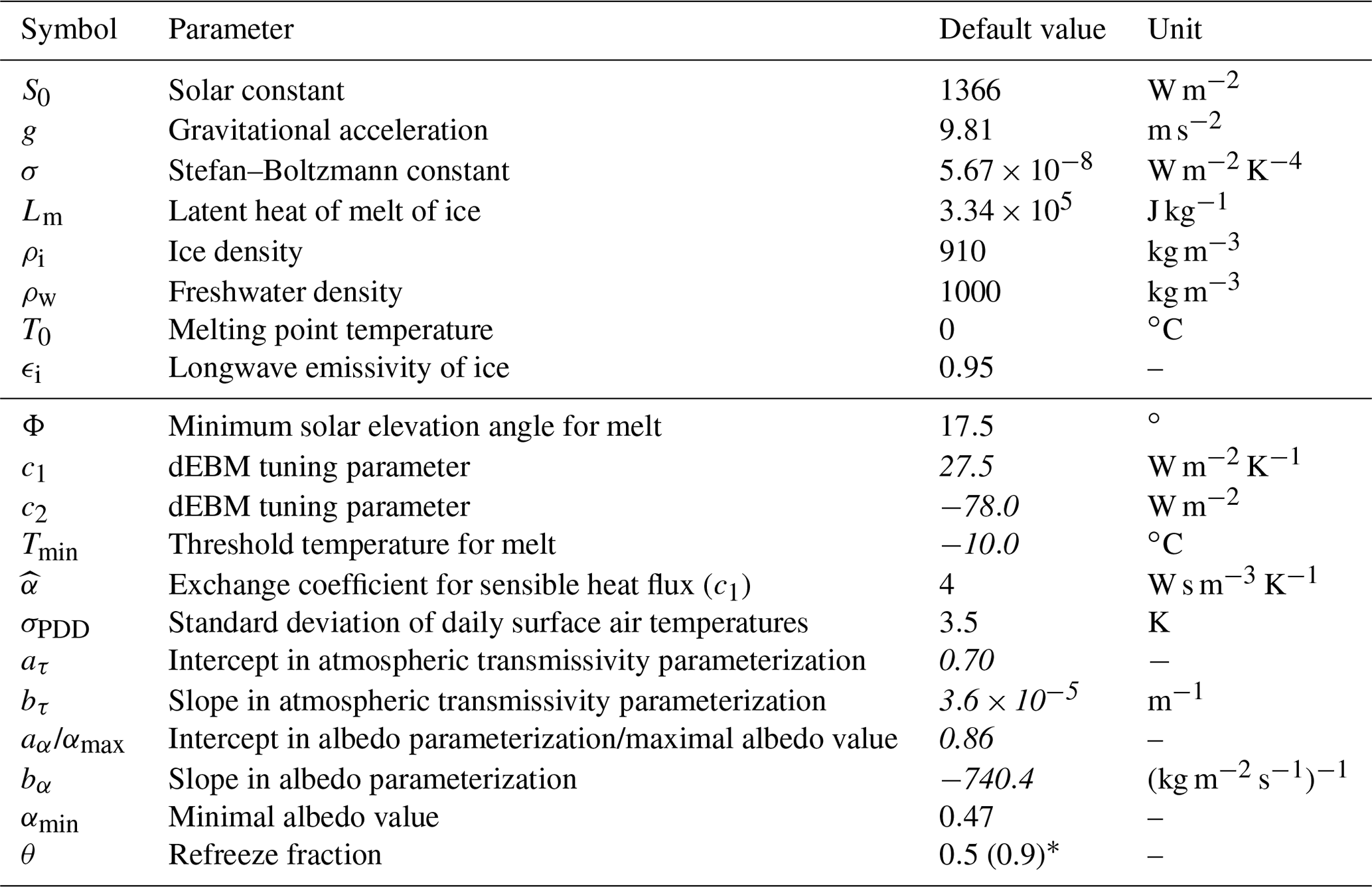
^* The prognostic warming simulations presented here employ θ=0.5 (representative of end-of-century climatic conditions under an SSP5-8.5 warming scenario) as the default. The value given in parentheses (representative of present-day climatic conditions) is used in the historical simulations and for the uncertainty estimation. More details are in the text.

3 Experimental design

In the following subsections we provide a summary of how the initial ice-sheet model state used for the experiments is derived (Sect. 3.1) and describe the climate forcing which is applied as a boundary condition in the experiments at the ice surface and at the ice–ocean boundary (Sect. 3.2). In the last part of the section, we describe the future warming scenarios used to drive the prognostic model simulations (Sect. 3.3).

3.1 Initial ice-sheet configuration

The simulations are initialized from a model state of the Antarctic Ice Sheet that is representative of the ice-sheet configuration in the second half of the 20th century. It is based on an equilibrium state that was prepared for ISMIP6, the Ice Sheet Model Intercomparison Project for CMIP6 (Coupled Model Intercomparison Project Phase 6), and is described in more detail in Reese et al. (2020). The initialization procedure comprises two main steps: first, starting from Bedmap2 ice-sheet geometry (Fretwell et al., 2013), a thermal spin-up simulation is run on a coarser (16 km) model grid for 400 000 years under fixed geometry until the ice sheet reaches a thermodynamic equilibrium with present-day climate. Climatic boundary conditions at the upper ice surface are provided by near-surface air temperature and precipitation fields from RACMO2.3p2 (van Wessem et al., 2018), averaged over the period 1986 to 2005, and at the ice–ocean interface by a data compilation from the World Ocean Atlas 2018 pre-release (Locarnini et al., 2019; Zweng et al., 2019), averaged over 1955 to 2017, and Schmidtko et al. (2014), averaged over the period 1975 to 2012 (for more details, see the following section). Second, starting from this thermodynamic equilibrium state, a simulation ensemble spanning various values of critical model parameters related to basal sliding and sub-shelf melt is run on the 8 km model grid for another 22 000 years under the same climatic boundary conditions with fully evolving physics until the ice sheet reaches a state sufficiently close to equilibrium and ice volume changes become negligible. In the course of these simulations, a comprehensive ensemble scoring scheme is applied after 5000 years and again after 12 000 years in order to select the ensemble member which compares best to present-day observations of ice geometry (Fretwell et al., 2013) and velocities (Rignot et al., 2011). During the entire spin-up, the climatic mass balance (net surface accumulation–ablation rate) and ice surface temperature are directly prescribed from RACMO. For more details on the spin-up and the scoring scheme, see Reese et al. (2020).

3.2 Climate forcing

3.2.1 Air temperature and precipitation

At the ice–atmosphere interface, the climatic boundary conditions (near-surface air temperature and precipitation flux) for dEBM-simple are provided from the polar regional atmospheric climate model RACMO2.3p2 (van Wessem et al., 2018) using simulations covering the period 1950 to 2100. Specifically, we use a historical simulation (1950–2015) and a future projection (2015–2100), which both were generated under climate forcing from the CMIP6-type global coupled climate model CESM2 (Community Earth System Model version 2; Danabasoglu et al., 2020). In a recent intercomparison of five different regional climate models for Antarctica (Mottram et al., 2021), RACMO2.3p2 has been shown to be among the best-performing models when comparing against observations (in terms of both surface air temperatures and surface mass balance), and RACMO's simulated mean annual Antarctic-wide integrated surface mass balance matches the ensemble mean most closely among all ensemble members. RACMO2.3p2 has a comparatively high horizontal and vertical resolution; employs upper-air nudging of temperature and wind fields; and includes a rather sophisticated surface scheme that features a multi-layer snow model calculating meltwater production, percolation, refreezing, and runoff and can account for albedo changes as well as horizontal transport of snow. Comparisons with observations have shown that RACMO has a slight ($\sim -\mathrm{0.5}$ K) cold bias at the surface, resulting in a slight negative bias in modeled surface mass balance and melt rates (Jakobs et al., 2020). Comparing RACMO meltwater fluxes with satellite-derived estimates for the period 2000 to 2009 from QuikSCAT (Trusel et al., 2013), van Wessem et al. (2018) also found a good spatiotemporal agreement between both. While the overall performance is good, small differences exist around the margins of the ice sheet. On the Antarctic Peninsula, RACMO predicts more melt in the northern part of Larsen Ice Shelf, whereas melt is underestimated in the southwestern part. The largest underestimation is shown for Wilkins Ice Shelf on the western Antarctic Peninsula. A comparison of present-day (2000–2009 mean) melt rates between RACMO and QuikSCAT-derived estimates is given in Fig. S4.

The temperature and precipitation fields from RACMO are provided to PISM at a monthly time step in order to resolve the annual climatological cycle and are bilinearly interpolated from the 27 km RACMO grid to the 8 km PISM grid. Note that we here treat all monthly input values as piecewise-constant; i.e., both the air temperature and precipitation values from RACMO are assumed to represent the monthly mean that is valid over the entire course of the month, which is in contrast to the default behavior of PISM where air temperature inputs are interpolated between consecutive forcing data points (see Appendix A for more details).

To account for the surface-elevation–melt feedback, local surface air temperatures are further downscaled according to changes in the ice surface elevation, assuming a spatially uniform atmospheric temperature lapse rate of $\mathrm{\Gamma }=-\mathrm{8.2}$ K km⁻¹. The precipitation field is independent of the evolving ice-sheet geometry, meaning that orography–precipitation interactions (such as a local increase in precipitation when a substantial lowering of the ice-sheet surface leads to a lapse-rate-induced warming and thus a higher moisture-holding capacity of the air layers over the ice-sheet surface) are not accounted for. In the historical calibration experiments, the ice-sheet geometry is kept fixed and thus this lapse rate effect does not apply. Hence, while the absence of orography–precipitation interactions has no effect during calibration, this missing effect could have a slightly mitigating effect on ice-sheet surface elevation changes in the future-warming simulations.

3.2.2 Ocean thermohaline forcing

At the ice–ocean boundary layer, we use the Potsdam Ice-shelf Cavity mOdel (PICO; Reese et al., 2018) to simulate ocean-induced melting below the ice shelves. PICO extends the box model approach by Olbers and Hellmer (2010) for use in 3-dimensional ice-sheet models and thus enables the computation of sub-shelf melt rates consistent with the vertical overturning circulation in the ice-shelf cavities under evolving geometric conditions and in a computationally efficient manner. Oceanic inputs for PICO are provided by observed fields of ocean temperature and salinity at the sea floor on the continental shelf, based on a data compilation from the World Ocean Atlas 2018 pre-release (Locarnini et al., 2019; Zweng et al., 2019), averaged over 1955 to 2017, and Schmidtko et al. (2014), averaged over the period 1975 to 2012. The specifics of the data compilation are described in more detail in Reese et al. (2020). PICO's two main parameters relate to the strength of the overturning circulation and the vertical heat exchange across the ice-shelf–ocean boundary layer and have values of C=1 Sv m³ kg⁻¹ and ${\mathit{\gamma }}_T=\mathrm{3}\times {\mathrm{10}}^{-\mathrm{5}}$ m s⁻¹, respectively, which are tuned to yield melt rates that compare well to present-day observations (Reese et al., 2020).

3.3 Future warming scenarios

To estimate the evolution of Antarctic surface melt under warmer-than-present conditions, PISM-dEBM-simple is forced using a 21st-century warming scenario from RACMO2.3p2 driven by CESM2 and following the Shared Socioeconomic Pathway SSP5-8.5 (Riahi et al., 2017) emission scenario. This scenario represents the highest anthropogenic greenhouse gas emission scenario used by the Intergovernmental Panel on Climate Change (IPCC) and is chosen here to serve as an upper-bound estimate of Antarctic surface melt evolution and resulting ice mass losses under progressing anthropogenic climate change. Note, however, that historical total cumulative CO₂ emissions are in close agreement (within 1 % for the period 2005–2020) with the RCP8.5 emission scenario (the equivalent Representative Concentration Pathway to SSP5-8.5 in terms of radiative forcing) and as of now the RCP8.5 scenario represents the best prediction of mid-century CO₂ concentration levels under current and intended policies (Schwalm et al., 2020). Further, recent comparisons of projected and observed ice-sheet losses from Antarctica have shown that the sea-level equivalent mass losses from the Antarctic Ice Sheet closely track the high end of future sea-level rise projections from the IPCC's Fifth Assessment Report (Slater and Shepherd, 2018; Slater et al., 2020).

To explore the committed impacts of elevated surface melt on the dynamics of the Antarctic Ice Sheet and to estimate the influence the surface-elevation–melt feedback has on the ice sheet, the SSP5-8.5 simulations are extended beyond the end of the available RACMO climate forcing after the year 2100 assuming a steady late-21st-century climate with no further trend. To this aim, the model is forced from 2100 onwards until the year 5000 with a periodic (1-year) monthly atmospheric climatology which is derived from multi-year monthly averages of the decade 2090–2100. This climatic forcing is then kept unchanged throughout the remainder of the simulations irrespective of ice topography changes, whereas the surface air temperature is still allowed to adapt to changes in the ice surface elevation via the lapse rate effect. By the end of these simulations, the ice sheet can be expected to be sufficiently close to equilibrium with the climatic boundary conditions.

Because the main focus of this paper is on the ice sheet's dynamic behavior and response due to changes in the climatic conditions at the ice surface, the forcing at the ice–ocean boundary is fixed throughout the entire simulations. These results thus do not represent realistic projections of the future evolution of the ice sheet. Instead, they likely underestimate total mass loss owing to the disregard of mass losses from increased sub-shelf melting.

4 Model parameter calibration

In a first step, the three main model tuning parameters of dEBM-simple, namely the uncertain constant coefficients c₁ and c₂ from Eq. (6) and the threshold temperature T_min below which no melt should occur (Krebs-Kanzow et al., 2018), are constrained by calibrating the scheme to correctly reproduce historical and present-day spatial and temporal Antarctic melt patterns. For this purpose, an ensemble of fixed-geometry historical simulations is run with PISM-dEBM-simple under monthly 1950–2015 atmospheric boundary conditions from RACMO (see Sect. 3.2.1), spanning all possible parameter combinations of c₁, c₂, and T_min, using a physically motivated best-guess, a minimum, and a maximum plausible value for each of the parameters (in total 3³ realizations).

The optimal parameter set of the calibrated scheme is then selected by scoring the ensemble of historical simulations with respect to RACMO output, taking into account the whole historical period (1950–2015) but also with a specific focus on the scheme's ability to reproduce present-day melt patterns. As a performance score over the historical period we compute the product of the temporal root-mean-square error of yearly total surface melt and the spatial root-mean-square error of surface melt rates averaged over the melting season (DJF). The performance score for the present day is computed from the product of the slope and the Pearson correlation coefficient (R value) of a linear regression fit of 2005–2015 mean summer melt rates computed by dEBM-simple with respect to RACMO. The final score of an ensemble member is then computed as the product of the two normalized individual scores.

The parameter c₁ represents the sensitivity of the melt equation (Eq. 6) to the temperature difference between the melting surface and near-surface air. As in Krebs-Kanzow et al. (2018), we define c₁=3.5 W m⁻² K${}^{-\mathrm{1}}+\widehat{\mathit{\alpha }}u$, accounting for contributions from temperature-dependent longwave radiation and turbulent sensible heat flux, with the latter being linked to surface wind speed u via an exchange coefficient $\widehat{\mathit{\alpha }}$. We here choose $\widehat{\mathit{\alpha }}=\mathrm{4}$ W s m⁻³ K⁻¹ in accordance with estimates at low altitudes by Braithwaite (2009). Given a RACMO-simulated 1950 to 2015 mean summer wind speed at 10 m above ground of 5.3±1.7 m s⁻¹ over the lower (< 2000 m) parts of the ice sheet (Fig. S5), the minimum plausible, best-guess, and maximum plausible values of c₁ are set to {25.5, 27.5, 29.5} W m⁻² K⁻¹, respectively, which corresponds to wind speeds of {5.5, 6.0, 6.5} m s⁻¹. Instead of using the full range of 1 standard deviation around the mean value as estimates for the minimum and maximum plausible values, we thereby restrict the plausible parameter range based on initial sensitivity simulations, such that unrealistically high and low melt rates are discarded.

The melt offset parameter c₂ represents the longwave outgoing radiation. It can in principle be derived from local ice and atmospheric characteristics (Eq. 7 in Krebs-Kanzow et al., 2018); however, using the value given in Krebs-Kanzow et al. (2018) overestimates surface melt over the ice sheet by at least a factor of 2. The plausible range for this parameter is therefore set to {−78, −79, −80} W m⁻². Assuming a longwave emissivity of ice of ϵ_i=0.95, these values suggest an atmospheric emissivity of about 0.74, which is in agreement with clear-sky values found under very dry air conditions on the Antarctic Ice Sheet (Busetto et al., 2013).

The plausible range of the melting threshold temperature T_min, which is used as a background melting condition in the dEBM, is estimated by analyzing historical RACMO surface melt rates with respect to near-surface air temperatures and is set to {−10, −11, −12} ^∘C (Fig. S6).

All other dEBM-simple model parameters (including the albedo and atmospheric transmissivity parameterizations) are set to their respective default values that are given in Table 1. To isolate the computed melt rates from indirect effects of ice dynamics, such as, for example, melt increases caused by lapse-rate-induced surface air temperature changes resulting from dynamic ice-sheet thinning, the ice-sheet geometry is fixed in its present-day configuration. To ensure a consistent comparison, we apply a common ice surface mask for the RACMO and PISM melt fields in all analyses presented here (cf. Hansen et al., 2022).

5 Results

5.1 Model evaluation: historical and present-day melt rates

To evaluate the performance of the calibrated surface melt scheme, we here compare the evolution of Antarctic surface melt over the historical period and for the present-day state as modeled by PISM-dEBM-simple with respect to outputs from RACMO2.3p2 as well as to observation-based estimates derived from QuikSCAT for the decade 2000 to 2009. For comparative reasons, we also compare dEBM-simple-derived melt rates with melt rates produced using PISM's standard PDD melt scheme. The experimental setup and the calibration procedure are described above in Sect. 4. The Antarctica-calibrated optimal values for the three main dEBM tuning parameters c₁, c₂, and T_min resulting from the performance scoring of the tuning ensemble are given in Table 1.

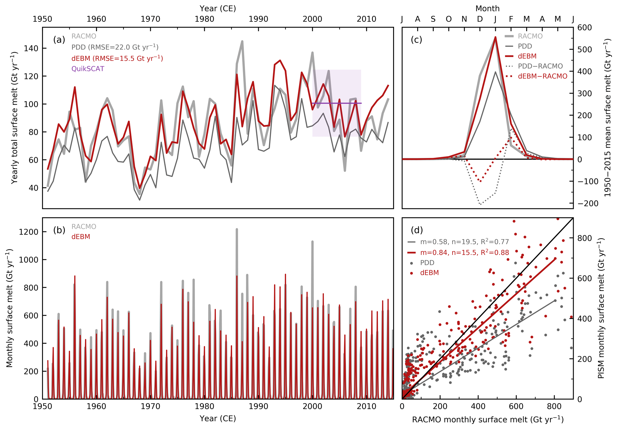
Figure 1 Evolution of total Antarctic surface melt over the historical period computed by dEBM-simple and comparison to RACMO and PDD. (a) Antarctic-wide integrated yearly total surface melt flux (in metric gigatons per year, Gt yr⁻¹) as calculated with PISM-dEBM-simple in the calibrated historical (1950–2015) run (red line). The light-gray line shows the yearly melt flux predicted by RACMO2.3p2 and the thin dark-gray line the melt predicted using PISM with a standard positive degree-day (PDD) melt scheme. For dEBM-simple and PDD, the root-mean-square errors (RMSEs) of yearly total melt fluxes with respect to RACMO are given. Observation-based estimates for the period 2000 to 2009 (mean and standard deviation) based on QuikSCAT data (Trusel et al., 2013) are shown in purple. (b) Monthly surface melt flux (in Gt yr⁻¹) from dEBM-simple (red) and RACMO (light gray). Note that for better comparability monthly values are also given in units of Gt yr⁻¹, i.e., annual flux values. (c) Multi-year monthly averaged annual melt cycle (in Gt yr⁻¹) as simulated by dEBM-simple (solid red line), RACMO (solid light-gray line), and PDD (solid dark-gray line). The dotted lines show the respective differences in melt computed by dEBM-simple and PDD relative to RACMO. (d) Total monthly surface melt fluxes from dEBM-simple and PDD in comparison to RACMO melt fluxes (in Gt yr⁻¹) and linear regression fit of the data (colored solid lines). m and n are the slope and intercept of the regression lines, respectively, and R² the coefficient of determination. The black line marks the identity line.

The evolution of total Antarctic surface melt over the historical period (1950–2015) as computed by the calibrated model setup (Fig. 1) shows that PISM-dEBM-simple is generally able to reproduce the overall magnitudes and temporal patterns of Antarctic surface melt modeled by RACMO2.3p2 for both yearly and monthly² cumulative melt volume fluxes (Fig. 1a–b). Overall interannual variability and trends in the yearly total surface melt flux are captured by the model and track the historical evolution of surface melt diagnosed by RACMO (Fig. 1a). In particular, for the period 2000 to 2009, annual total surface melt volumes fall within the observed QuikSCAT range of 101±24 Gt yr⁻¹ (mean and standard deviation). Considerable deviations in yearly total melt fluxes between dEBM-simple and RACMO output only occur for some extreme melt years and are caused mainly by the treatments of albedo and the incoming surface radiation budget in dEBM-simple, which are unable to reproduce the variability of a more complex climate model like RACMO. The temporal root-mean-square error of the annual total surface melt flux computed by dEBM-simple with respect to RACMO is 15.5 Gt yr⁻¹ and thus approximately 30 % less than the error produced by the PDD scheme (22.0 Gt yr⁻¹; based on default PISM parameter choices).

The multi-year (1950–2015) average seasonal cycle of monthly surface melt fluxes (Fig. 1c) reveals that dEBM-simple captures the peak of the annual melting season as given by RACMO well, with virtually zero difference between both models in January when melt is most intense. However, in comparison to RACMO, dEBM-simple commonly underestimates melting during the first half of the melting season by up to about 100 Gt yr⁻¹ and overestimates melting during the months following the annual melt peak in January by a similar amount. These deviations could be related to the monthly time step of the climate inputs, which hampers the scheme from accurately reproducing the onset and end of the annual melt season, as well to missing processes like, for example, non-radiative heat fluxes such as turbulent latent heat fluxes or conductive subsurface heat fluxes are not accounted for. The same bias occurs for the PDD melt as well; however, it is even more pronounced. In the latter case, the deviations are in part amplified by the treatment of the monthly mean air temperature inputs, where the approach taken here using piecewise-constant temperatures over every full month (see Sect. 3.2.1) leads to slightly colder temperatures from mid-winter (∼ July/August) to the peak of the melting season in January and slightly warmer temperatures during the rest of the year, as compared to the default interpolation approach (for more detail, see Appendix A). Note that integrated over the full year these deviations are mostly canceled out for dEBM-simple, whereas PDD maintains a bias towards lower melt rates.

Comparing monthly Antarctic-wide integrated surface melt rates from dEBM-simple and the PDD scheme with monthly melt rates diagnosed from RACMO yields a better linear regression fit for dEBM-simple (coefficient of determination R²=0.88) than for the PDD scheme (R²=0.77) (Fig. 1d). Both parameterizations show increasing errors with intensifying melt rates, with a positive bias in the lower-melt-rate to medium-melt-rate regime (⪅ 200 Gt yr⁻¹; mainly February melt rates) and a negative bias for the higher-melt-rate regime (⪆ 200 Gt yr⁻¹; mainly December melt rates); however, the error is significantly smaller for dEBM-simple (slope of regression line m=0.84, as compared to PDD with m=0.58). A comparison of annual total Antarctic surface melt rates for all simulations of the dEBM-simple tuning ensemble with respect to RACMO is given in Fig. S7, and a Taylor diagram summarizing the performance of the individual ensemble members is shown in Fig. S8.

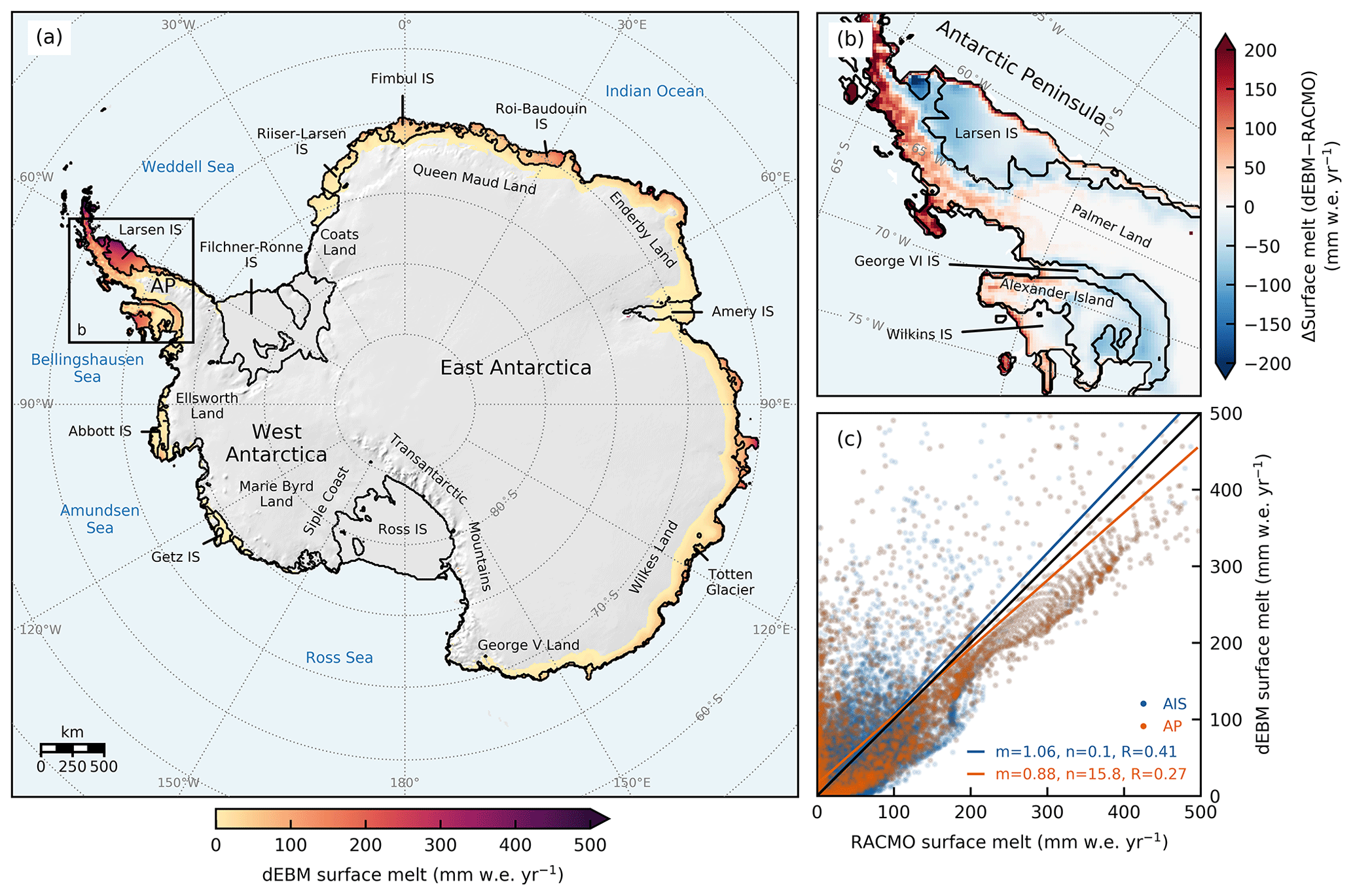
Figure 2 Present-day Antarctic surface melt rates computed by dEBM-simple and comparison to RACMO. (a) Map of mean 2005–2015 Antarctic surface melt rates (in millimeters water equivalent per year, mm w.e. yr⁻¹, as calculated with PISM-dEBM-simple in the calibrated historical run. Areas with melt rates below numerical significance (< 0.001 mm w.e. yr⁻¹) are masked. AP, Antarctic Peninsula; IS, ice shelf. (b) Absolute difference of dEBM-simple minus RACMO-computed surface melt rates (in mm w.e. yr⁻¹), averaged over the same period, shown for a zoomed-in section of the Antarctic Peninsula, the region with the highest average melt rates, indicated by the black square in panel (a). (c) Scatterplot of dEBM-simple versus RACMO-computed surface melt rates (in mm w.e. yr⁻¹) and linear regression fits of the data (colored solid lines). Blue data points correspond to the whole Antarctic Ice Sheet (AIS) and orange data points to the zoomed-in section of the Antarctic Peninsula (AP) shown in panel (b). m and n are the slope and intercept of the regression lines, respectively, and R is the Pearson correlation coefficient. The black line marks the identity line.

The spatial distribution of calibrated present-day (2005–2015 mean) surface melt rates simulated with PISM-dEBM-simple in the historical calibration run as well as a comparison to the respective melt patterns diagnosed from RACMO is shown in Fig. 2. Over the vast majority of the Antarctic Ice Sheet's interior surface, melt is zero or negligible under present-day conditions, while significant surface melt is restricted to a narrow band of low-elevation coastal zones and to the shelves along the margins of the ice sheet north of about 75^∘ S (Fig. 2a). In these areas, spanning nearly the entire coastline of East Antarctica as well as portions of the coast of West Antarctica bordering the Amundsen and Bellingshausen seas, surface melt rates reach values of up to a few hundreds of millimeters water equivalent per year (mm w.e. yr⁻¹); the most intense surface melt at present occurs in the Antarctic Peninsula region with maximum average melt rates exceeding about 400 mm w.e. yr⁻¹ at the northern margin of the Larsen Ice Shelf and 1000 mm w.e. yr⁻¹ towards the northernmost tip of the peninsula.

Comparing the present-day average surface melt patterns predicted by PISM-dEBM-simple with RACMO2.3p2 in general yields a considerable agreement between the two (Fig. 2b–c). While overall dEBM-simple is able to reproduce the localization of melt areas as well as the wide range in surface melt intensities predicted by RACMO, the scheme seems to generally slightly underestimate melt rates in higher-intensity melt regions (i.e., mostly low-elevation ice shelves) and slightly overestimate melt rates in lower-intensity melt regions (e.g., grounded-ice-sheet margins of higher elevations, especially on the Antarctic Peninsula and along the coasts of Wilkes Land and Enderby Land in East Antarctica). The slope of the linear regression fit of grid-point-wise average present-day melt rates from dEBM-simple compared to RACMO is 1.06 (Pearson correlation coefficient R=0.41) for the entire Antarctic Ice Sheet and 0.88 (R=0.27) for the Antarctic Peninsula region (marked by the black square in Fig. 2a), the region with the highest average melt rates. When considering the entire historical period, the values are very similar (m=1.07 and R=0.38 for the whole ice sheet, m=0.92 and R=0.25 for the Antarctic Peninsula; Fig. S9).

The distribution of present-day average surface melt rates modeled with PISM using a standard PDD scheme reveals a substantial overestimation of the average melt area over which significant melt occurs, stretching hundreds of kilometers inland almost along the entire coastline of the continent (Fig. S10). The corresponding linear regression fits for the PDD scheme over the historical period yield slopes of 0.86 (R=0.88) for the entire Antarctic Ice Sheet and 0.73 (R=0.89) for the Antarctic Peninsula region (Fig. S11), indicating that the bias in PDD-modeled melt rate estimates with respect to RACMO is at least 2 times that of dEBM-simple.

A comparison of the spatial melt patterns predicted by PISM-dEBM-simple with the satellite-based melt estimates from QuikSCAT for the decade 2000 to 2009 shows that most of the discrepancies with respect to the observations are indeed “inherited” from RACMO (Fig. S4), which is not surprising given that the scheme is specifically tuned to replicate the RACMO melt patterns (Fig. S12). Melting on the western Antarctic Peninsula on Wilkins and George VI ice shelves and on the southwestern Larsen Ice Shelf and eastern Amery Ice Shelf is also generally underestimated by dEBM-simple. The most notable differences with respect to RACMO are that the overall negative bias in surface melt rates is even more pronounced and the overall spread is higher (for the whole ice sheet, the slope and correlation coefficient of the regression fits for dEBM-simple and RACMO are m=0.70 and R=0.27 and m=0.77 and R=0.74, respectively). Notably, while the overestimation by dEBM-simple of low-intensity melt in the higher-elevation Antarctic Peninsula is not seen in RACMO, the scheme shows a better match for the ice shelves of Queen Maud Land, East Antarctica.

5.2 Projected 21st-century surface melt evolution under SSP5-8.5 warming

The calibrated PISM-dEBM-simple model is now used to run prognostic simulations in order to explore the evolution of Antarctic surface melt in the 21st century and its impact on the surface mass balance of the ice sheet under warmer-than-present atmospheric conditions. The atmospheric boundary forcing for the melt scheme is hereby given by CESM2-driven RACMO2.3p2 using an SSP5-8.5 warming scenario. More details regarding the scenario used are given in Sect. 3.3; the experimental setup is described in Sect. 3.2. In contrast to the model calibration runs presented in Sect. 4, the geometry and dynamics of the ice sheet are now allowed to evolve freely; i.e., the surface-elevation–melt feedback is now accounted for in addition to the melt–albedo feedback. Note that in all following simulations the refreezing of surface meltwater is calculated assuming a refreeze fraction of θ=50 %. The effect of this parameter choice on the committed (long-term) evolution of the surface mass balance as well as the related uncertainty in resulting ice-sheet elevation changes is discussed below in Sect. 5.5.

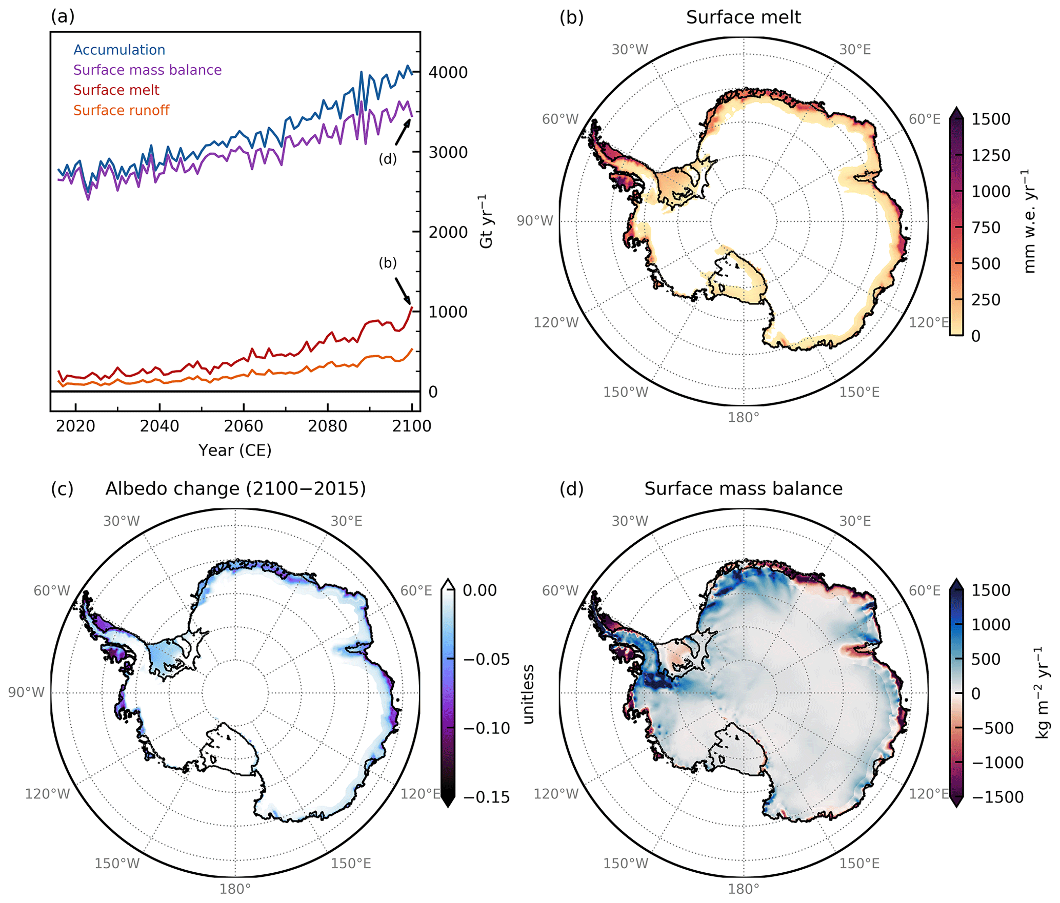
Figure 3 Evolution of Antarctic surface conditions over the 21st century as predicted by dEBM-simple following the SSP5-8.5 scenario. (a) Annual Antarctic-wide integrated surface mass balance components (in Gt yr⁻¹) diagnosed by dEBM-simple using atmospheric boundary forcing from RACMO and assuming an SSP5-8.5 warming scenario. Note that for surface runoff, positive values denote mass losses. (b–d) Annual mean dEBM-simple surface melt (in mm w.e. yr⁻¹), surface albedo change relative to the present day (unitless), and local climatic surface mass balance (in kg m⁻² yr⁻¹; note that 1 kg m${}^{-\mathrm{2}}=\mathrm{1}$ mm w.e.) in 2100.

Despite increasing trends in integrated surface melt and meltwater runoff over the course of the simulation, net mass losses from the ice-sheet surface are overcompensated for by the increase in accumulation (snowfall), resulting in a 30 % increase in net surface mass balance rates by the end of the century compared to the present day, with an average rate of increase of more than 90 Gt yr⁻¹ per decade (Fig. 3a). However, while the surface mass balance of the Antarctic Ice Sheet at present is almost entirely determined by the amount of snowfall and surface meltwater runoff is negligible (∼ 3 % of the annual accumulation rates in terms of absolute magnitude when assuming a refreeze fraction of θ=0.5 and < 1 % when assuming θ=0.9), the abating impact of meltwater runoff on the surface mass balance grows to > 10 % by the end of the century. Antarctic-wide cumulative surface melt volume and meltwater runoff both increase nearly 8-fold from about 96 and 48 Gt yr⁻¹, respectively, at present (2005–2015 mean) to about 860 and 430 Gt yr⁻¹, respectively, by the end of the century (2090–2100 mean) (Table 2).

Table 2 Comparison of Antarctic-wide integrated surface mass balance components and respective standard deviations (in Gt yr⁻¹) as simulated by PISM-dEBM-simple in the calibrated reference configuration, by PISM using a standard PDD scheme, and by the regional climate model RACMO2.3p2. In the case of PISM, the surface mass balance (SMB) is given by the difference between accumulation and runoff. Present-day melt rates are also compared to observation-based estimates from QuikSCAT (Trusel et al., 2013) for the period 2000 to 2009. For the end-of-century surface conditions, melt rates from the Trusel et al. (2015) (T15) RCP8.5 global climate model (GCM) ensemble are also given for comparison.

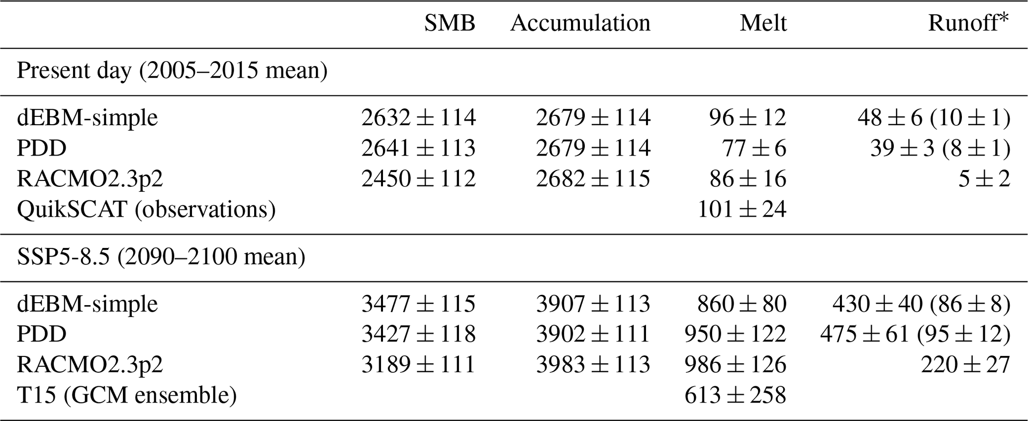
^* Note that for PISM-derived runoff values, the first value assumes a constant refreezing fraction of θ=0.5 (representative of end-of-century climatic conditions under an SSP5-8.5 warming scenario; here used as the default) and the value in parentheses a refreeze fraction of θ=0.9 (representative of present-day climatic conditions). More details are in the text.

Compared to the present day (Fig. 2a), the ice-sheet areas experiencing non-negligible surface melt in 2100 extend to higher surface elevations (up to almost 2500 m, compared to about 1500 m at present; see Fig. S13) and higher latitudes, with some melt on the order of several centimeters per year occurring even south of 85^∘ S, marking the southernmost tip of a broad melt swath stretching across the ice front and western margin of Ross Ice Shelf alongside the Transantarctic Mountains (Fig. 3b). In 2100, significant melt (> 10 mm w.e. yr⁻¹) is found on almost all ice shelves around the coast of Antarctica, including Filchner–Ronne Ice Shelf, all shelves along Queen Maud Land, the Amery Ice Shelf, shelves along Wilkes Land, and all West Antarctic ice shelves bordering the Amundsen and Bellingshausen seas, as well as the entirety of the Antarctic Peninsula below about 2000 m surface elevation, with the only exception of some of the inner parts of Filchner and Ross ice shelves. The greatest increase in mean annual surface melt (> 2000 mm w.e. yr⁻¹) by the year 2100 is found around the northern tip and along the western coast of the Antarctic Peninsula, including Alexander Island. A larger version of Fig. 3b, showing the end-of-the-century surface melt pattern average over the years 2090 to 2100, can be found in the Supplement (Fig. S14).

Through the melt–albedo feedback (Eq. 8), the surface albedo decreases in the melt areas along the ice-sheet margins from its initial value (Fig. 3c). In high-intensity melt regions – mostly on the low-lying ice shelves in East Antarctica, the Amundsen Sea embayment sector in West Antarctica, and on the Antarctic Peninsula – albedo values reduce by up to 0.10 from the maximal value α_max=0.86 that is used in the albedo parameterization as a start value for the simulations. Albedo values below about 0.60 (corresponding to open firn or glacier ice) occur only in some scattered and small locations at the Antarctic Peninsula north of the Antarctic Circle (≈ 66^∘ S), which experience high melt rates on the order of 𝒪(1000 mm w.e. yr⁻¹).

By the end of the century, the elevated surface melt shows a substantial influence on the climatic surface mass balance. While at present the annual climatic surface mass balance is positive across the entire ice sheet, meaning the surface gains more mass from snowfall than it loses by meltwater runoff, in 2100 the ablation areas, i.e., regions that experience a negative annual surface mass balance, extend along almost the entire Antarctic coastline as well as onto large parts of the Amery and Ronne ice shelves, where intensifying surface melt outpaces enhanced mass gains from snowfall (Fig. 3d). Negative surface mass balance in the ice sheet's interior can also be found in the swath of enhanced melt along the western margin of Ross Ice Shelf, extending to about 85^∘ S. The rest of the ice sheet's interior still exhibits net-positive climatic surface mass balance rates in 2100. With respect to the present day, the largest positive changes (i.e., net gain in surface mass balance) in 2100 occur at the higher elevations of the Antarctic Peninsula, Ellsworth Land (West Antarctica), and mountainous regions upstream of Fimbul and Roi Baudouin ice shelves in East Antarctica (gains of more than ∼ 700 kg m⁻² yr⁻¹; note that 1 kg m${}^{-\mathrm{2}}=\mathrm{1}$ mm w.e.). The largest negative changes (i.e., net reduction in surface mass balance) occur along the coasts of the Antarctic Peninsula and Enderby Land, East Antarctica (reductions of more than ∼ 3000 kg m⁻² yr⁻¹).

In comparison to RACMO, the reference configuration of PISM-dEBM-simple predicts about 13 % less cumulative surface melt in 2090–2100 (Table 2). This discrepancy may in part result from the underestimation of higher-intensity melt regimes by dEBM-simple with respect to RACMO, which is already visible under present-day conditions in the form of increased negative biases for higher melt rates (see Figs. 1d and 2b–c), that might negatively impact melt rate estimates under the generally enhanced melt conditions in the warmer climate at the end of the century. Due to the peculiar characteristics of Antarctica's spatial surface melt pattern of a few locally confined high-intensity melt hotspots (⪆ 1000 mm w.e. yr⁻¹) and extensive areas of only low-intensity melting with melt rates up to a few orders of magnitude lower, any underestimation (or overestimation) of the melt rates in these hotspots inevitably leads to relatively large differences in the Antarctic-wide integrated estimates. Being mostly restricted to the northernmost parts of the Antarctic Peninsula, these areas, however, play a minor role in the overall dynamical stability of the Antarctic Ice Sheet. The lower- to medium-intensity melt regimes (⪅ 1000 mm w.e. yr⁻¹), responsible for the surface melt over the vast bulk of the ice sheet, still show a reasonable fit between dEBM-simple and RACMO (Fig. S15; see also Sect. 5.4), suggesting that other ablation processes that are not accounted for in the dEBM approach but are included in RACMO might become more relevant under these high-intensity melt regimes. While dEBM-simple could in principle be tuned in a way to show a better fit in the high-intensity melt regime with respect to RACMO, doing so would contravene the very nature of the scheme, which is based on the assumption of continent-wide spatially uniform parameters.

It is perhaps interesting to point out that dEBM-simple also shows a lower temperature sensitivity of melting as compared to the PDD (see Figs. S16 and S17). In the case of the latter, which calculates melt rates solely on the basis of the temperature forcing, the sensitivity of ice melt to air temperatures is given by the degree-day factor f_i, usually assumed to be ∼ 9 mm w.e. (PDD)⁻¹ (Table S1). The temperature-dependent melt of dEBM-simple (second term in Eq. 6) on the other hand scales with ∼ 7 mm w.e. (PDD)⁻¹ (if expressed in the same units). Thus, once the snow cover is gone, the PDD will react more sensitively to temperature changes (cf. Bougamont et al., 2007). However, while PDD parameters are specifically optimized to correctly reproduce present-day melt rates, these parameters might be not valid in significantly different climates (van de Berg et al., 2011; Robinson and Goelzer, 2014).

5.3 Partitioning drivers of surface melt

The dEBM allows us to partition the relative importance of air temperatures and solar insolation as the drivers of ice-sheet surface melt (see Sect. 2.2.2). Where the total surface melt flux is positive (and hence temperatures are above the melt threshold T_min), we can approximate the relative importance of temperature-dependent melt in the total melt flux by computing the ratio of the melt contribution caused by the air temperature to the sum of the contributions caused by air temperature and incoming solar radiation:

$$\begin{array}{}\text{(10)}& {\mathit{\mu }}_{\mathrm{temp}}:={\displaystyle \frac{M_{\mathrm{temp}}}{M_{\mathrm{temp}}+M_{\mathrm{insol}}}}.\end{array}$$

Thereby, the insolation-driven melt contribution, $M_{\mathrm{insol}}\propto (\mathrm{1}-\mathit{\alpha })\mathit{\tau }{\mathrm{SW}}_{\mathrm{\Phi }}$, is given by the first term of Eq. (6) and represents the net uptake of incoming solar shortwave radiation of the surface during the diurnal melt period. The temperature-driven melt contribution, M_temp∝c₁ T_eff, is given by the second term of Eq. (6) and represents the air-temperature-dependent part of the incoming longwave radiation (linear term in Eq. 5 of Krebs-Kanzow et al., 2018) as well as turbulent sensible heat fluxes. Note that due to the (negative) melt offset, M_off∝c₂, which is given by the third term in Eq. (6) and which represents the outgoing longwave radiation flux as well as the air temperature-independent part of the incoming longwave radiation (constant term in Eq. 5 of Krebs-Kanzow et al., 2018), the radiation-driven component of the dEBM would in theory only result in a positive contribution to the total melt flux if the sum $M_{\mathrm{insol}}+M_{\mathrm{off}}>\mathrm{0}$. However, since M_off is mostly constant if the surface is near the melting point (Fig. S18) and is independent of changes in insolation or air temperature and thus independent of the climate scenario, Eq. (10) constitutes a useful approximation for all areas exhibiting a positive total melt flux.

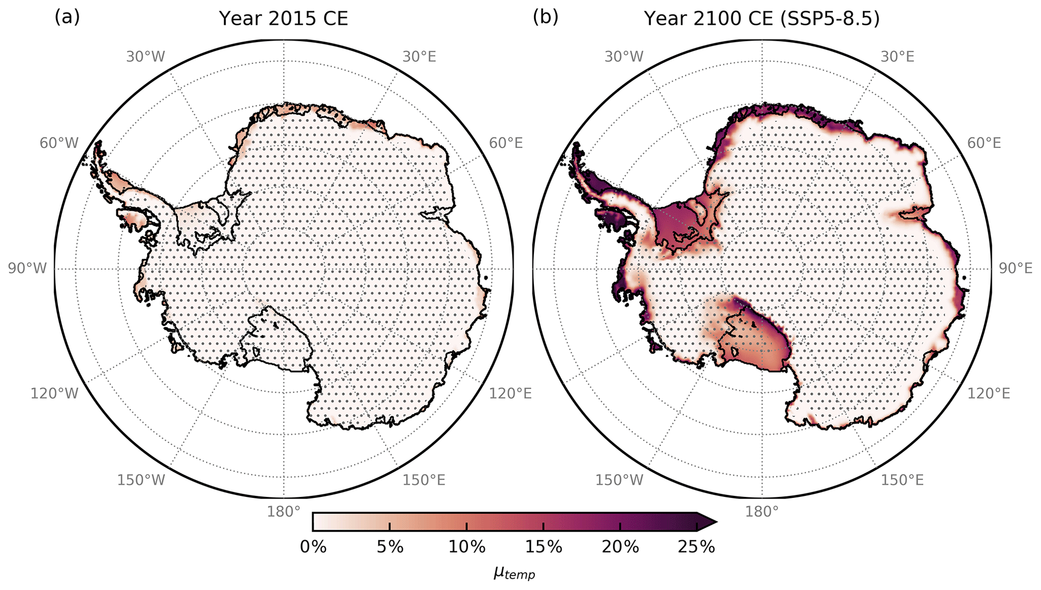
Figure 4 Relative importance of temperature-dependent melt for total surface melt. Ratio of annual average temperature-driven melt to the sum of temperature- and insolation-driven melt contributions ${\mathit{\mu }}_{\mathrm{temp}}=M_{\mathrm{temp}}/(M_{\mathrm{temp}}+M_{\mathrm{insol}})$ (in percent) as an approximation of the relative importance of temperature-dependent melt to total melt, shown for the years 2015 (a) and 2100, assuming an SSP5-8.5 warming scenario (b). Areas where annual average total surface melt is zero are dotted.

The change in the relative importance of temperature-driven vs. insolation-driven melt, μ_temp, from the present day to 2100 derived from the SSP5-8.5 simulations is depicted in Fig. 4. On average, incoming solar shortwave radiation is the dominant driver of ice surface melt over the whole Antarctic Ice Sheet, both under present-day and under warmer end-of-century climate conditions. At present, the annual average relative share of temperature-driven melt μ_temp is comparatively small, ranging between almost zero and about 10 % in the ice-sheet areas that experience non-negligible surface melting, with higher values only occurring in small places at the tip of the Antarctic Peninsula north of about 65^∘ S (Fig. 4a). By the end of the century, both the temperature-driven melt contribution M_temp and the insolation-driven melt contribution M_insol have increased substantially. While the increase in M_temp is due to the overall increasing temperatures, the increase in M_insol results from the overall reduction in surface albedo in areas experiencing substantial surface melt, enhanced by the melt–albedo feedback. In high-intensity melt areas with significantly lower ice albedo values, like, for example, the Larsen or Wilkins ice shelves, M_insol increases by some 20 % to 30 %, while M_temp increases by about 300 % to 400 % and above, more than an order of magnitude more. As a result, the average annual share of temperature-driven melt μ_temp increases to about 15 % to > 25 % in high-intensity melt areas along the ice-sheet margins by the year 2100 (Fig. 4b). Even in 2100, an average annual peak share of temperature-driven melt of more than 40 % is only exceeded in small regions around the tip of the Antarctic Peninsula, where monthly mean temperatures reach as high as a few degrees above the melting point. On the other side, over extensive areas in cold and high-altitude regions along the margin of East Antarctica, surface melting is driven almost entirely by solar insolation, provided that monthly mean air temperatures exceed the threshold temperature $T_{\min }=-\mathrm{10}$ ^∘C below which any melt is suppressed.

5.4 Uncertainty estimation of predicted 21st-century surface melt

The model results presented in the above sections were obtained using a reference set of calibrated dEBM-simple model parameters that provide the best fit to historical and present-day melt rates from RACMO2.3p2. However, the predicted evolution of surface melt rates over this century as diagnosed by dEBM-simple is subject to uncertainties related to poorly confined model parameters. In addition to the three main dEBM-simple tuning parameters (c₁, c₂, T_min; see Sect. 4), the parameterizations of the surface albedo and the atmospheric transmissivity within dEBM-simple each contain two more uncertain parameters (a_α, b_α and a_τ, b_τ; see Sect. 2.2.3 and 2.2.4, respectively).

To check the robustness of the predicted surface melt evolution in the SSP5-8.5 simulations with regard to uncertain model parameter choices, we run an ensemble of model simulations in which we account for deviations of those parameters from their respective default values. The model ensemble consists of 41 simulations sampling various combinations of different parameter values.

For the three main model tuning parameters c₁, c₂, and the threshold temperature for melt T_min, we adopt the same values as were used for the calibration (Sect. 4), which we cross-combine in the ensemble. To estimate the uncertainty from the albedo parameterization, we adopt values for the intercept a_α (which is identical to the maximum albedo α_max) and the slope b_α that are obtained from linear regression fits of 2085–2100 multi-year mean monthly RACMO2.3p2 data averaged over the austral summer months December, January, and February, respectively, following the SSP5-8.5 warming scenario (Fig. S3). The values adopted for the intercept a_α are {0.85, 0.86, 0.87, 0.88} and for the slope b_α are {−1082.0, −740.4, −500.3} (kg m⁻² s⁻¹)⁻¹. Since the intercept and slope of the fits are not independent of each other, we combine the two lower albedo intercepts (0.85 and 0.86) only with less steep slopes (−740.4 and −500.3 (kg m⁻² s⁻¹)⁻¹), the higher albedo intercept (0.87) only with steeper slopes (−1082.0 and −740.4 (kg m⁻² s⁻¹)⁻¹), and the highest intercept (0.88) only with the steepest slope (−1082.0 (kg m⁻² s⁻¹)⁻¹) (see Table 3).

In a similar fashion, we estimate the uncertainty related to the atmospheric transmissivity parameterization by varying the values of the parameters a_τ and b_τ on the basis of linear regression fits of 1950–2015 multi-year mean monthly RACMO2.3p2 data averaged over the months with the highest monthly TOA insolation: November, December, and January, respectively (Fig. S2). The values adopted for the intercept a_τ are {0.68, 0.70, 0.72} and for the slope b_τ are {3.3, 3.6, 3.9} × 10⁻⁵ m⁻¹. Due to limitations in computational capacity we combine the varied parameters from the albedo and transmissivity parameterizations only with the reference set of the main dEBM parameters, instead of cross-combining all possible combinations.

Table 3 Parameter value combinations of intercept a_α and slope b_α of the albedo parameterization of dEBM-simple used in the model sensitivity ensemble. The bold symbol marks the reference parameter combination.

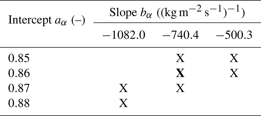
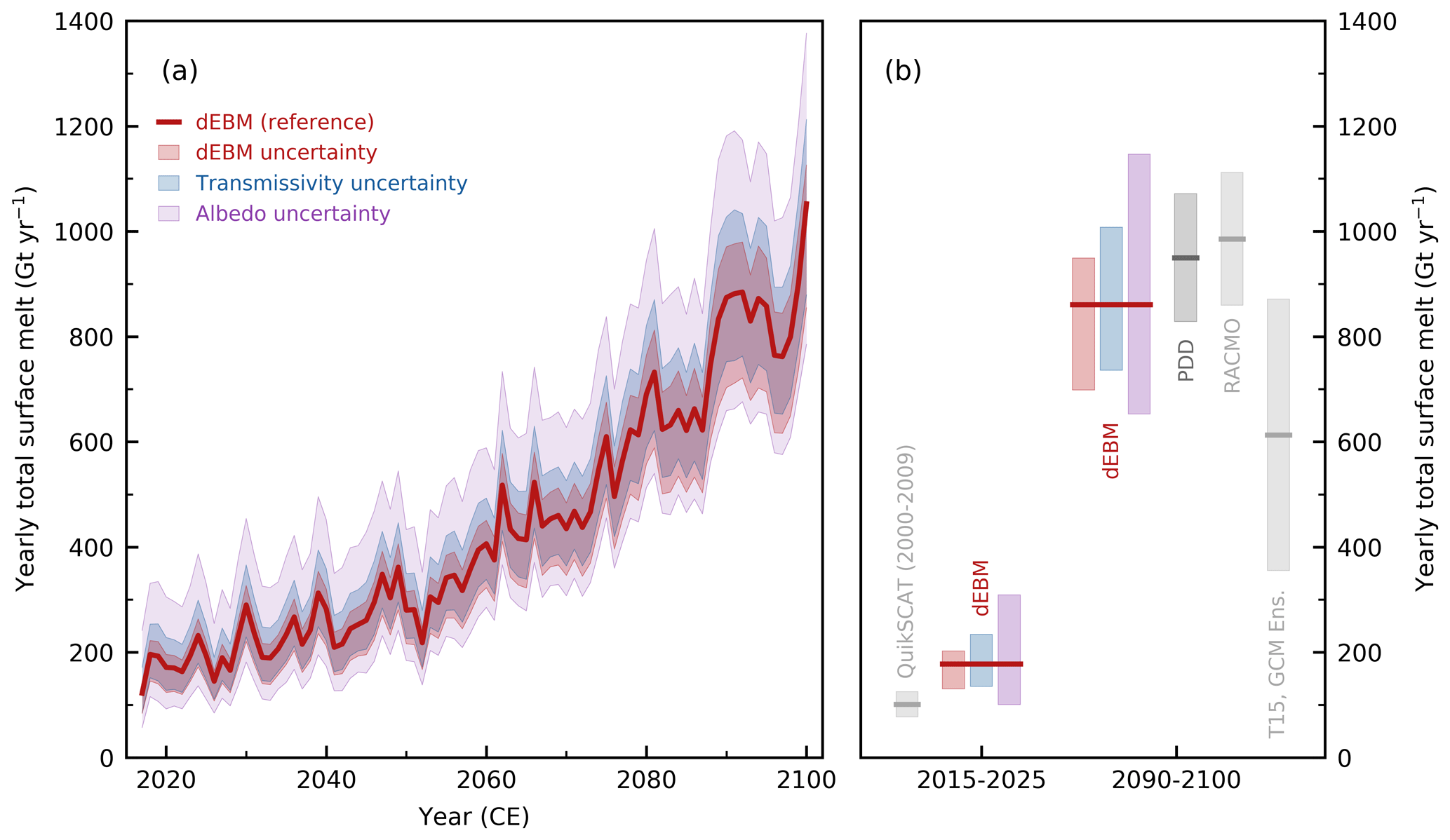
Figure 5 Evolution of total Antarctic surface melt under SSP5-8.5 according to dEBM-simple and related model uncertainty spread. (a) Antarctic-wide integrated annual total surface melt flux (in Gt yr⁻¹) as predicted by PISM-dEBM-simple using the reference parameter configuration under boundary forcing from RACMO2.3p2 and assuming an SSP5-8.5 warming scenario (red line). Red shading shows the model ensemble spread related to uncertainty in the three main dEBM tuning parameters (c₁, c₂, T_min), blue shading the uncertainty spread related to the transmissivity parameterization (a_τ, b_τ), and purple shading the uncertainty spread related to the albedo parameterization (a_α, b_α). (b) Mean annual surface melt (reference model parameters; red lines) and respective uncertainty spreads of the three contributions at indicated decades, as well as comparison to other estimates: observation-based estimates for the period 2000–2009 are based on QuikSCAT data (Trusel et al., 2013). For the period 2090–2100, the dark-gray bar shows the estimate from PISM using a standard PDD scheme and light-gray bars show the respective estimates from RACMO2.3p2 as well as the RCP8.5 GCM ensemble from Trusel et al. (2015) (T15). In the latter three cases, the uncertainty spread is given by the standard deviation.

The maximal uncertainty spread of modeled annual total surface melt resulting from the parameter variations in the model sensitivity ensemble increases over the 21st century from about 200 Gt yr⁻¹ (2015–2025 average) to about 500 Gt yr⁻¹ (2090–2100 average; Fig. 5). The total uncertainty spread is thereby dominated by the uncertainty due to the albedo parameterization, which increases surface melt sensitivity to incoming shortwave radiation via both lower maximal albedo values α_max and stronger albedo sensitivities, i.e., steeper slopes b_α in the albedo parameterization (Eq. 8). The uncertainty spreads related to the main dEBM-simple parameters and the transmissivity parameterization are both only about half of that (⪅ 100 Gt yr⁻¹ in 2015–2025 and ∼ 250 Gt yr⁻¹ in 2090–2100, respectively). The upper end of the total uncertainty spread is dominated by a slightly lower maximal albedo of α_max=0.85 (under otherwise default model parameters) and a steeper slope of $b_{\mathit{\alpha }}=-\mathrm{1082.0}$ (kg m⁻² s⁻¹)⁻¹ in combination with α_max=0.87 (and otherwise default model parameters) towards the end of the century. The lower end of the total uncertainty spread is dominated by the slightly higher maximal albedo values α_max=0.87 and 0.88 (even in combination with steep albedo slopes) until around the middle of the century and slightly higher maximal albedo values α_max=0.87 (in combination with the default albedo slope) as well as default maximal albedo combined with the least steep slope $b_{\mathit{\alpha }}=-\mathrm{500.3}$ (kg m⁻² s⁻¹)⁻¹ thereafter. Variations in the parameters from the transmissivity parameterization (Eq. 7) result in deviations of modeled end-of-century surface melt of up to about ±15 % relative to the reference simulation. The influence of variations in T_min is only minor compared to that of the other parameters.

The maximal uncertainty range of modeled mean annual total surface melt of about 650 to 1150 Gt yr⁻¹ projected for the decade 2090 to 2100 with PISM-dEBM-simple is considerably higher but overlaps in part with the possible range of Antarctic surface melt volumes estimated in an earlier study by Trusel et al. (2015) based on a model ensemble of five selected global climate models from the CMIP5 (Coupled Model Intercomparison Project Phase 5) ensemble under RCP8.5 (about 360 to 870 Gt yr⁻¹ for 2091–2100). The reference configuration of PISM-dEBM-simple predicts ∼ 40 % more melt for that decade than the Trusel et al. (2015) model ensemble (decadal mean values are 860 and 613 Gt yr⁻¹, respectively) while at the same time predicting about 10 % less than RACMO2.3p2 despite overlapping uncertainty ranges (Fig. 5b). The slightly higher value of the PDD model with respect to dEBM-simple can primarily be attributed to the higher temperature sensitivity of that scheme (cf. Bougamont et al., 2007).

5.5 Committed impacts of enhanced surface melting on ice-sheet dynamics

Due to the long response time and large inertia of the Antarctic Ice Sheet, the impact of increased surface melting on the dynamics of the ice sheet has not played out in full by the end of the simulations in 2100. Furthermore, feedback mechanisms that potentially amplify those changes – especially the surface-elevation–melt feedback – operate on longer timescales (∼ several centuries to millennia), leading to a time lag between cause and effect on the order of multiple centuries. To investigate the committed impacts of elevated end-of-century surface melting on the ice-sheet dynamics, we extend the SSP5-8.5 simulations beyond the end of the available RACMO forcing after the year 2100 under fixed end-of-century (2090–2100 monthly mean) climate conditions until the year 5000 (see Sect. 3.3 for further details). By this time, the ice sheet has reached a state close to equilibrium with the atmospheric boundary conditions.

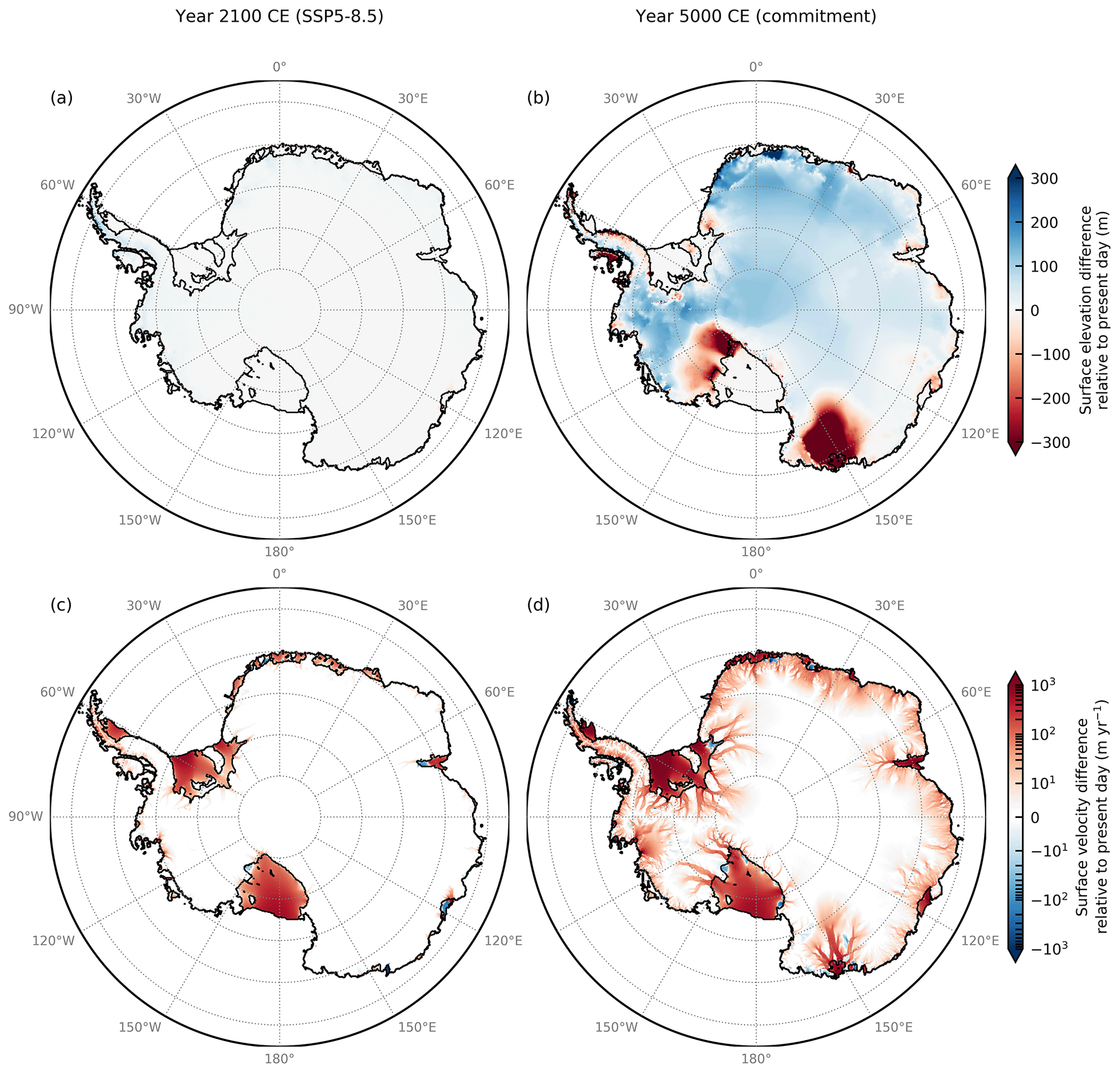
Figure 6 Committed dynamical changes in Antarctica resulting from enhanced surface melting. Difference in ice-sheet surface elevation (in m) as modeled with PISM-dEBM-simple under SSP5-8.5 forcing from RACMO2.3p2 compared to a control simulation run under present-day (1986–2015 mean) conditions (a) in 2100 and (b) under sustained end-of-century (2090–2100 monthly mean) climate conditions in the year 5000. (c–d) Same as panels (a) and (b) but for ice surface velocity (in m yr⁻¹).

The dynamical and topographical changes that the Antarctic Ice Sheet is committed to under the intensified surface melt at the end of the century even without any further warming are strong (Fig. 6). While the ice-sheet surface elevation changes in 2100 compared to 2015 (both positive and negative) range between a few meters in the ice sheet's interior and several tens of meters in regions nearer to the coast, surface elevation changes in the year 5000 have increased by about 1 order of magnitude in both directions (Fig. 6a–b). Regions experiencing positive elevation change (i.e., thickening) caused by enhanced snowfall are, e.g., Queen Maud Land, East Antarctica, and Ellsworth Land, West Antarctica, whereas regions with negative elevation change (i.e., thinning) are, e.g., George V Land, East Antarctica; Marie Byrd Land, West Antarctica; and Alexander Island, Antarctic Peninsula. The strongest reductions in surface elevation are found in catchment basins of glaciers draining the George V coast of the Wilkes Subglacial Basin, East Antarctica, and on Alexander Island (up to about 1000 m of dynamic thinning), as well as on ice streams along the West Antarctic Siple and Gould coasts feeding into Ross Ice Shelf (up to about 500 to 600 m of dynamic thinning).

In particular, the Wilkes Subglacial Basin in East Antarctica has recently raised increasing concern as the ice in this drainage basin rests on deep, inland-sloping bedrock submerged well below sea level, rendering it susceptible to unstable and potentially irreversible marine ice-sheet collapse (Mengel and Levermann, 2014; Sun et al., 2016; Pelle et al., 2021). Long-term model simulations have shown that this catchment basin is particularly sensitive to warmer air temperatures, while being relatively inert with respect to ocean warming alone (Golledge et al., 2017). In contrast, glaciers in the Amundsen Sea embayment region of West Antarctica are much more sensitive to ocean forcing and show only little response to atmospheric warming alone.

Interestingly, these results are fairly robust with regard to changes in modeled meltwater runoff, i.e., the refreeze fraction parameter θ. Assuming a value of θ=0.9, which is more representative of present-day cold conditions, as a kind of conservative upper bound (instead of the default value θ=0.5, which is more representative of warm end-of-century SSP5-8.5 conditions), the overall pattern of surface elevation and velocity changes remains similar (Fig. S19). The slightly higher overall surface mass balance in the θ=0.9 simulation compared to the θ=0.5 simulation generally leads to even more pronounced positive elevation changes (i.e., thickening) over most of the ice sheet, whereas the thinning in the Wilkes Subglacial Basin is even slightly stronger (Fig. S20). Given that even under ∼ 2100 climatic conditions the surface mass balance is largely dominated by accumulation in these regions (Fig. 3d) and ablation is low and confined to narrow bands along the coast (Fig. 3b), the negligible influence of the refreezing parameter θ is not surprising since the thinning of these regions is primarily a consequence of internal ice dynamics rather than a negative surface mass balance. However, gradual initial surface melting due to atmospheric warming appears to act as the trigger for this unstable retreat. For the Wilkes Subglacial Basin in particular, Golledge et al. (2017) have shown that surface melting may be a mechanism by which a coastal “ice plug” (Mengel and Levermann, 2014) that currently prevents irreversible ice discharge from that region could be removed.

The substantial differences between the century- and millennium-scale response of the ice-sheet surface elevation, even in the absence of further warming, also point to the vital role of the surface-elevation–melt feedback: while the initial surface lowering near the coast is caused by intensified surface melt and meltwater runoff, the feedback cycle between surface altitude and melt commits the ice to self-sustained dynamic thinning and inland retreat, independently of the climatic forcing, further amplifying dynamically driven mass losses.

The changes in ice surface velocities associated with these surface elevation changes are illustrated in Fig. 6c–d (and Fig. S19c–d for the θ=0.9 simulation). Apart from a few exceptions, the vast majority of the Antarctic ice shelves already experience a significant speed-up in ice flow in response to surface melt intensification and subsequent thinning by 2100, with further acceleration by the year 5000. This leads to a slight acceleration of upstream ice over most of the ice sheet, which propagates inland for hundreds of kilometers via the tributary glacier systems. In the year 5000, accelerated ice surface flow speeds are found almost over the entire ice sheet, stretching far inland. Note that most of the thinning results from accelerated ice flow and discharge into the ocean, whereas the climatic surface mass balance is often still positive over regions with decreasing surface elevations. Importantly, the observed dynamical thinning and acceleration of the ice sheet happen despite an overall positive surface mass balance.

6 Discussion

The dEBM-simple model calculates ice-sheet surface melt on the basis of the surface energy balance of the daily melt period and simulates insolation- and temperature-driven surface melting from changes in surface albedo and seasonal as well as latitudinal variations in the daily insolation cycle. As such, it is more physically constrained than even simpler empirical temperature-index schemes such as the positive degree-day (PDD) method, which are still widely used in long-term ice-sheet model experiments to compute surface melt rates in centennial- to millennial-scale continental simulations. Furthermore, due to its high computational efficiency, dEBM-simple can be used to replace less confined temperature-index-based surface melt schemes such as the PDD method in ice-sheet model simulations.

The dEBM-simple model only takes monthly mean forcing inputs, yet it implicitly accounts for the diurnal cycle of shortwave radiation and insolation-driven surface melt. By using efficient parameterizations for incoming TOA shortwave radiation, atmospheric transmissivity, and ice surface albedo (Zeitz et al., 2021), the number of required inputs can be kept at a minimum. In addition to monthly mean surface air temperature fields, the implementation of dEBM-simple in PISM only requires monthly mean precipitation fields as inputs in order to close the climatic surface mass balance in standalone ice-sheet model simulation runs. Thereby, precipitation is passed unaltered through the scheme, whereas the respective shares of snowfall and rain are determined based on local air temperatures.³

Overall, dEBM-simple is capable of reproducing Antarctic historical and present-day surface melt rates with regard to spatial as well as temporal patterns considerably well, including interannual variability and trends. Without compromising on computational efficiency, the scheme performs better than the empirical PDD method in various respects under the same atmospheric climate boundary conditions. Compared to a standard PDD configuration, dEBM-simple shows smaller errors in simulated total monthly and annual surface melt volume over the historical period, a better spatial representation of present-day and end-of-century melt patterns and melt area extent over the entire ice sheet as well as over the Antarctic Peninsula in particular, and a better representation of the average yearly melt cycle.

In the following, we address some model limitations and discuss their influence on the presented findings. Being a simple model, dEBM-simple does not resolve the spatial and temporal patterns of historic and present-day surface melt over the Antarctic Ice Sheet in full detail. Nevertheless, with well-calibrated model parameters the scheme is able to reproduce historic and present-day melt rates considerably well, justifying its application for future ice-sheet projections.

In comparison to the more complex regional climate model RACMO2.3p2, dEBM-simple in general slightly underestimates melt rates in high-intensity melt regions and during the first half of the melting season (mainly December), while slightly overestimating melt rates in low-intensity melt regions and during the months following the annual melt peak (mainly February). This bias is likely related to the use of spatially uniform and temporally invariant parameters – first and foremost the two dEBM parameters c₁ and c₂ which depend on the atmospheric emissivity and can not represent the spatial and temporal variability due to changing cloud cover – as well as phenomenologically based linear relationships to parameterize the melt–albedo feedback and the atmospheric transmissivity.

In particular, the assumption of a first-order linear dependence of ice albedo on surface melt rates is only a rough representation of the numerous factors and processes that influence ice and snow albedo, such as snow grain size, impurities (dust/soot content, debris cover), surface water aggregation and supraglacial melt ponds, the solar zenith angle, and cloud cover (Gardner and Sharp, 2010). Especially the changes in snow grain sizes, e.g., due to snow aging, are an important factor that is neglected in the model but plays a major role for the albedo. While snow aging generally leads to a reduction in albedo and its neglect should therefore in principle lead to an underestimation of melt rates at the end of the melt season, there are important processes that act in the opposite direction: a major caveat of the scheme is that it neglects the influence of changes in snow cover thickness that could mitigate the melt-induced reduction in albedo after heavy-snowfall events or inhibit the melt–albedo feedback (Picard et al., 2012; Jakobs et al., 2021). However, on the long timescales considered here individual snowfall events are likely to only play a minor role as compared to the mean surface conditions. Further, while we here focus on the long-term evolution of the ice sheet and thus deliberately chose to employ the albedo parameterization, we should point out that this shortcoming could be easily resolved by reading in albedo fields from more sophisticated process-based snowpack models, provided that reliable data are available for the time period of interest.

Similarly to the albedo approach, the parameterization of the atmospheric transmissivity is based on the assumption of time-invariant and spatially uniform parameters and thus does not account for spatial or temporal variability in cloud patterns or orographic effects. While the polar atmosphere over Antarctica is currently in general clean and dry and reasonably thin with only low cloud cover over the ice sheet, the assumption of constant parameters poses quite a strong constraint under future warmer conditions (see, e.g., Kittel et al., 2022), for which the “full” dEBM scheme (Krebs-Kanzow et al., 2021), which features a variable cloud cover, might be more appropriate.

Using only one set of constant model parameters that are applied uniformly over the entire model domain in time and space (in our case, e.g., c₁, c₂, σ_PDD, Φ) might further cause systematic biases in comparison to a process-based model such as RACMO by ignoring topography-dependent regional patterns and seasonal variability. As an example, the standard deviation of daily temperatures σ_PDD has been shown to exhibit high spatial and seasonal variability that might cause significant discrepancies in surface mass balance computations (e.g., Seguinot, 2013; Rogozhina and Rau, 2014). Similarly, the value for the minimum solar elevation angle Φ that is used here is adopted from Krebs-Kanzow et al. (2018) and roughly estimated based on typical present-day summer insolation and snow albedo values, an assumption that might not be valid in future warmer climates and that is improved in the “full” dEBM scheme (Krebs-Kanzow et al., 2021) by computing Φ explicitly based on local atmospheric conditions; for a more detailed discussion and sensitivity analysis of this parameter, see Krebs-Kanzow et al. (2018). The dEBM-simple parameters c₁ and T_min, governing the temperature dependency of melt, in general favor more intense melt with higher absolute values, whereas c₂, related to longwave outgoing radiation, has a mitigating effect for higher absolute values. However, the influence of these main dEBM-simple parameters is less than that of the albedo and transmissivity parameterizations.

The spatiotemporally constant refreezing factor θ, which regulates how much meltwater runs off the ice sheet and thus directly affects surface mass losses and changes in ice-sheet elevation, adds another source of uncertainty that is particularly relevant to the long-term dynamical evolution of the ice sheet as it acts as a trigger for the surface-elevation–melt feedback. As refreezing is highly variable both spatially and temporally (van Wessem et al., 2018; Fig. S1), the assumption of constant, uniform values provides only a coarse representation of a complex process that could be further constrained by applying a refreezing parameterization that is either temperature-dependent or based on negative net surface energy fluxes, as done, for example, in Krebs-Kanzow et al. (2021) or Krapp et al. (2017). Note, however, that the wide range tested for this parameter (between 50 % and 90 %) has only a negligible impact on the presented results, in particular, but not only, for the committed dynamical ice-sheet evolution. Importantly, while even under the warmer end-of-century climate conditions the surface mass balance over most of the ice sheet is largely dominated by snowfall and ablation is low, enhanced surface melt due to atmospheric warming may act as a trigger for unstable dynamically driven retreat in marine ice-sheet regions that are susceptible to instability mechanisms.

Being a simple model, dEBM-simple is unable to capture melt associated with orographic features around the edges of the ice sheet, such as foehn winds or warm katabatic winds, which can enhance melting near the grounding line (Datta et al., 2019; Lenaerts et al., 2019). To adequately capture the effects of orography–precipitation interactions, for example, fully coupled ice–atmosphere models are needed. However, smaller-scale melt characteristics or single extreme melt events are likely to be of less importance on the long timescales (i.e., glacial-cycle timescales in both the deep past and the deep future) that are the primary focus of the present approach, where the melt “climate” is more important than the melt “weather” (van den Broeke et al., 2023).

Finally, surface ablation contributions resulting from sublimation and evaporation have so far not been considered in the present model setup. While evaporation might likely be negligible in comparison to the other ablation processes at present (Lenaerts et al., 2019), it might become more important in the future, especially under strong warming. Sublimation under high-wind and dry atmospheric conditions as found, for example, in the escarpment zones, on low-lying blue ice areas and ice shelves, or even in parts of the ice-sheet interior where strong katabatic winds prevail (Lenaerts et al., 2019; Das et al., 2013) can also be a considerable factor in the surface mass balance that could be improved in future work.

7 Summary and conclusions

In this work we have applied the newly developed intermediate-complexity surface melt scheme dEBM-simple in an Antarctic Ice Sheet configuration to assess the possible range of future surface melt trajectories in Antarctica under a strong-global-warming scenario as well as their impact on ice-sheet dynamics. The dEBM-simple model is a slightly modified version of the “simple” diurnal Energy Balance Model (Krebs-Kanzow et al., 2018) that has been adopted by Zeitz et al. (2021) as a fully fledged surface mass balance module in the Parallel Ice Sheet Model (PISM-dEBM-simple) for application on the Greenland Ice Sheet. The implementation of dEBM-simple in PISM including the adopted modifications with respect to the model formulation given in Krebs-Kanzow et al. (2018) as well as its calibration and validation for the Greenland Ice Sheet is described in more detail in Zeitz et al. (2021).

The dEBM-simple model is a fast and computationally inexpensive model and is specifically developed for the use in long-term (millennial-scale) standalone prognostic ice-sheet model simulations or model ensembles in applications over glacial-cycle timescales in both the deep past and the deep future. The physically based model improves upon conventional and empirically based temperature-index schemes (such as the positive degree-day, PDD) by accounting for the daily energy cycle at the ice surface on the basis of orbital configuration, latitude, and season, despite requiring only monthly inputs of 2D near-surface air temperatures as boundary forcing. Due to simple but efficient parameterizations for incoming shortwave solar radiation and ice albedo changes, it explicitly includes insolation-driven melt and is able to account for the positive melt–albedo feedback. Thus, it fills the gap between sophisticated regional climate models coupled with multi-layer snowpack models that feature physics-based process detail but come at the cost of high computational expenses and empirical temperature-index schemes that are fast enough for glacial-cycle timescales but do not account for small-scale processes at the ice–atmosphere interface, potentially neglecting important feedbacks.

In this work, we have calibrated PISM-dEBM-simple for Antarctica using a model ensemble and historical (1950–2015) atmospheric forcing from the polar regional atmospheric climate model RACMO2.3p2. We have shown that the calibrated model is able to reproduce historical Antarctic melt rates from RACMO and satellite-derived estimates in terms of interannual variability, trend, and spatial patterns considerably well, which justifies its application in future ice-sheet projections. In idealized 21st-century (2015–2100) warming simulations under a RACMO-CESM2-forced SSP5-8.5 atmospheric warming scenario, we have used dEBM-simple in a second model ensemble to explore the range of possible future surface melt trajectories, specifically focusing on the model's sensitivity to parameter choices. By partitioning temperature- and insolation-driven surface melt, the dEBM-simple approach is able to reveal a significant increase in the relative share of temperature-induced melting in total surface melt over the course of the century. Finally, we have investigated the committed effects of enhanced surface melting on the dynamics of the Antarctic Ice Sheet by extending the SSP5-8.5 simulations beyond 2100 under fixed end-of-century atmospheric conditions until the year 5000. Our findings reveal a considerable acceleration in ice flow speeds combined with a reduction in surface elevation on the order of several hundreds of meters in sensitive marine ice-sheet regions that are vulnerable to ocean-driven ice-sheet retreat, highlighting the critical role of self-accelerating ice-sheet–atmosphere feedbacks on future mass losses and sea-level contribution from the Antarctic Ice Sheet on centennial to millennial timescales.

Appendix A: Impacts of temperature forcing treatment on PDD-derived melt

Comparing the evolution of total Antarctic surface melt as calculated with the standard PDD method in PISM during the historic period (1950–2015) to the melt rates modeled by RACMO2.3p2 reveals a systematic bias of the PDD model towards lower melt rates that is most clearly visible in the time series of yearly total surface melt (Fig. 1a) and in the multi-year average monthly melt cycle during the first half of the melting season (Fig. 1c). These deviations are likely related to the monthly time step of the climate forcing inputs, which hampers the scheme from accurately reproducing the onset and end of the annual melt season. Also, the monthly averaged temperature inputs do not capture the highest temperature peaks in summer, which are responsible for much of the cumulative melt volume. Furthermore, the spatially uniform degree-day factors of the PDD model are likely unable to resolve the wide range of spatial variability in surface melt across the ice sheet and hence might underestimate high-intensity melt hotspots (e.g., on the northern or western Antarctic Peninsula) that have the largest overall impact on Antarctic-wide integrated melt volume. While the PDD calculates melt only from temperatures and thus misses the melt peak in January, the dEBM-simple approach can compensate for this by its inclusion of insolation-driven melting.

Our treatment of the monthly temperature inputs at the ice–atmosphere interface that are assumed to be piecewise-constant over every full month (see Sect. 3.2.1) leads to, on average, a cooler start and warmer end of the melting season during austral summer that in sum slightly counterbalance this underestimation. In PISM's default configuration, temperature forcing is linearly interpolated in time between consecutive data points (since release v1.2; The PISM Authors, 2020), which are usually assumed to be at a yearly resolution. While this interpolation is meant to smooth out unwanted jumps in the temperature forcing when using yearly inputs, it attenuates the annual climatological cycle when using monthly data: on average, in Antarctica this approach leads to the first half of the year (January–July) being too cold and the rest of the year (August–December) being too warm, resulting in a net-negative impact on total annual melt volume, since most intense melt usually occurs in January. The approach taken here to treat all monthly input values as piecewise-constant aims to correct the aforementioned bias in the annual temperature cycle to be more consistent with RACMO's climatology. While being physically more correct with regard to the climate forcing data provided, the adjustment in general leads to slightly colder temperatures from mid-winter (∼ July/August) to the peak of the melting season in January and slightly warmer temperatures thereafter, as compared to the default interpolation approach. In effect, melt rates during the first half of the melting season are commonly underestimated by the temperature-sensitive PDD scheme and overestimated during the months following the annual melt peak, resulting in a net-positive bias of total melt volume when integrated over the full year relative to PISM's default approach (Fig. S21).