the Creative Commons Attribution 4.0 License.
the Creative Commons Attribution 4.0 License.
 | 30 Oct 2023
Allometric scaling of retrogressive thaw slumps
Jurjen van der Sluijs
Steven V. Kokelj
Jon F. Tunnicliffe
In the warming Arctic, retrogressive thaw slumping (RTS) has emerged as the primary thermokarst modifier of ice-rich permafrost slopes, raising urgency to investigate the distribution and intensification of disturbances and the cascade of effects. Tracking RTS is challenging due to the constraints of remote sensing products and a narrow understanding of complex, thaw-driven landforms; however, high-resolution elevation models provide new insights into geomorphic change. Structural traits, such as RTS depth of thaw or volume, can be obtained through allometric scaling. To address fundamental knowledge gaps related to area–volume scaling of RTS, a suitable surface interpolation technique was first needed to model pre-disturbance topography upon which volume estimates could be based. Among eight methods with 32 parameterizations, natural neighbour surface interpolation achieved the best precision in reconstructing pre-disturbed slope topography (90th percentile root mean square difference ±1.0 m). An inverse association between RTS volume and relative volumetric error was observed, with uncertainties < 10 % for large slumps and < 20 % for small to medium slumps. Second, a multisource slump inventory (MSI) for two study areas in the Beaufort Delta (Canada) region was developed to characterize the diverse range of disturbance morphologies and activity levels, which provided consistent characterization of thaw-slump-affected slopes between regions and through time. The MSI delineation of high-resolution hillshade digital elevation models (DEMs) for three time periods (airborne stereo-imagery, lidar, ArcticDEM) revealed temporal and spatial trends in these chronic mass-wasting features. For example, in the Tuktoyaktuk Coastlands, a +38 % increase in active RTS counts and +69 % increase in total active surface area were observed between 2004 and 2016. However, the total disturbance area of RTS-affected terrain did not change considerably (+3.5 %) because the vast majority of active thaw slumping processes occurred in association with past disturbances. Interpretation of thaw-driven change is thus dependent on how active RTS is defined to support disturbance inventories. Our results highlight that active RTS is tightly linked to past disturbances, underscoring the importance of inventorying inactive scar areas. Third, the pre-disturbance topographies, MSI digitizations, and DEMs were integrated to explore allometric scaling relationships between RTS area and eroded volume. The power-law model indicated non-linearity in the rates of RTS expansion and intensification across scales (adj-R2 of 0.85, n= 1522) but also revealed that elongated, shoreline RTS reflects outliers poorly represented by the modelling. These results indicate that variation in the allometric scaling of RTS populations is based on morphometry, terrain position, and complexity of the disturbance area, as well as the method and ontology by which slumps are inventoried. This study highlights the importance of linking field-based knowledge to feature identification and the utility of high-resolution DEMs in quantifying rates of RTS erosion beyond tracking changes in the planimetric area.
- Article
(29538 KB) - Full-text XML
-
Supplement
(637 KB) - BibTeX
- EndNote


Warming air temperatures and enhanced precipitation are altering the stability of ice-rich permafrost slopes, creating the need to track geomorphic change over a diverse array of Arctic landscapes (Kokelj et al., 2015; Treharne et al., 2022). Monitoring remote Arctic landscapes is challenging due to limited calibration and field verification data, constraints of the available remote sensing products, and a narrow field-based understanding of rapidly changing thermokarst landforms. The frequency and areal extent of terrain affected by retrogressive thaw slumping have increased significantly in the last 25 years in ice-rich permafrost regions across northwestern Canada, Alaska, Siberia, and Tibet (Lantz and Kokelj, 2008; Segal et al., 2016; Swanson and Nolan, 2018; Lewkowicz and Way, 2019; Luo et al., 2019; Runge et al., 2022). These chronic landslides grow by the ablation of an ice-rich headwall (Lewkowicz, 1987), while the terrain and ground ice conditions combine with a suite of geomorphic and climate feedbacks to influence the nature and intensity of downslope sediment transfer and trajectories of slump growth (Fig. 1a; Kokelj et al., 2015). Cryosphere researchers have leveraged advances in remote sensing capabilities, using new optical, laser, and synthetic aperture radar data at fine spatial and temporal resolutions to better detect thaw-driven landscape change (Brooker et al., 2014; Huang et al., 2020; Nitze et al., 2021; Runge et al., 2022; Xia et al., 2022). Although improved sensors and machine learning methods have rapidly advanced the capacity to detect Arctic change over broad areas, the transferability of methods remains a challenge (Nitze et al., 2021; Huang et al., 2022). The majority of recent studies that track the number of disturbances or area derive information through remote sensing methods. Fewer recent studies have investigated the processes and feedbacks influencing the evolution of thaw-driven disturbances (Kokelj et al., 2015; Swanson and Nolan, 2018; Zwieback et al., 2018; Ward Jones and Pollard, 2021). The dynamics of thaw-slump-affected terrain heighten the need for monitoring frameworks that link remote sensing outputs with empirical knowledge.
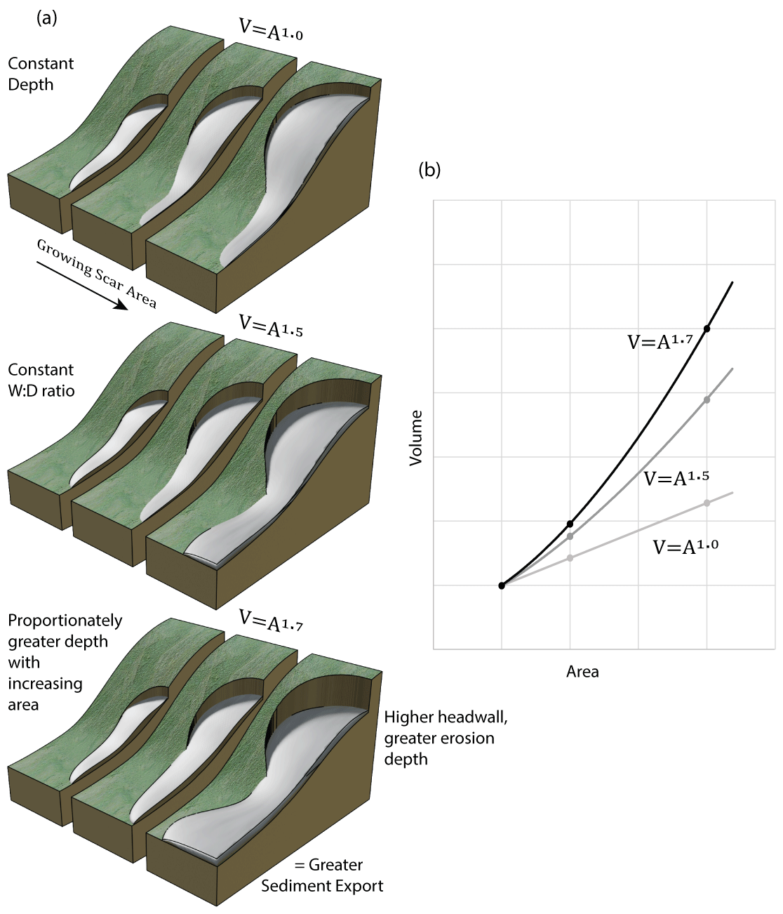
Figure 1Conceptual diagrams of retrogressive thaw slumps showing the influence of area–volume model coefficients on disturbance morphology. The effect of the scaling exponent (δ) is illustrated by the slope schematics (a) and portrayed graphically in (b).
Mass-wasting inventories characterize spatial and size–frequency distributions, providing a basis for determining dominant modes of erosion and estimating the volumetric rates of sediment, chemical, or nutrient mobilization from hillslopes (Oguchi, 1997; Campbell and Church, 2003; Tunnicliffe and Church, 2011; Kokelj et al., 2021). In temperate or mountainous regions, most landslides are rapid, discrete events that take place over a short time frame (seconds to days), so inventory studies typically assume a temporal window of relevance where the scar remains visible before being forested over (Brardinoni et al., 2003). In contrast, retrogressive thaw slumps are chronic sites of thaw-driven erosion that modify slopes over months, years, decades, or even millennia (Burn and Friele, 1989; Lantuit and Pollard, 2008; Lacelle et al., 2010, 2015). These landslides initiate by mechanical or thermal erosion as small disturbances at the base or break in slope, along flow tracks, or as shallow slides that remove surface insulating materials and expose ice-rich permafrost at the ground surface (Lewkowicz, 1987; Lacelle et al., 2015). Ground ice exposed in the slump headwall melts, causing the disturbance to enlarge and a thawed slurry to accumulate in the scar zone. Thawed materials are transferred downslope seasonally by gradual creep or episodic surface or deeper-seated flows at rates controlled by material properties and volume, local topography, and climate drivers (Kokelj et al., 2015). Warmer temperatures or greater rainfall have accelerated the evacuation of scar zone materials, driving positive feedbacks that maintain the headwall height and upslope growth potential of the retrogressive disturbance (Kokelj et al., 2015, 2021). Variations in terrain factors, the intensity of thaw-driven processes, and climate give rise to a diverse range of disturbance morphologies (Fig. 2b–e). Regardless of the setting or size of the retrogressive thaw slump, the gradual decline in headwall height with upslope growth and material accumulation results in stabilization (Burn and Lewkowicz, 1990). Diffusive processes eventually produce gentle slope-side concavities colonized by luxuriant vegetation that distinguish old thaw slump scars from the adjacent terrain (Lantz et al., 2009). The association of retrogressive thaw slump activity with favourable ground ice, slope, and initiating conditions suggests that stabilized thaw slump scars are good indicators of climate-sensitive slopes (Fig. 2b–e). Indeed, thaw-slump-affected slopes are typically subjected to cycles of periodic activity punctuated by stability (Mackay, 1966; Burn and Lewkowicz, 1990; Burn, 2000; Lantuit and Pollard, 2008; Lantz and Kokelj, 2008; Kokelj et al., 2009). The climate-driven increase in polycyclic behaviour has occurred with the intensification of fluvial, coastal, and thermal erosion, as well as the alteration of slope stability thresholds, which has modified the evolution of permafrost slopes (Kokelj et al., 2015; Ward Jones et al., 2019; Kokelj et al., 2021).
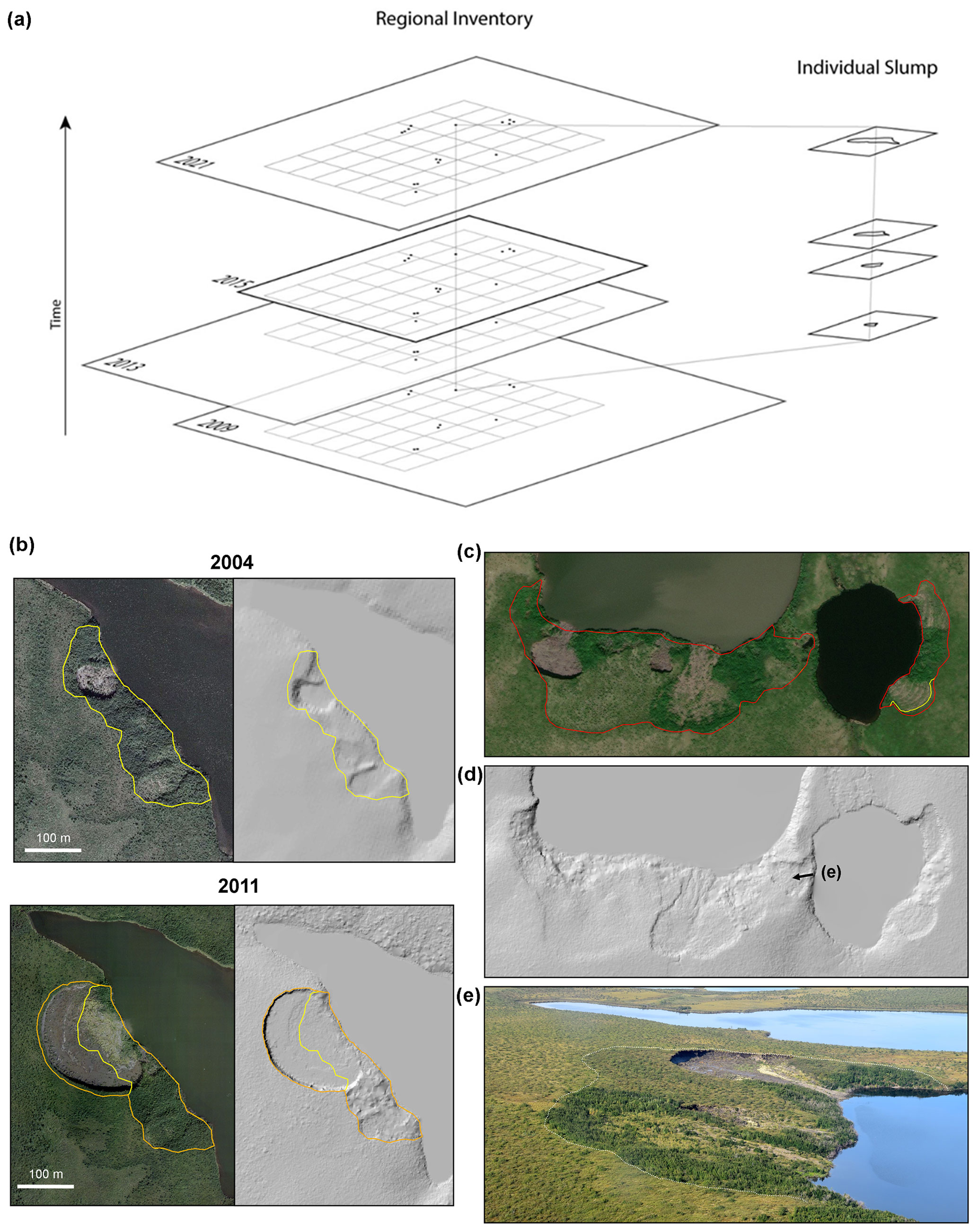
Figure 2Conceptual diagram of the multisource slump inventory (MSI) database and complex lakeside retrogressive thaw slump growth patterns in the Anderson Plain–Tuktoyaktuk Coastlands region. (a) The MSI database incorporates a time series of thaw slump disturbance delineations from several high-resolution DEMs covering variable spatial extents, yielding an integrated data product of landscape change. Panel (b) shows a sequence of DEM-based slump digitization (2004–2011) (68.529∘ N, −133.743∘ W) following the rapid enlargement of a lakeside thaw slump into previously undisturbed terrain. The attribution of the hillshade DEM-based digitizations is supported by high-resolution optical imagery. (c) Polycyclic behaviour of retrogressive thaw slumps showing variously aged disturbances occurring within the footprint of a larger historical disturbance evident in the circa 2016 orthoimagery (World Imagery; ESRI and Maxar), (d) hillshaded 2011 lidar DEM showing distinct and subtle relief of multi-aged disturbance footprints, and (e) oblique photograph from 2020 (68.608∘ N, −133.599∘ W). Slump boundaries represent 2004 (yellow), 2011 (orange), and circa 2016 conditions (red) in panels (b) and (c) to illustrate change between respective DEM datasets (Supplement Sect. S2; Van der Sluijs and Kokelj, 2023).
The planimetric area of active thaw slump disturbances in northwestern Canada span at least 6 orders of magnitude (Kokelj et al., 2021). Small cuspate disturbances with a shallow headwall that retreats upslope have typically affected 0.1 to 1 ha of terrain before stabilizing (Fig. 2b–e). However, climate-driven intensification of thaw has caused disturbances that exceed tens of hectares in area to develop and translocate millions of cubic metres of slope materials to downstream environments (Kokelj et al., 2021). The quantitative metrics change as a disturbance progresses through the stages of geomorphic development or as governing climate conditions change. The dynamic nature of retrogressive thaw slumping suggests that the regional distribution, size, and activity metrics of a permafrost landslide population at any given point in time will reflect the combination of terrain and climate conditions. Digitized spatial datasets yield snapshots of these dynamic disturbance populations (Fig. 2a), but they can vary significantly with project purpose, as well as factors such as slope disturbance definition, the quality and resolution of the underlying base data layer(s), and mapper experience and field-based understanding of periglacial geomorphology in the Anthropocene (Aylsworth et al., 2000; Lantz and Kokelj, 2008; Guzzetti et al., 2012; Segal et al., 2016; Huang et al., 2020; Kokelj et al., 2021). Even if the geomorphic definitions are clear, several challenges inherent to remote sensing remain, such as undetected slumps (i.e., false negatives) and the inclusion of landscape features or noise that are not a thaw slump (i.e., false positives) (Bernhard et al., 2020; Huang et al., 2020; Nitze et al., 2021; Runge et al., 2022). There may also be discrepancies among digitization efforts, where differing delineations are an artefact of disparate data products and slump ontology. These challenges indicate the need for standardized methods to identify, delineate, and attribute thaw-driven landslides, informed by field-based knowledge.
An improved understanding of permafrost landslides also requires advancing a three-dimensional framework for quantifying their geomorphic evolution and environmental impacts. The statistical relationships between landslide scar area and eroded volume provide a foundation for quantifying the geomorphic change (Klar et al., 2011). These relationships are typically expressed as power-law models; they have been explored for a range of failure types, material properties, and geological settings across temperate landslide environments (Larsen et al., 2010; Klar et al., 2011). The volume of material that is thawed by retrogressive thaw slumping scales exponentially with scar area (Fig. 1) (Kokelj et al., 2021), but how these relationships transfer to a diverse array of thaw-driven mass-wasting features across a range of permafrost environments is unknown. Furthermore, since climate can alter the lithological controls on permafrost terrain, it is unclear if these scaling parameters will change as slope stability thresholds and permafrost physical properties are altered by a warmer and wetter circumpolar climate.
An investigation of area–volume () relationships for active thaw slumps in the Beaufort Delta region of northwestern Canada indicated a power-law relationship between area and the total evacuated sediment volume (R2 = 0.9), providing a first quantitative basis for estimating thaw-driven denudation as a function of disturbance area (Kokelj et al., 2021). There are two coefficients in the power-law relationship (Eq. 1) used to predict eroded volume (V) based on planimetric scar area (As): (1) the scaling factor (a), which represents the intercept of the log-transformed linear relationship between disturbance area and volume (Fig. 1a) (Jaboyedoff et al., 2020), and (2) the scaling exponent (δ), which reflects the elastic distortion (or slope) of the area–volume () relation with changing area (Chaytor et al., 2009; Tseng et al., 2013). For example, if the scaling exponent is close to δ= 1, then the thaw slump volume grows primarily with increasing scar area with little to no increase in the absolute scar depth (i.e., linear growth model; Fig. 1a). However, as the exponent approaches δ= 1.5, the relative depth of the concavity grows in proportion to the scar area. Exponents δ > 1.5 reflect slumps that erode more deeply as planform area increases (Fig. 1a). Volume predictions are very sensitive to small differences in the scaling exponent (δ) (Fig. 1b).
The goal of this study is to couple knowledge of thaw slump processes and forms with remote sensing tools to develop more holistic approaches to quantifying and tracking thaw-driven mass wasting, improve the quality of mass-wasting inventories, and refine population-wide estimates of total sediment yield. To accomplish our project goal we (A) evaluate surface interpolation methods necessary to derive slump volume estimates from high-resolution digital elevation models (DEMs); (B) improve slump delineation, morphological descriptions, and activity status using available base maps (lidar, ArcticDEM, satellite imagery); and (C) explore the statistical properties of allometric relationships for a large sample of thaw slump observations (n= 2661) using the results from objectives (A) and (B). The 5948 km2 study area extends across a range of terrain types in the Beaufort Delta region of northwestern Canada. The data and analyses enabled us to explore the uncertainty in volumetric yield estimates, characterize the spectrum of thaw slump morphometry and activity levels across different geomorphic settings, and evaluate area–volume models required to quantify the cumulative landscape effects of climate change.
2.1 Study area
The study area spans the Peel Plateau (Kokelj et al., 2017b), Anderson Plain, lower Mackenzie Plain, and Tuktoyaktuk Coastlands physiographic regions (Rampton, 1988; Burn and Kokelj, 2009). The terrain contains abundant excess ground ice in the form of segregated (Rampton, 1988; Burn, 1997), relict (Murton, 2005; Lacelle et al., 2019), and wedge ice (Mackay, 1990; Kokelj et al., 2014). The spatial distribution of slumps in this region confirms the abundance of ice-rich permafrost and the overall sensitivity of ice-marginal, permafrost-preserved glacigenic terrain (Kokelj et al., 2017a).
We examined two specific study areas: (1) the lake-rich rolling tundra of Anderson Plain and Tuktoyaktuk Coastlands (APTC) (Rampton, 1988) with an area of 3278 km2 and (2) the fluvially incised Vittrekwa and Stony Creek watersheds of the Peel Plateau (PP) (Kokelj et al., 2017b) with an area of 2670 km2. These regions host the communities of Tuktoyaktuk, Inuvik, and Fort McPherson; the Dempster and Inuvik to Tuktoyaktuk Highway corridors; and the greatest density of historical oil and gas infrastructure in Arctic Canada (Fig. 3) (Burn and Kokelj, 2009).
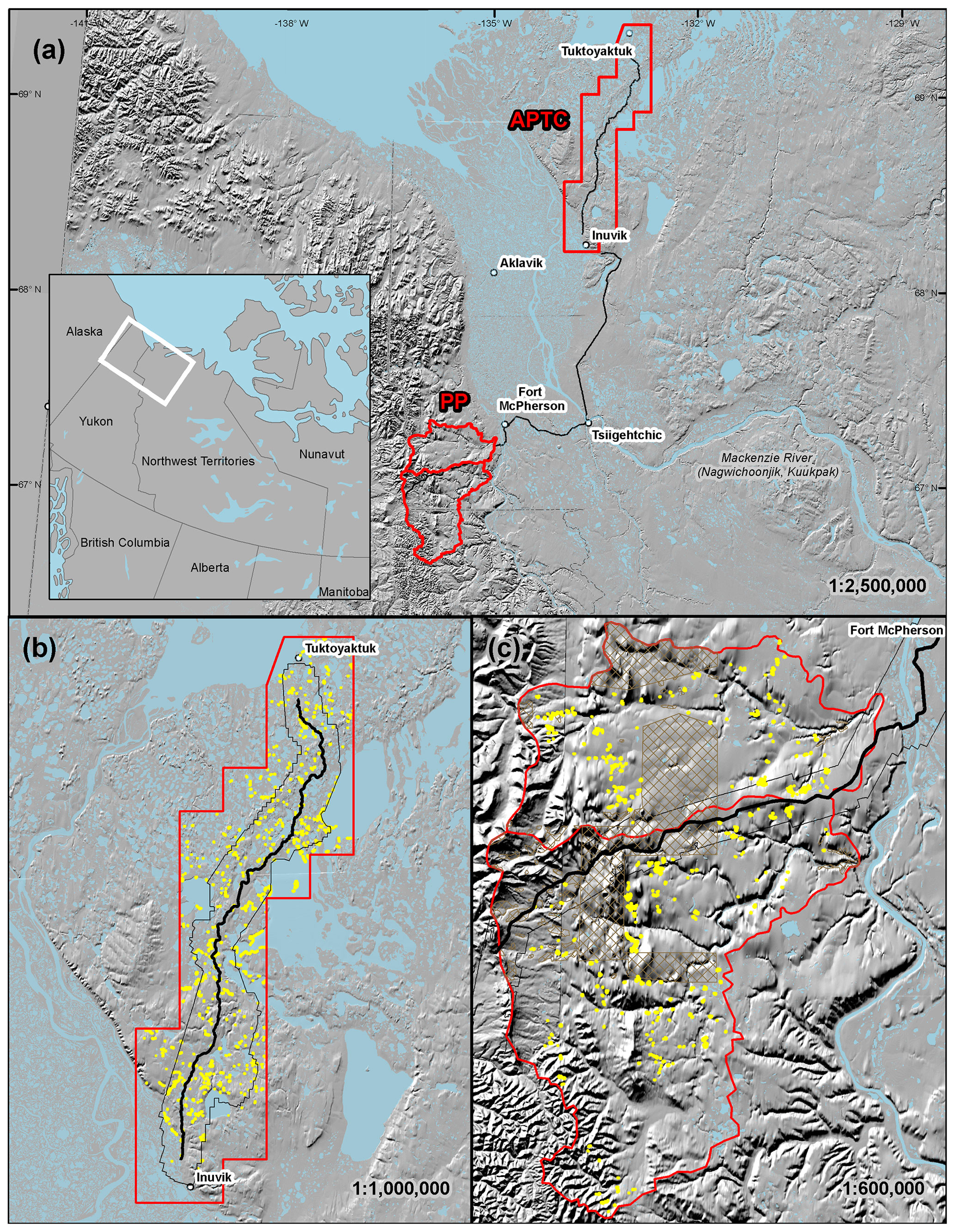
Figure 3Map of study areas (a) and DEM-based digitization of circa 2016 slumps (yellow) in the Anderson Plain–Tuktoyaktuk Coastlands (b; APTC) and Peel Plateau (c; PP; Vittrekwa and Stony Creek watersheds). Basemap is a 1:250 000 hillshaded Canadian DEM (CDEM; Natural Resources Canada 2013 – Open Government License). Black lines define the highways (bold) and lidar extents (narrow). ArcticDEM tiles for the PP area included data voids (brown crosshatch; totalling 510 km2; Porter et al., 2018).
2.2 Study design
This study developed methods of characterizing thaw-driven landslides to estimate disturbance volumes so that geomorphic impacts can be quantified. The study builds on a long-term permafrost research and landscape change monitoring program by the NWT Geological Survey and its research partners in the Mackenzie Delta region (Kokelj et al., 2005, 2009, 2013, 2015, 2017a; Lacelle et al., 2015; Lantz and Kokelj, 2008; Lantz et al., 2009; Van der Sluijs et al., 2018; Sladen et al., 2021; Kokelj et al., 2021). The improvement in mapping methods leveraged geomorphic knowledge of the study area, existing landslide inventories (Segal et al., 2016), and high-resolution orthomosaics and DEM datasets obtained over the past decade and a half (Table 1). The first objective (A) was to determine the uncertainty in surface interpolation methods used to reconstruct pre-erosion hillslope morphology (Table 1a). The second objective (B) was to improve methods to detect, delineate, and characterize retrogressive thaw slumping (RTS)-affected terrain using high-resolution DEMs and optical imagery and develop a multi-temporal dataset of disturbances (Table 1b) to explore the variation in morphology and activity levels of slump-affected terrain. Utilizing this DEM-derived disturbance dataset (objective B) and applying the best interpolation method determined in objective A, we derived area–volume relationships for a large population of thaw slump disturbances and determined morphological and terrain factors that contribute to scatter in the relation (Table 1c). A method flowchart detailing these inter-related workflows is shown in Supplement Fig. S1.
Table 1Summary of research goals, remote sensing datasets and related methods sections, geographic locations, and sources of the datasets used in this study.
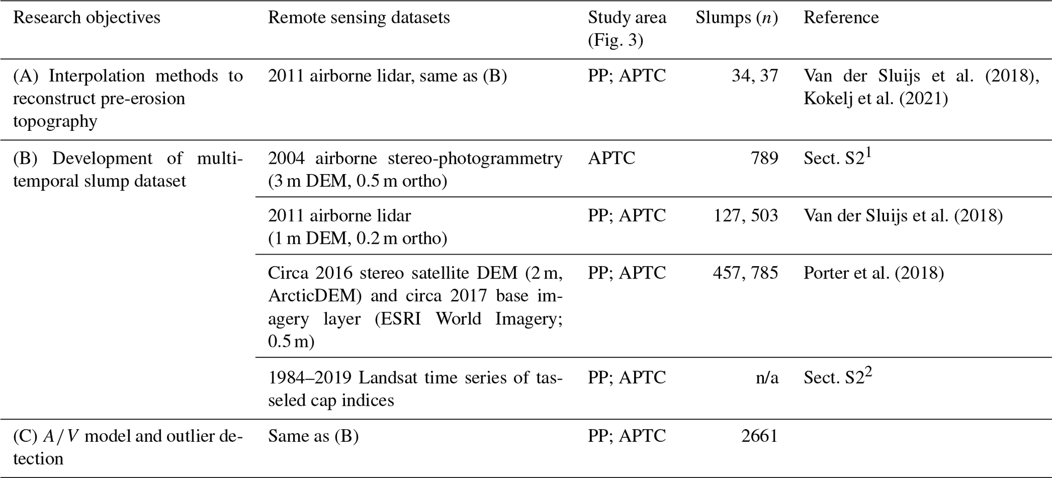
1 Mackenzie Valley Air Photo (MVAP) project of Indian and Northern Affairs Canada, now Government of Northwest Territories with NWT Centre for Geomatics as publisher. 2 Method based on Fraser et al. (2014). Note that n/a stands for not applicable.
2.2.1 Pre-disturbance terrain methods
The volume of a thaw slump scar is the product of thaw subsidence from thermoerosion and ground ice loss (Lewkowicz, 1987), as well as downslope sediment transport (Kokelj et al., 2015, 2021; Figs. 2, 3). The volume of materials displaced by thaw slump activity can be estimated through DEM differencing (Lantuit and Pollard, 2008; Van der Sluijs et al., 2018; Kokelj et al., 2021; Turner et al., 2021). In cases where both DEMs reflect hillslopes in the disturbed state, the derived difference reflects the episodic denudation (e.g., inter-survey), whereas the total denudation volume loss of a thaw slump can be determined if a “pre-disturbance” DEM is available (i.e., since initiation of the feature). Typically these multi-decadal disturbances predate high-resolution DEMs, requiring reconstruction of the disturbed topography through manual or semi-automated DEM void-filling techniques (ten Brink et al., 2006; Van der Sluijs et al., 2018; Kokelj et al., 2021). To build robust regional slump volume datasets we investigated the effectiveness of surface interpolation methods for obtaining pre-disturbance DEMs and compared how well the reconstructed ice-rich permafrost terrain surfaces conform to the original topography. To develop a dataset that would enable us to evaluate the performance of interpolation methods, we generated a series of slump-shaped data voids that were randomly placed on undisturbed terrain considered conducive to slump development within the 2011 lidar DEM extents (Lacelle et al., 2015; areas with 2–12∘ slopes and within the maximum extent of the Laurentide Ice Sheet). We used the digitizations and size distribution of active-slump populations in fluvially incised settings to generate random void areas in the PP study area (n= 34, Kokelj et al., 2021). The randomization was iterated 30 times so that the 34 voids were each positioned in 30 different terrain locations. A similar approach was applied to assess reconstruction fidelity within predominantly lacustrine environments in the APTC area (n= 37; Kokelj et al., 2021). Data voids were only retained if the random placement was within 400 m of a lake. These procedures produced a dataset consisting of 1020 voids for the PP area (n= 34 slumps and 30 iterations) and 359 voids in the APTC area (study total n= 1379).
The magnitude of interpolation error can vary considerably among methods due to underlying model assumptions, parameterization, sensitivities to the quality of the input data, and the morphologic setting of the void (Reuter et al., 2007; Bergonse and Reis, 2015; Boreggio et al., 2018). Eight interpolator suites commonly available and described in GIS software manuals and used for digital terrain modelling (ArcGIS Pro™ v.2.7) were identified to reconstruct the synthetic DEM data voids: (1) inverse distance weighted (IDW), (2) TIN-to-raster (TR), (3) regularized spline with low weights (RSL), (4) regularized spline with high weights (RSH), (5) spline with tension (ST), (6) empirical Bayesian kriging with no data transformation (EBK), (7) EBK with empirical data transformation (EBK-EMP), and finally (8) EBK with empirical transformation and detrended semivariograms (EBK-EMPD). The eight different interpolation suites were tested with a range of parameterizations (a total of 32 interpolation methods; Table S2) to assess performance within and between methods. The topography of each void was reconstructed independently following an automated Python workflow (S4) that buffered each void by 50 m, retained the pixels outside of the void, and converted them to boundary elevations that were used by each of the 32 interpolation methods. Then re-interpolated void surfaces (n= 1379) were compared with the original lidar terrain surface to test the accuracy of surface interpolators (Reuter et al., 2007). Elevation differences between true (actual lidar DEM) and modelled (interpolated terrain) elevations were summarized for each void by calculating the root mean square difference (RMSD), mean absolute error (MAE), and the summed absolute topographic difference (Tsum). In this case, the RMSD is a measure of error (in metres) describing how well the modelled terrain fits the actual terrain. MAE measures the average absolute difference of the error. Tsum is an indicator of three-dimensional topographic uncertainty expected for a reconstructed void surface (in m3), with 0 m3 reflecting a perfect fit. Non-parametric statistical testing (Kruskal–Wallis and Dunn's post hoc tests with Bonferroni adjustment) was implemented to assess potential differences in RMSD between interpolator suites and between individual methods.
2.2.2 Multisource slump inventory (MSI)
Slump disturbances were identified and digitized at very large mapping scales (> 1:2000) utilizing compilations of the best available high-resolution hillshade DEMs (≤ 3 m; see Sect. S2 for dataset details) and imagery (≤ 0.5 m). Due to the evolving nature of thaw slumps, an approach based on a “multi-temporal inventory map” (Guzzetti et al., 2012) was pursued, namely the multisource slump inventory (MSI). The MSI approach was implemented to (1) acquire temporally consistent, high-resolution digitizations for each slump-affected slope area based on the best available DEM (Fig. 2a); (2) obtain more descriptive information on the geomorphic activity to better track disturbance evolution by inspecting high-resolution imagery; and (3) reduce the number of small undetected, inactive, or shallow slumps, as is typically the case with landslide inventories (Stark and Hovius, 2001; Guzzetti et al., 2012). The hillshade DEMs in this study enabled the detailed digitization of disturbances and numerous revegetated stable slump scars to be identified and mapped with greater confidence, which has been constrained in the past when using optical or coarser base data layers (Fig. 2d). The MSI included mapping partially or fully vegetated old and ancient slump scar areas because they are important indicators of ice-rich thaw-sensitive terrain (Fig. 2b–e) (Kokelj et al., 2009). Steps were undertaken to integrate the datasets (Fig. 2) by applying delineation rules formulated for partial or fully stabilized slumps as well as highly polycyclic slumps. These MSI methods are described in detail in Van der Sluijs and Kokelj (2023), so only a brief summary is provided here. The delineation rules were based on (1) iterative delineation with reference to past data, (2) a slump feature not being allowed to drop out of the inventory after detection, and (3) slump-disturbed areas only being able to increase through time (with the exception of areas with shoreline erosion). Each delineated feature was attributed by landscape descriptors, two-dimensional geometry estimates, and three-dimensional hypsometry estimates, along with a characterization of activity levels based on surface area percentage of activity (in 10 % increments) using visual clues in the optical imagery and hillshaded DEM (Table 2; Fig. 6c; Van der Sluijs and Kokelj, 2023). Percentages were also grouped into three classes to facilitate summary statistics among stable slumps (0 %), minimally active slumps (10 %), and moderately to highly active slumps (20 %–90 %). It should be noted that the total slump-affected area of disturbances in the MSI may not change if the recent activity is taking place entirely within the footprint of an older disturbance (Fig. 2c). However, in such instances the percent activity estimates would indicate an intensification of slumping (e.g., from a 0 % inactive slump to a 20 % reactivated slump). The “active surface area” of an individual disturbance was based on the total slump-affected area multiplied by the estimated percentage of the active area.
Table 2Summary of slump geomorphic attributes included in this inventory.
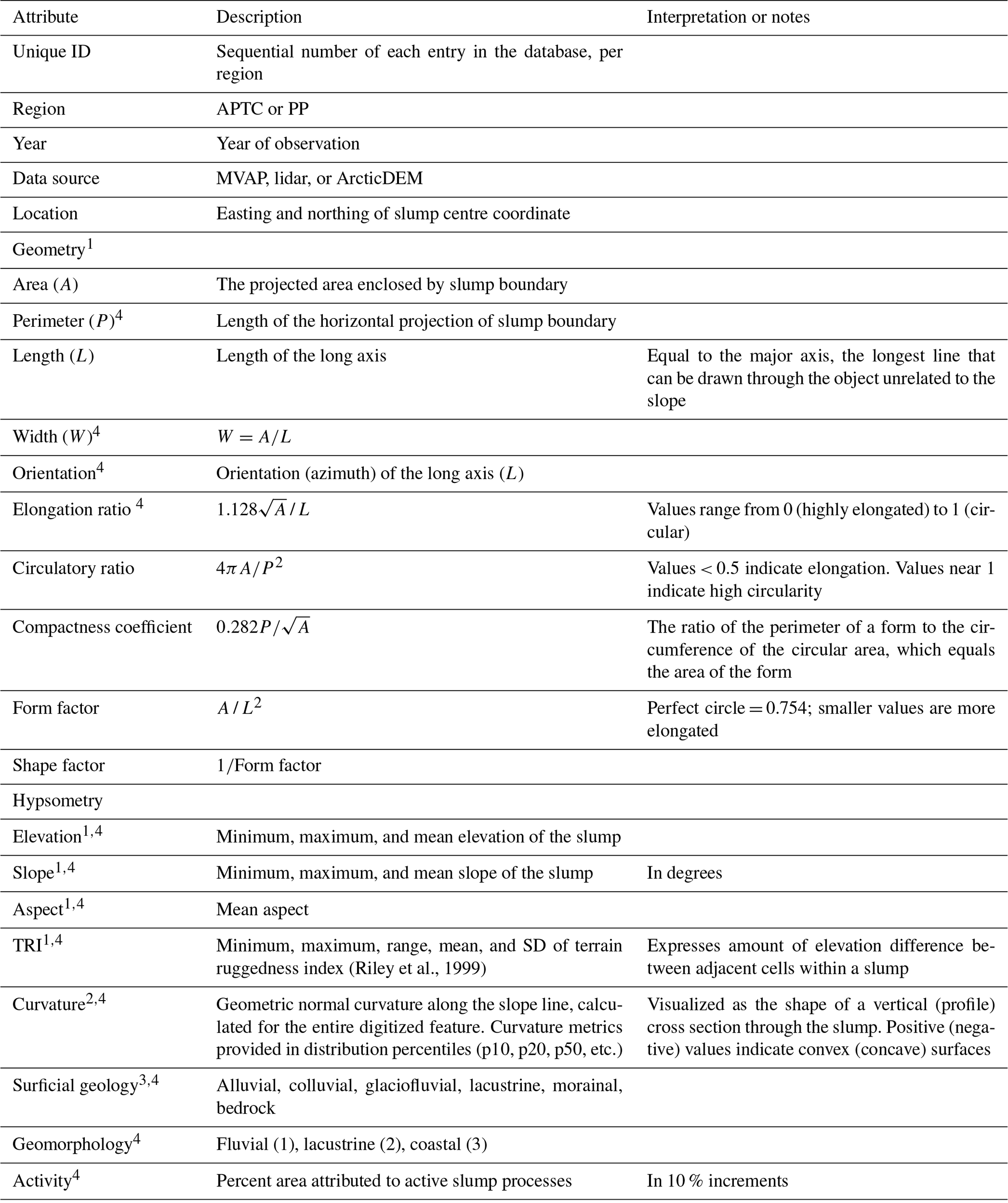
1 Derived using Morphometry Assessment Tools for ArcGIS (Gudowicz and Paluszkiewicz, 2021). 2 Derived using Surface Parameters tool in ArcGIS Pro based on 10 m neighbourhood distance. 3 Derived from Smith and Duong (2012) and Côté et al. (2013). 4 Variable used in random forest modelling after removal of highly correlated variables (Sect. 2.2.3).
2.2.3 Area–volume () allometry and outlier detection
In this study, we explored relationships between thaw slump area and two distinct volume parameters. First, we examined relationships between slump area and the difference between real and modelled slump topography (Tsum) to determine the uncertainty of reconstructed surfaces and how these scale with slump area (objective A). The slump area dataset consisted of a randomly placed population of slump voids following procedures described above (Sect. 2.2.1), with uncertainty in the surface reconstruction expressed in both absolute and relative terms. Secondly, we explored the relationships between slump area and total evacuated sediment volume (objective C): the latter parameter was derived by differencing slump-affected DEMs from the modelled pre-disturbance DEMs determined using the best performing interpolator (objective A). For this analysis, data on slump area, activity level, and disturbance volume from the MSI (objective B) were analysed in a multiple linear regression framework. Slump area and volume data were logarithmically transformed to meet assumptions of normality. The software package R Statistics (v. 4.0.2) was used to produce descriptive statistics and regression analyses. Slumps were digitized from up to three different periods, according to the availability of various DEM data sources. Temporal auto-correlation between multiple observations of the area, activity level, and volume for the same slump in the MSI dataset was addressed in the multiple regression by including a categorical “data source” term in the models (Table 2).
We explored model performance and residuals to determine whether the nature of the outliers could be described to inform constraints on the model's application. Areas affected by thaw slumping that yielded problematic volume estimates were identified as (1) thaw slumps where the modelled pre-disturbance elevations were lower than post-disturbance elevations, producing an incorrect positive volumetric change, and (2) thaw slumps with a correct negative mean depth of thaw and volume but with a volume estimate below the Tsum uncertainty threshold, determined from testing surface interpolation methods described in Sect. 2.2.1. The morphometry and geomorphic setting of the volumetric outliers were examined in a random forest (RF) classification (Breiman, 2001) to explore the attributes that most commonly distinguished these volumetric outliers relative to the entire thaw slump population. In our analysis, RF was used in a binary schema to separate volumetric inliers from outliers using the randomForests package in R, based on a randomly balanced selection of 80 % of the MSI observations (n= 2130, retaining 20 %, or 531 observations, for independent validation), 1000 trees, and 6 explanatory variables randomly sampled at each split. Highly correlated explanatory variables from the MSI, defined as an absolute Spearman's correlation of 0.75 or higher, were removed before classification (Table 2). The influence of the three explanatory variables identified by RF variable importance with the largest overall impact on accuracy was assessed using partial dependence plots showing the probability of being classified as a volumetric inlier or outlier.
3.1 Pre-disturbance terrain methods
To determine the most desirable interpolation techniques for reconstructing terrain surfaces affected by thaw slumping, we examined the performance of 32 surface interpolation methods by comparing differences between observed (actual) and modelled (interpolated terrain) surfaces for 1379 terrain voids representing a population of simulated slump disturbances in the study regions. Interpolation performance is parameterization-dependent, so methods were grouped into suites to identify variation in accuracy associated with general algorithmic implementations. Kruskal–Wallis test results indicated significant differences in RMSD distributions between interpolator suites (H(7) = 7637, p < 0.001). The TIN-to-raster (TR) suite exhibited the lowest RMSDs (median: 0.3 m; 90th percentile: 1.0 m; Fig. 4a), while empirical Bayesian kriging (EBK) with data transformation and detrended semivariograms (EBK-EMPD) achieved the second-lowest RMSDs (median: 0.4 m; 90th percentile: 1.8 m; Fig. 4a). Dunn's post hoc tests indicated that TR's RMSD distribution was significantly different from all other suites (p < 0.001). For all interpolator suites, the RMSD increased non-linearly with the void area, with the TR suite exhibiting the most gradual increases (Fig. 4b). Even though RMSD increased with void size for all suites, relative uncertainties for all interpolators declined with the void area (Fig. 4c). We further evaluated the natural neighbours (NNs) and linear (LIN) parameterizations within the TR suite. Statistical testing indicated that RMSD (H(1) = 2.25, p= 0.133), mean absolute error (MAE) distributions (H(1) = 2.26, p= 0.132), and summed topographic difference distributions (Tsum; H(1) = 0.145, p= 0.703) were not significantly different from one another but were significantly different from parameterization results in all other interpolation methods (Table S2, Figs. S2, S3). These findings show that the NN had the most robust performance for reconstructing topography affected by active retrogressive thaw slumping in fluvially incised glaciated permafrost terrain.
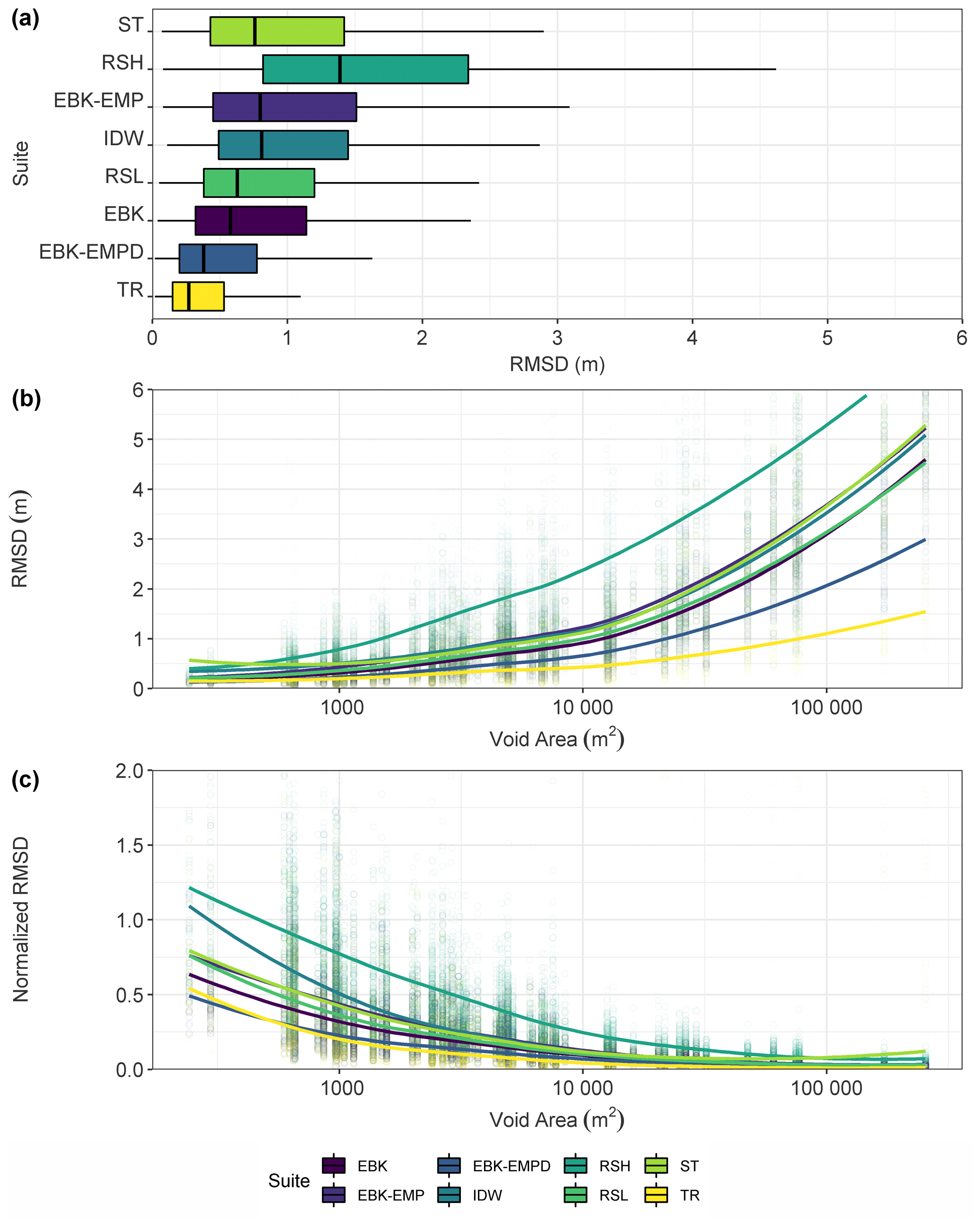
Figure 4(a) Boxplot of differences between actual and modelled elevation (expressed as root mean square difference – RMSD) for each interpolator suite, (b) scatterplot between void surface area and RMSD with smoothing line indicating area-dependent uncertainty of the respective interpolator suites, and (c) scatterplot between void area and normalized RMSD (RMSD/area ⋅ 1000) with locally estimated scatterplot smoothing (loess) line indicating how relative uncertainty of the respective interpolator suites varies with the void area. Together these graphs indicate that the TIN-to-raster (TR) suite of methods (LIN, linear, or NN, natural neighbour, interpolation) achieved the lowest RMSDs among the interpolation suites and exerted the weakest influence of void surface area on RMSD for both study areas. Despite outliers associated with the more poorly performing suites, we restricted the x axis to better visualize the data associated with the best performing interpolator suites.
Using the measure of void area and summed topographic difference (Tsum), the precision of interpolated surface estimates for a given disturbance area could be determined, and an uncertainty estimate could then be assigned to the modelled slump volumes. The synthetic disturbances were grouped into three void area classes, and as anticipated, there were significant increases in Tsum with increasing void area (H(2) = 839, p < 0.001; Fig. 5a). Figure 5b shows a linear model fit through the logarithmically transformed void area (As) and summed topographic difference estimates (Tsum), which is described by a power-law relationship (Eq. 2).
Applying Eq. (2) to the real-world slump samples from Kokelj et al. (2021) indicated that the influence of pre-disturbance interpolation on derived slump volume estimates was relatively small, with uncertainties < 10 % for large slumps and typically within 10 %–20 % of small to medium disturbances (Fig. 5c), which is expressed as an inverse association between slump volume and relative volumetric error (Fig. 5d).
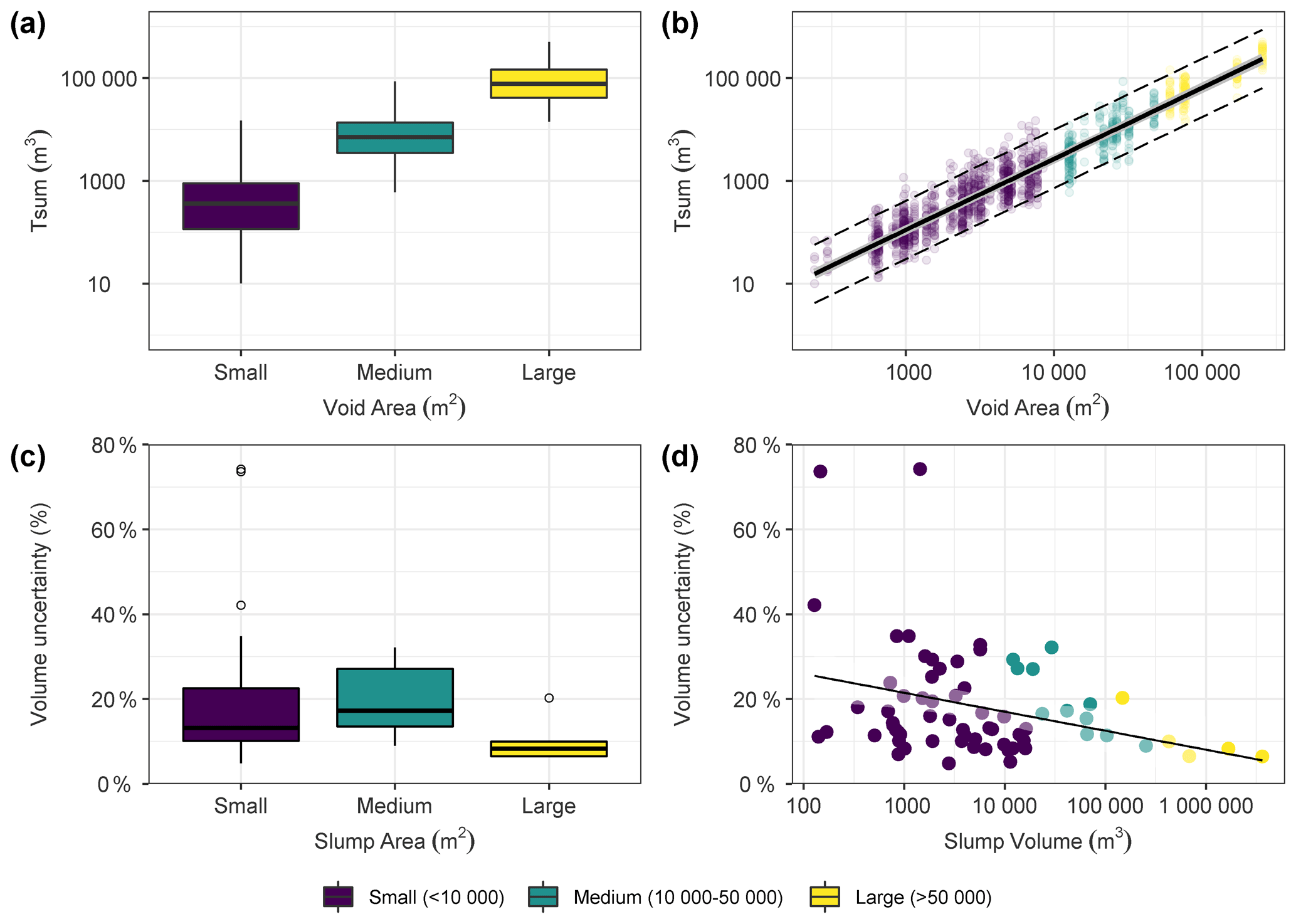
Figure 5Results showing performance of the NN interpolator in modelling pre-disturbance terrain. (a) Box-and-whisker plots showing medians and 25 % and 75 % quantiles of summed topographic difference by void area class. (b) Relationship between void area and summed topographic differences (Tsum). The regression is described by Eq. (2) with a 95 % prediction interval for future observations (dashed lines). (c) Box-and-whisker plots showing medians and 25 % and 75 % quantiles of volumetric difference expressed as a percentage based on modelled volume of thaw slumps. (d) Relationship between modelled slump volume and relative volumetric uncertainty based on data from Kokelj et al. (2021).
3.2 Multisource slump inventory (MSI)
The digitization and attribution of slump-affected terrain utilizing 2016 DEMs and following MSI methods are summarized for the two study areas (n= 1242) (Fig. 6). The activity levels of slopes affected by thaw slumping are characterized by similar cumulative distribution functions for the two study regions (Fig. 7a). In PP and APTC regions 40 % to 60 % of the digitized slump-affected areas were classified as inactive, and an additional 20 %–30 % of disturbed areas were estimated to have only 10 % geomorphically active surface (Fig. 7a). Between 80 % to 90 % of the digitized features were characterized by bare, geomorphically active surfaces contributing less than 20 % of the total scar area. In many cases, active headwall retreat was associated with a small, cuspate-shaped active scar zone comprised of mud slurry and a larger vegetated accumulation zone on the middle and lower slope where materials had accumulated (Fig. 6c). This common thaw slump morphology is contrasted by the fewer, highly active disturbances with high headwalls and dynamic scar surfaces, where large volumes of material are being actively transported from the slope to a downstream environment (Fig. 6c). Singular scars can grow into major “complexes” with multiple lobate scar zones. These geomorphically distinct features are orders of magnitude larger in size, yielding deep cavities and significant downslope debris tongue deposits. They reflect a tipping point in the thaw-driven evolution of ice-rich terrain and have been referred to as “mega slumps” (Kokelj et al., 2015).
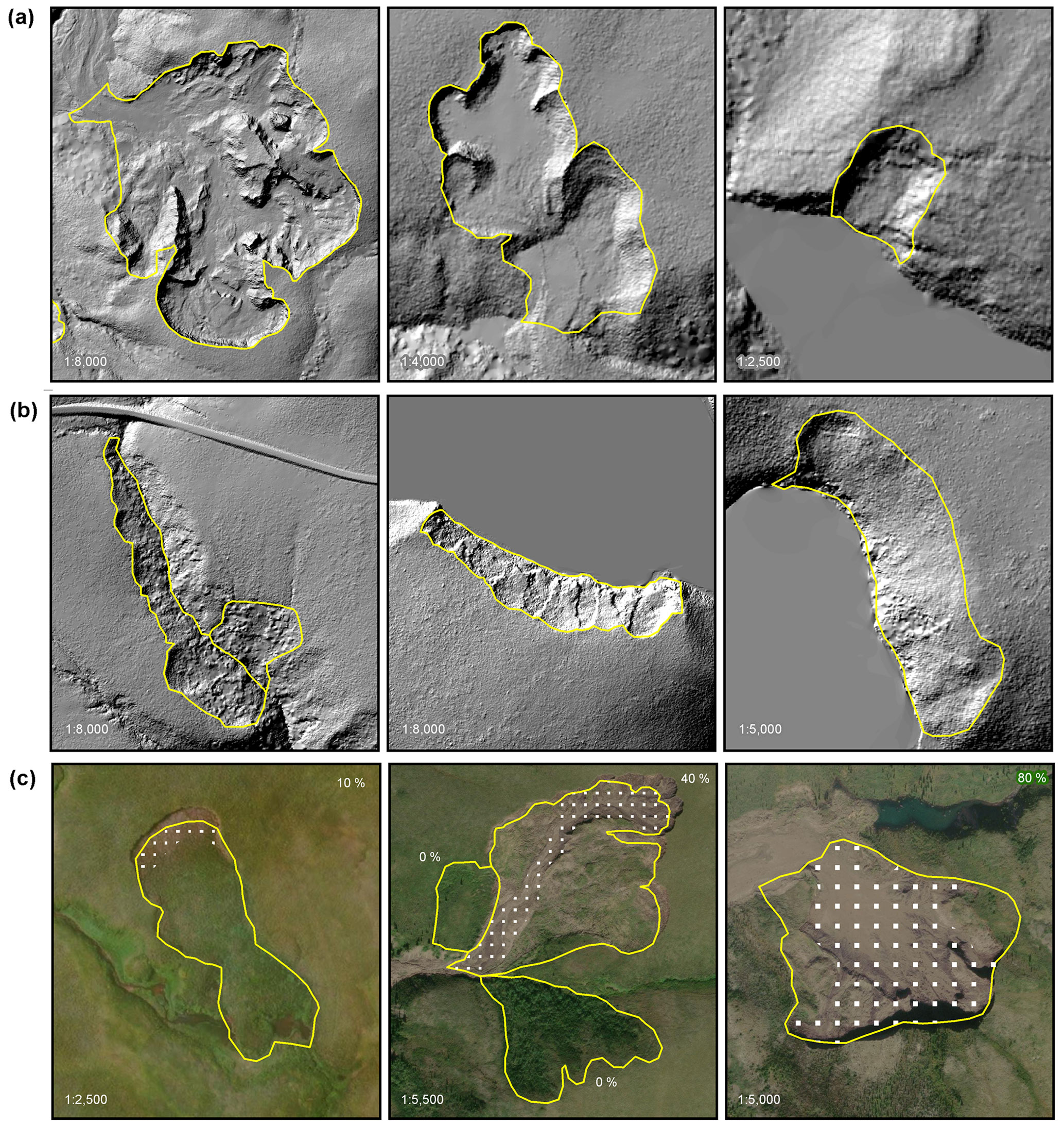
Figure 6Slump form, activity ratings, and morphological variability as documented in the MSI. Morphological and environmental differences between active slumps with compact scar zones and inactive slumps with highly elongated scar zones are shown on 2011 hillshade DEM in panels (a) and (b), respectively. In panel (c) PP slumps are shown exhibiting various activity levels circa 2016 conditions (World Imagery; ESRI and Maxar). In cases of small lateral differences in headwall positions between hillshade ArcticDEM and ESRI World Imagery, the final boundaries were digitized based on hillshade ArcticDEM because elevations outside the slump scar zone were used for pre-disturbance surface interpolation (Sect. 3.1). The extent of white dots in (c) indicates the surfaces affected by active mass-wasting processes used to estimate percent activity.
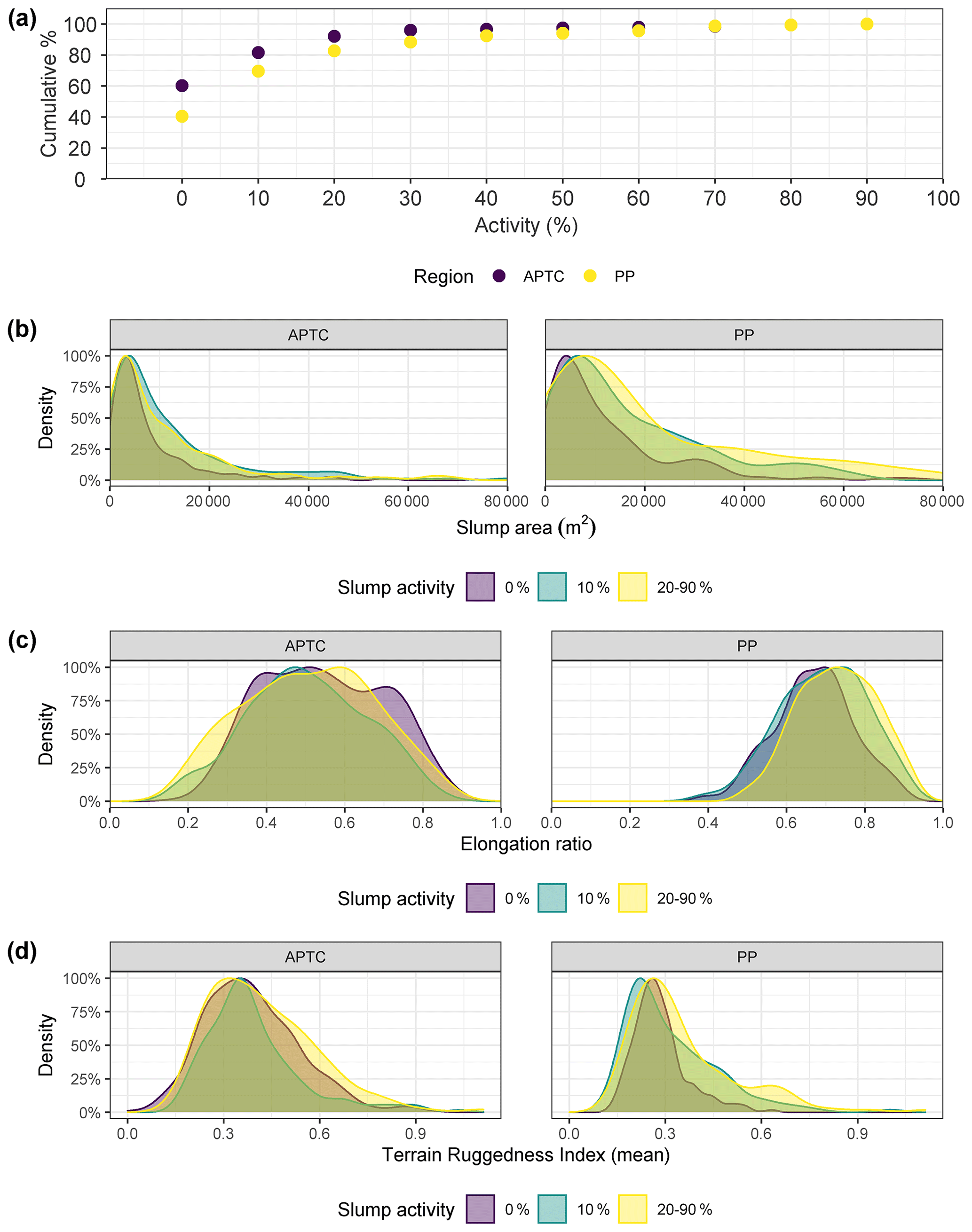
Figure 7The circa 2016 summary statistics showing the (a) cumulative distribution of slump count by activity rating for the two study regions. Panels (b)–(d) show frequency density plots of (b) scar zone area, (c) elongation ratio, and (d) terrain ruggedness (TRI), stratified by the activity levels of slump-affected terrain, for the two study regions.
In the APTC study area 785 features defined as thaw-slump-affected areas were digitized (24.0 slumps per 100 km2), but only 40 % or 313 (9.5 slumps per 100 km2) areas are sites where the processes of retrogressive thaw slumping were active. For the PP study area, 457 features were digitized in areas where ArcticDEM was available (21.1 slumps per 100 km2; Fig. 3), with 272 active features (12.6 per 100 km2), or 60 % of the total population. When slumps with ≤ 10 % active area were removed, disturbance density decreased further to 4.4 per 100 km2 for APTC and 6.4 per 100 km2 for PP. Taken together the MSI statistics highlighted that in 2016 the majority of slump-affected slope areas in the APTC and PP regions consisted of entirely stabilized disturbances or areas of active thaw slumping within the footprint of a much larger, geomorphically inactive disturbance area.
Multi-temporal results for the APTC region demonstrated that the MSI helps in linking field-based observations of the slump process to a digital inventory intended to track the area, volume, and dynamics of thaw-driven landslides through time. Figure 8a and b show that the regional density of thaw slumps (24.1 slumps per 100 km2 in 2004 to 24.0 slumps per 100 km2 in 2016) and total disturbed area of thaw-slump-affected terrain (23.7 ha slump-affected terrain per 100 km2 to 24.7 ha slump affected terrain per 100 km2) varied little between 2004 and 2016 (+3.5 %). However, the regional density of active thaw slumps (activity ≥ 0 %) increased by 38 %, from 6.9 slumps per 100 km2 in 2004 to 9.5 slumps per 100 km2 in 2016, and the estimated area affected by active slumping increased by 69 %, from 1.4 ha per 100 km2 to 2.4 ha per 100 km2. The density of moderate to highly active slumps increased by 49 %, from 3.0 slumps per 100 km2 to 4.4 slumps per 100 km2. The results reinforce that slump activity in the APTC region between 2004 and 2016 increased and occurred within areas of past disturbance.
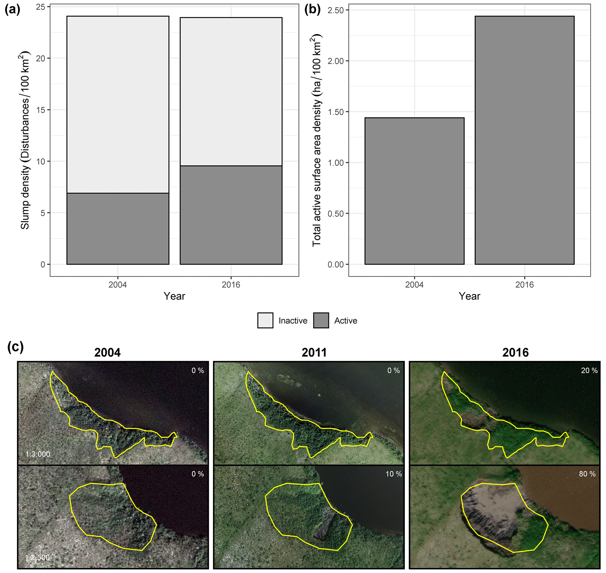
Figure 8Temporal change in (a) count and (b) total active area of slump-affected terrain in the APTC study region documented by MSI methods. (c) Examples of APTC slump activity levels and trends in the MSI, where past disturbances are reactivated (World Imagery; ESRI and Maxar).
We also use the MSI dataset to examine variation in the morphology of RTS-affected terrain across the study regions. Slump area varied between regions and among slump activity ratings (Kruskal–Wallis H(5) = 109, p < 0.001). As reported in Kokelj et al. (2021), slumps in the PP region were on average larger than those in the APTC region and exhibited a greater standard deviation (Table 3; Fig. 7b). Dunn's post hoc tests indicated that disturbance areas with active slumping were significantly larger than completely stable scar areas in each region (Table 3). Statistical distributions of elongation ratio, expressing the overall plan form of the disturbance, were also significantly different between regions and among slump activity ratings (Kruskal–Wallis H(5) = 322, p < 0.001). Slump-affected areas predominantly in the PP region had considerably higher elongation ratios (medians ranging between 0.67–0.73) compared to the lacustrine or coastal slumps located in the APTC region (medians: 0.50–0.54). A higher ratio indicating a more circular or compact morphology increased with slump activity level in the PP (Fig. 7c). Activity level did not have the same influence on the morphometry of shoreline disturbances in the APTC (Table 3). Hypsometric indices derived from the DEM also varied between regions and activity groups. For example, statistical distributions of the terrain ruggedness index (TRI; Riley et al., 1999), describing the amount of local terrain relief in a slump, were significantly different between regions and among slump activity ratings (Kruskal–Wallis H(5) = 135, p < 0.001). However, significant differences in TRI were only observed at the regional PP versus APTC level and furthermore only among PP slumps grouped by activity (Table 3). The highest average TRI values were observed for moderate to highly active slumps (Fig. 7d). These observations highlight diversity in the morphology of slump-affected terrain, which varies with region and activity level, and when stable and larger polycyclic disturbance footprints are delineated, complex morphologies beyond the simple, cuspate slope disturbance form emerge.
Table 3Summary statistics for select two- and three-dimensional metrics of the MSI*.
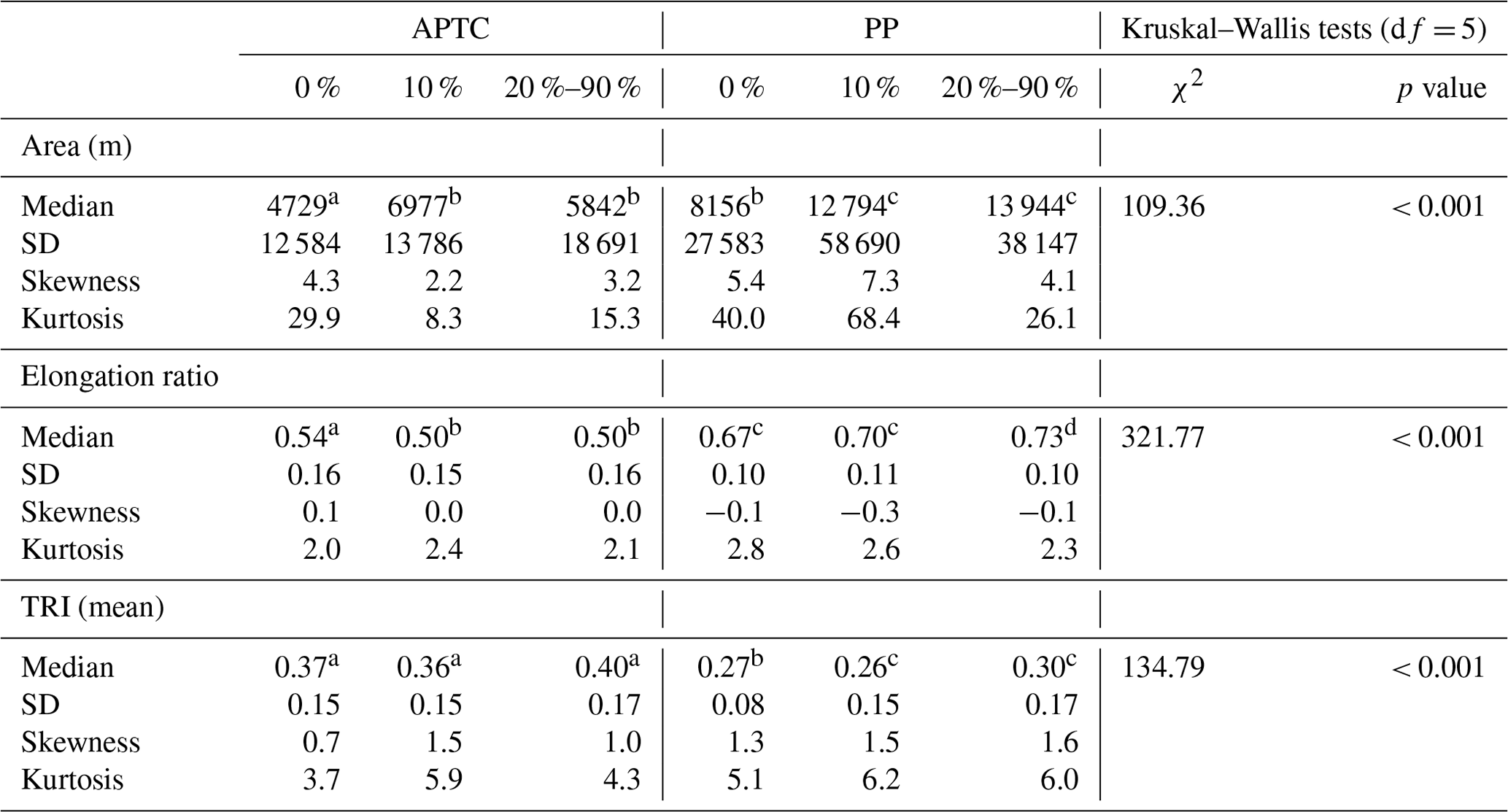
* Coding (a, b, c, d) with letters of the groups that are significantly different based on Dunn's post hoc.
3.3 Area–volume () allometry and outliers
We evaluated the area–volume relationship for a large population of thaw slumps in the two study areas (Fig. 1), utilizing disturbance area and activity attributes from the MSI, as well as the volumes estimated by differencing the disturbed terrain surfaces against the modelled pre-disturbance DEMs derived using the NN interpolator (Fig. 5). Digitized slump area was the continuous predictor variable, and percent activity and data source were categorical variables used to model scar volumes of slopes affected by retrogressive thaw slumping (Table 2). Volume estimates that yielded a negative value indicating an increase in terrain relief (n= 855), which is not possible, were omitted from this analysis, yielding a total sample of 1806 slump-affected areas with an associated disturbance volume. The resulting model, with an adjusted R2 model fit (adj-R2) of 0.66 (p < 0.001), was characterized by non-normally distributed residuals, heteroscedasticity, and data points that unduly influenced the relationship (Table 3, model no. 1). Both data source and percent activity were found to be significant explanatory variables (p < 0.001; Table 3). Exclusion of the data source and activity terms did not appreciably affect the adj-R2 or change the scaling coefficients or regression diagnostics of the simplified model described by Eq. (3) (adj-R2 of 0.65; Table 3, model no. 2; Fig. 9a). These model results and diagnostics highlighted the challenges of thaw slump volume predictions for complex disturbances that occur across a diverse range of terrain, slump morphologies, and activity levels captured by the MSI.
To better understand the application and limitations of the models for predicting geomorphic change and volume of permafrost thawed as a result of retrogressive thaw slump disturbances, we explore the characteristics of outliers and inliers in the relationship described by Eq. 3 (Fig. 9a). The initial MSI inventory of the study areas yielded 2661 observations of slump-affected terrain, but the NN re-interpolation procedure resulted in 855 occurrences of terrain surface estimates predicting a net positive change in post-disturbance surface elevation rather than the surface lowering, which is the logical result of retrogressive thaw slumps in ice-rich terrain. Therefore we determined outliers as thaw slump disturbance areas characterized by incorrect, positive estimates of disturbance volumes (n= 855), as well as those disturbances with a volume estimate that did not exceed the Tsum uncertainty threshold defined by the relationship shown in Fig. 5b and Eq. (2) (n= 284). By this criteria, inliers were slump-affected areas with modelled volumes exceeding the uncertainty threshold associated with terrain surface reconstruction (Fig. 5b, n= 1522).
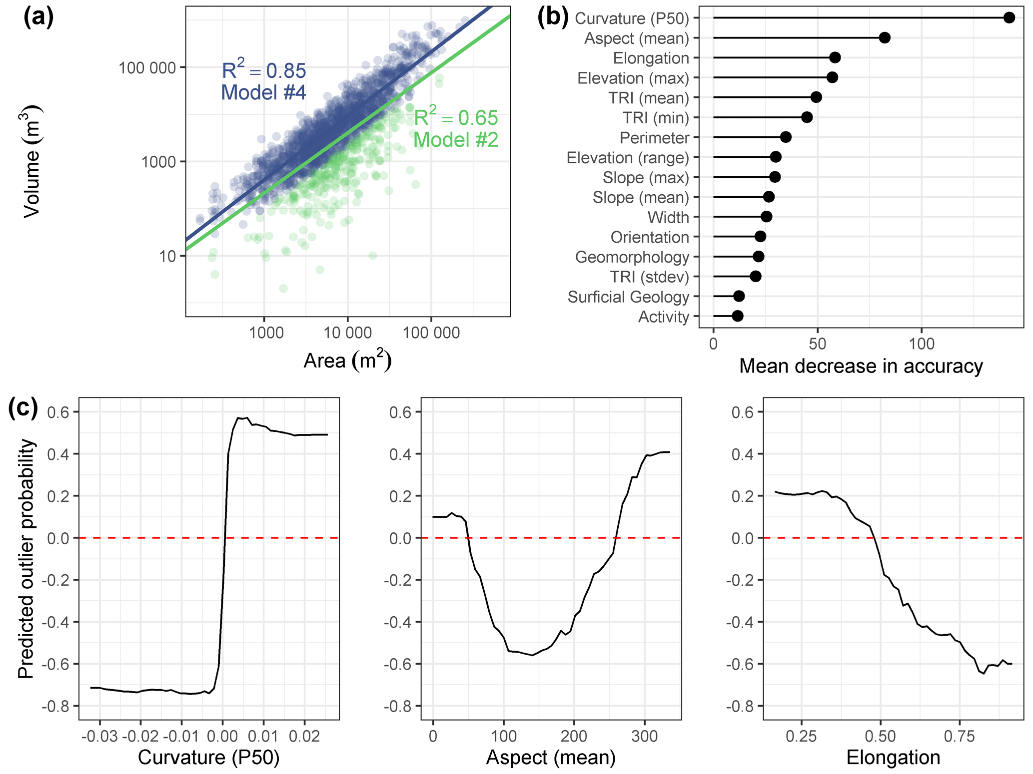
Figure 9Relationship between (a) slump area and slump fill volume. Scatterplot in (a) shows the regression models no. 2 and no. 4 (Table 3), as well as volumetric inliers (blue) and outliers (green), with observed model improvements when volumetric outliers were filtered out. (b) Variable importance in the random forest classification (predicting the probability of outliers) measured as the mean decrease in model accuracy scaled by the standard error of the change in model accuracy. (c) Partial dependence plots for the top three variables in order of importance: median profile curvature (50th percentile), mean aspect, and elongation ratio. The dashed red lines on the y axis in (c) indicate the point at which median curvature (> 0), mean aspect (less than 50∘ and greater than 270∘), and highly elongated slumps (e.g., < 0.5) were more likely to be classified as volumetric outliers.
The RF classification model to explore the morphological or environmental factors that discriminate between volumetric inliers (n= 1522) and outliers (n= 1139) indicated that median profile curvature, mean aspect, and elongation ratio were the top three predictors distinguishing the two groups (Fig. 9b). This binary classification model had an overall accuracy of 84 % (95 % CI: 80 to 87 %) and classified slumps as outliers and inliers with a user's accuracy of 82 % and 85 %, respectively. Partial dependence plots showed that disturbance areas characterized by a positive median profile curvature that were highly elongated – and for our study area, with a mean aspect ranging from 270∘ (west) to 50∘ (northeast) – were more likely to be classified as volumetric outliers (Fig. 9c). These characteristics were predominantly associated with slump-affected areas extending along shorelines in the APTC (Table 3), where wave erosion and shoreline retreat have driven long-term polycyclic activity (Kokelj et al., 2009; Ramage et al., 2017) and where active slumping often occurs within larger inactive shoreline scar areas digitized as a single polycyclic disturbance in the MSI (Figs. 2, 6b). The results highlight that the pre-disturbance surface interpolation, and therefore the estimation of volume, did not perform well, with disturbance areas that were elongated perpendicular to the local slope common to slope disturbances along eroding shorelines in the study region.
For the model including percent activity and data source, the removal of the volumetric outliers improved model fit from an adj-R2 of 0.66 to an adj-R2 of 0.86 (n= 1522; Table 3, model no. 3). An improved model fit of adj-R2 of 0.85 was also obtained for the simplest model between slump area and volume (model no. 4; Eq. 4). For the full model, percent activity was a significant secondary explanatory variable (p < 0.001), but data source (p= 0.354) was not. Both models had normally distributed residuals and no evidence of heteroscedasticity or influential samples.
Table 4Statistics of multiple linear regression models.
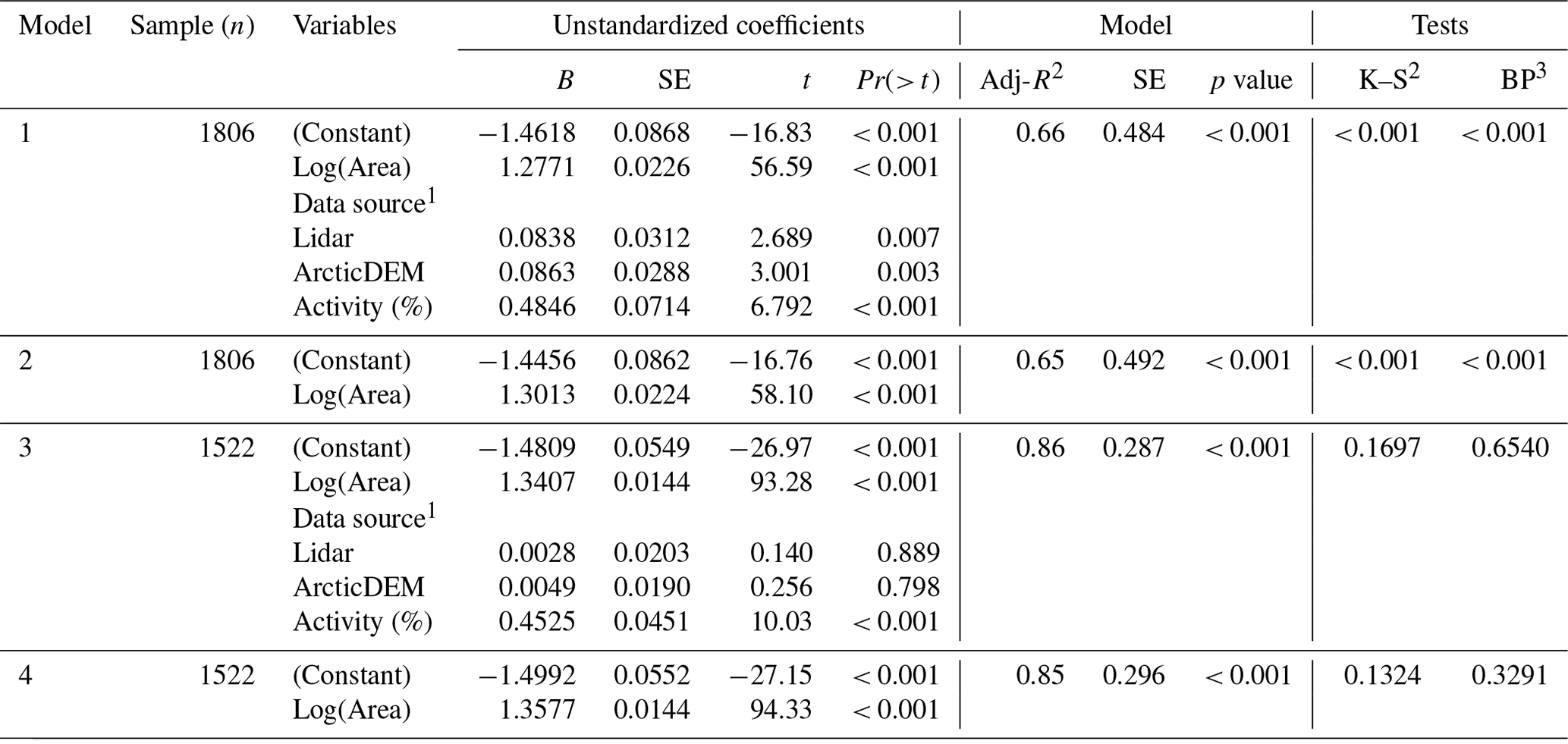
1 DEM data source: 2004 MVAP, 2011 lidar, or circa 2016 ArcticDEM; a categorical variable included to address temporal auto-correlation between multiple observations of the same slump across the DEM datasets and digitization periods. 2 Kolmogorov–Smirnov test for normality of residuals (p value). 3 Breusch–Pagan test for constant variance or heteroscedasticity (p value).
4.1 Pre-disturbance terrain methods
Thaw slumps are chronic, multi-year mass-wasting features, an important distinction from most landslides that are typically associated with a single triggering event, and the majority of scar volume represents a one-time translocation of mass on the landscape. For our thaw slump inventory, we are considering volume eroded since initiation, which could be on centennial timescales or greater. Obtaining the volume of a chronic erosion site can be challenging if the slump scar pre-dates regional topographic surveys. Utilizing data from fluvially incised ice-rich terrain (Kokelj et al., 2021), the approximation of pre-disturbance topography using natural neighbour (NN) interpolation achieved satisfactory results without complex parameterization (Fig. 4a). These findings compare well with other studies that identified NN elevation void-filling interpolation as the most appropriate technique, balancing accuracy and shape reliability across a range of natural environments (Bater and Coops, 2009; Boreggio et al., 2018). NN likely achieved the best results due to its simplicity and tendency to adapt to the structure of the elevation data by finding the closest subset of known elevation points to an unknown point and applying weights based on proportionate areas to interpolate a value. These results (Fig. 4) validate the choice of NN methodology implemented in Kokelj et al. (2021) and contribute a level of precision to the previously derived volumes, whereby known uncertainties (Fig. 5c) can now be applied in estimations of material mobilization from hillslopes (Tunnicliffe and Church, 2011) and in earth system models. Like Tseng et al. (2013), we determined error in absolute volume estimation to be less than 20 % for small features and less than 10 % for larger slope disturbances. The variability in volume estimates attributable to interpolation error decreases with increasing disturbance area, and there is an inverse association between slump area and relative volumetric error (Fig. 5c, d). For example, the total modelled volume of the 71 active thaw slump disturbances ( m3) from Kokelj et al. (2021) is associated with an interpolation-induced total volumetric uncertainty of m3 or about 8 % of estimated eroded volume. These volumetric uncertainties may be different depending on the accuracy and resolution of the source DEM, whereby the use of coarser-resolution DEMs (e.g., 10 or 30 m spatial resolution) will likely be associated with higher relative volumetric uncertainties. In the following sections we evaluate whether NN is a suitable interpolation approach across a broad range of RTS-affected terrains including more complex disturbance morphologies and different activity levels.
4.2 Multisource slump inventory (MSI)
Retrogressive thaw slumps are dynamic mass-wasting features that develop over periods of years to decades to millennia as thaw-driven processes and feedbacks interact with topography, ground ice and substrate conditions, and climate (Lacelle et al., 2010; Kokelj et al., 2015). Patterns in the distribution of slump-affected slopes and variation in the activity levels may be obfuscated due to the difficulties with the detection and delineation of active and stabilized slopes, limiting our understanding of the processes modifying the landscape and their spatial distribution. The analysis of MSI results demonstrate that retrogressive thaw slumps can be mapped and attributed consistently using a time composite of high-resolution hillshade DEMs supported by optical imagery (Figs. 2, 6). These procedures and a visual assessment of activity and field-based knowledge of thaw slump processes and forms can be implemented at a regional scale to inventory disturbances, detect previously unmapped disturbances, and track change through time (Fig. 6c). Precise manual measurement of surface area and a consistent characterization scheme were important in developing a multi-temporal spatial dataset to explore area–volume relationships (Van der Sluijs and Kokelj, 2023). The MSI concept does not negate other manual or semi-automated inventory initiatives (e.g., Segal et al., 2016; Huang et al., 2020; Nitze et al., 2021; Swanson, 2021; Runge et al., 2022); rather it contributes to knowledge of differences in slump ontology and detectability and provides a new approach on how to define and demarcate thaw slump disturbances. These methods and data enable us to explore scar characteristics and allometric properties, which has become possible as improved data resolution allows for greater topographic detail to be captured and visualized (Guzzetti et al., 2012; Clare et al., 2019).
The MSI dataset, summarized for the two study regions, indicates that about half of the thaw-slump-affected slopes were stable (Figs. 7, 8), that the vast majority of recent thaw slump activity can be associated with areas of past disturbance, and that there is significant morphometric diversity in the active and stable landforms. The MSI dataset reveals that between 40 % and 60 % of slump-affected slopes detected by this inventory were inactive disturbances. The median area of stable thaw slump disturbance is lower than for the population with varying activity levels in both study areas (Fig. 7; Table 3). The data also show that the total area of active thaw slumping has increased in APTC by 69 % between 2004 and 2016, yet the total disturbance area has remained the same because the majority of activity has occurred within old or ancient scar areas (Figs. 2c, 2d, 8). The increase in polycyclic activity is evacuating greater amounts of materials from within scar concavities, which has implications for the evolution of thawing slopes and area–volume relationships where thaw slump activity levels may account for scattering in area–volume models. There is growing evidence that contemporary slumps in PP and APTC are enlarging to the point that they are surpassing the extents of the historical disturbances from which they originated (Kokelj et al., 2015, 2021). The stabilized disturbance areas typically have higher ground temperatures and greater active layer thicknesses than undisturbed terrain, and they are situated in areas of ice-rich permafrost that predispose the surface for future thaw-driven instability (Figs. 2, 8) (Kokelj et al., 2009). Our observations indicate that contemporary and historical disturbances are closely linked, highlighting the need for inventory methods such as the MSI for their detection and monitoring. Additionally, the MSI observations may inspire additional satellite remote sensing avenues to detect these important landscape features over larger spatial extents.
These results also highlight the importance of distinguishing between process and form when mapping thaw-driven mass-wasting features. The delineation of slump-affected areas accomplished in the past through examining orthomosaics is less common now with the focus on thaw-driven change and utilizing planform, coarser-resolution remote sensing data with an emphasis on broad spatial coverage (Brooker et al., 2014; Lewkowicz and Way, 2019; Runge et al., 2022). The delineation of areas affected by a continuum of active, stable, and old thaw slump scars can produce a robust regional account of “slump-affected areas”, whereas inventories that map “active slumping” are implicitly documenting processes rather than forms. Mapping focused on change differs from approaches typically implemented in landslide mapping, where most features have occurred as the result of episodic events (Guzzetti et al., 2012). The distinction between active processes and forms is particularly important to consider when inventorying, mapping, and monitoring chronic slope failures such as retrogressive thaw slumping, where progressive growth and polycyclicity are inherent due to the underlying terrain conditions, the nature of the process, and positive feedbacks associated with disturbed permafrost terrain.
The MSI demonstrates that most geomorphically active disturbances are comprised of varying proportions of active and stabilized terrain, emphasizing the complex nature of polycyclic retrogressive thaw slumping. Utilizing high-resolution DEMs supported by optical imagery and methods implemented here also makes it possible to examine the relative levels of activity and the variation in morphometry of slump-affected terrain. For example, slumps in fluvially incised terrain of the PP had higher elongation ratios reflecting compact or rounded morphology that is more common to classic, cuspate-shaped thaw slumps (Fig. 7c; Table 3), with ratios increasing with activity level. In the APTC both classic cuspate features and elongated thaw slump disturbance occur, with the latter morphology typically characterizing eroding shorelines (Figs. 2b–e, 7b). The underlying DEMs required to generate the MSI data also enable topographic indices, such as terrain roughness, to be estimated. Descriptive statistics show that topographic roughness of slumps varied between the two study regions with increasing roughness in more highly active disturbances on PP. Together these analyses indicate variability in the morphology of RTS-affected slopes, leading to challenges in thaw slump detection, delineation, and determining scaling behaviour.
4.3 Area–volume relationships for thaw slumps
The interpolation methods and the MSI database enabled us to explore area–volume models for slumps of varying activity levels, spanning 6 orders of magnitude in volume and occurring across a wide range of geomorphic settings. The scaling coefficient for populations of inactive and active slumps (δ= 1.36±0.01) is positioned near the lower end of deep-seated bedrock landslides (δ= 1.3–1.6) and the higher end of soil landslides (δ= 1.1–1.4), and it exceeds submarine landslides (δ= 1.0–1.1), regardless of differences in failure properties (Chaytor et al., 2009; Larsen et al., 2010). The empirical evidence gathered in this study confirms that a population of disturbance areas consisting of ancient, recently active, and highly active slumps have a non-linear relationship with the volume (i.e., δ > ±1.0); however, due to the dynamics of slump evolution (Kokelj et al., 2015), the proportional erosion depth is heterogeneous. The scaling coefficient of inactive/old and active/modern slumps (δ= 1.36, n= 1522) observed in this study is lower than the δ= 1.42 obtained by Kokelj et al. (2021), which was based on active slumps (n= 71) with a “classic” cuspate or bowl-shaped form. These differences suggest that slump sub-populations grouped by terrain conditions, disturbance geometry, and activity levels may produce different scaling coefficients within and between geographic regions, warranting the investigation of increasing slump activity on morphometry.
This study also indicates that variation in the scaling factor δ can be expected due to differences in slump inventory approaches and guiding ontologies. Recently, Bernhard et al. (2022) determined a δ= 1.17 and δ= 1.27 for the Tuktoyaktuk Coastlands and Peel Plateau regions, respectively, based on differencing winter TanDEM-X DEMs and determining relationships between the “area showing an elevation decrease” and “the volume loss between measurement dates”. The differences in δ with our study bring attention to the problem of scar definition and DEM resolution, as small differences in δ lead to substantial variation in volume predictions (Fig. 1). For example, applying δ= 1.5 instead of δ= 1.4 produces a volume difference of a factor of 2 (Larsen et al., 2010; Tseng et al., 2013). Differences in δ may be attributed to data sources with coarser spatial resolution and greater vertical uncertainty, or it may be due to the temporal window of data acquisition, where differenced winter DEMs have a potential elevation bias due to incomplete radar penetration of snowdrifts or varying snow depths between years of observation. The δ reported by Bernhard et al. (2022) highlights a critical point of distinction between this study and Kokelj et al. (2021), as well as the larger body of landslide area–volume literature (Jaboyedoff et al., 2020), as scaling based on the total area and fill volume of a scar zone (i.e., fill volume scaling) is different from their model which is based on annual changes in surface area regressed against annual volumetric change (i.e., episodic volume scaling). Both approaches are valid for assessing the impacts of thaw slumping as they provide different means of understanding the environmental implications of slump enlargement. Models based on episodic or annual change may provide an annual yield from the thawing headwalls of active slumps during a periodic wave of activity. In contrast, estimating erosion depth from the full scar area is aimed at measuring the time-integrated changes to yield models that elucidate the longer-term trajectory of the slump-affected landscape, whereby concavities integrate erosion over decades to millennia. The method and ontological definition by which the process of slumping and active and inactive disturbance areas are inventoried and represented volumetrically are therefore important considerations that require clear definitions when scoping future studies.
Through mapping a broad range of slump-affected slopes, numerous volumetric outliers were detected where the modelling of pre-disturbance terrain (Fig. 5) did not fit the highly elongated (low elongation ratio) and convex slump topographies (e.g., Fig. 6b). These outliers are related to uncertainty in defining the pre-disturbed slope configuration, especially for coastal slumps or lacustrine slumps which typically exhibit narrow, elongated extents due to long-term shoreline retreat and complex interactions between simultaneous headwall retreat and wave-form erosion (Obu et al., 2016; Clark et al., 2021). Shoreline slumps along lakes typically initiate due to lateral talik expansion, thaw of ice-rich permafrost subjacent to the lakeshore, and lake-bottom subsidence (Kokelj et al., 2009), whereas in coastal settings rapid erosion of ice-rich shorelines driven by wave action produces dynamic conditions that extend beyond those associated with thaw slump development alone (Lantuit et al., 2012; Ramage et al., 2017; Leibman et al., 2021; Berry et al., 2021). Lake-bottom subsidence is effectively “invisible”, skewing volumetric estimates of yield. Attempts at inferring and repositioning ancient lake edges or former coast edges (e.g., Ramage et al., 2017) were not made in this study, nor were bathymetric data available to improve digitizations; hence estimates of many lacustrine/coastal slump volumes were underestimated to the point of not meeting the volumetric uncertainty threshold. The relationship between planimetric and volumetric erosion measurements for highly elongated slumps and coastal erosion sections can be complex (Obu et al., 2016), where improved prediction for shoreline slumps likely requires data on sub-surface conditions and knowledge of topographic profiles of undisturbed lake edges to parameterize interpolation algorithms. The challenges encountered with pre-disturbance terrain modelling are in part related to slump ontology, as well as a dichotomy between event-based mass wasting and chronic denudation of shoreline slumps where ice-rich topography is prone to progressive failure over long time periods and under seasonal climate forcing.
Retrogressive thaw slumps are multi-year, chronic disturbances that are increasingly important modifiers of ice-rich permafrost terrain. Quantifying geomorphic characteristics of thaw-driven landslides is required to understand their influence on landscape evolution, downstream sedimentary and geochemical effects, and the release or sequestration of organic carbon. In this research, our goal was to couple knowledge of thaw slump processes and forms with remote sensing tools to advance holistic approaches to monitoring and quantifying the geomorphic effects of retrogressive thaw slumps. We evaluated surface interpolation techniques to derive slump volumes based on DEM differencing (objective A), and we developed a high-resolution DEM-based slump inventory method to track surface area and activity levels (objective B). These methods were integrated to explore area–volume relationships for retrogressive thaw-slump-affected slopes (objective C). In summary, this study improved tools to estimate slump volume and calculate uncertainty arising from pre-disturbance terrain reconstructions. Natural neighbour interpolation achieved the best precision for modelled pre-disturbance topography. Error estimates in slump volume were < 10 % for large disturbances and less than 10 %–20 % for small to medium slumps.
A consistent method (MSI) for delineating slump-affected slopes and determining activity levels using high-resolution DEMs and optical imagery was developed. Significant variation in the morphology of slumps occurs in association with terrain type, geomorphic setting, and activity level. The MSI inventory documented widespread evidence of historical disturbances, most of which are currently inactive. The majority of active slumping is associated with areas of past disturbance, indicating that stable thaw slumps are an important indicator of sensitive terrain. This study corroborated past results indicating a significant (69 %) increase in active slumping between 2004–2016 for the APTC area.
The datasets generated in the first two sections of the paper enabled area–volume relationships of RTS-affected slopes to be explored. The resulting power-law model (adj-R2 of 0.85, n= 1522) enables a robust assessment of thaw-driven landslide impacts for regions where disturbance area is determined. In the analysis, outliers in the relationship were elongated coastal slump areas, providing constraints on model applications.
Future directions of research should involve revisiting thaw-driven landslide ontology to support scoping and informed interpretation of remote sensing outputs; exploring factors driving variation in slump morphometry and activity level; and determining whether area–volume relations vary between regions, among other thaw-driven disturbance types.
Datasets used in this publication and sources are summarized in Table 1. Slump delineations of the MSI are accessible via Van der Sluijs and Kokelj (2023, https://doi.org/10.46887/2023-013). Flowchart and geoprocessing steps for developing the input DEMs and the pre-disturbance terrain methods are available in the Supplement. Python code to derive slump volumes is described in Sect. S4 and available at https://github.com/jurjenvdsluijs/RTSareavolume (DEM_PredisturbanceGeneration_AreaVolumeCalc_Batch_NN_Py3.py; last access: 25 October 2023; https://doi.org/10.5281/zenodo.8357261, Van der Sluijs, 2023). Derived slump volumes are further described in Sect. S5 and available at https://github.com/jurjenvdsluijs/RTSareavolume (MSI_2022_10_Volumes_Outlierclass.csv; https://doi.org/10.5281/zenodo.8357261, Van der Sluijs, 2023).
The supplement related to this article is available online at: https://doi.org/10.5194/tc-17-4511-2023-supplement.
All authors developed the paper concept. JvdS and SVK contributed to field data collection and formulation of the multisource slump inventory concept and implementation. JvdS processed the geospatial datasets and developed and interpreted statistical analyses with guidance from SVK and JFT. JvdS drafted and revised the paper and figures with input from all authors.
The contact author has declared that none of the authors has any competing interests.
Publisher’s note: Copernicus Publications remains neutral with regard to jurisdictional claims in published maps and institutional affiliations.
This work is part of a long-term permafrost monitoring and research program within the Government of Northwest Territories (GNWT) and NWT Geological Survey with partners including the NWT Centre for Geomatics. We are grateful to the Indigenous peoples of the Gwich'in Settlement Area and Inuvialuit Settlement Region of the Northwest Territories for the opportunity to work collaboratively and to learn and gather knowledge on their lands. Long-term support from the Tetl'it and Ehdiitat Renewable Resource Councils, the Inuvik and Tuktoyaktuk Hunters and Trappers Committees, the Inuvialuit Joint Secretariat, the Inuvialuit Land Administration, the Inuvialuit Regional Corporation (Charles Klengenberg), and the Aurora Research Institute (Joel McAlister) is gratefully acknowledged. Field support from Christine Firth, Andrew Koe, Eugene Pascale, Ashley Rudy, Steven Tetlitchi, Alice Wilson, and Billy Wilson and is also sincerely acknowledged. William Woodley (NWT Centre for Geomatics) processed MVAP contour lines into the 3 m DEM.
This research has been supported by the Department of Environment and Natural Resources Climate Change and the Northwest Territories Cumulative Impact Monitoring Program of the GNWT (grant nos. 164 and 186, Steven V. Kokelj); the Natural Science and Engineering Research Council of Canada; and the Polar Continental Shelf Program, Natural Resources Canada (projects 313-18, 316-19, 318-20, and 320-20 to Steven V. Kokelj).
This paper was edited by Christian Beer and reviewed by Matthias Siewert and one anonymous referee.
Aylsworth, J. M., Rodkin-Duk, A., Robertson, T., and Traynor, J. A.: Landslide of the Mackenzie valley and adjacent mountanainous and coastal regions, in: The Physical Environment of the Mackenzie Valley: A Baseline for the Assessment of Environmental Change, edited by: Dyke, L. D. and Brooks, G. R., 167–176, ISBN 0-660-18281-5, 2000.
Bater, C. W. and Coops, N. C.: Evaluating error associated with lidar-derived DEM interpolation, Comput. Geosci., 35, 289–300, https://doi.org/10.1016/j.cageo.2008.09.001, 2009.
Bergonse, R. and Reis, E.: Reconstructing pre-erosion topography using spatial interpolation techniques: A validation-based approach, J. Geogr. Sci., 25, 196–210, https://doi.org/10.1007/s11442-015-1162-2, 2015.
Bernhard, P., Zwieback, S., Leinss, S., and Hajnsek, I.: Mapping Retrogressive Thaw Slumps Using Single-Pass TanDEM-X Observations, IEEE J. Sel. Top. Appl., 13, 3263–3280, https://doi.org/10.1109/JSTARS.2020.3000648, 2020.
Bernhard, P., Zwieback, S., Bergner, N., and Hajnsek, I.: Assessing volumetric change distributions and scaling relations of retrogressive thaw slumps across the Arctic, The Cryosphere, 16, 1–15, https://doi.org/10.5194/tc-16-1-2022, 2022.
Berry, H. B., Whalen, D., and Lim, M.: Long-term ice-rich permafrost coast sensitivity to air temperatures and storm influence: lessons from Pullen Island, Northwest Territories, Canada, Arctic Science, 7, 723–745, https://doi.org/10.1139/as-2020-0003, 2021.
Boreggio, M., Bernard, M., and Gregoretti, C.: Evaluating the Differences of Gridding Techniques for Digital Elevation Models Generation and Their Influence on the Modeling of Stony Debris Flows Routing: A Case Study From Rovina di Cancia Basin (North-Eastern Italian Alps), Front. Earth Sci., 6, 89, https://doi.org/10.3389/feart.2018.00089, 2018.
Brardinoni, F., Slaymaker, O., and Hassan, M. A.: Landslide inventory in a rugged forested watershed: a comparison between air-photo and field survey data, Geomorphology, 54, 179–196, https://doi.org/10.1016/S0169-555X(02)00355-0, 2003.
Breiman, L.: Random Forests, Mach. Learn., 45, 5–32, https://doi.org/10.1023/a:1010933404324, 2001.
Brooker, A., Fraser, R. H., Olthof, I., Kokelj, S. V., and Lacelle, D.: Mapping the activity and evolution of retrogressive thaw slumps by tasselled cap trend analysis of a Landsat satellite image stack, Permafrost Periglac., 25, 243–256, https://doi.org/10.1002/ppp.1819, 2014.
Burn, C. R.: Cryostratigraphy, paleogeography, and climate change during the early Holocene warm interval, western Arctic coast, Canada, Can. J. Earth Sci., 34, 912–925, https://doi.org/10.1139/e17-076, 1997.
Burn, C. R.: The thermal regime of a retrogressive thaw slump near Mayo, Yukon Territory, Can. J. Earth Sci., 37, 967–981, https://doi.org/10.1139/e00-017, 2000.
Burn, C. R. and Friele, P. A.: Geomorphology, Vegetation Succession, Soil Characteristics and Permafrost in Retrogressive Thaw Slumps near Mayo, Yukon Territory, Arctic, 42, 31–40, 1989.
Burn, C. R. and Kokelj, S. V.: The environment and permafrost of the Mackenzie Delta area, Permafrost Periglac., 20, 83–105, https://doi.org/10.1002/ppp.655, 2009.
Burn, C. R. and Lewkowicz, A. G.: Canadian landform examples - 17 retrogressive thaw slumps, Can. Geogr./Geogr. Can., 34, 273–276, https://doi.org/10.1111/j.1541-0064.1990.tb01092.x, 1990.
Campbell, D. and Church, M.: Reconnaissance sediment budgets for Lynn Valley, British Columbia: Holocene and contemporary time scales, Can. J. Earth Sci., 40, 701–713, https://doi.org/10.1139/e03-012, 2003.
Chaytor, J. D., ten Brink, U. S., Solow, A. R., and Andrews, B. D.: Size distribution of submarine landslides along the U.S. Atlantic margin, Mar. Geol., 264, 16–27, https://doi.org/10.1016/j.margeo.2008.08.007, 2009.
Clare, M., Chaytor, J., Dabson, O., Gamboa, D., Georgiopoulou, A., Eady, H., Hunt, J., Jackson, C., Katz, O., Krastel, S., León, R., Micallef, A., Moernaut, J., Moriconi, R., Moscardelli, L., Mueller, C., Normandeau, A., Patacci, M., Steventon, M., Urlaub, M., Völker, D., Wood, L., and Jobe, Z.: A consistent global approach for the morphometric characterization of subaqueous landslides, Geological Society, London, Special Publications, 477, 455–477, https://doi.org/10.1144/SP477.15, 2019.
Clark, A., Moorman, B., Whalen, D., and Fraser, P.: Arctic coastal erosion: UAV-SfM data collection strategies for planimetric and volumetric measurements, Arctic Science, 7, 605–633, https://doi.org/10.1139/as-2020-0021, 2021.
Côté, M. M., Duchesne, C., Wright, J., and Ednie, M.: Digital compilation of the surficial sediments of the Mackenzie Valley corridor, Yukon Coastal Plain, and the Tuktoyaktuk Peninsula, Natural Resources Canada, Geological Survey of Canada, Open File 7289, 38 pp., https://doi.org/10.4095/292494, 2013.
Fraser, R. H., Olthof, I., Kokelj, S. V., Lantz, T. C., Lacelle, D., Brooker, A., Wolfe, S., and Schwarz, S.: Detecting landscape changes in high latitude environments using Landsat trend analysis: 1. visualization, Remote Sensing, 6, 11533–11557, https://doi.org/10.3390/rs61111533, 2014.
Gudowicz, J. and Paluszkiewicz, R.: MAT: GIS-Based Morphometry Assessment Tools for Concave Landforms, Remote Sensing, 13, 2810, https://doi.org/10.3390/rs13142810, 2021.
Guzzetti, F., Mondini, A. C., Cardinali, M., Fiorucci, F., Santangelo, M., and Chang, K.-T.: Landslide inventory maps: New tools for an old problem, Earth-Sci. Rev., 112, 42–66, https://doi.org/10.1016/j.earscirev.2012.02.001, 2012.
Huang, L., Luo, J., Lin, Z., Niu, F., and Liu, L.: Using deep learning to map retrogressive thaw slumps in the Beiluhe region (Tibetan Plateau) from CubeSat images, Remote Sens. Environ., 237, 111534, https://doi.org/10.1016/j.rse.2019.111534, 2020.
Huang, L., Lantz, T. C., Fraser, R. H., Tiampo, K. F., Willis, M. J., and Schaefer, K.: Accuracy, Efficiency, and Transferability of a Deep Learning Model for Mapping Retrogressive Thaw Slumps across the Canadian Arctic, Remote Sensing, 14, 2747, https://doi.org/10.3390/rs14122747, 2022.
Jaboyedoff, M., Carrea, D., Derron, M.-H., Oppikofer, T., Penna, I. M., and Rudaz, B.: A review of methods used to estimate initial landslide failure surface depths and volumes, Eng. Geol., 267, 105478, https://doi.org/10.1016/j.enggeo.2020.105478, 2020.
Klar, A., Aharonov, E., Kalderon-Asael, B., and Katz, O.: Analytical and observational relations between landslide volume and surface area, J. Geophys. Res.-Earth, 116, F02001, https://doi.org/10.1029/2009JF001604, 2011.
Kokelj, S. V., Jenkins, R. E., Milburn, D., Burn, C. R., and Snow, N.: The influence of thermokarst disturbance on the water quality of small upland lakes, Mackenzie Delta region, Northwest Territories, Canada, Permafrost Periglac., 16, 343–353, https://doi.org/10.1002/ppp.536, 2005.
Kokelj, S. V., Lantz, T. C., Kanigan, J., Smith, S. L., and Coutts, R.: Origin and polycyclic behaviour of tundra thaw slumps, Mackenzie Delta region, Northwest Territories, Canada, Permafrost Periglac., 20, 173–184, https://doi.org/10.1002/ppp.642, 2009.
Kokelj, S. V., Lacelle, D., Lantz, T. C., Tunnicliffe, J., Malone, L., Clark, I. D., and Chin, K. S.: Thawing of massive ground ice in mega slumps drives increases in stream sediment and solute flux across a range of watershed scales, J. Geophys. Res.-Earth, 118, 681–692, https://doi.org/10.1002/jgrf.20063, 2013.
Kokelj, S. V., Lantz, T. C., Wolfe, S. A., Kanigan, J. C., Morse, P. D., Coutts, R., Molina-Giraldo, N., and Burn, C. R.: Distribution and activity of ice wedges across the forest-tundra transition, western Arctic Canada, J. Geophys. Res.-Earth, 119, 2032–2047, https://doi.org/10.1002/2014JF003085, 2014.
Kokelj, S. V., Tunnicliffe, J., Lacelle, D., Lantz, T. C., Chin, K. S., and Fraser, R.: Increased precipitation drives mega slump development and destabilization of ice-rich permafrost terrain, northwestern Canada, Global Planet. Change, 129, 56–68, https://doi.org/10.1016/j.gloplacha.2015.02.008, 2015.
Kokelj, S. V., Lantz, T. C., Tunnicliffe, J., Segal, R., and Lacelle, D.: Climate-driven thaw of permafrost preserved glacial landscapes, northwestern Canada, Geology, 45, 371–374, https://doi.org/10.1130/g38626.1, 2017a.
Kokelj, S. V., Tunnicliffe, J. F., and Lacelle, D.: The Peel Plateau of northwestern Canada: an ice-rich hummocky moraine landscape in transition, in: Landscapes and Landforms of Western Canada, edited by: Slaymaker, O., Springer International Publishing, Cham, Switzerland, 109–122, ISBN 978-3-319-44593-9, https://doi.org/10.1007/978-3-319-44595-3, 2017b.
Kokelj, S. V., Kokoszka, J., van der Sluijs, J., Rudy, A. C. A., Tunnicliffe, J., Shakil, S., Tank, S. E., and Zolkos, S.: Thaw-driven mass wasting couples slopes with downstream systems, and effects propagate through Arctic drainage networks, The Cryosphere, 15, 3059–3081, https://doi.org/10.5194/tc-15-3059-2021, 2021.
Lacelle, D., Bjornson, J., and Lauriol, B.: Climatic and geomorphic factors affecting contemporary (1950–2004) activity of retrogressive thaw slumps on the Aklavik Plateau, Richardson Mountains, NWT, Canada, Permafrost Periglac., 21, 1–15, https://doi.org/10.1002/ppp.666, 2010.
Lacelle, D., Brooker, A., Fraser, R. H., and Kokelj, S. V.: Distribution and growth of thaw slumps in the Richardson Mountains–Peel Plateau region, northwestern Canada, Geomorphology, 235, 40–51, https://doi.org/10.1016/j.geomorph.2015.01.024, 2015.
Lacelle, D., Fontaine, M., Pellerin, A., Kokelj, S. V., and Clark, I. D.: Legacy of Holocene Landscape Changes on Soil Biogeochemistry: A Perspective From Paleo-Active Layers in Northwestern Canada, J. Geophys. Res.-Biogeo., 124, 2662–2679, https://doi.org/10.1029/2018JG004916, 2019.
Lantuit, H. and Pollard, W. H.: Fifty years of coastal erosion and retrogressive thaw slump activity on Herschel Island, southern Beaufort Sea, Yukon Territory, Canada, Geomorphology, 95, 84–102, https://doi.org/10.1016/j.geomorph.2006.07.040, 2008.
Lantuit, H., Pollard, W. H., Couture, N., Fritz, M., Schirrmeister, L., Meyer, H., and Hubberten, H.-W.: Modern and Late Holocene Retrogressive Thaw Slump Activity on the Yukon Coastal Plain and Herschel Island, Yukon Territory, Canada, Permafrost Periglac., 23, 39–51, https://doi.org/10.1002/ppp.1731, 2012.
Lantz, T. C. and Kokelj, S. V.: Increasing rates of retrogressive thaw slump activity in the Mackenzie Delta region, N.W.T., Canada, Geophys. Res. Lett., 35, L06502, https://doi.org/10.1029/2007GL032433, 2008.
Lantz, T. C., Kokelj, S. V., Gergel, S. E., and Henry, G. H. R.: Relative impacts of disturbance and temperature: persistent changes in microenvironment and vegetation in retrogressive thaw slumps, Glob. Change Biol., 15, 1664–1675, https://doi.org/10.1111/j.1365-2486.2009.01917.x, 2009.
Larsen, I. J., Montgomery, D. R., and Korup, O.: Landslide erosion controlled by hillslope material, Nat. Geosci., 3, 247–251, https://doi.org/10.1038/ngeo776, 2010.
Leibman, M., Kizyakov, A., Zhdanova, Y., Sonyushkin, A., and Zimin, M.: Coastal Retreat Due to Thermodenudation on the Yugorsky Peninsula, Russia during the Last Decade, Update since 2001–2010, Remote Sensing, 13, 4042, https://doi.org/10.3390/rs13204042, 2021.
Lewkowicz, A. G.: Headwall retreat of ground-ice slumps, Banks Island, Northwest Territories, Can. J. Earth Sci., 24, 1077–1085, https://doi.org/10.1139/e87-105, 1987.
Lewkowicz, A. G. and Way, R. G.: Extremes of summer climate trigger thousands of thermokarst landslides in a High Arctic environment, Nat. Commun., 10, 1329, https://doi.org/10.1038/s41467-019-09314-7, 2019.
Luo, J., Niu, F., Lin, Z., Liu, M., and Yin, G.: Recent acceleration of thaw slumping in permafrost terrain of Qinghai-Tibet Plateau: An example from the Beiluhe Region, Geomorphology, 341, 79–85, https://doi.org/10.1016/j.geomorph.2019.05.020, 2019.
Mackay, J. R.: Segregated epigenetic ice and slumps in permafrost Mackenzie Delta area, N.W.T., Geographical Bulletin, 8, 59–80, 1966.
Mackay, J. R.: Some observations on the growth and deformation of epigenetic, syngenetic and anti-syngenetic ice wedges, Permafrost Periglac., 1, 15–29, https://doi.org/10.1002/ppp.3430010104, 1990.
Murton, J. B.: Ground-ice stratigraphy and formation at North Head, Tuktoyaktuk Coastlands, western Arctic Canada: a product of glacier–permafrost interactions, Permafrost Periglac., 16, 31–50, https://doi.org/10.1002/ppp.513, 2005.
Nitze, I., Heidler, K., Barth, S., and Grosse, G.: Developing and Testing a Deep Learning Approach for Mapping Retrogressive Thaw Slumps, Remote Sensing, 13, 4294, https://doi.org/10.3390/rs13214294, 2021.
Obu, J., Lantuit, H., Fritz, M., Pollard, W. H., Sachs, T., and Günther, F.: Relation between planimetric and volumetric measurements of permafrost coast erosion: a case study from Herschel Island, western Canadian Arctic, Polar Res., 35, 30313, https://doi.org/10.3402/polar.v35.30313, 2016.
Oguchi, T.: Drainage Density and Relative Relief in Humid Steep Mountains with Frequent Slope Failure, Earth Surf. Proc. Land., 22, 107–120, https://doi.org/10.1002/(SICI)1096-9837(199702)22:2<107::AID-ESP680>3.0.CO;2-U, 1997.
Porter, C., Morin, P., Howat, I., Noh, M.-J., Bates, B., Peterman, K., Keesey, S., Schlenk, M., Gardiner, J., Tomko, K., Willis, M., Kelleher, C., Cloutier, M., Husby, E., Foga, S., Nakamura, H., Platson, M., Wethington, M., Williamson, C., Bauer, G., Enos, J., Arnold, G., Kramer, W., Becker, P., Doshi, A., D'Souza, C., Cummens, P., Laurier, F., and Bojesen, M.: ArcticDEM, Version 3, Harvard Dataverse [data set], V1, https://doi.org/10.7910/DVN/OHHUKH, 2018.
Ramage, J. L., Irrgang, A. M., Herzschuh, U., Morgenstern, A., Couture, N., and Lantuit, H.: Terrain controls on the occurrence of coastal retrogressive thaw slumps along the Yukon Coast, Canada, J. Geophys. Res.-Earth, 122, 1619–1634, https://doi.org/10.1002/2017JF004231, 2017.
Rampton, V. N.: Quaternary Geology of the Tuktoyaktuk Coastlands, Northwest Territories., Geological Survey of Canada, Memoir 423, Ottawa, ON, Canada, https://doi.org/10.4095/126937, 1988.
Reuter, H. I., Nelson, A., and Jarvis, A.: An evaluation of void-filling interpolation methods for SRTM data, Int. J. Geogr. Inf. Sci., 21, 983–1008, https://doi.org/10.1080/13658810601169899, 2007.
Riley, S., Degloria, S., and Elliot, S. D.: A Terrain Ruggedness Index that Quantifies Topographic Heterogeneity, Int. J. Sci., 5, 23–27, 1999.
Runge, A., Nitze, I., and Grosse, G.: Remote sensing annual dynamics of rapid permafrost thaw disturbances with LandTrendr, Remote Sens. Environ., 268, 112752, https://doi.org/10.1016/j.rse.2021.112752, 2022.
Segal, R. A., Lantz, T. C., and Kokelj, S. V.: Acceleration of thaw slump activity in glaciated landscapes of the Western Canadian Arctic, Environ. Res. Lett., 11, 034025, https://doi.org/10.1088/1748-9326/11/3/034025, 2016.
Sladen, W. E., Parker, R. J. H., Kokelj, S. V., and Morse, P. D.: Geomorphologic feature mapping methodology developed for the Dempster Highway and Inuvik to Tuktoyaktuk Highway corridors, Geological Survey of Canada, Open File 8751, 56 pp., https://doi.org/10.4095/328181, 2021.
Smith, I. R. and Duong, L.: An assessment of surficial geology, massive ice, and ground ice, Tuktoyaktuk Peninsula, Northwest Territories: application to the proposed Inuvik to Tuktoyaktuk all-weather highway, Natural Resources Canada, Geological Survey of Canada, Open File 7106, 42 pp., https://doi.org/10.4095/292017, 2012.
Stark, C. P. and Hovius, N.: The characterization of landslide size distributions, Geophys. Res. Lett., 28, 1091–1094, https://doi.org/10.1029/2000GL008527, 2001.
Swanson, D. and Nolan, M.: Growth of retrogressive thaw slumps in the Noatak Valley, Alaska, 2010–2016, measured by airborne photogrammetry, Remote Sensing, 10, 983, https://doi.org/10.3390/rs10070983, 2018.
Swanson, D. K.: Permafrost thaw-related slope failures in Alaska's Arctic National Parks, c. 1980–2019, Permafrost Periglac., 32, 392–406, https://doi.org/10.1002/ppp.2098, 2021.
ten Brink, U. S., Geist, E. L., and Andrews, B. D.: Size distribution of submarine landslides and its implication to tsunami hazard in Puerto Rico, Geophys. Res. Lett., 33, L11307, https://doi.org/10.1029/2006GL026125, 2006.
Treharne, R., Rogers, B. M., Gasser, T., MacDonald, E., and Natali, S.: Identifying Barriers to Estimating Carbon Release From Interacting Feedbacks in a Warming Arctic, Frontiers in Climate, 3, 716464, https://doi.org/10.3389/fclim.2021.716464, 2022.
Tseng, C.-M., Lin, C.-W., Stark, C. P., Liu, J.-K., Fei, L.-Y., and Hsieh, Y.-C.: Application of a multi-temporal, LiDAR-derived, digital terrain model in a landslide-volume estimation, Earth Surf. Proc. Land., 38, 1587–1601, https://doi.org/10.1002/esp.3454, 2013.
Tunnicliffe, J. F. and Church, M.: Scale variation of post-glacial sediment yield in Chilliwack Valley, British Columbia, Earth Surf. Proc. Land., 36, 229–243, https://doi.org/10.1002/esp.2093, 2011.
Turner, K. W., Pearce, M. D., and Hughes, D. D.: Detailed Characterization and Monitoring of a Retrogressive Thaw Slump from Remotely Piloted Aircraft Systems and Identifying Associated Influence on Carbon and Nitrogen Export, Remote Sensing, 13, 171, https://doi.org/10.3390/rs13020171, 2021.
Van der Sluijs, J.: Supplementary code and data to Allometric scaling of retrogressive thaw slumps, Zenodo [code] and [data set], https://doi.org/10.5281/zenodo.8357261, 2023.
Van der Sluijs, J. and Kokelj, S. V.: High-resolution inventory of retrogressive thaw slump affected slopes using high spatial resolution Digital Elevation models and imagery, Peel Plateau and Anderson Plain – Tuktoyaktuk Coastlands, Northwest Territories, Northwest Territories Geological Survey [data set], https://doi.org/10.46887/2023-013, 2023.
Van der Sluijs, J., Kokelj, S. V., Fraser, R. H., Tunnicliffe, J., and Lacelle, D.: Permafrost Terrain Dynamics and Infrastructure Impacts Revealed by UAV Photogrammetry and Thermal Imaging, Remote Sensing, 10, 1734, https://doi.org/10.3390/rs10111734, 2018.
Ward Jones, M. K. and Pollard, W. H.: Daily Field Observations of Retrogressive Thaw Slump Dynamics in the Canadian High Arctic, ARCTIC, 74, 339–354, https://doi.org/10.14430/arctic73377, 2021.
Ward Jones, M. K., Pollard, W. H., and Jones, B. M.: Rapid initialization of retrogressive thaw slumps in the Canadian high Arctic and their response to climate and terrain factors, Environ. Res. Lett., 14, 055006, https://doi.org/10.1088/1748-9326/ab12fd, 2019.
Xia, Z., Huang, L., Fan, C., Jia, S., Lin, Z., Liu, L., Luo, J., Niu, F., and Zhang, T.: Retrogressive thaw slumps along the Qinghai–Tibet Engineering Corridor: a comprehensive inventory and their distribution characteristics, Earth Syst. Sci. Data, 14, 3875–3887, https://doi.org/10.5194/essd-14-3875-2022, 2022.
Zwieback, S., Kokelj, S. V., Günther, F., Boike, J., Grosse, G., and Hajnsek, I.: Sub-seasonal thaw slump mass wasting is not consistently energy limited at the landscape scale, The Cryosphere, 12, 549–564, https://doi.org/10.5194/tc-12-549-2018, 2018.