the Creative Commons Attribution 4.0 License.
the Creative Commons Attribution 4.0 License.
 | 26 Oct 2023
Local analytical optimal nudging for assimilating AMSR2 sea ice concentration in a high-resolution pan-Arctic coupled ocean (HYCOM 2.2.98) and sea ice (CICE 5.1.2) model
Alfatih Ali
Caixin Wang
Local analytical optimal nudging (LAON) is introduced and thoroughly evaluated for assimilating the Advanced Microwave Scanning Radiometer 2 (AMSR2) sea ice concentration (SIC) in the Norwegian High-resolution pan-Arctic ocean and sea ice Prediction System (NorHAPS). NorHAPS is a developing high-resolution (3–5 km) pan-Arctic coupled ocean and sea ice modeling and prediction system based on the HYbrid Coordinate Ocean Model (HYCOM version 2.2.98) and the Los Alamos multi-category sea ice model (CICE version 5.1.2), with the LAON for data assimilation. In this study, our focus is on the LAON assimilation of AMSR2 SIC, which is designed to update the model SIC in every time step such that the analysis will eventually reach the optimal estimate. The SIC innovation (observation minus model) is designed to be proportionally distributed to the multiple sea ice categories.
A hindcast experiment is performed with and without the LAON assimilation for the period 1 January 2021 to 30 April 2022, in which the extra computational cost for the LAON assimilation is about 5 % of the free run without assimilation. The results show that the LAON assimilation greatly improves the simulated sea ice concentration, extent, area, thickness, and volume, as well as the sea surface temperature (SST). It also produces significantly more accurate sea ice edge and marginal zone (MIZ) than the observed AMSR2 SIC that is assimilated when evaluated against the Norwegian Ice Service (NIS) ice chart. The results are also compared with the Copernicus Marine Environment Monitoring Service (CMEMS) operational SIC analyses from NEMO, TOPAZ4, and neXtSIM, which use ensemble Kalman filters and direct insertion for data assimilation. It is shown that the LAON assimilation produces significantly lower integrated ice edge error (IIEE) and integrated MIZ error (IME) than the CMEMS SIC analyses when evaluated against the NIS ice chart. LAON also produces a continuous and smooth evolution of sub-daily SIC, which avoids abrupt jumps often seen in other assimilated products. This efficient and accurate method is promising for data assimilation in global and high-resolution models.
- Article
(10808 KB) - Full-text XML
- BibTeX
- EndNote


Arctic sea ice is one of the most sensitive components in Earth's climate system. In recent decades it has been undergoing a dramatic change, where vast areas previously covered by multiyear sea ice are now dominated by younger, thinner ice or are even seasonally ice-free (Comiso, 2012; Meier et al., 2014; Kwok, 2018; Stroeve and Notz, 2018; Kacimi and Kwok, 2022; Constable et al., 2022; Sumata et al., 2023). While this change is opening new opportunities for accessing the Arctic (Smith and Stepheson, 2013; PAME, 2020; Berkman et al., 2022; Constable et al., 2022), it also brings higher environmental risks and climate challenges to the Arctic (Emmerson and Lahn, 2012; Meier et al., 2014; Dammann et al., 2018; Cohen et al., 2020). To effectively manage the opportunities and risks, sound measures are urgently needed to ensure adequate sustainable development, safe operation, and ecosystem-based management. Accurate and timely sea ice forecast is thus becoming more and more important for the planning and regulation of the activities in the Arctic (Eicken, 2013; Jung et al., 2016).
Accurate sea ice forecast depends strongly on the initial conditions, which are commonly prepared by data assimilation via a combination of model simulations and observations. A variety of sea ice data assimilation methods have been developed in the last 2 decades, including direct insertion (Caya et al., 2010; Posey et al., 2015; Williams et al., 2021), nudging (Lindsay and Zhang, 2006; Caya et al., 2010; Wang et al., 2013; Tietsche et al., 2013; Fritzner et al., 2018), optimal interpolation (OI; Zhang et al., 2003; Stark et al., 2008; Wang et al., 2013), three-dimensional variational assimilation (3D-Var; Caya et al., 2010; Buehner et al., 2013; Blockley et al., 2014; Waters et al., 2015), and the ensemble Kalman filter (EnKF; Lisæter et al., 2003; Sakov et al., 2012; Mathiot et al., 2012; Yang et al., 2014; Fritzner et al., 2018). It is noteworthy that when assimilating the same sea ice observations, the forecast quality tends to be quite similar regardless of the different assimilation methods (e.g., Caya et al., 2010; Fritzner et al., 2018).
In recent years, with the continuous development of coupled atmosphere, ocean, and sea ice models and increasing model spatial resolutions, there is a growing interest in computationally efficient data assimilation methods for providing accurate and timely high-resolution forecasts. In the present study, local analytical optimal nudging (LAON) is introduced to provide an efficient and accurate method to assimilate the high-resolution (3.125 km) Advanced Microwave Scanning Radiometer 2 (AMSR2) sea ice concentration (SIC) into the multi-category Los Alamos sea ice model CICE (Hunke et al., 2015) in the coupled ocean and sea ice model HYCOM–CICE. The extra computational cost for the LAON assimilation is negligibly small at about 5 % of the free run in the present study.
LAON is a further development of combined optimal interpolation and nudging (COIN; Wang et al., 2013). The originally empirical treatments of the combination of OI and nudging in COIN have been upgraded as a theoretically self-contained optimization (see Sect. 2). The analysis in LAON is designed to be gradually nudged to the optimal estimate rather than nudged toward the observation in the ordinary nudging (Anthes, 1974). The LAON assimilation is only performed forward in time, with the optimal nudging coefficient deduced analytically. This is different from variational optimal nudging (Zou et al., 1992; Vidard et al., 2003), where the optimal nudging coefficient is obtained through parameter estimation with a complex minimization procedure using integrations of both direct and adjoint models.
The present study is organized as follows. Section 2 introduces the coupled HYCOM–CICE model system, together with LAON that is coded in the multi-category CICE model for SIC data assimilation. In Sect. 3, a variety of observation data are introduced for model evaluation, including SIC, sea ice thickness (SIT), sea surface temperature (SST), and sea surface salinity (SSS), together with three Copernicus Marine Environment Monitoring Service (CMEMS) SIC analyses (NEMO, TOPAZ4, and neXtSIM). In Sect. 4 we perform a hindcast experiment with and without the LAON assimilation and evaluate the effect of the LAON SIC assimilation on the modeled ocean and sea ice variables. In Sect. 5 we further compare the LAON simulation with the CMEMS SIC analyses from the NEMO, TOPAZ4, and neXtSIM models and evaluate their skills in simulating sea ice edge and marginal ice zone (MIZ) against the Norwegian Ice Service (NIS) ice charts. In Sect. 6, we discuss some general issues relating to the data assimilation and model evaluation. The conclusions are given in Sect. 7.
The Norwegian High-resolution pan-Arctic ocean and sea ice Prediction System (NorHAPS) is a developing modeling and prediction system at the Norwegian Meteorological Institute. It is based on the coupled HYCOM–CICE model developed at the Nansen Environment and Remote Sensing Center (NERSC; https://github.com/nansencenter/NERSC-HYCOM-CICE, last access: 2021), with LAON for data assimilation. Its free run version (no data assimilation) is currently run operationally and delivers daily 10 d forecasts of sea surface height and sea surface velocity components to CMEMS as snapshots at 15 min frequency (Ali et al., 2021), which is available for free download from CMEMS (https://doi.org/10.48670/moi-00005, Copernicus Marine Service, 2019).
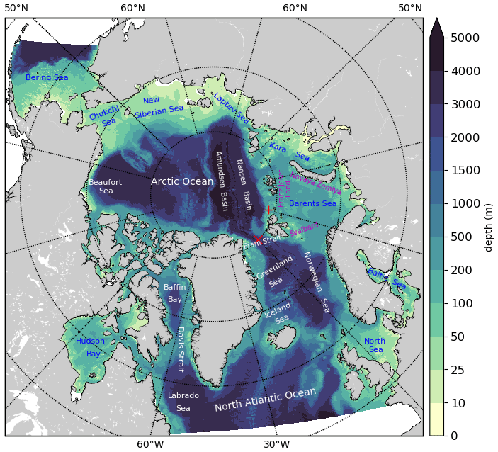
Figure 1Model domain and bathymetry of the coupled HYCOM–CICE model. The ocean and sea names are denoted using blue and white, which is only for clarity purposes. The red “+” and “x” show two point locations for comparison of hourly sea ice concentration in Fig. 12.
2.1 HYCOM–CICE model
The coupled HYCOM–CICE model is based on the HYbrid Coordinate Ocean Model (HYCOM version 2.2.98; Bleck, 2002) and the Los Alamos Community Ice Code (CICE version 5.1.2; Hunke et al., 2015). Their coupling is accomplished using the Earth System Modeling Framework (ESMF version 8.0). The model domain covers the Arctic and North Atlantic oceans and their marginal seas (Fig. 1), with the horizontal grid length varying from 3.2 to 5.1 km and a total grid number of 1600×1520.
HYCOM uses a 50-layer hybrid z-isopycnal vertical coordinate, with the isopycnal coordinate in the stratified ocean and z coordinate in the unstratified surface mixed layer. The top 10 layers are chosen to be fixed z layers, with the thickness of the top layer being 1 m. This allows for better-resolved upper-ocean processes. The bathymetry is from the General Bathymetric Chart of the Ocean (GEBCO_2014, https://www.gebco.net/, last access: 2017), with a 30 arcsec global grid. The 3D non-tidal lateral boundary forcing is from the CMEMS global NEMO analysis (https://doi.org/10.48670/moi-00016, Copernicus Marine Service, 2022a), and the tidal lateral boundary uses hourly tidal currents and elevation from the FES2014 global model (Lyard et al., 2021). The river runoff is extracted from the Arctic-Hype Hydrographic model of SMHI (Lindström et al., 2010). The model barotropic and baroclinic time steps are 7.5 s and 2.5 min, respectively. The atmospheric forcing is from the ECMWF IFS HRES analysis, including 10 m wind velocity, 2 m air temperature and due temperature, mean sea level pressure, total cloudiness, total precipitation, surface solar radiation downwards and surface net solar radiation, and surface net thermal radiation. This atmospheric forcing is read in via HYCOM and transferred to CICE through the ESMF. The surface fluxes are parameterized based on the COARE 3.0 bulk algorithm (Fairall et al., 2003).
Since the focus of the present study is on the LAON assimilation of SIC, more effort is made here to describe the CICE model, in particular aspects related to the evolution of SIC. CICE is thus far one of the most widely used sea ice models for climate studies and is now becoming more and more involved in short-term and subseasonal to seasonal sea ice predictions. It is a dynamic and thermodynamic, elastic–viscous–plastic (EVP), multiple ice thickness category sea ice model (Hunke and Dukowicz, 1997). It is a reformulation of the earlier viscous–plastic model of Hibler (1979, 1980), with an artificial elastic term introduced to enhance the computational efficiency (Hunke and Dukowicz, 1997). Sea ice conditions in CICE are described by the ice thickness distribution (ITD) function, , determined by the following equation (Thorndike et al., 1975; Hibler, 1980; Hunke et al., 2015):
where is defined as the fractional area covered by ice in the thickness range at a given time t and location , u is sea ice velocity, f is the rate of thermodynamic ice growth, and ψ is a ridging redistribution function. In CICE, Eq. (1) is solved by partitioning the ice cover in each grid cell into discrete thickness categories. For each category n with a lower thickness bound Hn−1 and upper bound Hn, by integrating Eq. (1) for h we get (Thorndike et al., 1975; Hunke et al., 2015)
where Ψ is the accumulative ice redistribution function, and an is the accumulative ITD function or ice fraction for the nth ice category, defined as the fractional area covered by ice in the thickness range (Hn−1, Hn),
Equation (2) is solved by splitting it into three pieces, namely a horizontal two-dimensional transport, a vertical one-dimensional transport in thickness space, and a redistribution of the ice in the thickness space through a ridging model. In our simulations, the original five-category ITD (kcatbound=0) is selected to describe the ice conditions, and the vertical snow and ice are resolved with seven ice layers and one snow layer for each ice category.
The ice velocity u is calculated from the sea ice momentum equation that accounts for air and water drags, Coriolis force, sea surface tilt, and the divergence of internal ice stress. The evolution of internal stress is described by the EVP rheology (Hunke et al., 2015), with the ice strength reformulated according to Rothrock (1975) and the advection using the incremental remapping scheme (Lipscomb and Hunke, 2004). The subgrid sea ice deformation and the redistribution of various ice categories follow Rothrock (1975), with a modified expression for the participation function (Lipscomb et al., 2007). In this study, the revised EVP approach (Bouillon et al., 2013) is used to remove the artificial deformation features.
The sea ice thermodynamic growth rate f is determined by solving the one-dimensional vertical heat balance equations for each ice thickness category and snow using the mushy-layer scheme that also accounts for the evolution of sea ice salinity (Turner et al., 2013). The upper snow–ice boundary is assumed to be balanced under shortwave and longwave radiation as well as sensible, latent, and conductive heat fluxes when the surface temperature is below freezing. When the surface is warmed up to the melting temperature, it is held at the melting temperature and the extra heat is used to melt the snow–ice surface. The bottom sea ice boundary is assumed to be at dynamic balance, growing or melting due to the heat budget between ice conductive heat flux and the under-ice oceanic heat flux. The lateral melting is calculated by the default parameterization in CICE according to Maykut and Perovich (1987). The melt pond is assumed to occur only on level ice, following the LEVEL-ICE melt pond parameterization (Hunke et al., 2013).
2.2 LAON data assimilation
Nudging is an efficient four-dimensional data assimilation method (Stauffer and Seaman, 1990). It has been about half a century since the nudging method was first applied for data assimilation in geoscience (Anthes, 1974), in which the model values are designed to be gradually nudged toward the observation,
where X denotes any concerned variables to be assimilated, F(X,t) denotes the nonlinear model processes, e.g., the processes shown by the right side of Eq. (2), Xobs is the corresponding observations, O is observation operator, and G is the nudging coefficient.
In contrast to the ordinary nudging, LAON nudges the model results to the optimal estimate. Here we provide a detailed deduction of the theoretical framework for the LAON assimilation and then describe the special treatment for the multi-category sea ice situations. Following Wang et al. (2013), we only consider the local variance of the model and observations; i.e., the spatial covariance between different grids is assumed to be null in the model (so far, uncertainties of sea ice observations only contain local variance or standard deviation). Such a treatment can significantly simplify the coding and reduce the computation cost.
The LAON assimilation is coded in the physical model (here CICE) and performed online with the physical model in every time step, thus producing an overall continuous evolution of the assimilated fields. This is different from other nudging methods used for sea ice data assimilation, which are performed offline and applied once a day (e.g., Lindsay and Zhang, 2006; Tietsche et al., 2013) or every 10 d (e.g., Fritzner et al., 2018). Such a high-frequency assimilation effectively avoids model instabilities due to large changes during the assimilation that often occurred in previous studies (e.g., Lindsay and Zhang, 2006; Mathiot et al., 2012; Fritzner et al., 2018). As a result, no particular post-processing is applied after the data assimilation.
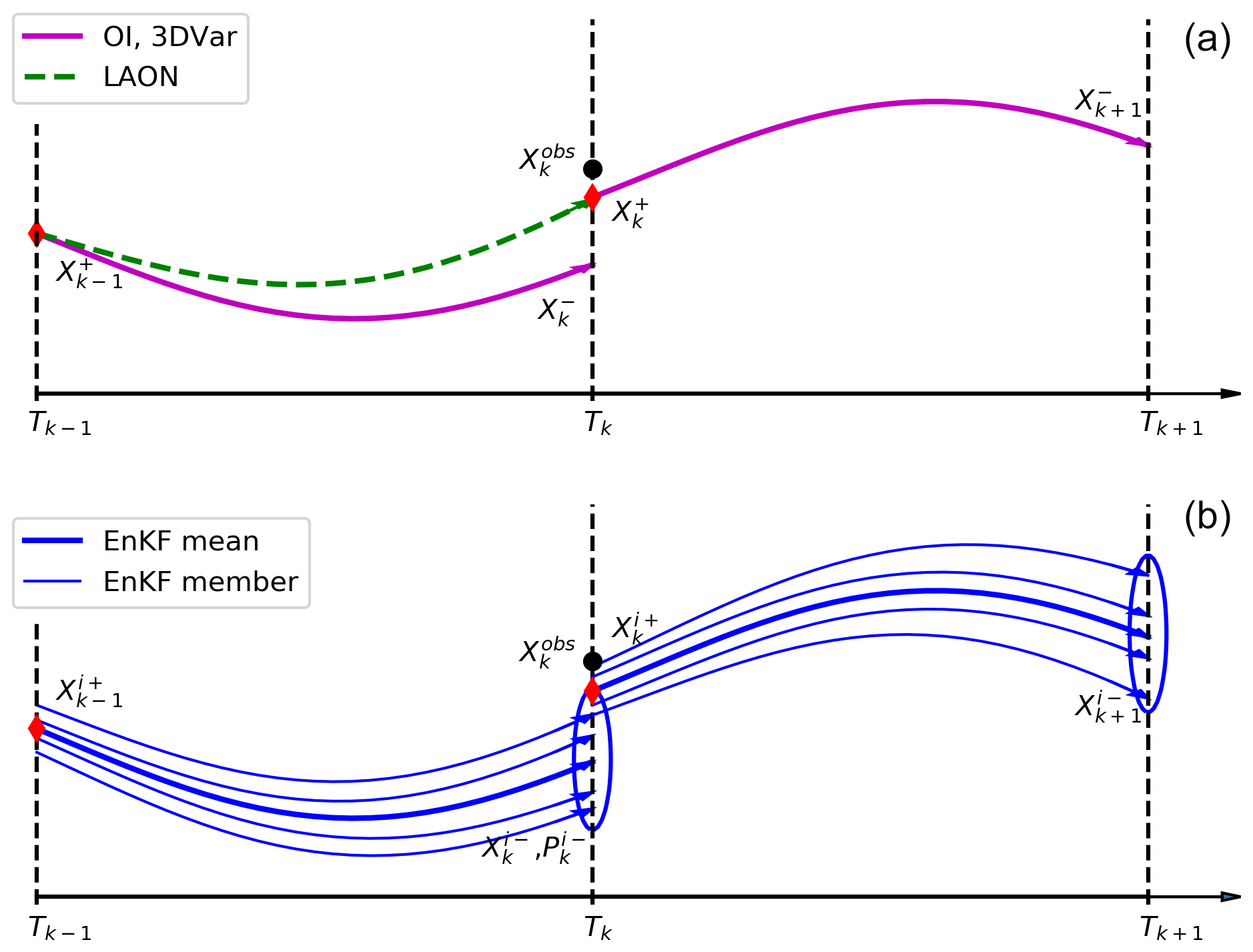
Figure 2A schematic illustrating the assimilation procedures using OI, 3D-Var, LAON (a), and EnKF (b). (black dot) denotes the kth observation at time Tk; and (red diamond) respectively denote the model results before and after assimilation at Tk using OI or 3D-Var for assimilation. The superscript i denotes the ensemble member in the EnKF. The observation time step is , with Δt being the model time step. ΔT and Δt are 1 d and 2.5 min in the present LAON assimilation. Here OI, 3D-Var, LAON, and EnKF represent optimal interpolation, three-dimensional variational, local analytical optimal nudging, and ensemble Kalman filter, respectively. In the lower legend, the EnKF mean is an average of all the EnKF members.
Figure 2 shows a schematic illustrating the assimilation procedures using OI, 3D-Var, LAON, and EnKF. In general, OI and 3D-Var are equivalent when the model and observation error covariances are the same (Lorenc, 1986). As shown in Fig. 2, we denote X as the local variable of X to be assimilated. is the kth observation at time Tk, and and are the model results before and after the assimilation at time Tk when using OI or 3D-Var for assimilation. The time period between two successive observations is , where Δt is the model time step. In the present study, the observation time step is ΔT=1 d and the model time step is Δt=2.5 min, hence N=576.
As a reference, the integration and assimilation using OI or 3D-Var between two successive observations can be expressed as
where the integration of F(X,t) denotes the model free run from Tk−1 to Tk, and K is the Kalman gain which in the local situation is (e.g., Wang et al., 2013)
where σmod and σobs are the standard deviations of the model and observations, respectively. Similarly, when using the EnKF, all the ensemble members will first be integrated after N time steps from Tk−1 and then updated at time Tk, with the optimal estimate being the assimilated ensemble mean which is close to the optimal estimate using OI or 3D-Var.
In contrast to OI, 3D-Var, and EnKF, the LAON assimilation is performed in every model time step (see Fig. 2), which can be expressed for the period from Tk−1 to Tk as
where βK=G is the nudging coefficient, and β is designed as a constant to be determined such that the overall LAON assimilation in the period is equivalent to the single assimilation update using OI or 3D-Var at time Tk (see Fig. 2 and Eq. 6). The initial value is from the integration of the free run following Eq. (5). For simplicity, we denote the observation as Xobs, denote as X0 (the initial value when starting the LAON assimilation at Tk−1), and denote as XN (the final result at Tk after the whole integration). The other intermediate results are denoted as Xj, where . Using a simple forward Euler scheme, the differential LAON assimilation equation (Eq. 8) can be discretized as
where W=βKΔt is the nudging weight. From Eq. (9) we get the contribution from the LAON assimilation at time step j in terms of the initial value X0 and the observation Xobs:
where . According to the original design for the LAON assimilation, Eq. (10) should be equivalent to the OI or 3D-Var single assimilation update in Eq. (6) when j=N. Noting here that , we get the corresponding optimal nudging weight
and the corresponding optimal nudging coefficient
in which β is approximate to the reciprocal of the observation time step. This indicates that the observation time step ΔT is exactly the optimal nudging timescale. For the model error standard deviation, following earlier studies (Wang et al., 2013; Fritzner et al., 2018), we take
With the optimal nudging weight W in Eq. (11), LAON is ready for SIC assimilation in one-category sea ice models using Eq. (9) such that
where aice and aobs are the total model SIC and observed SIC. For multi-category sea ice models, earlier studies designed their assimilations to modify the thinnest sea ice category (e.g., Lindsay and Zhang, 2006; Blockley et al., 2014). In the present multi-category CICE model, we apply a different formulation. When aice>0, Eq. (14) can be rewritten as
Thus, a proportional formulation can be applied to update the ice and snow conditions for all the ice categories such that
where vn and vsn are ice and snow volumes for the nth ice category, and the rate of incremental innovation (see Eq. 15) is modified as
where the function “max” is used to avoid huge values when . In this proportional formulation (Eqs. 16–18), all the variables (an,vn, and vsn) are updated according to the same incremental innovation γ (Eq. 19). Except for situations when the function “max” is activated, this formulation keeps the actual SIT hn and snow depth hsn unchanged during the LAON assimilation. Similarly, the proportions of an, vn, and vsn also remain unchanged when scaled with the total SIC, sea ice volume (SIV) and snow volume. This conservative property facilitates the maintenance of valid sea ice variables during the LAON assimilation.
For the situation when aice=0 and aobs>0, we assume that new model ice will form with the actual SIT hbar is either equal to 0.5 m (Wang et al., 2013) or determined by an empirical formula (Fritzner et al., 2018):
It is noted that in Eq. (20) we have extended the valid range of aobs to (0, 1]. In addition, we set the snow volume as 0.1 of the ice volume, sea ice salinity as 5 PSU, and sea ice temperature at the freezing temperature with the corresponding entropy. Equation (20) is used in the present study.
We choose the following parameters to evaluate the effect of the LAON assimilation of SIC: SIC, sea ice extent (SIE), sea ice area (SIA), SIT, SIV, SST, and SSS. These parameters are generally considered closely related to the SIC. In particular, SIE and SIA are direct products of SIC. As the main focus is on the assimilation of SIC, we use three SIC observations and three CMEMS SIC analyses to thoroughly evaluate the LAON SIC assimilation. The SIT, SST, and SSS data are mainly used to assess the effect of SIC assimilation on the model simulations. All the data were interpolated to the model grid using the nearest-neighbor method.
3.1 SIC observations
In the present study, we use three sources of SIC observation data, namely the AMSR2 SIC, the Special Sensor Microwave Imager/Sounder (SSMIS) SIC, and the NIS ice chart.
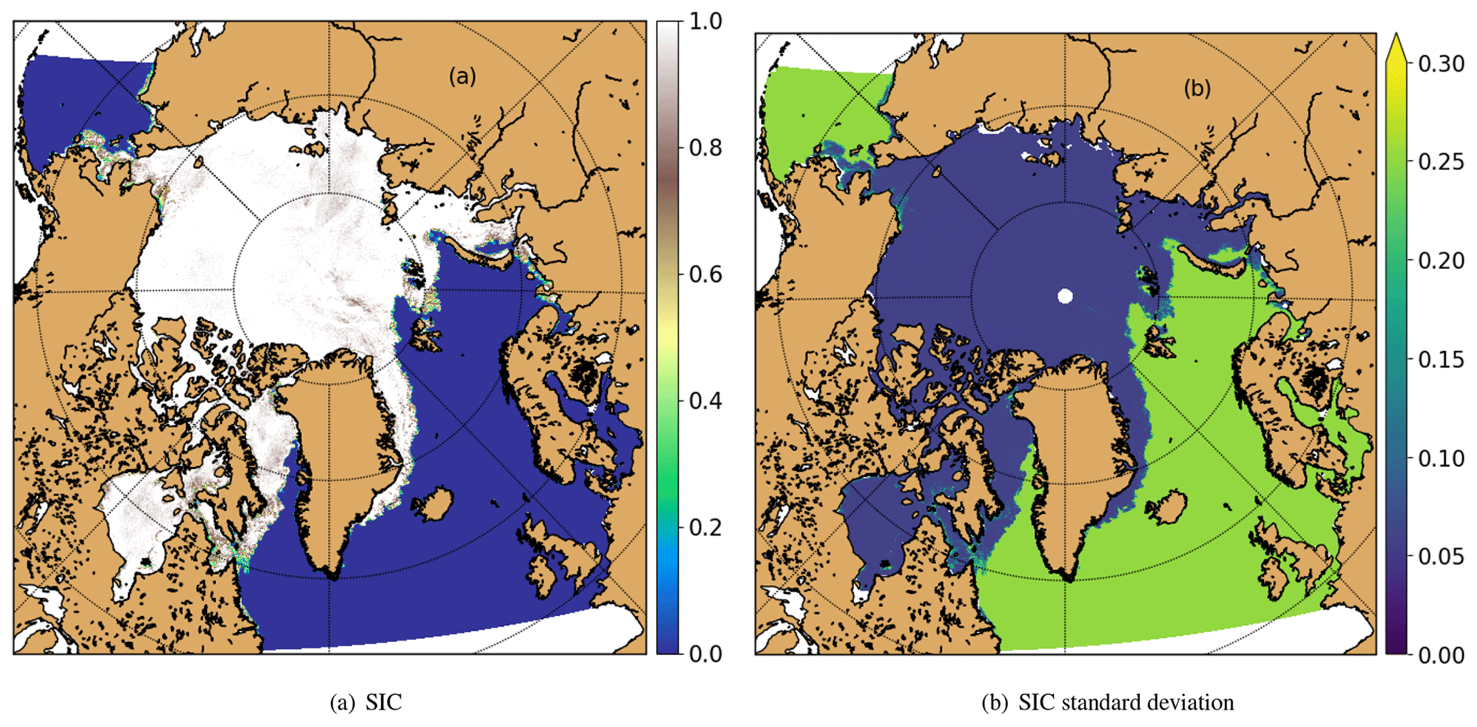
Figure 3AMSR2 SIC and its uncertainty on 1 January 2021. The SIC data are obtained from the University of Bremen.
3.1.1 AMSR2 SIC
The AMSR2 SIC data are from the University of Bremen (https://seaice.uni-bremen.de/data/amsr2/asi_daygrid_swath/n3125/, version 5.4, last access: 17 June 2022) and represent the latest version with a spatial resolution of 3.125 km (Melsheimer, 2019). The AMSR2 on board the GCOM-W1 satellite is a remote sensing instrument for measuring weak microwave emission from the Earth, with a nominal incident angle of 55∘ and swath width of 1450 km. The AMSR2 SIC here uses the same ARTIST sea ice (ASI) algorithm for the AMSR-E 89 GHz channel (Spreen et al., 2008) and is interpolated from the same swath data for the AMSR2 6.25 km SIC product to make the best use of the AMSR2's 89 GHz product (Gunnar Spreen, personal communication, February 2022). The AMSR2 SIC data are the only data being assimilated in this study, and they are also used for evaluation in Sect. 4. Figure 3 shows the SIC and its uncertainty (here standard deviation) on 1 January 2021 from this product. The uncertainty is calculated following the same procedure as in Spreen et al. (2008), where the overall error sums from three sources: radiometric error from the bright temperature, variability of the tie points, and atmospheric opacity. It can be seen that the standard deviation is highest in the open water and lowest in the close drift ice: about 0.25 when SIC = 0 and about 0.057 when SIC = 1 as in Spreen et al. (2008). It is noted that the uncertainties calculated here are fully based on the AMSR2 radiometric properties, the tie-point variability, and the atmospheric opacity. For the open water and MIZ close to the sea ice edge, the high uncertainty is generally realistic and implies that the observed ice edge may be not very accurate. However, for the ice-free areas far away from the sea ice edge (Fig. 3b), the uncertainty should be much lower due mainly to the much higher SST. Such an impact is not considered in the present study. Nevertheless, the high uncertainty in these ice-free areas generally has little effect on the assimilation of the sea ice cover, as the warm ocean surface would enhance the maintenance of the ice-free situation.
3.1.2 SSMIS SIC
The SSMIS SIC is from the EUMETSAT Ocean and Sea Ice Satellite Application Facility (OSISAF; ftp://osisaf.met.no/archive/ice/conc, last access: 18 November 2022). It is an operational product with the product ID OSI-401-b (Tonboe et al., 2017). The SSMIS is a polar-orbiting conically scanning radiometer with an incidence angle around 50∘ and a swath width of about 1700 km. It has window channels near 19, 37, 91, and 150 GHz and sounding channels near 22, 50, 60, and 183 GHz. The SSMIS SIC algorithm uses brightness temperature swath data as input, using the 19V, 37V, and 37H channel data. The brightness temperatures are corrected explicitly for air temperature, wind roughening over open water, and water vapor in the atmosphere prior to the SIC calculation. The algorithm uses dynamical tie points based on the actual mean signatures over the last 30 d. A hybrid algorithm is used which combines the bootstrap (Comiso, 1986) and Bristol (Smith, 1996) frequency-mode algorithms. The results are analyzed on the 10 km OSISAF grid. The SSMIS SIC is the main SIC product assimilated in NEMO (Lellouche et al., 2016) and TOPAZ4 (Hackett et al., 2022). It is also assimilated in neXtSIM together with the AMSR2 SIC (Williams et al., 2021).
3.1.3 NIS ice chart
Due to the large uncertainties in the passive microwave radiometers for low-SIC conditions (e.g., Spreen et al., 2008; Ozsoy-Cicek et al., 2009), we choose the NIS ice chart as an independent SIC product to evaluate the model simulations for sea ice edge and MIZ (Sect. 5). It is from the CMEMS near-real-time product (https://doi.org/10.48670/moi-00128, last access: June 2022, Copernicus Marine Service, 2022d). The ice chart is produced based on manual interpretation of satellite data (Dinessen and Hackett, 2018), which represents a typical subjective analysis product. Unlike the AMSR2/SSMIS SIC, which only uses passive microwave measurements, ice charting employs a variety of satellite observations to obtain a more realistic sea ice edge and MIZ. The main satellite data used are the weather-independent synthetic aperture radar (SAR) data from RadarSat-2 and Sentinel-1. The analyst also uses visual and infrared data from METOP, NOAA, and MODIS in cloud-free conditions. These satellite data cover the charting area several times a day and are resampled to 1 km grid spacing.
It is noted that the NIS ice chart is only provided during working days and only covers the European side of the Arctic. Nevertheless, the ice chart provides important details for the sea ice edge and MIZ. The NIS ice chart includes six ice types following the WMO Sea Ice Nomenclature (WMO, 2014): fast ice (SIC = ), very closed drift ice (9–), closed drift ice (7–), open drift ice (4–), very open drift ice (1–), and open water (0–). For practical use, a mean value is applied to denote the different ice classes in the ice chart (Dinessen and Hackett, 2018).
3.2 SIC analyses
The three SIC analyses are all from the CMEMS operational products, which are the optimal estimates after data assimilation of the operational models NEMO, TOPAZ4, and neXtSIM. These analyses represent the state-of-the-art operational sea ice forecast products in Europe. New developments are being performed with a focus on improving model physics and spatial resolution, as well as extending biogeochemical predictions.
3.2.1 NEMO SIC
The NEMO SIC analysis is from the CMEMS operational product (https://doi.org/10.48670/moi-00016, last access: May 2022, Copernicus Marine Service, 2022a). It is provided by Mercator Ocean of France through the Operational Mercator Global Ocean Analysis and Forecast System (Lellouche et al., 2016; Galloudec et al., 2022). The system uses version 3.6 of the NEMO model (Madec and the NEMO Team, 2017), with the sea ice component being the multi-category sea ice model LIM3 (Rousset et al., 2015). The system uses a tripolar horizontal grid (Madec and Imbard, 1996) and a 50-level vertical grid with a decreasing resolution from 1 m at the surface to 450 m at the bottom. Its data assimilation system, SAM2 (Système d'Assimilation Mercator), uses a reduced-order Kalman filter derived from the singular evolutive extended Kalman (SEEK) filter (Brasseur and Verron, 2006). The assimilated observations include SIC, SIT, SST, in situ T and S profiles, and sea level. The operational product includes daily and monthly mean files of temperature, salinity, currents, sea level, mixed layer depth, and ice parameters over the global ocean. It also includes hourly mean surface fields of sea level height, temperature, and currents. The global ocean output files are displayed on a grid of ∘ horizontal resolution with regular longitude–latitude equirectangular projection.
3.2.2 TOPAZ4 SIC
The TOPAZ4 SIC analysis is from the CMEMS operational product (https://doi.org/10.48670/moi-00001, last access: May 2022, Copernicus Marine Service, 2022b), which is the nominal product of the CMEMS Arctic Monitoring and Forecasting Center (MFC) for ocean physics (Hackett et al., 2022). It is produced by the Arctic MFC through the operational TOPAZ4 Arctic Ocean and sea ice prediction system (Sakov et al., 2012) using version 2.2.37 of the HYCOM ocean model (Bleck, 2002) coupled to a one-category sea ice model with the EVP rheology (Hunke and Dukowicz, 1997). Its sea ice thermodynamics are described in Drange and Simonsen (1996), with a correction of heat flux for sub-grid-scale ice thickness heterogeneity following Fichefet and Morales Maqueda (1997). The model domain covers the North Atlantic and Arctic basins with a grid spacing of approximately 12–16 km. The model uses 28 hybrid vertical layers, with isopycnal vertical coordinates in the stratified open ocean and z coordinates in the unstratified mixed layer. A 100-member deterministic EnKF is used in TOPAZ4 for assimilation of SIC, SIT, sea ice drift, SST, SSS, sea level anomaly, and in situ T and S profiles (Hackett et al., 2022). The analysis is then interpolated and disseminated to a 12.5 km × 12.5 km grid using polar stereographic projection.
3.2.3 neXtSIM SIC
The neXtSIM SIC is from the CMEMS operational product (https://doi.org/10.48670/moi-00004, last access: May 2022, Copernicus Marine Service, 2022c). It is an hourly product produced by the Arctic MFC through the neXtSIM sea ice prediction system (Hackett et al., 2022). The neXtSIM is a stand-alone sea ice model using the Brittle–Bingham–Maxwell sea ice rheology (Rampal et al., 2019). The model domain covers the central Arctic, excluding the Canadian Archipelago and the Pacific side of the Bering Strait (Williams et al., 2021). The model uses a Lagrangian triangular mesh with the mesh element size approximately 7.5 km from point to the opposite side variable (the side length is approximately 10 km). A remeshing procedure is used to avoid anomalously deformed meshes. The model is forced with surface atmosphere forcing from the ECMWF and ocean forcing from TOPAZ4. The model uses the direct insertion method for assimilation, with the observed SIC from a weighted SSMIS SIC and AMSR2 SIC as well as a fixed model SIC uncertainty of 30 % (Williams et al., 2021). The assimilation is run daily before the forecast is launched. The output variables are hourly SIC, SIT, sea ice drift velocity, and snow depth. The adaptive Lagrangian mesh is interpolated for convenience to a 3 km resolution regular grid using polar stereographic projection.
3.3 Weekly mean CS2SMOS SIT
The weekly mean CS2SMOS SIT is from the ESA (ftp://smos-diss.eo.esa.int/SMOS/L4_SIT/L4/north/, last access: 7 October 2022). It is a weighted mean of the weekly mean SMOS thin SIT (Tian-Kunze et al., 2014) and the weekly mean CryoSat-2 SIT (Laxon et al., 2013), with the spatial “no observation” area interpolated from the surrounding observations using the OI method (Ricker et al., 2017). This weekly averaged product is generated every day at the Alfred Wegener Institute (AWI). The data are available from November 2010 but are only available in the winter seasons (from mid-October to mid-April). The data are projected onto the 25 km EASE2 grid based on a polar aspect spherical Lambert azimuthal equal-area projection (Ricker et al., 2017). This CS2SMOS SIT is used in Sect. 4 for evaluating the effect of SIC assimilation on the SIT simulation.
3.4 OSTIA skin SST
The Operational Sea Surface Temperature and Ice Analysis (OSTIA) diurnal skin SST product is from CMEMS (Wang et al., 2023b). It is an hourly mean skin SST at 0.25∘ × 0.25∘ horizontal resolution, analyzed by the UK Met Office, using in situ and satellite data from infrared radiometers (While and Martin, 2013). The skin SST is the temperature measured by satellite infrared radiometers and can experience a large diurnal cycle. The skin SST L4 product is created by combining (1) the OSTIA foundation SST analysis which uses in situ and satellite observations, (2) the OSTIA diurnal warm layer analysis which uses satellite observations, and (3) a cool skin model. This product is used in Sect. 4 for assessing the effect of SIC assimilation on the SST simulation.
3.5 ISAS SSS
The In Situ Analysis System (ISAS) SSS is also from CMEMS (https://doi.org/10.48670/moi-00037, last access: 15 November 2022, Copernicus Marine Service, 2022e). It is a quality-controlled gridded salinity field based on the objective analysis (OA) of the near-real-time in situ salinity measurements from the Coriolis Database (Szekely and Dobler, 2022). The measurements use a variety of instruments, mainly Argos, moorings, drifting buoys, and sea mammals. The OA is performed monthly using the ISAS tool (Gaillard et al., 2016). The contribution of each quality-controlled salinity observation is first assessed relative to a first guess (climatology). The ISAS SSS is then reconstructed by summing the objectively analyzed anomalies and the first-guess field. It it noted that the analyzed results could be very close to the climatology in poorly sampled areas (Szekely and Dobler, 2022). Nevertheless, it remains one of the best sources of SSS data in the Arctic, particularly under the sea ice. This product is used in Sect. 4 for evaluating the effect of SIC assimilation on the SSS simulation.
The coupled HYCOM–CICE model is initialized and spun up from 2010 using the World Ocean Atlas (WOA) 2018 climatology. A hindcast experiment with and without the LAON data assimilation is performed to evaluate the effect of the LAON assimilation on the model simulations from 1 January 2021 to 30 April 2022. In the following, the experiments with and without data assimilation are denoted as LAON and Free_run, respectively. We use the root mean square error (RMSE) for evaluation. Denoting O(Ok) as the observed variable vector (e.g., SIC, SST, SSS) and M(Mk) as the corresponding model variable vector, we have
where m is the total model grid number (here the observations have been interpolated to the model grid). In addition, we use bias as a supplementary metric, which is a simple mean difference between the model and observations.
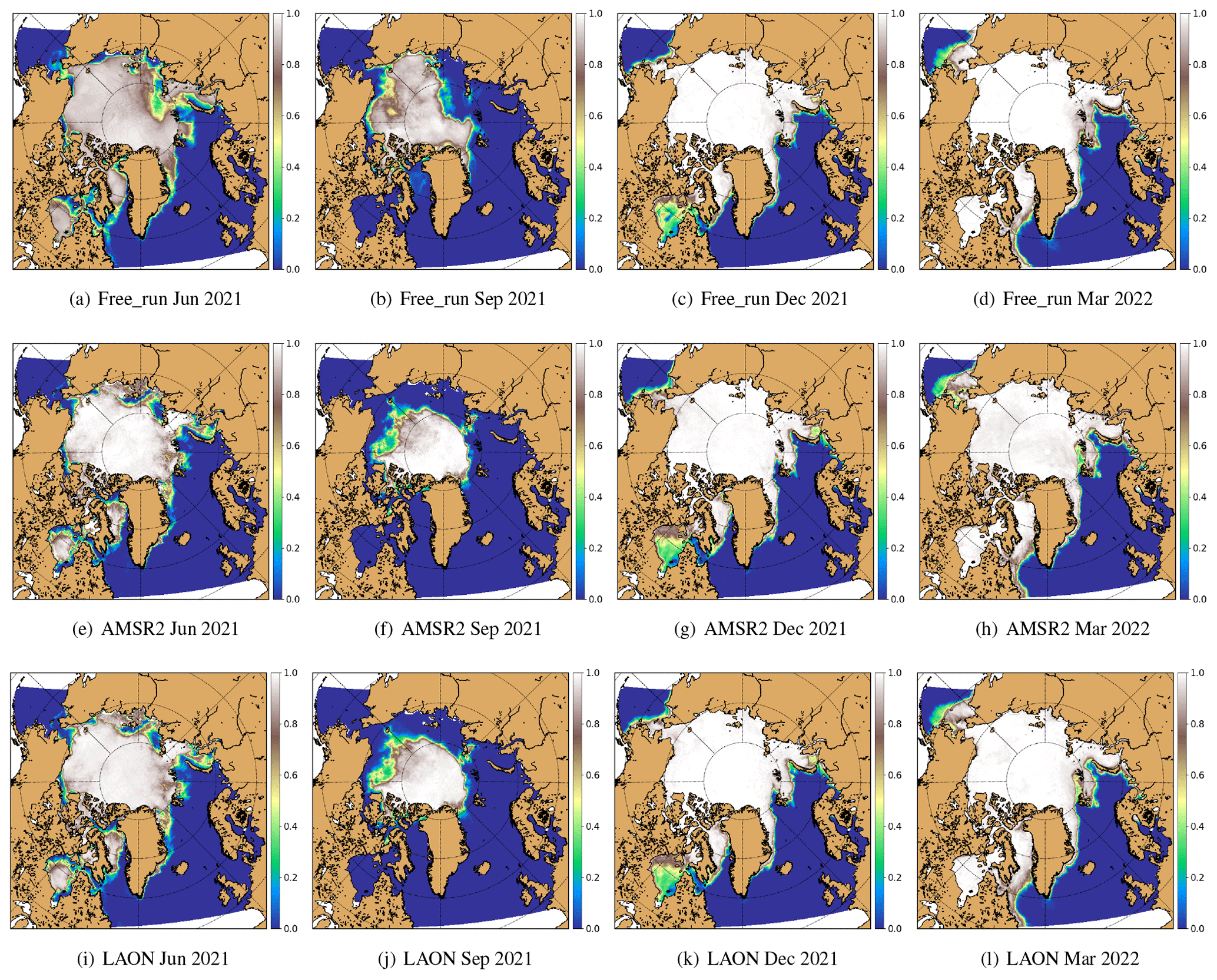
Figure 4Monthly mean SIC from Free_run simulations (a–d), AMSR2 observations (e–h), and LAON simulations (i–l).
4.1 SIC, SIE, and SIA
Figure 4 compares the monthly mean SIC between the Free_run (upper), AMSR2 observations (middle), and the LAON simulation (lower), with the columns from left to right showing the dates June 2021, September 2021, December 2021, and March 2022, respectively. To remove the effect of data assimilation during the early stage, June 2021 is chosen as the starting month for analysis. On the whole, the Free_run simulates the SIC quite well during the winter months (panels c, d vs. g, h in Fig. 4), except for some areas near the sea ice edge. However, there are considerable biases in the simulated SIC during the summer months (panels a, b vs. e, f in Fig. 4). In particular, the simulated September sea ice cover deviates considerably from the observation (panel b vs. f in Fig. 4). By contrast, the LAON assimilation significantly improves the simulation (panels i–l vs. e–h in Fig. 4). The spatial pattern of sea ice cover is particularly well reproduced, for example, in the low-SIC areas in the Beaufort Sea in September 2021 (panel j vs. f in Fig. 4), in the Hudson Bay in December 2021 (panel k vs. g in Fig. 4), and in the northern Barents Shelf (north of Svalbard) in March 2022 (panel l vs. h in Fig. 4).
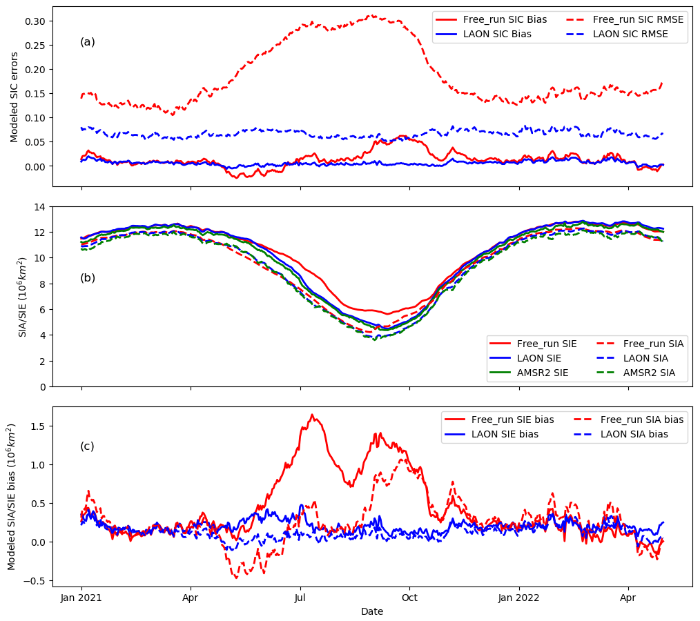
Figure 5Statistics of the simulated SIC, SIE, and SIA: (a) modeled daily SIC mean bias and RMSE, (b) modeled and observed SIE and SIA, and (c) modeled SIE and SIA mean bias.
The daily mean bias and RMSE of the simulated SIC are shown in Fig. 5a. As partly demonstrated in Fig. 4, the Free_run SIC has large RMSE (about 0.3) and relatively low bias during the summer season, indicating large spatial mismatch during the summer season. The low daily bias is mainly due to the offset between the overestimate and underestimate of the SIC in different areas in the Arctic (see also Fig. 4b vs. f). By contrast, the LAON SIC has a much lower daily mean bias and RMSE, with the mean values being 0.006 and 0.066 for the whole period.
SIE and SIA are two derivatives of SIC. In this section, SIE is defined as the total area where SIC ≥0.15, whereas SIA is defined as the total area covered by ice. The simulated (Free_run and LAON) daily SIE and SIA are compared with the AMSR2 observations in Fig. 5b, with their mean bias shown in Fig. 5c. It is seen that all the simulated winter SIE and SIA values agree very well with the AMSR2 observations. However, there are large biases in the Free_run SIE and SIA during the summer season. The mean bias of SIE reaches over 1.0×10⁶ km2 during July to October 2021, which is about 20 % of the observed SIE (see Fig. 5b). The Free_run SIA has a large variation from notably less to significantly larger than the observations as indicated by the daily mean bias and RMSE (Fig. 5c). On the contrary, the mean biases of the LAON SIE and SIA are generally close to 0.2×10⁶ km2, which is about 5 % of the summer SIE and SIA and about 2 % of the winter SIE and SIA.
4.2 SIT and SIV
SIT is not assimilated in the model. This implies that the model SIT will likely deviate from the observation if it was initially biased. To be consistent with the observed weekly mean CS2SMOS SIT, the modeled SIV and SIT have also been averaged weekly. As the CICE model only tracks SIV, the model SIT is calculated here via SIV (SIC ) for each model grid. The observed SIV is calculated via CS2SMOS SIT × AMSR2 SIC for each grid.
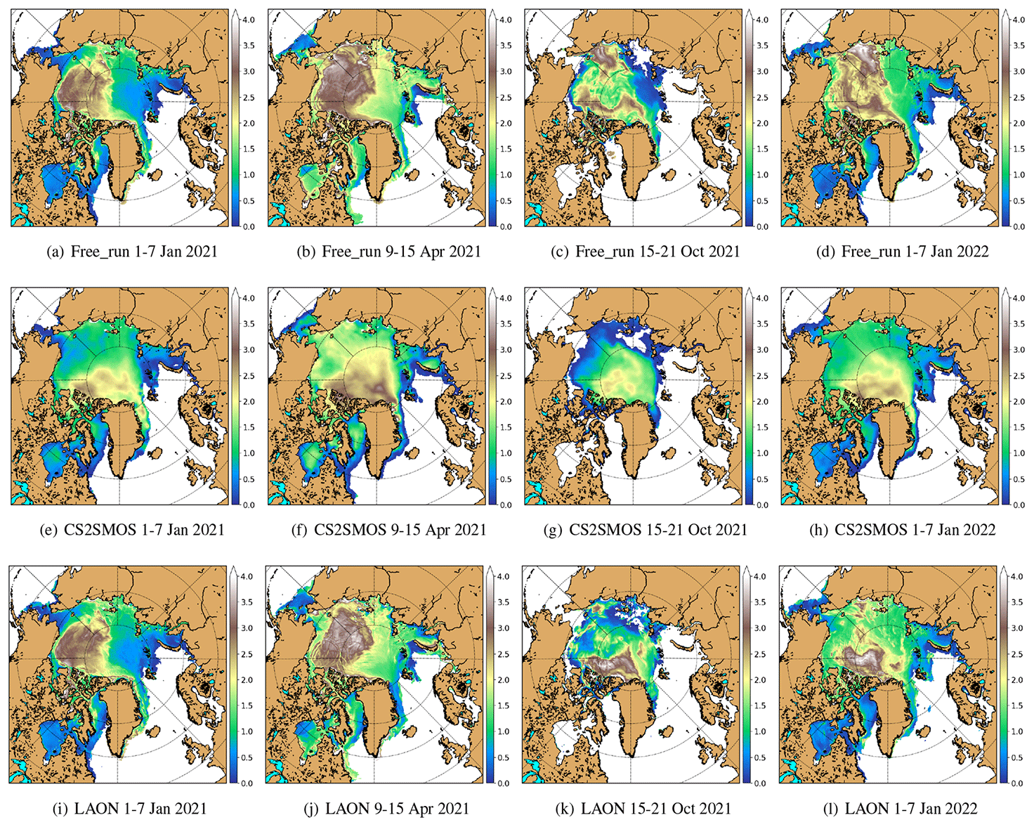
Figure 6Weekly mean SIT (m) from Free_run simulations (a–d), CS2SMOS observations (e–h), and LAON simulations (i–l).
Figure 6 compares the SIT between the Free_run and LAON simulations to the CS2SMOS observations, with the columns from left to right showing the dates 1–7 January 2021, 9–15 April 2021, 15–21 October 2021, and 1–7 January 2022, respectively. It is seen that the model initial SIT fields are considerably biased, with a much larger area of thick multiyear ice (MYI) located in the Beaufort Sea and north of the Canadian Archipelago (Fig. 6a and i), whereas the observed MYI is mainly located north of the Canadian Archipelago and Greenland (Fig. 6e). There is only a mild difference in the Free_run and LAON simulations during the winter period until 9–15 April 2021 (see Figs. 6b and j), both showing the MYI in the Beaufort and East Siberian seas, while the observations show the MYI is mainly located north of the Canadian Archipelago and Greenland (Fig. 6f).
Since the CS2SMOS SIT is only available during the winter period from mid-October to mid-April, we choose the mid-October 2021 to examine the SIT after the summer season (Figs. 6c, g, and k). The overestimated September SIC in the East Siberian Sea in the Free_run simulation (Fig. 4b vs. f) results in significant MYI there in October (Fig. 6c). By contrast, in the LAON simulation most of the MYI in the East Siberian Sea has been replaced by first-year ice (FYI). The MYI is now located mostly to the north of the Canadian Archipelago and Greenland (Fig. 6k), although the thickness is considerably overestimated compared with the CS2SMOS observation (Fig. 6g). It is particularly noteworthy that the LAON simulation produces a much more reasonable spatial SIT pattern in early 2022 (Fig. 6l vs. h), whereas the Free_run simulation returns to a similar pattern as 1 year before (Fig. 6d vs. a).
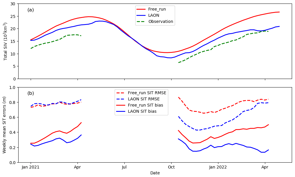
Figure 7Statistics of the simulated SIT and SIV: (a) total SIV as well as (b) modeled SIT mean bias and RMSE.
The initial SIV is about 28.2 % overestimated (Fig. 7a), which corresponds to about 0.23 m thicker than the observation (Fig. 7b). The Free_run SIV is persistently overestimated when compared with the observation during the winter period (CS2SMOS SIT not available during the summer period), with a general increasing bias from November 2021 to April 2022. The LAON SIC assimilation successfully reduces the SIV bias, particularly after the melt season, which is already close to the observations (Fig. 7a). Such improvement can also be clearly seen in the SIT mean bias, where the overall mean bias has dropped to about 0.12 m in April 2022 (Fig. 7b).
The SIT RMSE remains similar between the Free_run and LAON simulations during the early stage from January to April 2021 (Fig. 7b) and differs significantly after the summer period (Fig. 7b). However, the LAON SIT RMSE tends to increase more rapidly than that of the Free_run after November 2021 (Fig. 7b). A detailed check of the sea ice velocity field (not shown) indicates that the exceptionally thick ice north of the Canadian Archipelago and Greenland (see Fig. 6l) considerably affected the sea ice circulation, which is accumulated with time and thus results in a large bias in the SIT fields in the LAON simulations. This problem will be further investigated in a following study with additional assimilation of SIT.
When combining the seasonal evolution of the SIC and SIT fields (Figs. 4 and 6), we can see that the effect of the SIC assimilation on the SIT is the most significant during the summer period. The LAON assimilation effectively corrected the large bias in the spatial distribution of the SIC, particularly in the Arctic shelf seas. Such a correction not only rectifies the summer SIT bias in these areas, but also provides an open-ocean condition close to the observations for the later new ice development during the freezing period. By contrast, the persistent large overestimate in the MYI suggests that the SIC assimilation tends to have limited SIT improvement for the ice that survives through the melt season. Such a mechanism is unanimously applicable to the LAON SIC assimilation when using other SIC products, although the improvement may differ due to the variations in the SIC values and uncertainties.
The effect of the SIC assimilation on the SIT implies that the LAON SIC assimilation would also improve the SIV using any reasonable SIC products, with the largest improvements in the melt season and from new seasonal sea ice formed during the freezing period. While the improvement in the surviving MYI is generally limited, such MYI is expected to be transported out of the Arctic in several years. It is therefore anticipated that, after several years of SIC assimilation, the SIT spatial distribution and the SIV will show an overall improvement. Nevertheless, a direct SIT assimilation would be more effective and prompt.
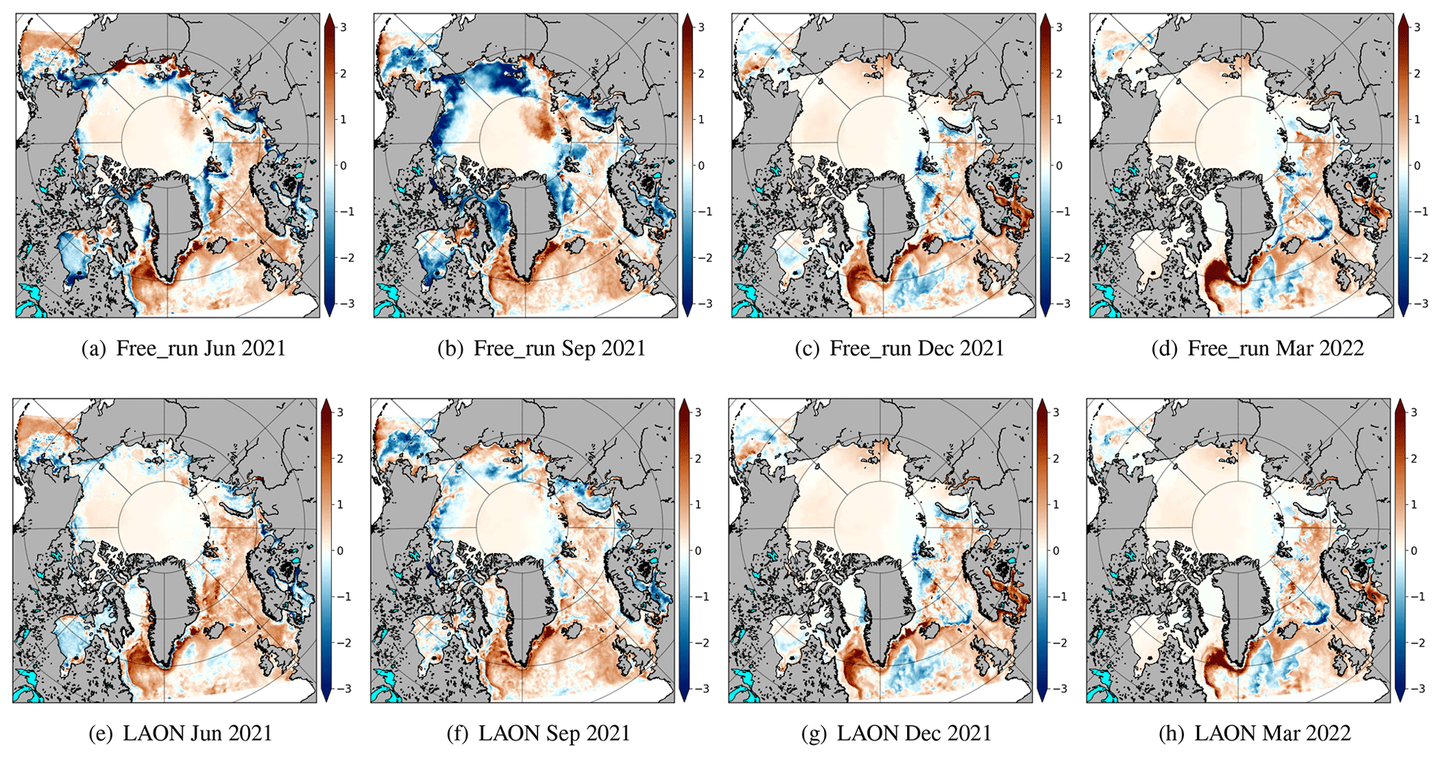
Figure 8Monthly mean SST bias (∘C) from Free_run simulations (a–d) and LAON simulations (e–h). The results are evaluated against the OSTIA monthly mean skin SST from CMEMS.
4.3 SST and SSS
SST is a challenging parameter to define precisely, since the upper ocean has a complex and variable vertical temperature structure related to ocean turbulence and air–sea fluxes of heat, moisture, and momentum. For comparison, we use the top layer model SST, which is the mean temperature of the top 1 m. The hourly OSTIA skin SST is also averaged to obtain the monthly mean SST. Figure 8 compares the monthly mean SST bias between the Free_run and LAON simulations evaluated against the OSTIA monthly mean skin SST. It is noteworthy that the model SST has a positive bias in much of the ice-free area, with the most significant bias around the northern Labrador Sea and southern Davis Strait. Consistent with the SIC (Fig. 4), the SIC assimilation only slightly improved the SST simulations during the winter season (panels c, d vs. g, h in Fig. 8), mainly close to the ice edge. However, during the summer season, the SIC assimilation considerably improved the simulated SST. The Free_run simulation produced a large negative bias in the East Siberian, Chukchi, Beaufort, and Greenland seas and a large positive bias north of the Laptev Sea (Fig. 8b). These biases are considerably mitigated in the LAON simulation (Fig. 8f). It is also noteworthy that in the Baffin and Hudson bays the marked biases in the Free_run are also considerably mitigated in the LAON simulation (panels a, b vs. e, f in Fig. 8).
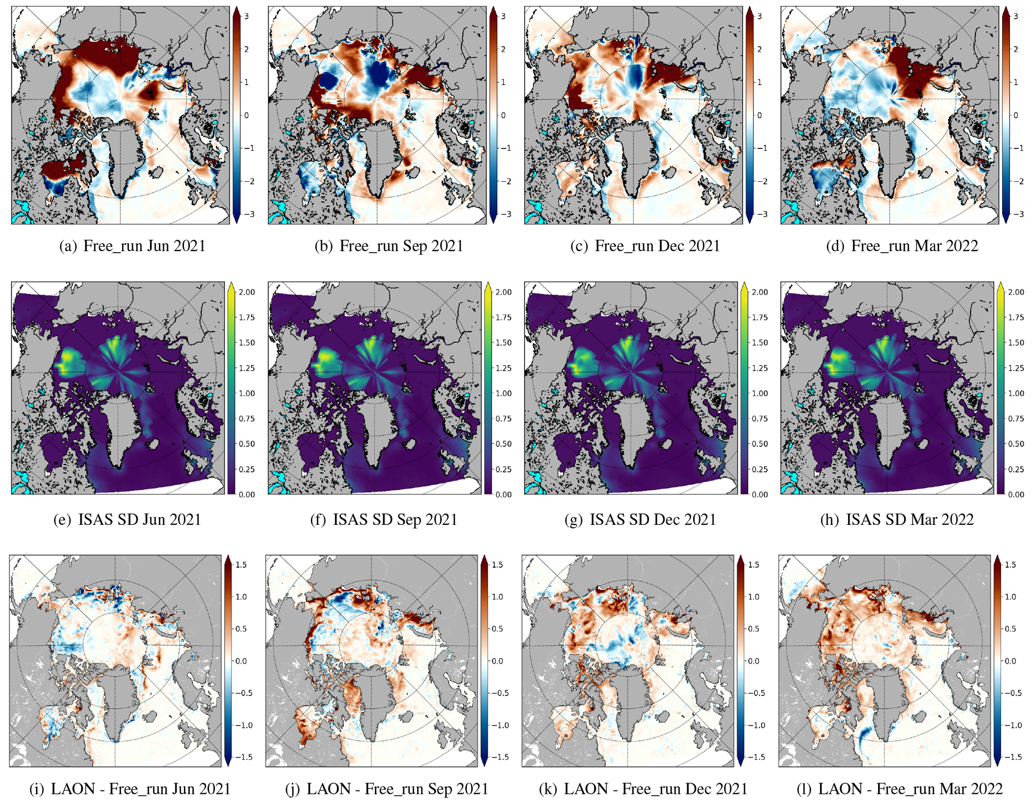
Figure 9Monthly mean SSS bias from Free_run simulations (a–d), ISAS SSS SD (e–h), and modeled SSS difference (i–l). The mean bias is evaluated against the monthly mean ISAS SSS from CMEMS, and SD denotes standard deviation. The modeled SSS difference denotes LAON SSS – Free_run SSS.
Over the large ice-free area in the North Atlantic Ocean, the Free_run simulation reproduces the SSS very well, with the absolute SSS bias generally smaller than 0.5 PSU (Fig. 9a–d). However, there is significant SSS bias in the Arctic. In particular, the SSS is considerably overestimated in much of the Arctic shelf seas, with an occasional large bias even up to 30 PSU. Such large overestimates are likely related to the external forcing of river discharges and inaccurate evaporation–precipitation processes. In addition, there is clear SSS bias in the central Arctic under the sea ice. This tends to suggest that the SSS in the Arctic proper has accumulated a substantial drift during the 10-year spin-up run, as no nudging to the climate was performed under the sea ice. It is noteworthy that these large bias areas in the central Arctic are often collocated with the large uncertainty areas in the observed ISAS SSS (Fig. 9e–h). Further work is needed to clarify the uncertainties and mitigate the deficiencies.
The SSS changes due to the SIC assimilation are much weaker than the absolute SSS bias in the present study. For better illustration, the monthly mean difference between the LAON SSS and Free_run SSS is calculated (Fig. 9i–l). While generally weaker than the absolute bias, the absolute difference over 1 PSU can often be seen in a remarkable part of the Arctic Ocean, particularly in the shelf seas. During the melting season (Fig. 9j), similar to the effect on the SST (Fig. 8), the SIC assimilation notably increases the SSS along the coasts of the Beaufort, Chukchi, New Siberian, Laptev, and Kara seas. The assimilation removes the overestimated sea ice there, thus mitigating the SSS decrease due to the unrealistic sea ice melting. During the freezing period (Fig. 9k, l), unlike the situation for SST which would generally remain close to the freezing point, the SSS tends to continuously increase due to the sea ice freezing and brine rejection. The SSS difference between the LAON and Free_run simulations here is most probably caused by the different sea ice freezing speeds, which are mainly controlled by the corresponding SIT and snow depth. The relatively lower SIT in the LAON simulation (Fig. 6) would foster a more rapid freezing and therefore larger SSS increase during the freezing period. Such a positive increment (Fig. 9l) is seen to counteract the negative bias in the Arctic (Fig. 9d), thus improving the SSS simulation. This is consistent with the findings by Lambert et al. (2019), who identified sea ice melting and brine rejection due to sea ice freezing as playing a dominant role in the Arctic SSS flux in their perfect model experiment using a strong SSS climate restoration. It remains to be seen whether longer-time SIC assimilation can further improve the SSS simulation when no SSS climate restoration is applied.
The meltwater from the Greenland Ice Sheet is not included in the current river discharge. This would induce an overestimate of SSS in the Baffin Bay and Davis Strait, but it would be counteracted by the extra sea ice in the Free_run. The SIC assimilation tends to remove the extra sea ice in September (Fig. 4j), thus recovering the overestimate of SSS in the Baffin Bay and Davis Strait (Fig. 9j). On the whole, an improvement in the external forcing of river discharges including Greenland is highly needed.
SIC is so far one of the most extensively observed sea ice parameters from space. Microwave radiometers such as AMSR2 and SSMIS have the capability to penetrate clouds and continuously monitor the sea ice throughout the year. As a result, they are widely used for sea ice monitoring and data assimilation. However, passive microwave radiometers tend to underestimate low SIC (Spreen et al., 2008; Ozsoy-Cicek et al., 2009). By contrast, the manually analyzed ice chart based on a much larger data set is more reliable for accurately detecting low-SIC areas and sea ice edge (Ozsoy-Cicek et al., 2009; Breivik et al., 2009; Posey et al., 2015). In this section, we evaluate the LAON assimilation by comparing the NorHAPS simulations to the CMEMS operational SIC analyses and the passive microwave radiometer observations, evaluated against the NIS ice chart.
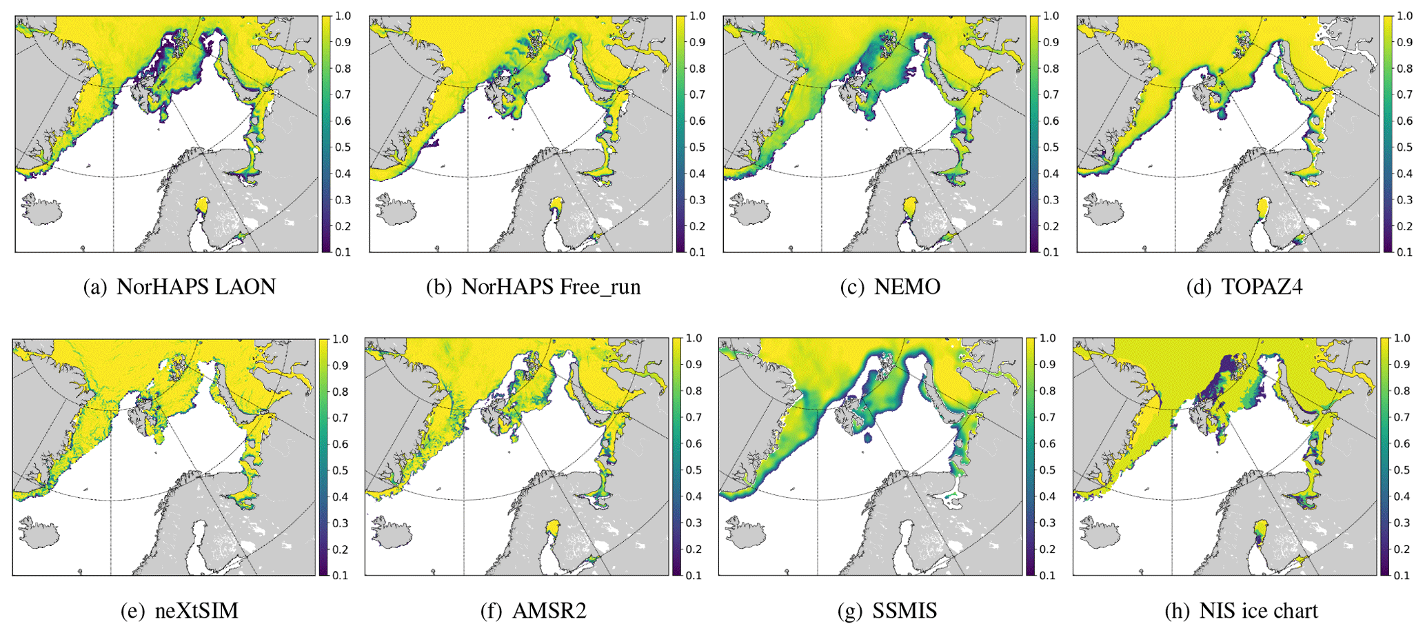
Figure 10Daily SIC on 16 March 2022 from different model analyses and observations. For better illustration of the ice edge, the areas where SIC <0.1 have been removed.
5.1 Daily SIC spatial distribution
Figure 10 compares the daily SIC of the NorHAPS LAON and Free_run with six other daily products for 16 March 2022. Three are from the CMEMS model analyses, namely NEMO, TOPAZ4, and neXtSIM, and the other three are from observations, namely AMSR2, SSMIS, and the NIS ice chart. All the SICs have been interpolated to the NIS ice chart grid. Mid-March is chosen as a typical winter condition. For better demonstration of the ice edge, the areas where SIC <0.1 have been removed. It is noteworthy that NorHAPS LAON assimilated the AMSR2 SIC, NEMO and TOPAZ4 assimilated the SSMIS SIC (Lellouche et al., 2016; Hackett et al., 2022), and neXtSIM assimilated a combined AMSR2 and SSMIS SIC (Williams et al., 2021). The NIS ice chart is not assimilated by any of the models and is therefore an independent observation.
As mentioned above, passive microwave radiometers generally have quite large uncertainties in low-SIC areas. This can also be seen in both AMSR2 (Fig. 10f) and SSMIS (Fig. 10g), where the very open drift ice north of Svalbard seen in the NIS ice chart (Fig. 10h) is missing. Comparing this very open drift ice with the bathymetry (Fig. 1), we see that it collocates very closely with the northern Barents Shelf. This suggests that strong warm Atlantic Water from the west coast of Spitsbergen was turning east and flowing along the northern coast of Svalbard on the northern Barents Shelf, which plays an important role in the melting of sea ice there. The five model analyses generally reproduced most of the sea ice features in the European Arctic (Fig. 10a–e). However, there are large differences among the simulations of the very open drift ice area north of Svalbard and Franz Josef Land. When compared with the NIS ice chart (Fig. 10h), the NEMO SIC analysis (Fig. 10c) is moderately overestimated, showing an area of open drift ice and close drift ice. The NorHAPS Free_run, TOPAZ4, and neXtSIM tend to markedly overestimate the SIC in this very open drift ice area, all showing a large part of very close drift ice (see Fig. 10b, d, and e). By contrast, the NorHAPS LAON (Fig. 10a) produced a simulation close to the observed NIS ice chart, although a small part of the very open drift ice was slightly underestimated as open water. In addition, the open-water and/or ice-free area in the northeastern Barents Sea is well reproduced in the NorHAPS LAON and neXtSIM, whereas a large part was simulated as close or very close drift ice in the NorHAPS Free_run, NEMO, and TOPAZ4. The overall seasonal evolution is assessed through the integrated ice edge error (IIEE) and the integrated MIZ error (IME) below.
5.2 IIEE and IME
The IIEE is determined following Goessling et al. (2016) as
where A denotes the whole model domain, and the subscripts “f” and “t” denote the estimate and the truth (here we use the NIS ice chart as an approximate). The first term on the right side of Eq. (22) denotes the overestimate, and the second term denotes the underestimate. In Goessling et al. (2016), the variable c=1 where SIC >0.15 and c=0 elsewhere. The demarcation value 0.15 is commonly used in the sea ice and climate modeling communities as the sea ice edge. However, this is rather arbitrary as there is no special reason to use 0.15 rather than, e.g., 0.10, as the sea ice edge. In fact, the WMO has used 0.10 as the demarcation between open water and very open drift ice since 1970 (WMO, 2014), which has long been applied in the sea ice charting community, such as the NIS and US National Ice Center ice charts. Therefore, using 0.10 as the demarcation for sea ice edge would be more consistent and helpful for the joint sea ice modeling and observation community. In this section, we use 0.10 as the demarcation for the ice edge.
Following the formulation for the IIEE, we define the IME as
The only difference between Eqs. (23) and (22) is the definition of the variable c. For the IME, c=1 where SIC and c=0 elsewhere.
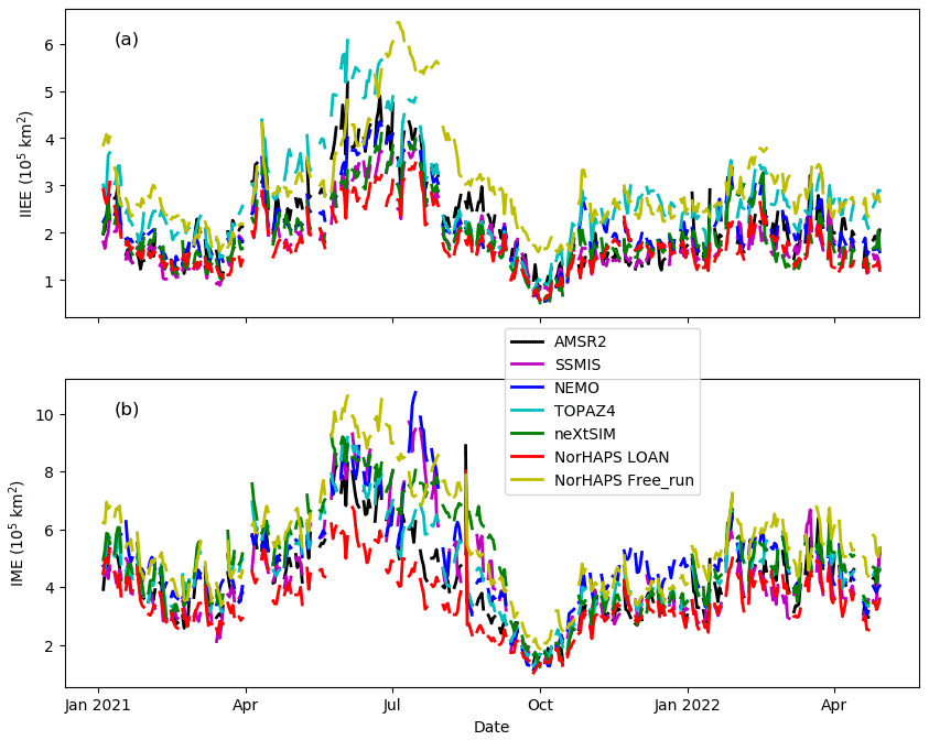
Figure 11Integrated ice edge error (IIEE) and integrated MIZ error (IME) of different SIC products evaluated against the Norwegian ice chart from 1 January 2021 to 30 April 2022: (a) IIEE and (b) IME.
Figure 11 compares the IIEE and IME of NorHAPS LAON and Free_run with two satellite observations (AMSR2 and SSMIS) and three model analyses (NEMO, TOPAZ4 and neXtSIM). All the data are evaluated against the NIS ice chart (total valid data 335). The discontinuities in the IIEE and IME are due to the fact that the NIS ice chart is only available on working days. The Baltic Sea is removed in all the calculations, as neXtSIM does not cover this area. For other areas, if a certain product has no data while the NIS ice chart has a SIC >0.8, then no IIEE and IME are accounted for. This treatment is to remove the coastal effect on other products. On the whole, the IME is about twice the IIEE, indicating that modeling MIZ is considerably more difficult than modeling sea ice edge. It is surprising to see that late September to early October is the time of the lowest IIEE and IME, whereas late June to early July is the time of the largest IIEE and IME; this is ubiquitous in all the observations and model analyses.
As shown in Fig. 5, the Free_run generally has a large bias during the summer period. However, the bias is mainly located in the central Arctic and Pacific marginal seas (Fig. 4), particularly in the Beaufort, Chukchi, and New Siberian seas. For the European Arctic as shown by the NIS ice chart (Fig. 10), the bias is generally moderate (see Fig. 4). This can also be seen in the IIEE and IME (Fig. 11). Except for the summer IIEE which is apparently higher than the other products (Fig. 11a), the Free_run IIEE and IME are generally comparable to the largest IIEE and IME of the other products, although significantly higher than those of LAON.
Table 1Statistics of IIEE and IME for the different SIC products evaluated against the NIS ice chart. The units of the mean and SD of the IIEE and IME are 105 km2, in which SD denotes standard deviation. The p value denotes the probability assuming that the concerned product does not have a statistically different IIEE or IME from NorHAPS LAON.
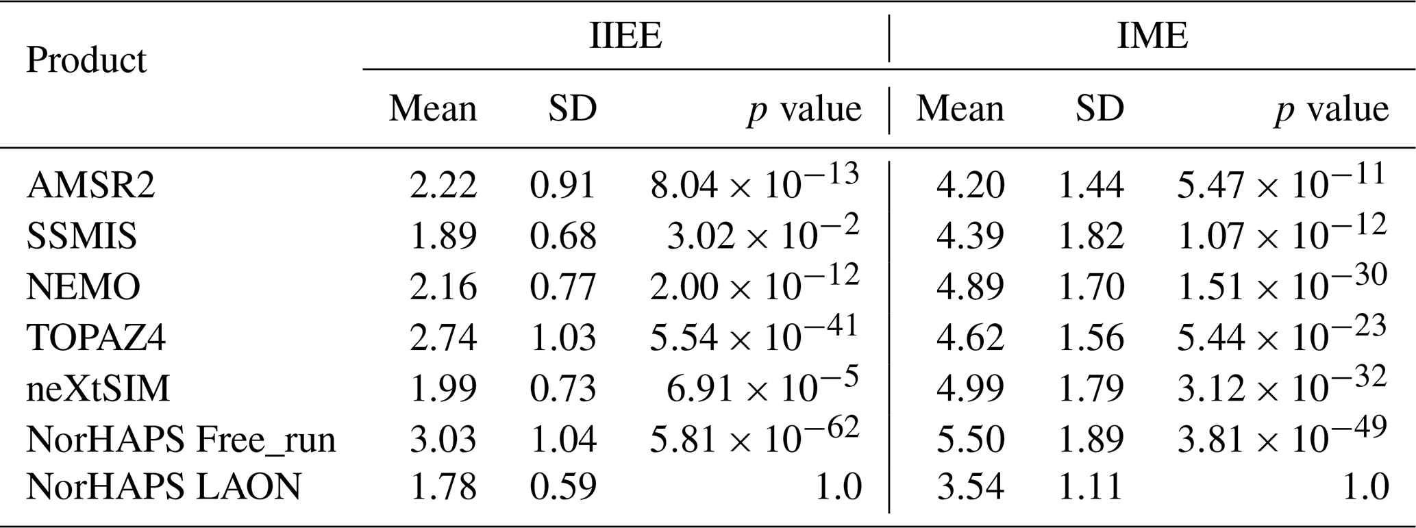
Table 1 summarizes the statistics of the IIEE and IME over the whole period. It is seen that the two observation products AMSR2 and SSMIS SIC have different capabilities to describe the sea ice edge and MIZ. SSMIS has higher capability to capture the sea ice edge, whereas AMSR2 has higher capability to describe the MIZ. The CMEMS analyses (NEMO, TOPAZ4, and neXtSIM) generally have larger IIEE and IME than the SSMIS. TOPAZ4 has a markedly larger bias in the simulated ice edge (see also Fig. 11a); however, it has a better simulation of the MIZ than NEMO and neXtSIM (Fig. 11b). On the contrary, neXtSIM has a relatively small bias in the simulated ice edge but has a large bias in the simulated MIZ, indicating an overestimate of the simulated SIC in the MIZ. This is consistent with the spatial distribution in Fig. 10.
The NorHAPS Free_run has the highest mean IIEE and IME, and the NorHAPS LAON has the lowest IIEE and IME among all the products (Table 1). On average, the IIEE and IME of the Free_run are about 70 % and 55 % higher than those of LAON. Using Welch's unequal variances t test (Welch, 1947), we have estimated the p value (Table 1), which indicates that the probability assuming a concerned product (AMSR2, SSMIS, NEMO, TOPAZ4, neXtSIM, or NorHAPS Free_run) does not have a statistically different mean IIEE and IME from the NorHAPS LAON. It is seen that all the p values are far smaller than 0.01, except SSMIS with a p value of about 0.03 for the IIEE. It is not surprising that the p values for the NorHAPS LAON are both 1.0, since they compare with the data themselves. It is particularly noteworthy that the NorHAPS LAON produces a significantly lower IIEE and IME than the observation AMSR2 SIC that is assimilated in NorHAPS, with the p values both lower than for the IIEE and IME (Table 1). On the whole, the improvement is especially pronounced during the summer season (Fig. 11).
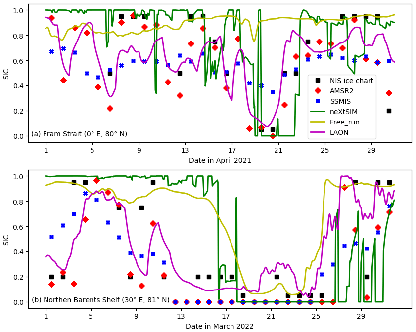
Figure 12Comparison of neXtSIM and NorHAPS hourly SIC close to the sea ice edge: (a) Fram Strait (0∘ E, 80∘ N) in April 2021; (b) northern Barents Shelf (30∘ E, 81∘ N) in March 2022. The exact locations of these two points are shown as a red “x” and “+” in Fig. 1. The NIS ice chart, AMSR2, and SSMIS SIC are daily and added for reference. All the data are interpolated to the corresponding locations using the nearest-neighbor method.
5.3 Hourly evolution
Operational sea ice forecasts rarely provide hourly products, and neXtSIM in CMEMS is an exception. For comparison, we selected two points close to the sea ice edge. One is in the Fram Strait (0∘ E, 80∘ N) in April 2021 and the other in the northern Barents Shelf (30∘ E, 81∘ N) in March 2022, both covering 1 month (Fig. 12). Their exact locations are shown as a red “x” and “+” in Fig. 1. The daily NIS ice chart, AMSR2 SIC, and SSMIS SIC are also added for reference. All the data are interpolated to the two points using the nearest-neighbor method. It is seen that the daily AMSR2 SIC generally has better agreement with the NIS ice chart than the SSMIS SIC. This is partly due to the relatively coarse spatial resolution of the SSMIS SIC, which could have a smoothing effect near the ice edge, averaging high and low SIC.
There are significant differences in the hourly SIC between neXtSIM, Free_run, and LAON. On the whole, neXtSIM tends to overestimate the SIC in the MIZ, as already mentioned (Figs. 10 and 11). For the March 2022 case (Fig. 12b), both neXtSIM and Free_run significantly overestimate the SIC, simulating the very open ice as very close ice. By contrast, the NorHAPS LAON successfully reproduces the evolution of the very open ice as classified by the NIS ice charts. However, for the April 2021 case (Fig. 12a), while the NorHAPS LAON generally captured the overall evolution of the SIC, it tends to underestimate the high SIC, particularly during 7–10 April 2021. By contrast, such high-SIC processes are very well captured by neXtSIM. A further improvement of the NorHAPS model and assimilation system is therefore highly desirable.
The NorHAPS LAON also produces a continuous and smooth change in the local SIC variation. On the contrary, neXtSIM tends to produce abrupt changes in the local SIC (often jumping between 0 and 1 immediately). Such abrupt changes could partly be explained by the physical processes (e.g., damage-induced rapid deformation) in neXtSIM. However, opening or closing of sea ice leads over 3 km wide in 1 h is generally unlikely (considering the neXtSIM spatial resolution of 7 km interpolated to a 3 km grid). More sub-daily observations of the MIZ are needed to clarify such variations.
6.1 Model and observation uncertainties
The overall goal of data assimilation is to find the optimal estimate of the concerned variables, as close as possible to the true values. Such an optimal estimate is generally a weighted average of the model simulations and the observations, with the weights commonly being proportional to the inverse of the error covariance of the model and the observations. Therefore, the uncertainties of the model and the observations provide essential information for data assimilation and need to be seriously treated.
In sea ice observations, uncertainty has gradually become a standard of the operational products, e.g., SMOS SIT (Tian-Kunze et al., 2014), weekly mean CS2SMOS SIT (Ricker et al., 2017), and OSISAF SSMIS SIC (Tonboe et al., 2017; Lavergne et al., 2019). Such estimated uncertainties provide very useful information on the observed sea ice parameters and are thus highly valuable for data assimilation.
Estimating model uncertainty remains one of the most difficult parts of data assimilation. The EnKF provides a feasible way to estimate this uncertainty. However, due to the non-Gaussian distribution of SIC, applying EnKF for SIC uncertainty estimate is very challenging. It can easily be biased or even collapse into zero uncertainty in the winter central Arctic (e.g., Lisæter et al., 2003; Fritzner et al., 2018). In the current LAON assimilation, we have used a very simple formulation (Eq. 13) to approximate the model uncertainty. The results indicate that this simple equation may have captured the essential part of the model uncertainty.
The local covariance assumption in the current LAON assimilation may lose some useful information during the assimilation. However, the heterogeneous spatial distribution of the Arctic sea ice cover, particularly the existence of the sea ice edge, may favor such a local covariance (simplified as variance). In EnKF assimilation such as in the operational TOPAZ4 system, the covariance is calculated from the previous 1 week, which at the ice edge can cause a noticeable mismatch when applying the new analysis. The high resolution, local covariance, concurrent model and observation uncertainties, and continuous assimilation in the LAON method are likely the main reasons for a better simulation of the ice edge and MIZ.
6.2 Data accuracy vs. independence
With continuous development of the remote sensing technique, it has become increasingly common to have multiple observations for the same sea ice variables or parameters. Such multiple data may have different coverage, resolution, and accuracy. An important issue arising from this situation is how to best use the observations in data assimilation and model evaluation or whether we have some criteria to determine the data utilization during data assimilation and model evaluation.
There has been little dispute about selecting appropriate data for data assimilation or model evaluation alone. In general, it is preferable to select the observation data with larger spatial coverage and higher accuracy. For the spatial resolution, a common practice is to choose the observations having the closest resolution to the model, although data with other resolutions are also utilized. There also seems to be implicit agreement in the research community that the data accuracy for model evaluation should not be lower than that for data assimilation, whereas higher resolution and larger coverage are generally preferable but not indispensable. In addition, data independence is often stressed for model evaluation.
According to the timeliness, model evaluation can be separated into two types: analysis evaluation and prediction evaluation. The prediction evaluation can basically be seen as independent of data assimilation. Consider a general data assimilation and prediction evaluation loop: (1) data assimilation of earlier observations, (2) model prediction, and (3) prediction evaluation with new observations. Because the new observations are independent of the earlier observations, there is no inherent conflict between data assimilation and prediction evaluation in terms of independence.
Unlike the prediction evaluation, large disagreement remains on data usage for data assimilation and analysis evaluation in terms of accuracy and independence. When independent, more accurate data are available (generally through other instruments with limited temporal and spatial coverage), these data can be readily applied for analysis evaluation. However, when such data are not available, we have to consider other observations, including those that have already been assimilated. As a common practice, data assimilation is performed earlier than analysis evaluation, where the more accurate data will generally be first used for data assimilation. In this case, no consensus has been reached on whether to preferably use the same more accurate data or to use other independent but less accurate data for analysis evaluation. In data science, evaluating model performance with the data used for training is generally not acceptable because it can easily generate overoptimistic and overfitted models. This is reasonable as the trained model is heavily based on the data. However, data assimilation has an essential difference from the model training. In particular, data assimilation does not change the model itself (not for model parameter estimation). Using the same data for analysis evaluation does not necessarily lead to overoptimistic models, as using other data would have other even more severe limitations. Since the ultimate goal of data assimilation is to provide the optimal estimate, even the application of a cross-validation method for analysis evaluation is not encouraged, as it would lose some optimality by reserving the data from data assimilation. One extreme case is perhaps quite intuitive: a true value (100 % accuracy) would be best for both data assimilation and model evaluation. With low-accuracy independent data, it remains difficult to provide a convincing evaluation. Therefore, accuracy should have a higher priority than independence for analysis evaluation. This again stresses the importance of the estimation of observation uncertainty, which can be seen as a qualitative description of accuracy.
In the present study, we have used two sources of SIC data for model evaluation: AMSR2 SIC and the NIS ice chart. The AMSR2 SIC is assimilated in the present study and is therefore closely related to the model SIC analysis. It is used for SIC evaluation in Sect. 4. The NIS ice chart is an independent observation for evaluating the model SIC analysis, and it is used in Sect. 5 for evaluating the sea ice edge and MIZ. The main reason for such a distinction is that the NIS ice chart provides a more accurate observation of sea ice edge and MIZ, which are often underestimated in passive microwave radiometer observations (e.g., Spreen et al., 2008; Ozsoy-Cicek et al., 2009; Breivik et al., 2009; Posey et al., 2015). On the contrary, the coarse resolution of the NIS ice chart in the SIC space tends to provide a very rough estimate of SIC, so the AMSR2 SIC would be more accurate for SIC evaluation. This suggests that observations may have different accuracies for different model variables, which is helpful to consider during data assimilation and model evaluations.
In this paper, we have introduced the theory of LAON for data assimilation, which is designed to gradually nudge the model value to the optimal estimate. It is applied here for assimilating the AMSR2 SIC into the multi-category CICE model in the Norwegian High-resolution pan-Arctic ocean and sea ice Prediction System: NorHAPS. A hindcast experiment with and without the LAON assimilation is performed, and the results are thoroughly evaluated against a variety of sea ice and ocean observations as well as three CMEMS SIC analyses. Based on the model evaluation, we have the following conclusions.
-
The LAON assimilation of SIC greatly improves the simulation of SIC and its derivatives SIE and SIA. The LAON SIC has a low mean RMSE of about 0.066 for the whole period, whereas the Free_run SIC has a much higher RMSE of about 0.15 during the winter season and 0.3 during the summer season. The LAON assimilation significantly improves the simulated sea ice edge and MIZ evaluated against the NIS ice chart. It produces a significantly lower IIEE and IME than the two passive microwave radiometer observations AMSR2 and SSMIS, as well as the three CMEMS SIC analyses NEMO, TOPAZ4, and neXtSIM, which use EnKFs and direct insertion for data assimilation. LAON also produces a continuous evolution of the simulated SIC, which provides a realistic description of sub-daily SIC evolution with daily observations.
-
The LAON assimilation of SIC improves the simulation of SIT and SIV, with the largest improvements in the melt season and from new seasonal sea ice formed during the freezing period. In the present study, the spatial pattern of the simulated SIT is noticeably improved after a 1-year LAON assimilation. The LAON assimilation also reduces the overestimate of SIV, with the bias in the second year being less than 3000 km3 compared to over 4000 km3 in the Free_run simulation (Fig. 7). However, the LAON assimilation of SIC generally has limited improvement in the surviving MYI, and it may take several years of assimilation to reach a notable improvement. Therefore, a direct assimilation of the SIT is highly needed.
-
The LAON assimilation of SIC improves the SST simulation. In particular, the LAON assimilation considerably mitigates the large summer SST bias in the East Siberian, Chukchi, and Beaufort seas, as well as in the Hudson and Baffin bays. The LAON assimilation of SIC also improves the SST simulation along the sea ice edge throughout the year, with the most pronounced areas in the Greenland and Barents seas. However, the assimilation generally has little impact on the ice-free area in the North Atlantic Ocean.
-
The current NorHAPS reproduces the SSS very well in the ice-free North Atlantic Ocean. However, it tends to produce a large SSS bias in the Arctic, particularly in the shelf seas, which likely results from inaccurate river discharges, precipitation, and evaporation in the model, as well as possible inaccuracy in the initial condition in the Arctic. The SIC assimilation generally has a weaker effect on the simulated SSS than the model SSS bias. Nevertheless, the LAON SIC assimilation provides a reasonable description of the seasonal SSS response to the optimization of the sea ice cover. During the melting season, the SIC assimilation removes the overestimated sea ice, thus mitigating the SSS decrease due to the unrealistic sea ice melting. During the freezing period, the SSS tends to continuously increase due to the sea ice freezing and brine rejection resulting from the relatively lower SIT. A further investigation is needed to mitigate the large model SSS bias.
-
LAON is an efficient data assimilation method. The extra computational cost for the LAON assimilation is negligibly small at about 5 % of the Free_run in the present study. It also has a high capability to simulate the sub-daily evolution when only daily observations are available. These advantages provide a very promising basis for further application in global high-resolution coupled models. In the present study, due to the large bias in the SIT field, our focus has been mainly on the evaluation of the model analysis. Further evaluation of model predictions will be performed in a following study with additional SIT assimilation.
The source code of LAON for assimilating the SIC in the coupled HYCOM–CICE model is available through https://doi.org/10.5281/zenodo.7572286 (Wang and Ali, 2023) tagged as version 0.1.1 of the hycom-cice_coin repository.
The model hindcast experiment data are available at https://doi.org/10.5281/zenodo.7533372 (Wang et al., 2023a). The AMSR2 SIC is available at https://seaice.uni-bremen.de/data/amsr2/ (Melsheimer and Spreen, 2022). The SSMIS SIC is available at https://doi.org/10.15770/EUM_SAF_OSI_NRT_2004 (OSI SAF, 2017). The NIS ice chart is available at https://doi.org/10.48670/moi-00128 (Copernicus Marine Service, 2022d). The NEMO SIC is available at https://doi.org/10.48670/moi-00016 (Copernicus Marine Service, 2022a). The TOPAZ4 SIC is available at https://doi.org/10.48670/moi-00001 (Copernicus Marine Service, 2022b). The neXtSIM SIC is available at https://doi.org/10.48670/moi-00004 (Copernicus Marine Service, 2022c). The weekly mean CS2SMOS SIT is available at ftp://smos-diss.eo.esa.int/SMOS/ (last access: October 2022). The OSTIA skin SST is available at https://doi.org/10.5281/zenodo.10025338 (Wang et al., 2023b). The ISAS SSS is available at https://doi.org/10.48670/moi-00037 (Copernicus Marine Service, 2022e).
KW developed and implemented the LAON method in CICE. KW and AA prepared the data and performed the model simulations. KW, AA, and CW analyzed the results. KW wrote the draft paper, and all authors discussed the results and refined the paper.
The contact author has declared that none of the authors has any competing interests.
Publisher's note: Copernicus Publications remains neutral with regard to jurisdictional claims made in the text, published maps, institutional affiliations, or any other geographical representation in this paper. While Copernicus Publications makes every effort to include appropriate place names, the final responsibility lies with the authors.
The authors are grateful to Gunnar Spreen at the University of Bremen for the discussion about the AMSR2 SIC and Nick Hughes at the Norwegian Ice Service for the discussion about the ice charting. The production of the merged CryoSat-SMOS sea ice thickness data was funded by the ESA project SMOS & CryoSat-2 Sea Ice Data Product Processing and Dissemination Service, and data were obtained from the ESA.
This study was supported by the Norwegian Research Council (grant no. 328886), the Norwegian FRAM Flagship program (grant no. 551323), the Nordic Council of Ministers (grant no. 102642), and the National Key R&D Program of China (grant no. 2022YFE0106300).
This paper was edited by David Schroeder and reviewed by two anonymous referees.
Ali, A., Muller, M., Bertino, L., and Melson, A.: A high resolution three-dimensional model of ocean tides for the pan-arctic region, EGU General Assembly 2021, online, 19–30 April 2021, EGU21-2409, https://doi.org/10.5194/egusphere-egu21-2409, 2021. a
Anthes, R. A.: Data Assimilation and Initialization of Hurricane Prediction Models, J. Atmos. Sci., 31, 702–719, https://doi.org/10.1175/1520-0469(1974)031<0702:DAAIOH>2.0.CO;2, 1974. a, b
Berkman, P. A., Fiske, G., Lorenzini, D., Young, O. R., Pletnikoff, K., Grebmeier, J. M., Fernandez, L. M., Divine, L. M., Causey, D., Kapsar, K. E., and Jørgensen, L. L.: Satellite record of pan-Arctic maritime ship traffic, NOAA technical report OAR ARC, 22-10, https://doi.org/10.25923/mhrv-gr76, 2022. a
Bleck, R.: An oceanic general circulation model framed in hybrid isopycnic-Cartesian coordinates, Ocean Model., 37, 55–88, 2002. a, b
Blockley, E. W., Martin, M. J., McLaren, A. J., Ryan, A. G., Waters, J., Lea, D. J., Mirouze, I., Peterson, K. A., Sellar, A., and Storkey, D.: Recent development of the Met Office operational ocean forecasting system: an overview and assessment of the new Global FOAM forecasts, Geosci. Model Dev., 7, 2613–2638, https://doi.org/10.5194/gmd-7-2613-2014, 2014. a, b
Bouillon, S., Fichefet, T., Legat, V., and Madec, G.: The elastic-viscous-plastic method revisited, Ocean Model., 71, 1–12, 2013. a
Brasseur, P. and Verron, J.: The SEEK filter method for data assimilation in oceanography: a synthesis, Ocean Dynam., 56, 650–661, https://doi.org/10.1007/s10236-006-0080-3, 2006. a
Breivik, L., Carrieres, T., Eastwood, S., Fleming, A., Girard-Ardhuin, F., Karvonen, J., Kwok, R., Meier, W., Mäkynen, M., Pedersen, L., Sandven, S., Similä, M., and Tonboe, R.: Remote Sensing of Sea Ice, ESA Publication WPP-306, Venice, Italy, https://doi.org/10.5270/OceanObs09.cwp.11, 2009. a, b
Buehner, M., Caya, A., Pogson, L., Carrieres, T., and Pestieau, P.: A new environment Canada regional ice analysis system, Atmosphere-Ocean, 51, 18–34, https://doi.org/10.1080/07055900.2012.747171, 2013. a
Caya, A., Buehner, M., and Carrieres, T.: Analysis and forecasting of sea ice conditions with three-dimensional variational data assimilation and a coupled ice–ocean mode, J. Atmos. Ocean. Tech., 27, 353–369, https://doi.org/10.1175/2009jtecho701.1, 2010. a, b, c, d
Cohen, J., Zhang, X., Francis, J., Jung, T., Kwok, R., Overland, J., Ballinger, T. J., Bhatt, U. S., Chen, H. W., Coumou, D., Feldstein, S., Gu, H., Handorf, D., Henderson, G., Ionita, M., Kretschmer, M., Laliberte, F., Lee, S., Linderholm, H. W., Maslowski, W., Peings, Y., Pfeiffer, K., Rigor, I., Semmler, T., Stroeve, J., Taylor, P. C., Vavrus, S., Vihma, T., Wang, S., Wendisch, M., Wu, Y., and Yoon, J.: Divergent consensuses on Arctic amplification influence on midlatitude severe winter weather, Nat. Clim. Change, 10, 20–29, https://doi.org/10.1038/s41558-019-0662-y, 2020. a
Comiso, J. C.: Characteristics of arctic winter sea ice from satellite multispectral microwave observations, J. Geophys. Res., 91, 975–994, https://doi.org/10.1029/JC091iC01p00975, 1986. a
Comiso, J. C.: Large decadal decline of the Arctic multiyear ice cover, J. Cli., 25, 1176–1193, https://doi.org/10.1175/JCLI-D-11-00113.1, 2012. a
Constable, A., Harper, S., Dawson, J., Holsman, K., Mustonen, T., Piepenburg, D., and Rost, B.: Cross-Chapter Paper 6: Polar Region, Cambridge University Press, Cambridge, UK and New York, USA, https://doi.org/10.1017/9781009325844.023, 2022. a, b
Copernicus Marine Service: Global Ocean Physics Analysis and Forecast, Copernicus Marine Service [data set], https://doi.org/10.48670/moi-00016, May 2022a. a, b, c
Copernicus Marine Service: Arctic Ocean Physics Analysis and Forecast, Copernicus Marine Service [data set], https://doi.org/10.48670/moi-00001, last access: May 2022b. a, b
Copernicus Marine Service: Arctic Ocean Sea Ice Analysis and Forecast, Copernicus Marine Service [data set], https://doi.org/10.48670/moi-00004, last access: May 2022c. a, b
Copernicus Marine Service: Arctic Ocean – Sea Ice Concentration Charts – Svalbard and Greenland, Copernicus Marine Service [data set], https://doi.org/10.48670/moi-00128, last access: June 2022d. a, b
Copernicus Marine Service: Global Ocean-Real time in-situ observations objective analysis, Copernicus Marine Service [data set], https://doi.org/10.48670/moi-00037, last access: 15 November 2022e. a, b
Copernicus Marine Service: Arctic Ocean Tidal Analysis and Forecast, Copernicus Marine Service [data set], https://doi.org/10.48670/moi-00005, 2019. a
Dammann, D., Eicken, H., Mahoney, A., Meyer, F., and Betcher, S.: Assessing sea ice trafficability in a changing Arctic, Arctic, 71, 1–113, https://doi.org/10.14430/arctic4701, 2018. a
Dinessen, F. and Hackett, B.: Product user manual for regional high resolution sea ice charts Svalbard region, Copernicus Marine Service, http://marine.copernicus.eu/documents/PUM/CMEMS-OSI-PUM-011-002.pdf (last access: June 2022), 2018. a, b
Drange, H. and Simonsen, K.: Formulation of air-sea fluxes in the ESOP2 version of MICOM, NERSC, Thornøhlensgt., 47, 5006 Bergen, Norway, 1996. a
Eicken, H.: Arctic sea ice needs better forecasts, Nature, 497, 431–433, https://doi.org/10.1038/497431a, 2013. a
Emmerson, C. and Lahn, G.: Arctic opening: Opportunity and risk in the high north, Lloyds Rep., http://library.arcticportal.org/id/eprint/1671 (last access: May 2022), 2012. a
Fairall, C. W., Bradley, E. F., E., H. J., Grachev, A. A., and Edson, J. B.: Bulk parameterization on air–sea fluxes: Updates and verification for the COARE algorithm, J. Climate, 16, 571–591, https://doi.org/10.1175/1520-0442(2003)016<0571:BPOASF>2.0.CO;2, 2003. a
Fichefet, T. and Morales Maqueda, M. A.: Sensitivity of a global sea ice model to the treatment of ice thermodynamics and dynamics, J. Geophys. Res.-Oceans, 102, 12609–12646, https://doi.org/10.1029/97JC00480, 1997. a
Fritzner, S., Graversen, R., Wang, K., and Christensen, K.: Comparison between a multi-variate nudging method and the ensemble Kalman filter for sea-ice data assimilation, J. Glaciol., 64, 387–396, https://doi.org/10.1017/jog.2018.33, 2018. a, b, c, d, e, f, g, h
Gaillard, F., Reynaud, T., Thierry, V., Kolodziejczyk, N., and Von Schuckmann, K.: In-situ based reanalysis of the global ocean temperature and salinity with ISAS: variability of the heat content and steric height, J. Climate, 29, 1305–1323, https://doi.org/10.1175/JCLI-D-15-0028.1, 2016. a
Galloudec, O. L., Chune, S. L., Nouel, L., Fernandez, E., Derval, C., Tressol, M., Dussurget, R., Biardeau, A., and Tonani, M.: Product User Manual for Global Ocean Physical Analysis and Forecasting Product GLOBAL_ANALYSISFORECAST_PHY_001_024, 1.9, Copernicus Marine Service, https://catalogue.marine.copernicus.eu/documents/PUM/CMEMS-GLO-PUM-001-024.pdf (last access: May 2022), 2022. a
Goessling, H. F., Tietsche, S., Day, J. J., Hawkins, E., and Jung, T.: Predictability of the Arctic sea ice edge, Geophys. Res. Lett., 43, 1642–1650, https://doi.org/10.1002/2015GL067232, 2016. a, b
Hackett, B., Bertino, L., Ali, A., Burud, A., Williams, T., Xie, J., Yumruktepe, C., Wakamatsu, T., and Melsom, A.: PRODUCT USER MANUAL For Arctic Ocean Physical and BGC Analysis and Forecasting Products ARCTIC_ANALYSIS_FORECAST_PHY_002_001_a, Issue: 5.15, Copernicus Marine Service, https://catalogue.marine.copernicus.eu/documents/PUM/CMEMS-ARC-PUM-002-ALL.pdf (last access: May 2022), 2022. a, b, c, d, e
Hibler, W. D.: A dynamic thermodynamic sea ice model, J. Phys. Oceanogr., 9, 817–846, https://doi.org/10.1175/1520-0485(1979)009<0815:ADTSIM>2.0.CO;2, 1979. a
Hibler, W. D.: Modeling a variable thickness sea ice cover, Mon. Weather Rev., 108, 1943–1973, https://doi.org/10.1175/1520-0493(1980)108<1943:MAVTSI>2.0.CO;2, 1980. a, b
Hunke, E. and Dukowicz, J. K.: An elastic-viscous-plastic model for sea ice dynamics, J. Phys. Oceanogr., 27, 1849–1867, https://doi.org/10.1175/1520-0485(1997)027<1849:AEVPMF>2.0.CO;2, 1997. a, b, c
Hunke, E., Hebert, D., and Lecomte, O.: Level-ice melt ponds in the Los Alamos sea ice model, CICE, Ocean Mod., 71, 26–42, https://doi.org/10.1016/j.ocemod.2012.11.008, 2013. a
Hunke, E., Lipscomb, W., Turner, A., Jeffery, N., and Elliott, S.: CICE: the Los Alamos Sea Ice Model Documentation and Software User's Manual, Version 5.1, LA-CC-06-012, http://www.ccpo.odu.edu/~klinck/Reprints/PDF/cicedoc2015.pdf (last access: 2020), 2015. a, b, c, d, e
Jung, T., Gordon, N. D., Bauer, P., Bromwich, D. H., Chevallier, M., Day, J. J., Dawson, J., Doblas-Reyes, F., Fairall, C., Goessling, H. F., Holland, M., Inoue, J., Iversen, T., Klebe, S., Lemke, P., Losch, M., Makshtas, A., Mills, B., Nurmi, P., Perovich, D., Reid, P., Renfrew, I. A., Smith, G., Svensson, G., Tolstykh, M., and Yang, Q.: Advancing polar prediction capabilities on daily to seasonal time scales, B. Am. Meteorol. Soc., 97, 1631–1647, https://doi.org/10.1175/BAMS-D-14-00246.1, 2016. a
Kacimi, S. and Kwok, R.: Arctic snow depth, ice thickness, and volume from ICESat-2 and CryoSat-2: 2018–2021, Geophys. Res. Lett., 49, e2021GL097448, https://doi.org/10.1029/2021GL097448, 2022. a
Kwok, R.: Arctic sea ice thickness, volume, and multiyear ice coverage: losses and coupled variability (1958–2018), Environ. Res. Lett., 13, 105005, https://doi.org/10.1088/1748-9326/aae3ec, 2018. a
Lambert, E., Nummelin, A., Pemberton, P., and Ilıcak, M.: Tracing the imprint of river runoff variability on Arctic water mass transformation., J. Geophys. Res.-Oceans, 124, 302–319, https://doi.org/10.1029/2017JC013704, 2019. a
Lavergne, T., Sørensen, A. M., Kern, S., Tonboe, R., Notz, D., Aaboe, S., Bell, L., Dybkjær, G., Eastwood, S., Gabarro, C., Heygster, G., Killie, M. A., Brandt Kreiner, M., Lavelle, J., Saldo, R., Sandven, S., and Pedersen, L. T.: Version 2 of the EUMETSAT OSI SAF and ESA CCI sea-ice concentration climate data records, The Cryosphere, 13, 49–78, https://doi.org/10.5194/tc-13-49-2019, 2019. a
Laxon, S., Giles, K. A., Ridout, A. L., Wingham, D. J., Willatt, R., Cullen, R., Kwok, R., Schweiger, A., Zhang, J., Haas, C., Hendricks, S., Krishfield, R., Kurtz, N., Farrelland, S., and Davidson, M.: CryoSat-2 estimates of Arctic sea ice thickness and volume, Geophys. Res. Lett., 40, 732–737, https://doi.org/10.1002/grl.50193, 2013. a
Lellouche, J.-M., Le Galloudec, O., Regnier, C., Van Gennip, S., Law Chune, S., Levier, B., Greiner, E., Drevillon, M., and Szczypta, C.: Quality Information Document for Global Sea Physical Analysis and Forecasting Product GLOBAL_ANALY-SISFORECAST_PHY_001_024, 1.0, Copernicus Marine Service, https://oceanrep.geomar.de/id/eprint/46419/1/CMEMS-GLO-QUID-001-024.pdf (last access: May 2022), 2016. a, b, c
Lindsay, R. W. and Zhang, J.: Assimilation of ice concentration in an ice–ocean model., J. Atmos. Ocean. Tech., 23, 742–749, https://doi.org/10.1175/jtech1871.1, 2006. a, b, c, d
Lindström, G., Pers, C., J., R., Strömqvist, J., and Arheimer, B.: Development and testing of the HYPE (Hydrological Predictions for the Environment) water quality model for different spatial scales, Hydrol. Res., 41, 295–319, https://doi.org/10.2166/nh.2010.007, 2010. a
Lipscomb, W. and Hunke, E.: Modeling sea ice transport using incremental remapping, Mon. Weather Rev., 132, 1341–1354, https://doi.org/10.1175/1520-0493(2004)132<1341:MSITUI>2.0.CO;2, 2004. a
Lipscomb, W., Hunke, E., Maslowski, W., and Jakacki, J.: Improving ridging schemes for high-resolution sea ice models, J. Geophy. Res.-Ocean, 112, C03S91, https://doi.org/10.1029/2005JC003355, 2007. a
Lisæter, K. A., Rosanova, J., and Evensen, G.: Assimilation of ice concentration in a coupled ice–ocean model using the Ensemble Kalman filter, Ocean Dynam., 53, 368–388, https://doi.org/10.1007/s10236-003-0049-4, 2003. a, b
Lorenc, A. C.: Analysis methods for numerical weather prediction, Quat. J. Roy. Meteor. Soc., 112, 1177–1194, https://doi.org/10.1002/qj.49711247414, 1986. a
Lyard, F. H., Allain, D. J., Cancet, M., Carrère, L., and Picot, N.: FES2014 global ocean tide atlas: design and performance, Ocean Sci., 17, 615–649, https://doi.org/10.5194/os-17-615-2021, 2021. a
Madec, G. and Imbard, M.: A global ocean mesh to overcome the North singularity, Clim. Dynam., 12, 381–388, https://doi.org/10.1007/BF00211684, 1996. a
Madec, G. and the NEMO Team: NEMO ocean engine, Version v3.6, Institut Peirre-Simon Laplace (IPSL), Paris, France, Zenodo, https://doi.org/10.5281/zenodo.1472492, 2017. a
Mathiot, P., König Beatty, C., Fichefet, T., Goosse, H., Massonnet, F., and Vancoppenolle, M.: Better constraints on the sea-ice state using global sea-ice data assimilation, Geosci. Model Dev., 5, 1501–1515, https://doi.org/10.5194/gmd-5-1501-2012, 2012. a, b
Maykut, G. A. and Perovich, D. K.: The role of shortwave radiation in the summer decay of a sea ice cover, J. Geophy. Res., 92, 7032–7044, https://doi.org/10.1029/JC092iC07p07032, 1987. a
Meier, W., Hovelsrud, G., van Oort, B., Key, J., Kovacs, K., Michel, C., Haas, C., Granskog, M., Gerland, S., Perovich, D., Makshtas, A., and Reist, J. D.: Arctic sea ice in transformation: A review of recent observed changes and impacts on biology and human activity, Rev. Geophy., 51, 185–217, https://doi.org/10.1002/2013RG000431, 2014. a, b
Melsheimer, C.: ASI Version 5 Sea Ice Concentration User Guide, Version V0.92, Unversity of Bremen, https://seaice.uni-bremen.de/fileadmin/user_upload/ASIuserguide.pdf (last access: January 2022), 2019. a
Melsheimer, C. and Spreen, G.: AMSR2 ASI sea ice concentration data, Arctic, version 5.4, grid resolution: 3.125 km (July 2012–today), https://seaice.uni-bremen.de/data/amsr2/, last access: June 2022. a
OSI SAF: Global Sea Ice Concentration (SSMIS), OSI-401-d, EUMETSAT Ocean and Sea Ice Satellite Application Facility, https://doi.org/10.15770/EUM_SAF_OSI_NRT_2004, 2017. a
Ozsoy-Cicek, B., Xie, H., Ackley, S. F., and Ye, K.: Antarctic summer sea ice concentration and extent: comparison of ODEN 2006 ship observations, satellite passive microwave and NIC sea ice charts, The Cryosphere, 3, 1–9, https://doi.org/10.5194/tc-3-1-2009, 2009. a, b, c, d
PAME: Arctic shipping Status Report (ASSR) #1: The Increase in Arctic Shipping 2013-2019, Arctic Council, https://pame.is/projects/arctic-marine-shipping/arctic-shipping-status-reports (last access: May 2022), 2020. a
Posey, P. G., Metzger, E. J., Wallcraft, A. J., Hebert, D. A., Allard, R. A., Smedstad, O. M., Phelps, M. W., Fetterer, F., Stewart, J. S., Meier, W. N., and Helfrich, S. R.: Improving Arctic sea ice edge forecasts by assimilating high horizontal resolution sea ice concentration data into the US Navy's ice forecast systems, The Cryosphere, 9, 1735–1745, https://doi.org/10.5194/tc-9-1735-2015, 2015. a, b, c
Rampal, P., Dansereau, V., Olason, E., Bouillon, S., Williams, T., Korosov, A., and Samaké, A.: On the multi-fractal scaling properties of sea ice deformation, The Cryosphere, 13, 2457–2474, https://doi.org/10.5194/tc-13-2457-2019, 2019. a
Ricker, R., Hendricks, S., Kaleschke, L., Tian-Kunze, X., King, J., and Haas, C.: A weekly Arctic sea-ice thickness data record from merged CryoSat-2 and SMOS satellite data, The Cryosphere, 11, 1607–1623, https://doi.org/10.5194/tc-11-1607-2017, 2017. a, b, c
Rothrock, D.: The energetics of the plastic deformation of pack ice by ridging, J. Geophys. Res.-Oceans, 80, 4514–4519, https://doi.org/10.1029/JC080i033p04514, 1975. a, b
Rousset, C., Vancoppenolle, M., Madec, G., Fichefet, T., Flavoni, S., Barthélemy, A., Benshila, R., Chanut, J., Levy, C., Masson, S., and Vivier, F.: The Louvain-La-Neuve sea ice model LIM3.6: global and regional capabilities, Geosci. Model Dev., 8, 2991–3005, https://doi.org/10.5194/gmd-8-2991-2015, 2015. a
Sakov, P., Counillon, F., Bertino, L., Lisæter, K. A., Oke, P. R., and Korablev, A.: TOPAZ4: an ocean-sea ice data assimilation system for the North Atlantic and Arctic, Ocean Sci., 8, 633–656, https://doi.org/10.5194/os-8-633-2012, 2012. a, b
Smith, D. M.: Extraction of winter total sea-ice concentration in the Greenland and Barents Seas from SSM/I data, Int. J. Remote Sens., 17, 2625–2646, https://doi.org/10.1080/01431169608949096, 1996. a
Smith, L. C. and Stepheson, S. R.: New Trans-Arctic shipping routes navigable by midcentury, P. Natl. Acad. Sci. USA, 110, E1191–E1195, https://doi.org/10.1073/pnas.1214212110, 2013. a
Spreen, G., Kaleschke, L., and Heygster, G.: Sea ice remote sensing using AMSR-E 89-GHz channels, J. Geophys. Res.-Oceans, 113, C02S03, https://doi.org/10.1029/2005jc003384, 2008. a, b, c, d, e, f
Stark, J. D., Ridley, J., Martin, M., and Hines, A.: Sea ice concentration and motion assimilation in a sea ice–oceanmodel, J. Geophys. Res.-Oceans, 113, C05S91, https://doi.org/10.1029/2007JC004224, 2008. a
Stauffer, D. R. and Seaman, N. L.: Use of four dimensional data assimilation in a limited area mesoscale model – Part 1: Experiments with synoptic-scale data, Mon. Weather Rev., 118, 1250–1277, https://doi.org/10.1175/1520-0493(1990)118<1250:UOFDDA>2.0.CO;2, 1990. a
Stroeve, J. and Notz, D.: Changing state of Arctic sea ice across all season, Environ. Res. Lett., 13, 103001, https://doi.org/10.1088/1748-9326/aade56, 2018. a
Sumata, H., de Steur, L., Divine, D. V., Granskog, M. A., and Gerland, S.: Regime shift in Arctic Ocean sea ice thickness, Nature, 615, 443–449, https://doi.org/10.1038/s41586-022-05686-x, 2023. a
Szekely, T. and Dobler, D.: Quality information document for In-Situ TAC OA products INSITU_GLO_PHY_TS_OA_NRT_013_002, Copernicus Marine Service, https://catalogue.marine.copernicus.eu/documents/QUID/CMEMS-INS-QUID-013-002.pdf (last access: May 2022), 2022. a, b
Thorndike, A., Rothrock, D., Maykut, G., and Colony, R.: The thickness distribution of sea ice, J. Geophys. Res., 80, 4501–4513, https://doi.org/10.1029/JC080i033p04501, 1975. a, b
Tian-Kunze, X., Kaleschke, L., Maaß, N., Mäkynen, M., Serra, N., Drusch, M., and Krumpen, T.: SMOS-derived thin sea ice thickness: algorithm baseline, product specifications and initial verification, The Cryosphere, 8, 997–1018, https://doi.org/10.5194/tc-8-997-2014, 2014. a, b
Tietsche, S., Notz, D., Jungclaus, J. H., and Marotzke, J.: Assimilation of sea-ice concentration in a global climate model – physical and statistical aspects, Ocean Sci., 9, 19–36, https://doi.org/10.5194/os-9-19-2013, 2013. a, b
Tonboe, R., J., L., Pfeiffer, R., and Howe, E.: Ocean and Sea Ice SAF Product User Manual for OSI SAF Global Sea Ice Concentration Product OSI-401-b, EUMATSAT OSI SAF, https://osisaf-hl.met.no/sites/osisaf-hl.met.no/files/user_manuals/osisaf_cdop3_ss2_pum_ice-conc_v1p6.pdf (last access: November 2022), 2017. a, b
Turner, A. K., Hunke, E. C., and Bitz, C. M.: Two modes of sea-ice gravity drainage: A parameterization for large-scale modeling, J. Geophys. Res.-Oceans, 118, 2279–2294, https://doi.org/10.1002/jgrc.20171, 2013. a
Vidard, P., Le Dimet, F.-X., and Piacentini, A.: Determination of optimal nudging coefficients, Tellus A, 55, 1–15, https://doi.org/10.3402/tellusa.v55i1.14576, 2003. a
Wang, K. and Ali, A.: keguangw/hycom-cice_coin: LAON assimilation of SIC (v0.1), Zenodo [code], https://doi.org/10.5281/zenodo.7572286, 2023. a
Wang, K., Debernard, J., Sperrevik, A. K., Isachsen, P. E., and Lavergne, T.: A combined optimal interpolation and nudging scheme to assimilate OSISAF sea-ice concentration into ROMS, Ann. Glaciol., 64, 8–12, https://doi.org/10.3189/2013aog62a138, 2013. a, b, c, d, e, f, g
Wang, K., Ali, A., and Wang, C.: SIC, SIT, SST and SSS from HYCOM-CICE with LAON assimilation of SIC, Zenodo [data set], https://doi.org/10.5281/zenodo.7533372, 2023a. a
Wang, K., Ali, A., and Wang, C.: SIC, SIT, SST and SSS from HYCOM-CICE with LAON assimilation of SIC (Version V2), Zenodo [data set], https://doi.org/10.5281/zenodo.10025338, 2023b. a, b
Waters, J., Lea, D., Martin, M., Mirouze, I., Weaver, A., and While, J.: Implementing a variational data assimilation system in an operational 1/4 degree global ocean model, Quart. J. Roy. Meteorol. Soc., 141, 333–349, https://doi.org/10.1002/qj.2388, 2015. a
Welch, B. L.: The generalization of Student’s problem when several different population variances are involved, Biometrika., 34, 28–35, https://doi.org/10.1093/biomet/34.1-2.28, 1947. a
While, J. and Martin, M.: Development of a variational data assimilation system for the diurnal cycle of sea surface temperature, J. Geophys. Res.-Oceans, 118, 2845–2862, https://doi.org/10.1002/jgrc.20215, 2013. a
Williams, T., Korosov, A., Rampal, P., and Ólason, E.: Presentation and evaluation of the Arctic sea ice forecasting system neXtSIM-F, The Cryosphere, 15, 3207–3227, https://doi.org/10.5194/tc-15-3207-2021, 2021. a, b, c, d, e
WMO: SEA ICE NOMENCLATURE, No. 259, WMO, https://library.wmo.int/doc_num.php?explnum_id=4651 (last access: May 2022), 2014. a, b
Yang, Q., Losa, S. N., Losch, M., Tian-Kunze, X., Nerger, L., Liu, J., Kaleschke, L., and Zhang, Z.: Assimilating SMOS sea ice thickness into a coupled ice-ocean model using a local SEIK filter, J. Geophys. Res.-Oceans, 119, 6680–6692, https://doi.org/10.1002/2014JC009963, 2014. a
Zhang, J., Thomas, D., and Rothrock, D.: Assimilation of ice motion observations and comparisons with submarine ice thickness data, J. Geophys. Res.-Oceans, 108, 3170, https://doi.org/10.1029/2001jc001041, 2003. a
Zou, X., Navon, I. M., and Ledimet, F. X.: An Optimal Nudging Data Assimilation Scheme Using Parameter Estimation, Q. J. Roy. Meteor. Soc., 118, 1163–1186, https://doi.org/10.1002/qj.49711850808, 1992. a