Comparing elevation and backscatter retrievals from CryoSat-2 and ICESat-2 over Arctic summer sea ice

The CryoSat-2 radar altimeter and ICESat-2 laser altimeter can provide complementary measurements of the freeboard and thickness of Arctic sea ice. However, both sensors face significant challenges for accurately measuring the ice freeboard when the sea ice is melting in summer months. Here, we used crossover points between CryoSat-2 and ICESat-2 to compare elevation retrievals over summer sea ice between 2018–2021. We focused on the electromagnetic (EM) bias documented in CryoSat-2 measurements, associated with surface melt ponds over summer sea ice which cause the radar altimeter to underestimate elevation. The laser altimeter of ICESat-2 is not susceptible to this bias but has other biases associated with melt ponds. So, we compared the elevation difference and reflectance statistics between the two satellites. We found that CryoSat-2 underestimated elevation compared to ICESat-2 by a median difference of 2.4 cm and by a median absolute deviation of 5.3 cm, while the differences between individual ICESat-2 beams and CryoSat-2 ranged between 1–3.5 cm. Spatial and temporal patterns of the bias were compared to surface roughness information derived from the ICESat-2 elevation data, the ICESat-2 photon rate (surface reflectivity), the CryoSat-2 backscatter, and the melt pond fraction derived from Sentinel-3 Ocean and Land Color Instrument (OLCI) data. We found good agreement between theoretical predictions of the CryoSat-2 EM melt pond bias and our new observations; however, at typical roughness <0.1 m the experimentally measured bias was larger (5–10 cm) compared to biases resulting from the theoretical simulations (0–5 cm). This intercomparison will be valuable for interpreting and improving the summer sea ice freeboard retrievals from both altimeters.

1 Introduction

Radar and laser altimetry have played a key role in monitoring the decline in Arctic sea ice by providing ice thickness measurements over the winter months. In particular, the CryoSat-2 radar altimeter has provided sea ice thickness datasets over the past 11 years (Laxon et al., 2013), while the laser altimetry of ICESat-2 has provided coverage since late November 2018 (Petty et al., 2022). These satellites have been crucial for monitoring the Arctic sea ice thickness, as their orbits have an inclination of 92^∘ and, therefore, can cover the majority of the Arctic Ocean. Additionally, both these satellites have the potential to measure summer sea ice thickness and melting rates, to complement a long-term record of ice thickness during the winter ice growth season. This has been demonstrated with pan-Arctic summer (May–September) freeboard (Dawson et al., 2022) and thickness (Landy et al., 2022) observations recently derived from CryoSat-2. ICESat-2 has the potential to produce complementary sea ice thickness measurements in the future; for example, Kwok et al. (2020b) have produced freeboard results for one summer season.

Summer sea ice thickness data are important for several polar applications, as they allow us to use ice thickness measurements throughout the year. For example, they can aid in seasonal ice forecasting, as they enable us to exploit an increase in predictability seen in the onset of the sea ice melting season, where the ice–albedo feedback enhances thickness anomalies (Sigmond et al., 2016; Babb et al., 2019). Initializing a sea ice prediction system with the “correct” ice thickness fields can therefore enhance the skill of ice extent forecasts on monthly seasonal timescales (Chen et al., 2017; Blockley and Peterson, 2018). Ice thickness measurements over the summer negate the impact of the “spring predictability barrier” (Landy et al., 2022), where winter ice thickness observations are less predictive of the following summer due to enhanced sea ice advection and negative ice-growth feedback in the spring (Bushuk et al., 2020).

When calculating sea ice thickness from radar altimetry, we first need to calculate the radar freeboard (the height of the radar scattering horizon of the sea ice floe above the sea surface), for which we need accurate elevation measurements of sea ice floes and leads (the cracks in the sea ice between floes). The measured radar freeboard is then converted into ice thickness using the assumption of hydrostatic equilibrium. In the winter months, when there is possibly a layer of snow, the conversion from radar freeboard requires additional information about the snow depth, along with information about the penetration depth of the radar pulse and density information of the snow, seawater, and sea ice. In the summer, sea ice tends to be covered in melt ponds, and if the snow has melted and drained, we do not have to account for snow loading or penetration of the radar pulse into the snowpack. The density of summer sea ice is also very uncertain (Eicken et al., 1995). It is also more challenging to determine surface type accurately in summer, as both targets (leads and floes) tend to produce the same high backscatter specular reflections due to the melt ponds on the surface of the ice. Any misclassification will affect the resulting freeboard calculation, if ice floes are erroneously classified as leads or vice versa. Significant radar backscatter and waveform shape variations also lead to more uncertainty in the lead and floe elevation measurements. The first summer radar freeboard product used deep learning to distinguish between surface type (Dawson et al., 2022) and a physical synthetic aperture radar (SAR) Altimetry MOde Studies and Applications + (SAMOSA+) retracker (Dinardo et al., 2018; Laforge et al., 2021) that can account for a range of backscattering properties to retrieve the surface elevation from observed radar altimeter waveforms (see “Data and methods” for more detail).

An electromagnetic (EM) bias can also be observed in radar altimetry data over sea ice in the summer months related to melt ponds on the sea ice surface (Dawson et al., 2022; Landy et al., 2022). This is caused by the principal scattering horizon of the radar not being located at the mean level of the ice floe. Surface reflections are generally specular, indicating that the scattering horizon likely originates from the surface of the melt ponds. If the melt ponds lie below the mean sea ice surface, the retrieved radar elevation will be biased low, resulting in an underestimation of the radar freeboard and ice thickness. This bias has been observed when comparing summer radar freeboard data to airborne laser scanner validation data and is larger for rougher sea ice (Dawson et al., 2022). It has so far been accounted for by performing a series of simulations using a facet-based echo model of the CryoSat-2 waveform response (Landy et al., 2019, 2020) to estimate a radar freeboard bias correction. The bias correction is shown in Fig. 1 (Landy et al., 2022), where the largest biases occur at relatively low melt pond fractions (f_p) and high surface roughness (σ). This is because the height separation between melt pond surfaces and the mean sea ice elevation increases for rougher ice.

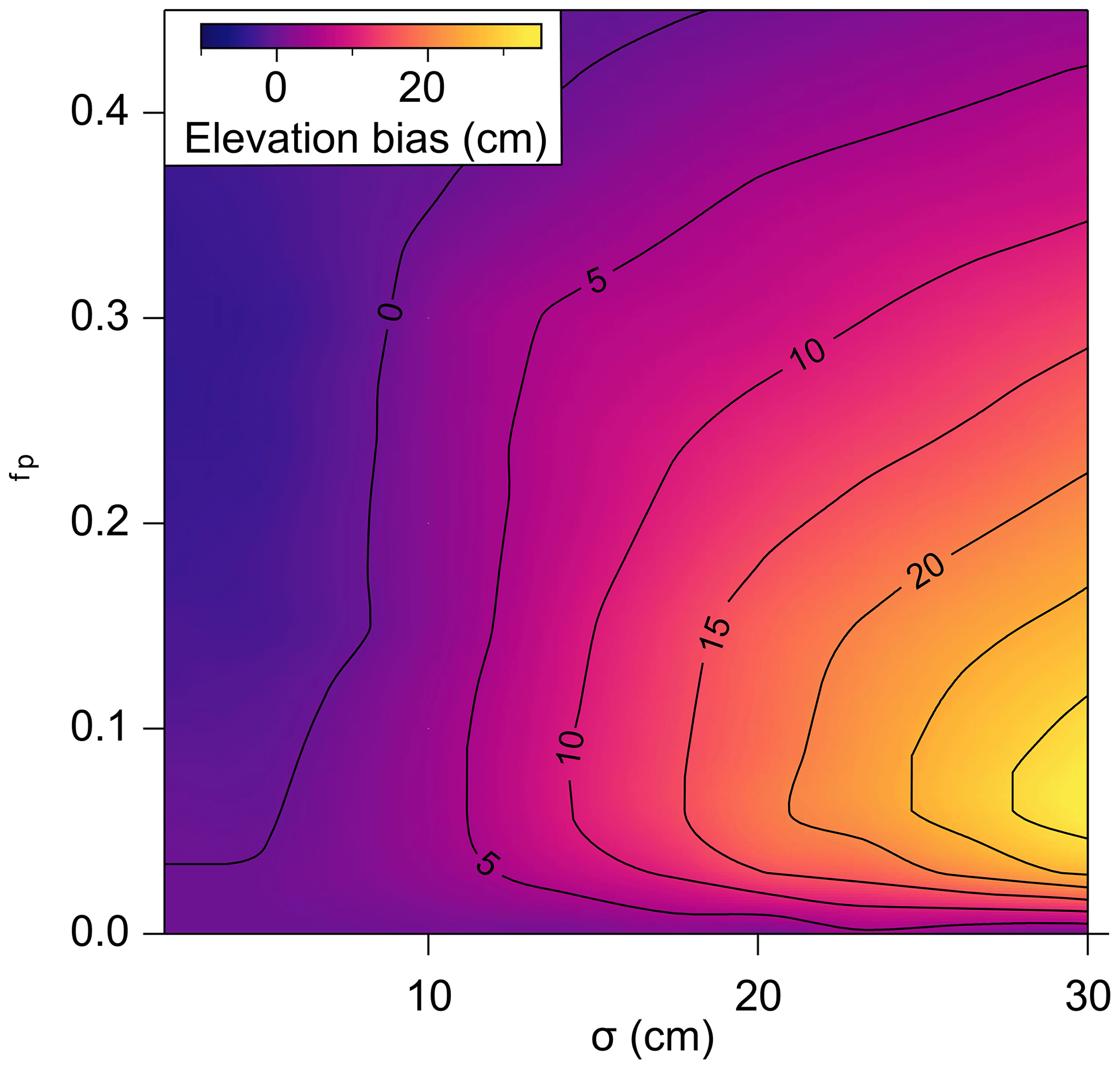
Figure 1 EM range bias for CryoSat-2 from Landy et al. (2022) as a function of surface roughness (σ) and melt pond fraction (f_p), created using a series of radar waveform simulations from a facet-based echo model (FBEM).

We calculate ice thickness in a similar way for a laser altimeter, where the sea ice freeboard is derived from the difference in elevations of leads and floes; however, the main difference is the sea ice floes measured by the laser references the top of the snow or bare ice surface. Over sea ice, the ICESat-2 satellite can also sample individual melt ponds and pressure ridges, as it has finer along-track sampling (0.7 m and a nominal 11 m diameter footprint, Magruder et al., 2021) compared to the along-track sampling of CryoSat-2 (∼300 m and a footprint size of $\sim \mathrm{300}\mathrm{m}\times \mathrm{1800}\mathrm{m}$). This enables us to better characterize surface roughness (Farrell et al., 2020) and investigate the laser reflectance behavior over individual melt ponds.

There have been several studies of ICESat-2 over summer sea ice. Farrell et al. (2020) demonstrated that we can use individual ICESat-2 ATL03 photon data to measure melt pond depth. The 532 nm (green) laser of ATLAS (Advanced Topographic Laser Altimeter System) can penetrate into clear water, and a portion of the reflected photons can therefore be returned from ice at the base of the pond, as well as its surface. This has been used more recently by Herzfeld et al. (2023) and Buckley et al. (2023) to analyze larger datasets over arctic sea ice to characterize melt pond depth. Tilling et al. (2020) investigated the photon scattering behavior over melt ponds by looking at observations coincident with WorldView-2 and Sentinel-2 imagery. They observed specular reflections over some melt ponds and leads; however, melt ponds with apparently higher water surface roughness or underlying ice surface roughness produce a lower reflectivity. The variability in backscatter, which can occur over the length of individual melt ponds, makes it challenging to determine the characteristics including height of melt ponds effectively. Additionally, this variability in pond reflectivity makes it difficult to classify leads from melt ponds, which is a vital step in calculating unbiased freeboard estimates.

Our ability to assess the performance and quantify any biases of experimental satellite-based summer sea ice freeboard products (and all ice thickness products) is limited by the scarcity of external validation data. To date, we have compared the CryoSat-2 summer sea ice thickness dataset (Dawson et al., 2022; Landy et al., 2022) with all available airborne Operation IceBridge Arctic summer campaigns, electromagnetic induction datasets (e.g., Alfred Wegener Institute (AWI) POLARSTERN ARK-XXVI/3 (TransArc) and IceBird campaigns), and mooring-based upward looking sonar (ULS) data (e.g., the Beaufort Gyre Exploration Program (BGEP) moorings). New observations will soon be available from the 2022 ICESat-2 Arctic Summer Airborne Sea Ice Campaign. All these data comparisons are either limited in time, with the airborne campaigns only spanning small and specific time periods, or limited spatially, with the buoy data only sampling specific locations. Additionally, these tend to be comparisons of ice thickness (or draft) and will therefore include additional uncertainties related to the conversion from radar freeboard to ice thickness, making it more challenging to assess any biases related to elevation retrieval. Uncertainties introduced in the conversion can come from errors in the assumed sea ice density, snow loading, surface meltwater loading, or EM bias correction (Landy et al., 2022).

On bare or melt-pond-covered ice, the ICESat-2 laser altimeter should be sampling the same surface as the CryoSat-2 radar altimeter. It is only over dry snow where we expect the two sensors to measure different floe heights, with the CryoSat-2 radar wave penetrating into snow, whereas the ICESat-2 laser measures the air–snow interface (Kwok et al., 2020c). However, over summer sea ice, ICESat-2 will not be susceptible to the EM bias that we observe in the radar altimetry data of CryoSat-2. Therefore, if we compare two coincident elevation measurements from CryoSat-2 and ICESat-2, the EM bias should be one (potentially major) component of the height difference, along with any other biases associated with either satellite. Additionally, in comparison to validations against small-scale in situ or airborne datasets, ICESat-2 has the spatial and temporal coverage to enable pan-Arctic full-summer intercomparison with CryoSat-2. To date, there have been several studies comparing ICESat-2 and CryoSat-2 over the Arctic Ocean in winter. Bagnardi et al. (2021) compared sea surface height anomalies (SSHAs) of several coincident tracks and found a mean difference of less than 3 cm. ICESat-2 and CryoSat-2 comparisons have also been used to investigate snow depth (Kwok et al., 2020c; Kacimi and Kwok, 2020), as the CryoSat-2 radar is assumed to reflect from the snow–ice interface, while ICESat-2 reflects off the air–snow interface. To our knowledge, this is the first study to compare ICESat-2 and CryoSat-2 over summer sea ice.

This study compares the height and reflectance statistics of the two sensors at crossover locations identified from the classification of CryoSat-2 observations as either ice floe or leads. This enables us to assess the performance of CryoSat-2, in particular the effect of different retrackers and characterization of the melt pond EM bias, against reference ICESat-2 observations. This does not assume that ICESat-2 sea ice elevations represent the “truth” during summer months, since ICESat-2 is susceptible to its own sources of bias; we simply characterize patterns of the elevation differences between sensors. At the time of writing, there was no reliable Level 3 ATLAS laser freeboard product publicly available for the summer months that can be used for a direct comparison between sensors. Thus, we will use the sea ice height (ATL07) and not the freeboard (ATL10) ICESat-2 data for comparison. There are several limitations to this study that should be stated at the outset. Although we are aiming to characterize the CryoSat-2 radar EM bias, any difference between CryoSat-2 and ICESat-2 we find will (at least partially) be due to unknown height biases in the CryoSat-2 and/or ICESat-2 data. In this context, we estimate which CryoSat-2 retracker has the best performance over melt-pond-covered ice. We also have no direct high-resolution measurements of the coverage of meltwater on the surface of the ice or of residual snow depth in summer, which impacts our ability to interpret any differences we find.

2 Data and methods

2.1 CryoSat-2 and ICESat-2 data processing

The CryoSat-2 satellite, launched in 2010, is equipped with the Ku-band (13.6 GHz) SAR/Interferometric Radar ALtimeter (SIRAL) instrument and uses either SAR or SAR interferometric (SARIn) altimeter modes over sea ice. The ICESat-2 satellite was launched in late 2018 and is equipped with a space-based lidar (Advanced Topographic Laser Altimeter System, ATLAS), with a wavelength of 532 nm. We used data from three summer seasons spanning May–September 2019–2021 while the satellites have been in orbit together.

We used CryoSat-2 ESA L1B and L2 baseline D data in this study, and we compared three different waveform retracking algorithms. (1) The results are provided in the ESA official L2 data product, which uses a threshold of the first peak for diffuse echo and a Gaussian plus exponential model fit for specular echoes, as described in Tilling et al. (2018). (2) The threshold first maximum retracker algorithm (TFMRA, Helm et al., 2014) is a threshold-based retracker applied to the waveform leading edge. This type of retracker has performed well over sea ice (e.g., Peacock and Laxon, 2004; Ricker et al., 2014). Threshold-based retrackers only consider the position of the center of the waveform (e.g., offset center of gravity, OCOG) or the location of the initial maximum (e.g., TFMRA) and can perform well when there is significant variation in waveform shape depending on the backscattering properties of the target surface. In particular, the TFMRA retracker has been used for retrieving sea ice freeboard over the winter months (Guerreiro et al., 2017; Kwok and Cunningham, 2015; Paul et al., 2018; Tilling et al., 2018). We calculate the TFMRA elevation data by retracking the ESA L1B waveforms and using a fixed threshold of 0.5 (TFMRA 50 %). Finally, (3) the SAMOSA+ physical retracker (Dinardo et al., 2018) is based on the SAMOSA2 delay-Doppler analytical radar echo model (Ray et al., 2014). This physical retracker is designed to account for a wide range of surface backscattering properties including quasi-specular and fully specular returns and measures the epoch, waveform power, significant wave height, and mean square surface slope. These data included zero-padding to increase waveform sampling, like the two other retracked datasets, but did not include a Hamming window filter. The Hamming filter step was included in the two other retracked datasets used in this study and is designed to reduce the effects of antenna side lobes on the returning waveform response. This could lead to a potential bias between the data, but it is likely to be small (Laforge et al., 2021). The CryoSat-2 SAMOSA+ data were processed using the SARvatore modules provided by the European Space Agency Grid Processing On Demand (G-POD) service (Dinardo et al., 2016)

We used the latest version (version 5) of the ATLAS/ICESat-2 L3A Sea Ice Height (ATL07) ICESat-2 data (Kwok et al., 2021), which are derived from the primary science Level 2A ATL03 data product. The L2A provides data for each of the three laser beam pairs from raw photon data with an along-track sampling interval of 0.7 m (with a nominal 11 m diameter footprint; Kwok et al., 2020c). The L3A along-track surface heights are measured by aggregating 150 geolocated signal photon heights, so the interval of the ATL07 data is reduced to between ∼30 and ∼75 m for the strong and weak beams, respectively (Tilling et al., 2020). The ATLAS instrument transmits laser pulses at 10 kHz and consists of three beam pairs separated by approximately 3 km. Each beam pair consists of a strong and a weak beam separated by 90 m, with the strong beam having approximately 4 times the transmitted energy. There are time-varying range biases between the beams that result in a centimeter-scale difference between the beams (Brunt et al., 2021). For example, there is roughly a 2–7 cm difference between the strong beams which is normally distributed about 0 m (Bagnardi et al., 2021). Thus, we compared each beam separately to the CryoSat-2 data.

ICESat-2 Sea Ice Height (ATL07) and CryoSat-2 (L2) products use different auxiliary data for calculating the surface elevation and satellite range corrections. The full table of corrections for both satellites can be found in the Bagnardi et al. (2021) supplementary information. ICESat-2 and CryoSat-2 use different mean sea surface (MSS) models: the CryoSat-2 MSS is compiled from CryoSat sea surface height measurements and CLS2011, while ICESat-2 uses a mean sea surface derived from CryoSat-2 data and DTU13 (Andersen et al., 2015; Kwok et al., 2020a). The satellites also use different tidal corrections (a combination of the FES2004 (finite element solution) tide model, Cartwright model, and Ssalto are used in the CryoSat-2 data, and a combination of the GOT 4.8 ocean tide model and International Earth Rotation and Reference Systems Service (IERS) 2010 conventions are used in the ICESat-2 data) and inverse barometer corrections (CNES Ssalto (ECMWF) and NASA Global Modeling and Assimilation Office (GMAO) GEOS-5 Forward Processing for Instrument Teams (FP-IT) for CryoSat-2 and ICESat-2, respectively) to calculate surface elevation. Bagnardi et al. (2021) found that the different inverse barometer corrections led to an average difference of 2.6 cm, while tide values and other geophysical corrections have a mean difference of <0.3 cm between sensors. We do not correct for the differences in tide values, inverse barometer corrections, and other geophysical corrections in this analysis, so there will be an additional source of uncertainty up to around ±3 cm. We do, however, replace the MSS used in the CryoSat-2 data with the one used in the ICESat-2 data processing chain by bilinearly interpolating MSS values from a 2.5 km grid. The interpolation will produce a small error in retrieved CryoSat-2 heights; however, this will be negligible from such a dense 2.5 km grid. All three different CryoSat-2 elevation datasets, from each retracking algorithm, were processed with the same corrections.

We also used several parameters related to the reflectivity of the sea ice surface (which can indicate the presence and coverage of surface water on the ice), along with elevation information, to interpret the height differences observed between sensors. We included the ICESat-2 photon rate (N_photons), which is the number of detected photons divided by the number of laser shots required to construct the 150-photon aggregate. This gives a measure of the apparent surface reflectance; however, it is affected by the presence of clouds, as they can attenuate the strength of surface returns. Thus, we only included this parameter when all data had a high confidence of being cloud free using the “cloud_flag_asr”. Note that the cloud cover flag is sampled every 400 m along track (Kwok et al., 2020b). Thus, some values of photon rate that are cloud free will be omitted, while we may include some points contaminated by clouds. We also included the CryoSat-2 backscatter coefficient (σ⁰), which is a calibrated measurement of the normalized backscatter cross-section of the return radar pulse. There is currently no lead flag in the ICESat-2 ATL07 data over the summer months. Thus, we used the summer lead detection scheme in Dawson et al. (2022) to classify CryoSat-2 observations and apply the same classification to coincident ICESat-2 observations. This classifier uses variations in along-track parameters to distinguish between leads and floes in the summer, overcoming the limitations of other classifiers which perform poorly when reflections from most surfaces are specular (e.g., Lee et al., 2018). Using this scheme in this context is limited. The summer classifier is known to classify significantly fewer leads compared to the winter classifier due to the increased noise in the summer data, caused by highly reflective melt ponds causing off-nadir snagging. Snagging occurs when the surface has heterogenous backscattering properties at a smaller scale than the radar footprint, causing the radar return to be dominated by the most reflective portion of the footprint, at or outside the nadir point. This will not impact comparison of the lead elevation data; however, there will be a proportion of misclassified leads in the ice floe elevation data. Additionally, as we are comparing one CryoSat-2 point to multiple ICESat-2 points (see “Satellite crossover locations”), we are likely to compare the CryoSat-2 lead elevation to a mixture of ICESat-2 lead and floe elevations, as not all ICESat-2 points will sample the lead location. This is compounded by the fact that along-track location of the leads can be incorrect in location by up to one sample along track due to how the classification scheme works, and therefore we may not be sampling the lead location at all in the CryoSat-2 data as well. In the early and late summer, there could still be a significant snow cover on Arctic sea ice floes. This is supported by the lower CryoSat-2 backscatter and ICESat-2 photon counts observed in the early and late summer (see Fig. 5), inferring that there is snow on the surface of the sea ice or at least the surface is not covered in more reflective melt ponds. Thus, we only used observations from 9 July to 16 August because these times had consistently higher CryoSat-2 backscatter and ICESat-2 photon counts than the transitions periods between spring–summer and summer–fall. The SARIn mode is limited to the coastal regions during our study period and was not used in this comparison.

2.2 Additional datasets

We used melt pond fractions (f_p) derived from the Sentinel-3 Ocean and Land Colour Instrument (OLCI) data version 1.5 by Istomina (2020). This dataset is provided by the University of Bremen and is produced on a daily 12.5 km grid. Melt pond fraction is only available over cloud-free pixels, and, to ensure a complete daily grid, we calculated the average melt pond fraction over each grid cell within a 15 d window of the altimeter samples, weighted by a tri-cube weight function (i.e., $(\mathrm{1}-([t_{\mathrm{d}}/t_{\mathrm{m}}]{)}^{\mathrm{3}}{)}^{\mathrm{3}}$, where t_d is time from measurement point, and t_m=7.5 d). We also used sea ice drift observations from Polar Pathfinder Daily 25 km EASE-Grid Sea Ice Motion grids (Tschudi et al., 2022) and daily sea ice age data EASE-Grid Sea Ice Age, Version 4 (Tschudi et al., 2022) 12.5 km grids. We obtained the melt pond fraction, sea ice drift speed, and sea ice age data at each crossover location by linear interpolation from each EASE grid.

2.3 Satellite crossover locations

ICESat-2 and CryoSat-2 intersections were found using the cs2eo (Ewart et al., 2022) coincident data explorer. This platform was created as part of the CRYO2ICE campaign, where CryoSat-2 and ICESat-2 were periodically aligned, enabling along-track analysis between the two sensors. Unfortunately, the time difference between the two satellites for the CRYO2ICE orbits are more than 3 h apart, and this was beyond the minimum we required in this study (see below). However, the data explorer was a valuable resource for finding coincident data.

We compared CryoSat-2 and ICESat-2 elevation data using a “point-to-points” crossover methodology, where we compared one CryoSat-2 footprint to multiple ICESat-2 sampling points within a 150 m radius. This ensured that we sampled approximately the exact same surface, and we did not include any interpolation from neighboring data in the comparison, which may introduce additional uncertainties. We used the mean of multiple ICESat-2 points to leverage its higher resolution and increase precision of the ATL07 data. The 150 m radius allowed us to compare the ice surface over the length scales of the CryoSat-2 SAR mode along-track footprint of ∼300 m. We treated each ICESat-2 beam separately and calculated individual crossovers for each beam. We only compared data where CryoSat-2 footprints contained at least 50 coincident ICESat-2 measurements. We also calculated the root mean square (RMS) height difference of the ICESat-2 points within this radius to obtain a measure of the surface roughness (σ_IS2).

Sea ice drift means that any intersection locations can separate over time, and hence we can only compare data within a short time of each other. Crossovers close together in time typically occur at the maximum inclinations of the orbits (see Fig. 2). In this region (above 80^∘), the typical average ice drift velocity is 130 m h⁻¹, based on the Polar Pathfinder dataset. To ensure that we are sampling approximately the same locations, we only used points within 3 h and which had drifted less than 300 m based on sea ice drift observations. Given the spatial and temporal resolution of the Polar Pathfinder Daily 25 km EASE-Grid Sea Ice Motion grids, we could only obtain a rough estimate of drift speed, and thus we included the 3 h maximum time limit as well to account for this, even when ice drift was very low and in theory pairs could be obtained at longer time differences. Using this method, we removed data where footprints had clearly drifted apart whilst retaining as much data as possible when ice drift speeds were low. Despite including these constraints, longer time differences between coincident measurements result in larger deviations between CryoSat-2 and ICESat-2 elevation data, meaning that ice drift will affect the final comparison. For example, comparing CryoSat-2 and ICESat-2 elevation data within 90 min and data between 90 and 120 min, the median absolute deviations (MADs) are 0.075 m (84 % of observations) and 0.087 m (16 % of observations), respectively. We could reduce the maximum time between intersections to reduce the impact of ice drift; however, we decided on a maximum 3 h time difference and 300 m drift as a compromise between accuracy and the availability of as much data as possible for comparison.

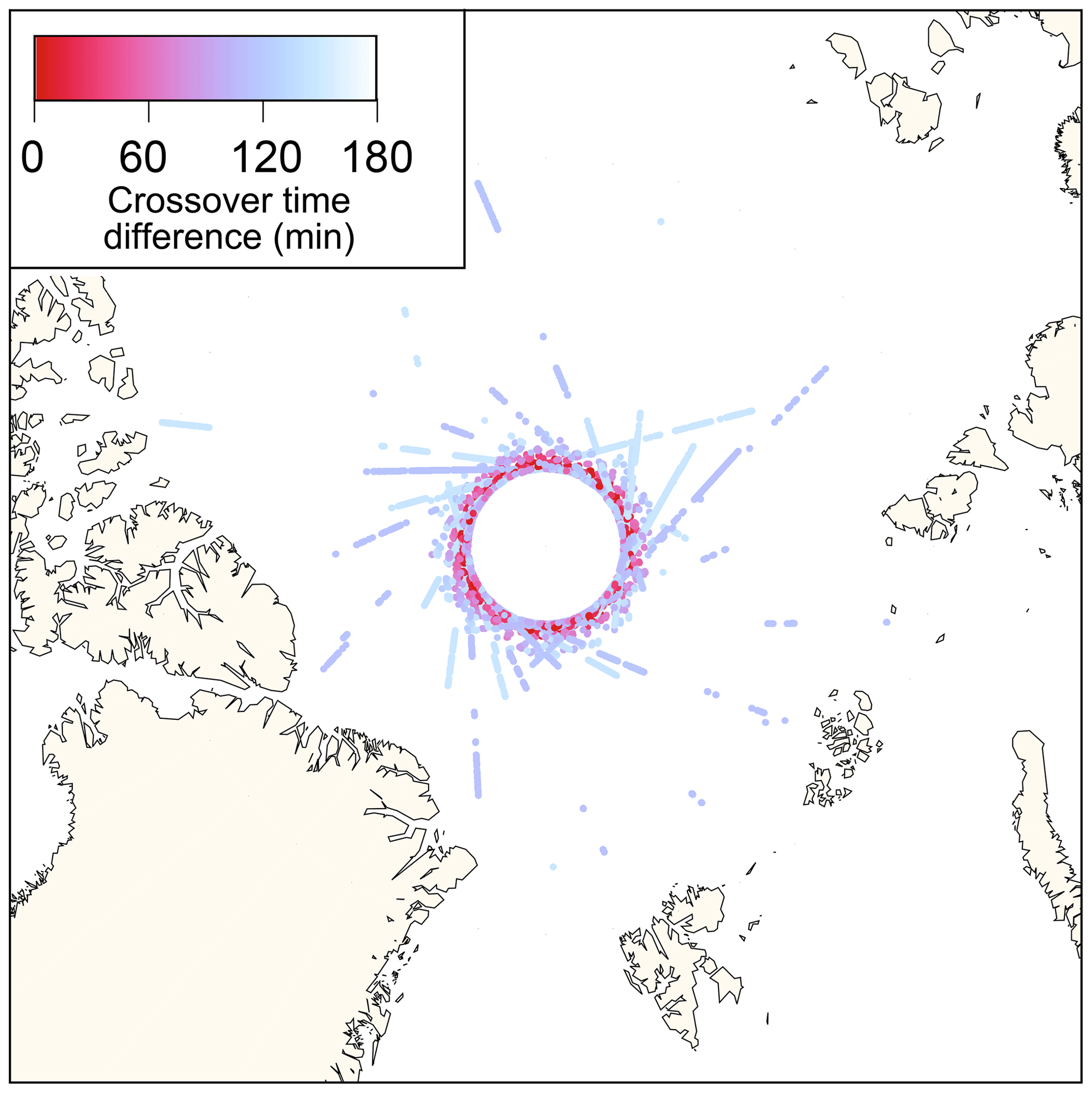
Figure 2 CryoSat-2 and ICESat-2 crossover locations and time difference between intersections for data up to 3 h apart.

3 Results

3.1 Comparison of CryoSat-2 surface elevation retracking algorithms

Overall, we obtained 60 775 coincident measurements for comparison in July–September across the period between 2018 and 2021. These data are typically located near the maximum inclination of the CryoSat-2 and ICESat-2 orbits in the central Arctic Ocean (see Fig. 2). Distributions of the elevation differences between ICESat-2 and CryoSat-2 are shown in Fig. 3 for the different retracking algorithms used in this study and all ICESat-2 beams combined. For all retrackers, the CryoSat-2 elevation measurements are generally lower than ICESat-2 by a median difference of 7.1, 1.6, and 2.4 cm for the ESA L2, TFMRA, and SAMOSA+, respectively. We used median differences to reduce the effects of outliers on the measurements. The distributions are non-Gaussian and are positively skewed. This implies that there are non-linear differences between the surface heights recorded by each sensor, and the tail of the distribution is contributing to the difference. This is discussed in greater detail later in this section. All retracked elevation differences have a similar median absolute deviation (MAD) of 5.4, 4.3, and 5.0 cm for the ESA L2, TFMRA, and SAMOSA+ retrackers, respectively. Hereafter, we use the SAMOSA+ retracked elevation difference for comparison because this is the retracking algorithm used for our existing summer sea ice freeboard and thickness retrievals (Dawson et al., 2022; Landy et al., 2022).

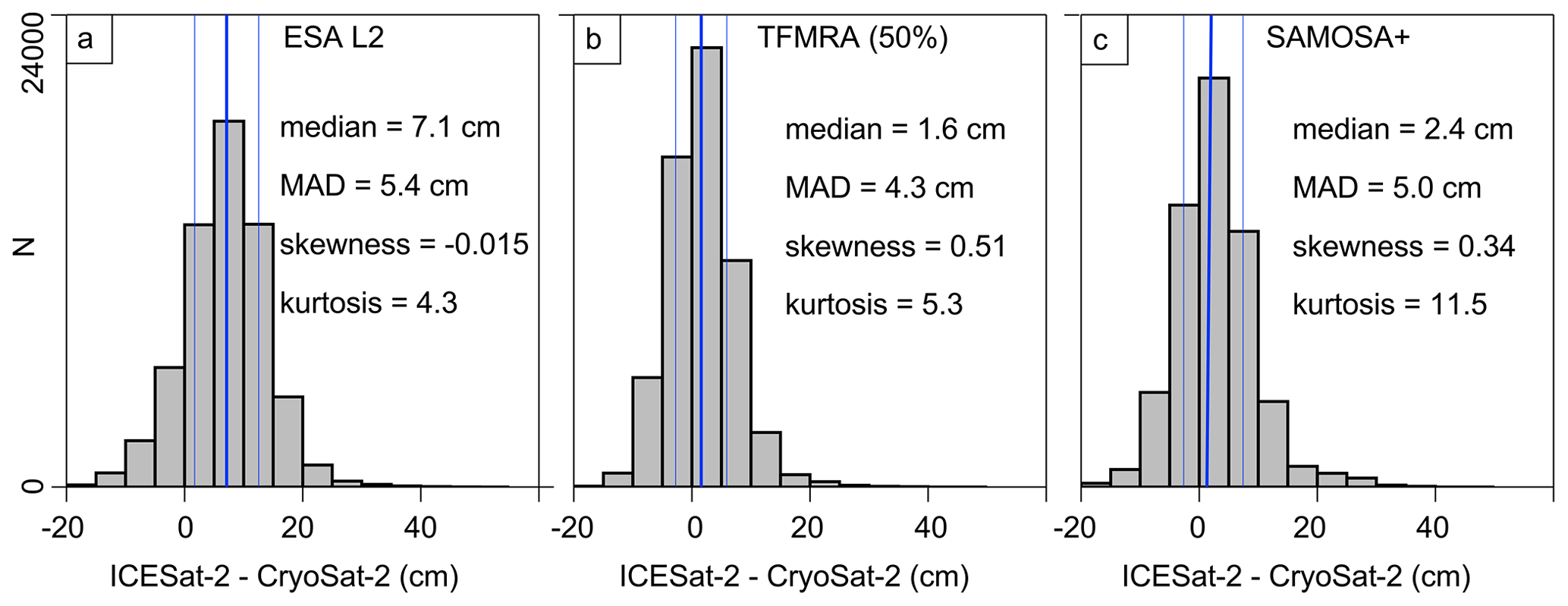
Figure 3 Distributions of ICESat-2 elevation minus CryoSat-2 elevation for the (a) ESA L2, (b) TFMRA (50 %), and (c) SAMOSA+ CryoSat-2 retrackers at orbit crossover locations.

As a result of most of the crossovers being at the maximum inclination of the satellite orbits, the majority (80 %) of the data were sampled over sea ice with an age greater than 1 year. The median difference between ICESat-2 and CryoSat-2 ice was 1.3 and 2.5 cm, while the MAD was 7.6 and 4.7 cm for the first-year and multi-year ice, respectively (Fig. 4).

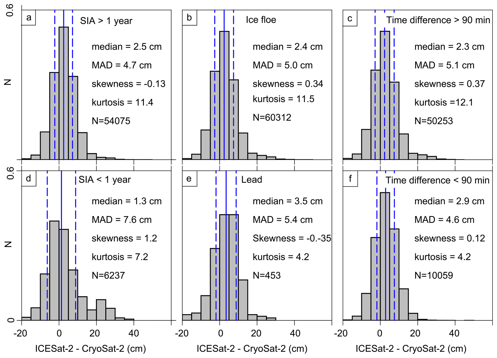
Figure 4 Distributions of ICESat-2 minus CryoSat-2 SAMOSA+ for sea ice age (SIA) < 1 year (a), SIA > 1 year (d), data classified as leads (e), data classified as floes (b), within 90 min of coincident measurements (f), and greater than 90 min of coincident measurements (c).

We only classified 0.75 % (453 points) of the data as leads; however, the true number of leads within our dataset of paired samples is likely to be higher, as the classification method used is conservative and is known to omit valid leads (Dawson et al., 2022). The CryoSat-2 elevation measurements at leads are lower than ICESat-2 by a median difference of 3.5 cm (5.4 cm MAD). Most pairs were sampled within 90 min (84 %), and these samples had a lower variability with a median difference and MAD of 2.9 and 4.6 cm, respectively, compared to the data with a time difference greater than 90 min and with a median difference and MAD of 2.3 and 5.1 cm, respectively.

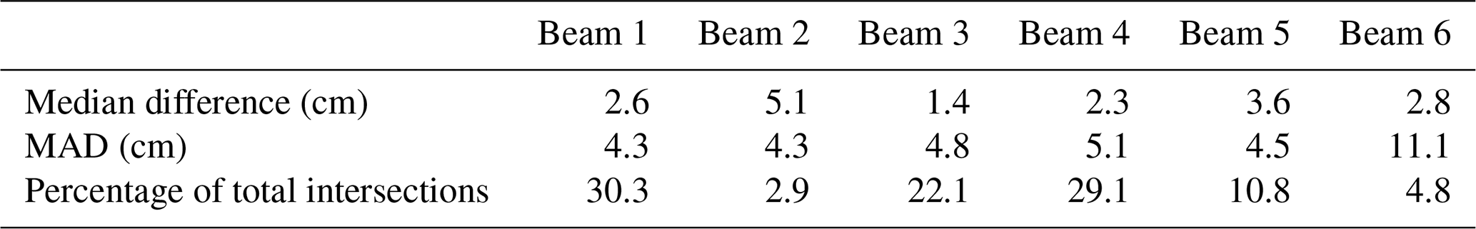
The comparison with individual beams of ICESat-2 is shown in Table 1. The median difference between ICESat-2 beams and CryoSat-2 elevations ranged from 1.4 to 5.1 cm, which is in the range of the bias observed between beams by Bagnardi et al. (2021). Beams 2 and 6, which are weak beams and had significantly fewer crossovers with CryoSat-2, had the largest median difference (beam 2) and MAD (beam 6). If we compare the difference between the weak and the strong beams of ICESat-2 and CryoSat-2, we find a median difference of 2.5 and 2.3 cm and MAD of 5.8 and 4.5 cm, respectively. This is not a direct comparison between beams because the points being sampled for each beam are at different locations and may be over different ice conditions.

Table 1 Median difference and median absolute difference (MAD) between CryoSat-2 and the six individual beams of ICESat-2. Beams 1, 3, and 5 are the strong beams.

3.2 Relationships of height offsets to sensor backscatter, reflectance, and surface roughness

To examine whether sea ice properties cause the distributions of elevation differences between CryoSat-2 and ICESat-2 to be non-Gaussian positively skewed, we examine photon rate and roughness from ICESat-2 and the backscatter coefficient from CryoSat-2. We expect a higher photon rate and radar backscatter at nadir look angles from smooth, reflective surfaces such as melt ponds (Kwok et al., 2019). Therefore, we might expect the pan-Arctic average reflectance and backscatter to increase with the formation and expansion of melt ponds, then decline with their drainage later in summer. We observe this relationship if we look at the evolution of the photon brightness and radar backscatter through the summer months (see Fig. 5), with higher values in the mid-summer months of July and August when melt ponds are generally at their peak (Rösel et al., 2012). Towards the start and end of the summer, we observe more variability in the CryoSat-2 backscatter (with a MAD of 3.2 dB for points from the 9 July to 16 August compared to 7.7 dB for points before 9 July and after 16 August) when there is snow covering the sea ice, with variable temperatures and melting states, or as melt ponds freeze at the seasonal transitions. The ICESat-2 photon rate displays similar variability throughout the summer, with a MAD of 1.4 for points between the 9 July and 16 August and 1.9 for points before 9 July and after 16 August. This is because melt ponds can vary in reflectivity depending on the water surface roughness (Tilling et al., 2020) and their coverage on the ice surface changes. We also see this seasonal pattern if we compare to the evolution of melt pond fraction from Sentinel-3 OLCI data, with the highest melt pond fractions being from mid-July onwards. For all other data used in this study, the time range was constrained between observations from 9 July to 16 August.

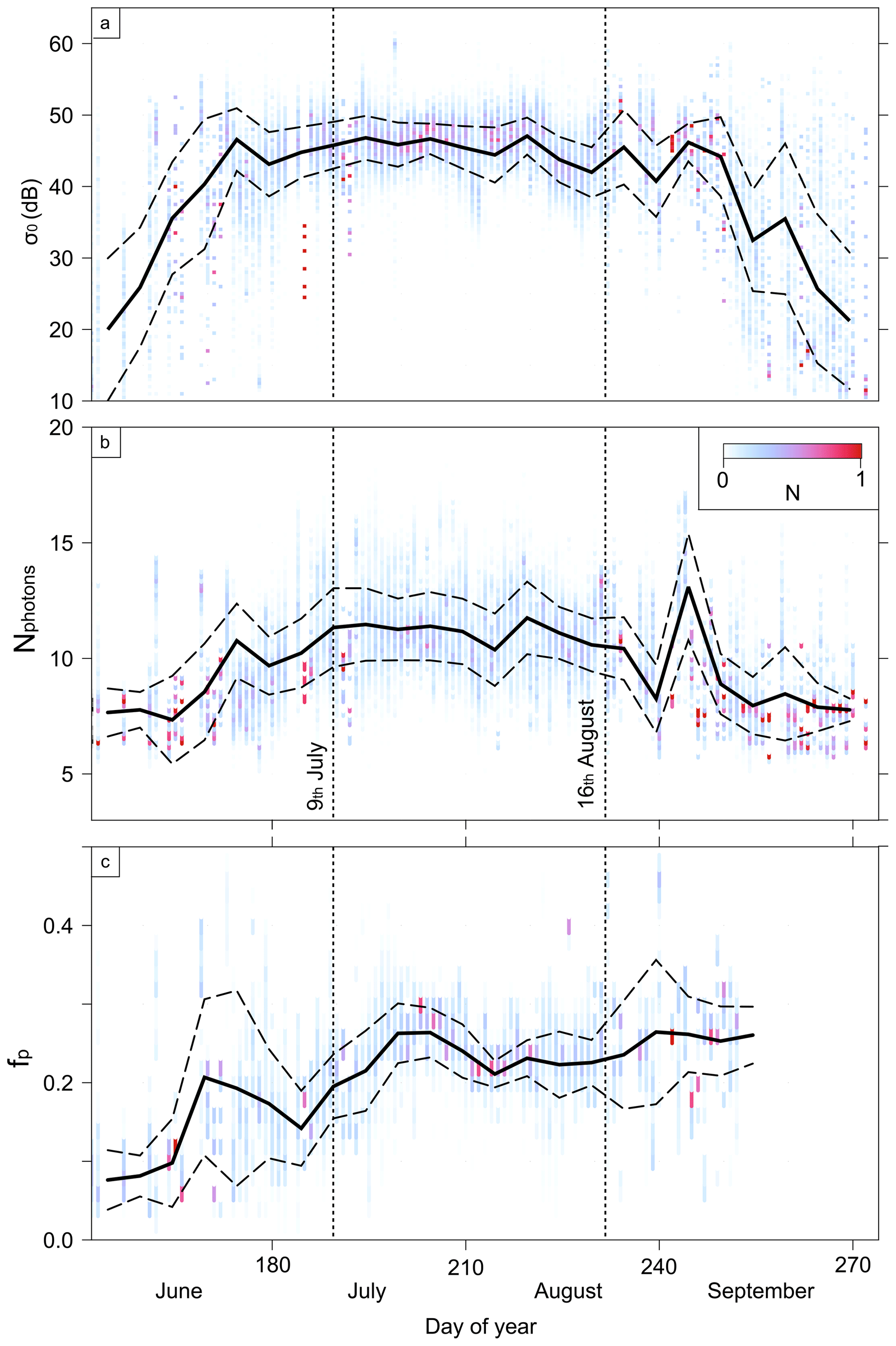
Figure 5 (a) Median CryoSat-2 backscatter (σ⁰), (b) ICESat-2 photon rate (N_photons), and (c) Sentinel-3 OLCI melt pond fraction (f_p) for the day of year (black line) over the 3-year study period (2018–2021) for all crossover points. The vertical lines displaying 9 July and 16 August show the data used in the rest of study. The background points display the distribution of measurements for each day, while the dashed lines show the median absolute deviation of these points.

There is also a positive relationship between ICESat-2 photon rate and CryoSat-2 backscatter for both the strong and weak beams (Fig. 6). The data are scattered; however, we observe that low backscatter and low photon rates tend to be from rougher surfaces. This is particularly apparent in the strong beam comparison, where the highest surface roughness (σ_IS2>0.2 m) observations have backscatter and photon rates lower than 45 dB and 7, respectively.

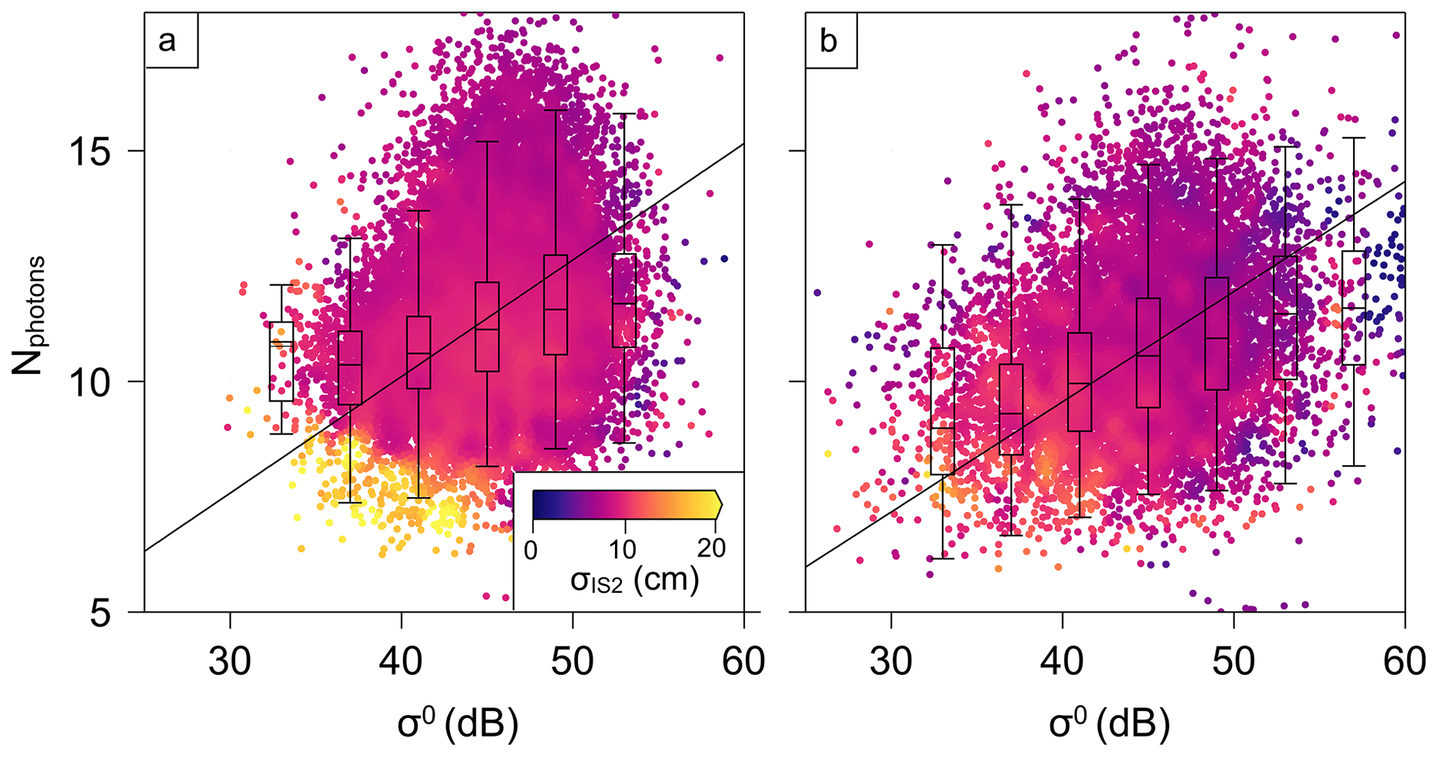
Figure 6 ICESat-2 photon rate (N_photons) vs. CryoSat-2 backscatter (σ⁰) for the (a) strong and (b) weak beams of ICESat-2, along with a line of best fit. The color of each point is the surface roughness (measured using the RMS of the surface measured by ICESat-2 within a 150 m radius), which is smoothed using a 5×5, _P×σ⁰ kernel. The box plots represent the 2nd, 25th, 50th, 75th, and 98th percentiles of the binned data.

CryoSat-2 elevations are increasingly lower than the ICESat-2 elevations over rougher ice, as seen in Fig. 7a; however, the data are scattered, meaning there is not a significant relationship between the two parameters at the CryoSat-2 footprint scale. The least-squares fit between the altimeter elevation difference and roughness has a slope of 0.659 ± 0.007 cm cm⁻¹; i.e., the range bias increases by 3.2 cm for every 5 cm the sea ice surface roughness increases. At the minimum measured sea ice surface roughness of ∼3 cm, the range bias is 1.9 cm according to the line of best fit, suggesting that the bias is very small – close to zero – for smooth, level sea ice floes. For a roughness of 15 cm, at the upper end of the measured roughness distribution, the range bias is 9.9 cm according to the line of best fit. This difference is reinforced by the comparison between first-year and multi-year ice, where CryoSat-2 underestimates elevation more over rougher multi-year ice than smoother first-year ice (Fig. 2). Although we cannot be sure that the absolute offsets between the two sensors are not affected by other sensor biases, the relative height offsets for smoother and rougher sea ice observed in Fig. 7a are likely to be caused by the EM bias discussed in the introduction.

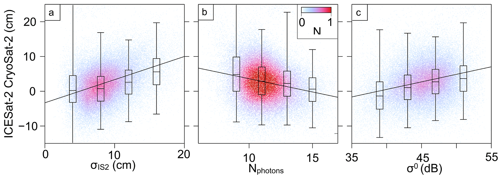
Figure 7 Elevation difference between ICESat-2 and CryoSat-2 vs. (a) surface roughness (RMS of the surface measured by ICESat-2 within a 150 m radius σ_IS2), (b) ICESat-2 photon rate (N_photons), and (c) CryoSat-2 backscatter (σ⁰). Each plot displays a line of best fit; due to the number of points, individual points are not plotted, but instead we display the point density. The box plots represent the 2nd, 25th, 75th, and 98th percentiles of the binned data.

3.3 Melt pond bias

Both the surface backscatter/photon rate and the surface roughness are related the magnitude of elevation differences between the laser and radar altimeters. To investigate this further, we explored the relationships between melt pond fraction, surface roughness, and elevation differences, as shown in Fig. 8b and c. Here we observe that the largest elevation differences occur over rougher surfaces with relatively low photon rate and backscatter, inferring that ice floes with a lower coverage of surface water produce a larger height difference. We can investigate how this bias is related to the theoretical predictions in Fig. 1 by plotting the surface roughness vs. melt pond fraction (from external Sentinel-3 OLCI data) in Fig. 8a, with the color of the marker representing the elevation difference between ICESat-2 and CryoSat-2. As the data are scattered, we smoothed the elevation differences on the figure using a 0.01$/$1 cm $f_{\mathrm{p}}/{\mathit{\sigma }}_{\text{IS2}}$ kernel. The observations are overlaid onto contours showing the theoretical EM range bias obtained from radar waveform simulations, as described in Landy et al. (2022) and illustrated in Fig. 1.

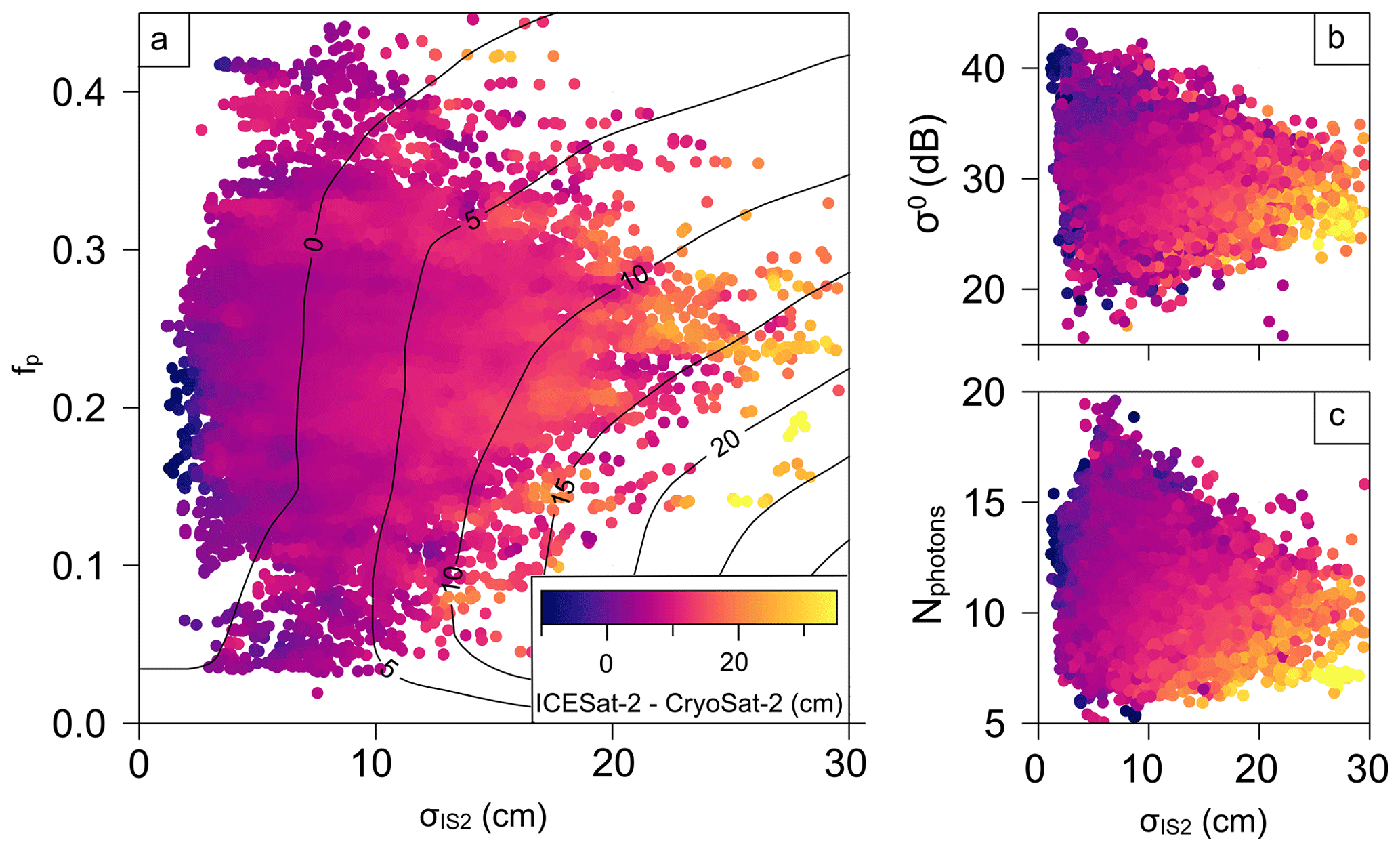
Figure 8 Elevation difference between ICESat-2 and CryoSat-2 as a function of (a) melt pond fraction (f_p) and surface roughness (σ_IS2), (b) CryoSat-2 backscatter rate (σ⁰) and surface roughness (σ_IS2), and (c) photon rate (N_photons) and surface roughness (σ_IS2). The melt pond fraction is derived from Sentinel-3 OLCI data, while the surface roughness is the RMS of the surface measured by ICESat-2 within a 150 m radius. The background contours on the left plot illustrate the theoretical radar freeboard bias derived from model simulations in Landy et al. (2022). The elevation differences are smoothed with a 1 cm$/$1, 1 cm$/$5 dB, and 1 cm$/$5, ${\mathit{\sigma }}_{\text{IS2}}/f_{\mathrm{p}}$, ${\mathit{\sigma }}_{\text{IS2}}/{\mathit{\sigma }}^{\mathrm{0}}$, and ${\mathit{\sigma }}_{\text{IS2}}/N_{\text{photons}}$ kernel, respectively.

The melt pond fractions derived from OLCI data have a spatial and temporal resolution several orders of magnitude lower than the collocated footprint samples of the altimeters (i.e., 12.5 km grid interpolated over a 15 d period) so will not give a precise indication of the surface properties at the exact location of the footprint. Despite this, after smoothing the roughness signal, the magnitudes of the observed ICESat-2- CryoSat-2 elevation differences follow very similar patterns to the theoretical EM range bias obtained from model simulations (which varied from around 0–30 cm). When the melt pond fraction is high (20 %–30 %), the elevation difference is around 5–10 cm regardless of the sea ice surface roughness. When the pond fraction is lower (f_p<20 %), the elevation difference increases significantly from 0 up to 30+ cm when the sea ice surface roughness increases (Fig. 8a). Very few points were sampled that had low melt pond fraction (f_p<10 %) and high surface roughness (σ_IS2>30 cm), where we obtain the largest biases in the theoretical predictions. However, the pairs with the lowest melt pond fraction (f_p<20 %) measured at high roughness (σ_IS2>20 cm) had the largest height offsets observed within our dataset. We also observe the same relationship when we plot the altimeter elevation difference and sea ice surface roughness as a function of the CryoSat-2 backscatter and ICESat-2 photon rate (Fig. 8b and c). As discussed previously, the backscatter and photon rate are not direct measurements of melt pond fraction but can indicate the presence or absence of melt ponds, and their relative coverage, and are measured directly from the satellite

4 Discussion

4.1 Comparison with previous work

CryoSat-2 generally records lower-elevation measurements of lead and sea ice surfaces compared to ICESat-2 during the Arctic summer months of July–September. This is consistent when the CryoSat-2 elevation observations are processed with three different retracking algorithms. This phenomenon has been observed before when CryoSat-2 summer sea ice freeboards were compared to ice freeboard, thickness, and draft observations recorded by independent airborne and in situ instruments (Dawson et al., 2022). However, previous comparisons to sea ice draft or thickness in the summer include additional uncertainties relating to the sea ice densities assumed for converting freeboard to thickness. Therefore, the most relevant independent comparisons to this work were made between CryoSat-2 radar freeboards and the laser freeboards recorded by Operation IceBridge during two campaigns over mid-summer sea ice (when snow is assumed to be absent from the ice surface). The Operation IceBridge Arctic summer campaigns operated in the Chukchi Sea on 16 and 19 July 2016 and the Lincoln Sea on 24 and 25 July 2017. The radar freeboards derived from CryoSat-2 elevation data using the SAMOSA+ retracker underestimated the IceBridge Airborne Topographic Mapper (ATM) laser freeboards by between 2–20 cm (Dawson et al., 2022). For the thicker multi-year sea ice freeboards in the Lincoln Sea, the freeboards were underestimated by 10 ± 6 cm and 20 ± 10 cm below and above an arbitrary roughness threshold of 35 cm, which highlights a similar relationship with surface roughness to the comparisons in this study. Recently acquired airborne observations from the 2022 ICESat-2 Summer Sea Ice Campaign, including for CRYO2ICE orbits, will enable further independent validation of both satellite sensors over melting sea ice.

We observe a difference of 2 ± 5 cm between ICESat-2 and CryoSat-2 using the SAMOSA+ retracker. The data are not exactly comparable, as the IceBridge flights were made over the Chukchi Sea and the Lincoln Sea and include the conversion from elevation to freeboard, rather than the simple elevation-to-ellipsoid comparison between CryoSat-2 and ICESat-2 made at central Arctic crossovers here. The negligible height differences obtained here between CryoSat-2 and ICESat-2, compared to the height differences between CryoSat-2 and the IceBridge ATM even over smoother sea ice, suggest that ICESat-2 ATL07 sea ice heights may also be underestimating the true sea ice floe surface elevation. This could indicate that there is a bias associated with the ICESat-2 height retrieval over melt ponds. However, previous work has suggested that the ATL03 ICESat-2 elevation data would likely be biased high, as highly reflective surfaces (such as melt ponds) may cause saturation of the ATLAS detector, preventing it from recording all the recorded photons, with the photons on the leading edge of the returns being preferably sampled (Tilling et al., 2020). However, there could be other important processes affecting the ICESat-2 photons. For example, the roughness of melt pond surfaces could affect a bias in the retrieved mean elevation, or penetration of the laser through the meltwater may produce a final elevation that is a mixture of the pond surface and bottom. Given that we observed a significant height offset over leads (where we do not expect a radar EM range bias) as well as ice floes, the absolute height offsets between CryoSat-2 and ICESat-2 over sea ice have to be interpreted carefully. Ideally, we could use the offset at lead locations to quantify any other biases associated between the two satellites not related to melt ponds. However, as stated earlier, we are likely comparing a mixture of both lead and floe elevations, and therefore we cannot reliably obtain a bias that is obtained just from leads.

Each of the CryoSat-2 retrackers generally recorded lower elevations compared to coinciding ICESat-2 observations; however, ESA L2 had the greatest difference. Additionally, the MAD is smaller for the SAMOSA+ and TFMRA retrackers compared to the ESA L2 results, and while we cannot determine the overall performance of each retracker because of the uncertainty related to the ICESat-2 data, the results suggest that SAMOSA+ and TFMRA retrackers perform more consistently over both specular and diffuse reflecting surfaces. We used a 50 % threshold for the TFMRA retrackers, which has commonly been used for sea ice studies (e.g., Ricker et al., 2014); however, a lower threshold giving a shorter range estimate could reduce the bias observed between ICESat-2 and CryoSat-2 further. This will not remove the EM bias observed in the CryoSat-2 data because the height difference distributions are clearly non-Gaussian and positively skewed, indicating that the EM bias varies non-linearly as a function of the sea ice surface properties.

4.2 Comparison with theoretical predictions

The theoretical bias (see Fig. 1) calculated by Landy et al. (2022) behaves similarly to our observations comparing CryoSat-2 with ICESat-2 data. We can see this in Fig. 8, where there is an increase in bias for lower melt pond fraction data at a given surface roughness. Unfortunately, we do not obtain a large range of melt pond fractions from our sample of coinciding measurements at crossovers, with the majority of pond fractions above f_p=0.1, so it is challenging to compare the empirical and theoretical biases at low melt pond fractions. This is limited by our restriction to the mid-summer July–August study period when surface conditions are more stable but removes data from the early summer when pond fractions are smaller. Despite this limitation, the bias increases as the surface gets rougher (Fig. 3b) and, for a given roughness, is larger for surfaces with lower reflectivity (Fig. 4). However, we find that the empirical data show larger biases (5–10 cm) for relatively lower roughness (σ_IS2<10 cm) when compared to biases resulting from the theoretical simulations (0–5 cm).

Additionally, the highest biases observed from the empirical data (20–35 cm) are in the region where theoretical simulations suggest they should be highest (i.e., higher surface roughness but lower melt pond fraction/photon rate). However, the theoretical biases in this region are lower (10–20 cm) than those observed in the experimental data. It is not possible with the data available in this study to determine the likely source of any additional bias or difference between experimental observations and theoretical predictions. We require a deeper understanding of the interactions between both laser and radar altimeter sensors with the summer sea ice surface to better understand the radar EM bias. More in-depth studies from airborne underflights of each sensor, during the Arctic summer months, could improve this understanding, for instance by interpreting the specific reflectance and backscattering properties in “known” conditions with detailed reference data. The theoretical work (Landy et al., 2022) and experimental observations here provide a starting point for designing such airborne studies. They should target the relationships between melt pond properties (roughness, melting state, coverage), sea ice floe surface roughness, and the radar/laser waveform characteristics they produce.

5 Summary

We compared coincident CryoSat-2 and ICESat-2 elevation measurements over Arctic summer sea ice between 2018 and 2021. The intersections were based on the CRYO2ICE orbits, and we compared one CryoSat-2 data point to multiple ICESat-2 points within a 150 m radius, owing to the higher resolution of the ICESat-2 satellite. We found that CryoSat-2 records a lower elevation compared to ICESat-2, and distributions are non-Gaussian and positively skewed. The bias ranges from 0.071 (5 % percentile) to 0.135 (95 % percentile) for the SAMOSA+ retracked CryoSat-2 elevation data. The median bias ranges between 1–3.5 cm and is observed when we compare individual ICESat-2 beams and use different retrackers on the CryoSat-2 waveform data.

The observed bias between CryoSat-2 and ICESat-2 is likely due to melt ponds in the surface of the ice, lowering the principal scattering horizon of the radar pulse. This has been observed and modeled in other studies (Dawson et al., 2022; Landy et al., 2022) and theoretically shown to be dependent on the melt pond fraction and the surface roughness. We were able to measure the surface roughness from the ICESat-2 data, and while the increased reflectivity of the surface to the radar and laser altimetry may indicate the presence of melt ponds on the surface of the ice, we have not yet determined an accurate measure of the melt pond fraction from either altimeter directly. Gridded melt pond fraction data derived from Sentinel-3 OLCI were too low resolution to be used for interpreting height biases at individual crossover locations. Despite this, we observed a similar pattern between ICESat-2 surface roughness, OLCI melt pond fraction, and the altimeter height bias as predicted by theoretical waveform simulations. However, the observational data had larger biases between 5–10 cm for surface roughness σ_IS2<0.1 m when compared to biases of 0–5 cm resulting from the theoretical simulations. This could be due to other biases relating to the comparison of absolute elevation measurements between sensors.

This is the first experimental investigation of the melt pond bias, and future studies should use the ICESat-2 data to aid our theoretical understanding and improve the corrections needed when using radar altimetry data over sea ice. Equally, the intercomparison can improve our understanding of ICESat-2 laser altimetry returns over summer sea ice, which suffer from their own biases and challenges related to melt ponds. This will, in turn, improve summer sea ice thickness products obtained from both sensors. Improved high-resolution observations of melt pond fraction (and to a less extent surface roughness) are now needed to apply bias corrections to radar altimetry data over summer sea ice. Airborne-satellite underflights are also needed to improve our theoretical understanding of the radar EM bias and to validate updated summer sea ice freeboard retrieval algorithms.