the Creative Commons Attribution 4.0 License.
the Creative Commons Attribution 4.0 License.
 | 31 Jan 2023
Modulation of the seasonal cycle of the Antarctic sea ice extent by sea ice processes and feedbacks with the ocean and the atmosphere
Sofia Allende Contador
Cecilia M. Bitz
Edward Blanchard-Wrigglesworth
Clare Eayrs
Thierry Fichefet
Kenza Himmich
Pierre-Vincent Huot
François Klein
Sylvain Marchi
François Massonnet
Bianca Mezzina
Charles Pelletier
Lettie Roach
Martin Vancoppenolle
Nicole P. M. van Lipzig
The seasonal cycle of the Antarctic sea ice extent is strongly asymmetric, with a relatively slow increase after the summer minimum followed by a more rapid decrease after the winter maximum. This cycle is intimately linked to the seasonal cycle of the insolation received at the top of the atmosphere, but sea ice processes as well as the exchanges with the atmosphere and ocean may also play a role. To quantify these contributions, a series of idealized sensitivity experiments have been performed with an eddy-permitting (∘) NEMO-LIM3 (Nucleus for European Modelling of the Ocean–Louvain-la-Neuve sea ice model version 3) Southern Ocean configuration, including a representation of ice shelf cavities, in which the model was either driven by an atmospheric reanalysis or coupled to the COSMO-CLM2 regional atmospheric model. In those experiments, sea ice thermodynamics and dynamics as well as the exchanges with the ocean and atmosphere are strongly perturbed. This perturbation is achieved by modifying snow and ice thermal conductivities, the vertical mixing in the ocean top layers, the effect of freshwater uptake and release upon sea ice growth and melt, ice dynamics, and surface albedo. We find that the evolution of sea ice extent during the ice advance season is largely independent of the direct effect of the perturbation and appears thus mainly controlled by initial state in summer and subsequent insolation changes. In contrast, the melting rate varies strongly between the experiments during the retreat, in particular if the surface albedo or sea ice transport are modified, demonstrating a strong contribution of those elements to the evolution of ice coverage through spring and summer. As with the advance phase, the retreat is also influenced by conditions at the beginning of the melt season in September. Atmospheric feedbacks enhance the model winter ice extent response to any of the perturbed processes, and the enhancement is strongest when the albedo is modified. The response of sea ice volume and extent to changes in entrainment of subsurface warm waters to the ocean surface is also greatly amplified by the coupling with the atmosphere.
- Article
(6444 KB) - Full-text XML
-
Supplement
(3468 KB) - BibTeX
- EndNote


The sea ice extent in the Southern Ocean, defined as the ocean surface covered by at least 15 % of sea ice, displays a very pronounced seasonal cycle with a minimum in February of about 3×10⁶ km2 and a maximum in September of more than 18×106 km2 on average over the last few decades (Parkinson, 2014, 2019; Handcock and Raphael, 2020) (Fig. 1). In contrast to the Arctic, where multiyear ice accounted for a significant fraction of the total ice extent – at least until the end of the 20th century – the Antarctic sea ice cover is mainly seasonal, with sea ice only present in summer in some regions close to the coast, in particular in the Weddell and Ross seas.
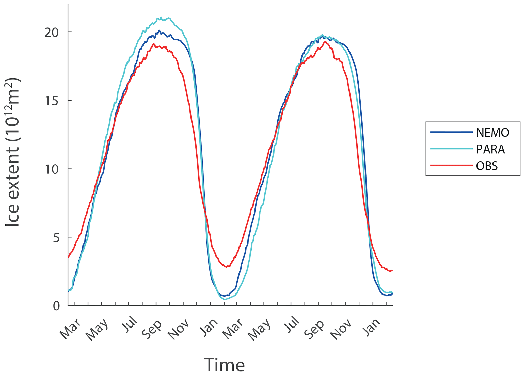
Figure 1Seasonal cycle of the Antarctic sea ice extent (in 1012 m2) in observations (Fetterer et al., 2017) and in the reference experiments with NEMO and PARASO (starting in March). For observations and PARASO, the period from March 1995 to February 1997 is shown, while for NEMO the forcing corresponds to the “normal period” from May 1990 to April 1991 that is applied twice.
The seasonal cycle of Antarctic sea ice extent is highly asymmetric, with a minimum around Julian day 50 (19 February) and a maximum on average close to day 260 (18 September) (Stammerjohn et al., 2008; Massom et al., 2013; Handcock and Raphael, 2020; Raphael et al., 2020; Roach et al., 2022). The advance season, defined as the time between the minimum and maximum ice extents, is thus about 2 months longer than the retreat season, defined as the time from maximum to minimum.
It has been suggested that this asymmetry is related to the variations in the mean position of the westerly winds that blow over the Southern Ocean associated with the semiannual oscillation (SAO) (Enomoto and Ohmura, 1990; Watkins and Simmonds, 1999; Eayrs et al., 2019). This mode of variability in the Antarctic climate induces a larger divergence of the sea ice pack in spring and thus a rapid melting, while the divergence is weaker in fall, leading to a slower expansion of the pack. A complementary mechanism explaining the rapid seasonal retreat of the sea ice is the positive ice–albedo feedback, in which a decrease in ice concentration yields a larger absorption of solar radiation and enhances the ice melting (Gordon, 1981; Nihashi and Cavalieri, 2006). A possible role of the oceanic heat input has also been proposed (Gordon, 1981). However, the vertical ocean heat transport from the relatively warm ocean below the mixed layer to the surface is higher in fall and winter when the stratification is weak than in spring and summer when it is strong (Gordon, 1981; Martinson, 1990). The seasonality of the vertical oceanic transport alone could thus not explain the asymmetry in the seasonal cycle of the sea ice extent (Eayrs et al., 2019), but it could have an indirect effect, for instance through its effect on the ice thickness (Martinson, 1990; Goosse et al., 2018; Wilson et al., 2019).
Nevertheless, a recent study based on idealized climate models has demonstrated that the asymmetry of the seasonal cycle of the ice extent is due to the seasonal cycle of incoming solar radiation (Roach et al., 2022). The period with relatively high incoming solar radiation in spring and summer induces a rapid melting season and a fast retreat of the sea ice, while a long period with low insolation in fall and winter favors a longer growing season. This relatively direct mechanism is very robust and explains why the asymmetry is observed each year and is reproduced by a wide range of models, from very simple ones to the most complex Earth system models (Eayrs et al., 2019; Roach et al., 2022).
Identifying the seasonal cycle of insolation as the main contributor to the asymmetry of the seasonal cycle of the Antarctic sea ice extent is a major achievement. However, the atmosphere, sea ice and ocean dynamics still play a role and may modulate the magnitude of the asymmetry. Furthermore, the seasonal cycle of the sea ice extent is characterized by many other elements in addition to this asymmetry, such as its amplitude or the timing of the maximum retreat. Factors controlling those characteristics also need to be analyzed to quantify how the seasonal cycle of the Antarctic sea ice influences the dynamics of the climate at high southern latitudes. Models still have large biases in those aspects, and a better understanding is necessary for model improvement (Downes et al., 2015; Eayrs et al., 2019; Roach et al., 2020; Raphael et al., 2020; Schroeter and Sandery, 2022).
Several studies have addressed the role of sea ice processes and atmosphere and ocean feedbacks on Antarctic sea ice extent, focusing on both the mean seasonal cycle and the interannual variability (e.g., Fichefet and Morales Maqueda, 1997; Holland and Kimura, 2016; Hobbs et al., 2016; Kusahara et al., 2019). An instructive diagnostic is to decompose the contribution of the dynamics, including the transport of sea ice, from the one of thermodynamics that influences the local formation or melting of sea ice. This decomposition is not always straightforward, as for example winds control both the sea ice transport and the advection of warm or cold air masses that impacts thermodynamics processes. The results may also depend on the definition of the dynamics and thermodynamics contributions. Nevertheless, a common conclusion is that the thermodynamics processes play a strong role nearly all year long, with a clearly dominant contribution during the advance period, while the impact of the winds becomes more important later in the season, in particular during the retreat (Fichefet and Morales Maqueda, 1997; Holland and Kimura, 2016; Kusahara et al., 2019; Eayrs et al., 2020).
Despite those advances, many uncertainties remain around the processes controlling the seasonal cycle of the Antarctic sea ice, in particular because the majority of existing studies address only some of the processes, preventing a comparison between different factors, or are devoted to the variability and trends and not to the seasonal cycle itself. As a consequence, our goal here is to propose an analysis of the different processes in a single framework, using sensitivity experiments designed to study the seasonal cycle. Specifically, we perform sensitivity experiments with a sea ice–ocean model driven by an atmospheric reanalysis and the same model coupled to a regional atmospheric model, disabling or strongly perturbing key processes related to sea ice dynamics and thermodynamics as well as the exchanges between the atmosphere and ocean.
The goal of those sensitivity experiments is not to impose realistic changes or to improve agreement with observations but rather to determine the role of the associated processes. In contrast to many existing sensitivity studies performed with sea ice–ocean models, the experiments with the coupled model will address the limitations associated with a prescribed atmospheric state, which tends to damp the changes imposed by the perturbation as the location of the sea ice edge is strongly controlled by the atmospheric forcing, in particular in winter (e.g., Urrego-Blanco et al., 2016). Furthermore, the comparison between the experiments with and without coupling with the atmosphere will, for the first time, quantify the regional atmospheric feedbacks in response to the imposed perturbation. The sensitivity experiments last only 2 years and are not analyzed at equilibrium for two reasons. First, the drift of the model state after several years in response to the perturbation can be large. The relative importance of the various processes, which may depend of the mean state, can thus be very different from the one in the current climate. Second, by comparing the first year of each experiment, each of which starts with identical conditions at the beginning of the season, and the second year, for which the perturbation has already acted during 1 year, we can determine the contribution of the initial state and the one of the processes occurring during the sea ice advance and retreat seasons. This approach is also instructive for understanding observed changes and for predictions as this distinction between initial conditions and ongoing perturbations is key in interpreting the observed variability. Many studies have demonstrated that large spatial variations are present between the different sectors of the Southern Ocean (e.g., Parkinson et al., 2019; Kusahara et al., 2019; Kacimi and Kwok, 2020). Analyzing them is necessary to have a full picture of the dynamics of the system. Nevertheless, we will focus here first on the ice extent integrated over the whole Southern Ocean, keeping the regional changes for future work except when critically needed to interpret the integrated changes. The models used and the perturbation applied are described in Sect. 2. Section 3 presents the main results of the sensitivity experiments. Section 4 is devoted to the atmospheric feedbacks. Section 5 includes a discussion and a synthesis of our main results.
2.1 Model description
The simulations are performed with a regional circum-Antarctic configuration of the sea ice–ocean model NEMO-LIM3 (Nucleus for European Modelling of the Ocean–Louvain-la-Neuve sea ice model version 3) version 3.6 (Rousset et al., 2015) driven by the ERA5 atmospheric reanalysis (Hersbach et al., 2020) and with NEMO-LIM3 coupled to the COSMO-CLM2 regional atmospheric model (Pelletier et al., 2022a). The model setup and forcing are identical to in Verfaillie et al. (2022) for NEMO-LIM3 driven by ERA5 and to in Pelletier et al. (2022a) for NEMO-LIM–COSMO-CLM2, except that, for the latter, a bug in the interpolation of the winds in the coupling between the ocean and atmosphere has been corrected (Pelletier et al., 2022b). The version of NEMO-LIM3 driven by ERA5 will hereafter be referred to as NEMO and the version coupled to COSMO-CLM2 as PARASO following Pelletier et al. (2022a).
NEMO (Madec et al., 2017) includes the OPA ocean model (Océan PArallélisé) coupled with the Louvain-la-Neuve sea ice model (Vancoppenolle et al., 2012; Rousset et al., 2015). Our configuration has an explicit representation of Antarctic ice shelf cavities using the implementation of Mathiot et al. (2017). The free-surface oceanic component is hydrostatic and applies finite differences to solve the equations on an Arakawa C grid. Vertical mixing is computed using a turbulent kinetic energy (TKE) scheme (Gaspar et al., 1990), while lateral diffusion of momentum is carried out with a bi-Laplacian viscosity and isopycnal diffusion of tracers with a Laplacian operator. Oceanic convection is represented using an enhanced vertical diffusivity, triggered under unstable vertical stratification (Lazar et al., 1999). The sea ice component uses an elastic–viscous–plastic rheology (Bouillon et al., 2013) and a five-category ice thickness distribution (Bitz et al., 2001; Massonnet et al., 2019). Each of those categories is covered by snow, with one snow thickness per category. The energy-conserving sea ice thermodynamics follows Bitz and Lipscomb (1999) and includes an explicit representation of the evolution of salt content and its impact on the sea ice properties (Vancoppenolle et al., 2009). The albedo of sea ice depends on snow and ice thickness, surface temperature, and cloud cover (Grenfell and Perovich, 2004; Brandt et al., 2005).
The model grid is ePERIANT025 (Mathiot et al., 2017), which has a nominal horizonal resolution of with an isotropic spacing, meaning that the resolution is about 24 km at 30∘ S but increases up to 3.8 km over the Antarctic continental shelf. A z coordinate is applied on the vertical using 75 levels, with a thickness of about 1 m at the surface reaching 200 m at depth and partial steps in the bottom layer (and in the top layer beneath ice shelves). In the uncoupled simulations, NEMO is driven at the surface by the fluxes computed by the CORE bulk formulas (Large and Yeager, 2004) using 3-hourly fields derived from the ERA5 reanalysis (Hersbach et al., 2020). The conditions at the northern boundary of the domain (30∘ S) are prescribed from Ocean Reanalysis System 5 (ORAS5; Zuo et al., 2019).
In PARASO, NEMO is coupled to COSMO-CLM2, which includes version 5.0 of the Consortium for Small-scale Modeling (COSMO) regional atmospheric model (Rockel et al., 2008) and the Community Land Model (CLM) version 4.5 (Oleson et al., 2013). COSMO is a non-hydrostatic model using generalized terrain-following height coordinates with 60 levels (Doms et al., 2018). The version utilized here includes parameter calibration adapted to polar regions and a new snow scheme (Souverijns et al., 2018). Furthermore, the computation of the fluxes is separated over land, ocean and sea ice surfaces for the coupling with NEMO (Pelletier et al., 2022a). The conditions at the lateral boundary of the domain are obtained from ERA5. COSMO-CLM2 uses a rotated latitude–longitude grid with a horizontal resolution of 0.22∘, which corresponds to about 25 km. The domain is smaller than the one of NEMO, with a northern boundary located between 50 and 40∘ S. In the areas not simulated by COSMO-CLM2, NEMO is forced by ERA5 fields as in the uncoupled configuration.
2.2 Experimental design
NEMO is driven by the ERA5 reanalysis using, every year, the forcing from the period 1 May 1990 to 30 April 1991, which is considered a normal period regarding the major modes of climate variability (Stewart et al., 2020; Verfaillie et al., 2022). The forcing thus has no interannual variability in order to focus specifically on the seasonal cycle while keeping conditions close to the model climatology. The 2-year simulations analyzed here follow a 10-year spin-up, which is sufficient to have a quasi-equilibrium for the surface variables (Verfaillie et al., 2022). The PARASO simulation initialization year has been set to 1985, and we discuss here 2-year simulations following a 10-year spin-up, meaning that the analyses start in 1995. The conditions are thus slightly different in the two configurations. Nevertheless, the mean states of the coupled and uncoupled models are also different, preventing a direct comparison between them anyway (Fig. 1). Both configurations underestimate the sea ice extent in summer and tend to overestimate it in winter. They also have a delayed and too rapid retreat season. Those biases are similar to those found in many other coupled and uncoupled models (Downes et al., 2015; Eayrs et al., 2019; Roach et al., 2020; Raphael et al., 2020; Schroeter and Sandery, 2022). Each sensitivity experiment will be compared to the reference simulation using the same model configuration and initial state. This standard method implicitly assumes that the biases remain nearly constant in those pairs of experiments, and the effect of those biases on the quantification of the response to the perturbation is largely removed by performing the difference between the experiment results. However, even with this procedure, the biases can still have in some cases a clear impact on the quantification of feedbacks, as discussed in Sect. 4 for the summer sea ice extent. Additionally, in NEMO alone, the model internal variability is very low for the surface variables analyzed in the present study because of the strong constraint provided by the atmospheric forcing. Due to the inclusion of an interactive atmosphere, PARASO can develop some internal variability within its domain despite the fixed condition imposed at the boundaries. Ideally, an ensemble of simulations should be performed for each of the coupled experiments, but this exceeds available computing capacities. Tests with identical configurations but slight perturbations of the initial state indicate that the difference in ice extent due to this internal variability in the model is usually much smaller than 0.2×10⁶ km2, i.e., less than the response to the perturbation in the majority of the experiments, but the possibility that some of the differences between the experiments are just occurring by chance must be kept in mind.
2.3 Setup of the sensitivity experiments
Identical perturbations are applied in NEMO and PARASO on 1 March and 1 September in the 2-year sensitivity experiments (see Table 1). The first two experiments are devoted to the role of the exchanges between sea ice and the oceanic mixed layer. In the first one (Mix100), the ocean temperatures and salinities are homogenized from the surface to 100 m depth at each time step by completely mixing the corresponding grid boxes in each column. This depth roughly corresponds to the seasonal maximum depth of the mixed layer in the model in most ice-covered regions except over the continental shelf (e.g., Barthélemy et al., 2015). The effect of this mixing-scheme perturbation is that the seasonal summer shoaling of the mixed layer due to freshening is removed. The goal is to determine whether such deep summer mixing favors heat storage at the surface and delays the sea ice advance. In the second experiment (NoMassFlux), sea ice growth and melt are no longer associated with freshwater uptake and release. In practice, we thus set all the mass fluxes at the sea ice–ocean interface to zero in NoMassFlux, but this is equivalent to assuming that sea ice salinity is the same as the ocean surface salinity. Therefore, the surface ocean salinity no longer responds to sea ice formation and melting. This modification disables the negative ice production–entrainment feedback (Martinson, 1990) in which the upper-ocean salinity increase due to ice formation induces a mixed-layer deepening and entrainment of deeper warmer water towards the surface that reduces ice formation. The absence of this negative feedback in NoMassFlux could thus potentially accelerate the sea ice advance.
Table 1List of experiments. Each experiment is performed for 2 years with NEMO and PARASO and for two starting dates, 1 March and 1 September. For references in the text, NEMO and PARASO experiments have the additional suffixes NEMO and PARA, respectively, while for the two starting dates we use the suffixes Mar and Sep.
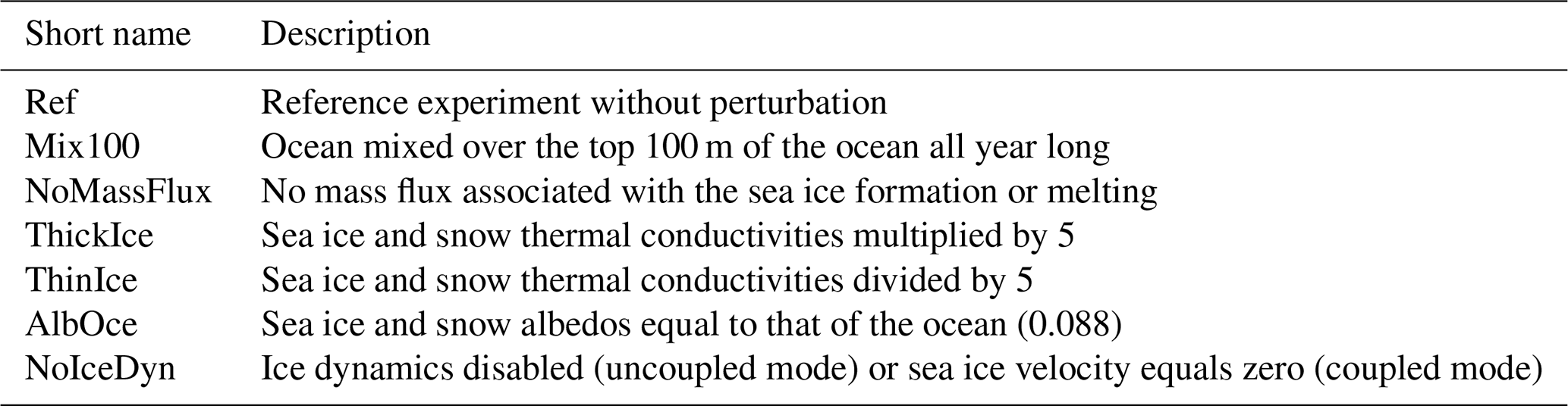
The second group of experiments is devoted to sea ice physics and properties. As sea ice thickness is a key characteristic of the pack that strongly controls its behavior, the first two experiments artificially increase (ThickIce) and decrease (ThinIce) the ice thickness. This is achieved by increasing the thermal conductivities of the ice and snow by a factor of 5 in ThickIce and by decreasing the thermal conductivities of the ice and snow by a factor of 5 in ThinIce. With low conductivity, ice becomes a much better insulator for the ocean that loses less heat to the atmosphere in fall and winter, inducing a slower increase in ice thickness (Maykut, 1986; Bitz and Roe, 2004). From the results of ThickIce and ThinIce, we intend to test the hypothesis that thinner ice will melt faster in spring, accelerating the ice retreat. As the ice–albedo feedback is expected to be a dominant element of the seasonal sea ice retreat (Gordon, 1981; Nihashi and Cavalieri, 2006), setting the albedo of both the snow and the ice to the ocean value in AlbOce should accelerate the retreat.
We also quantify the impact of ice dynamics by disabling it (NoIceDyn). The ice dynamics is expected to favor a faster sea ice advance in fall by transporting sea ice from the colder regions, where it is quickly replaced because of strong ice formation, to the north where it can survive because of the relatively low temperature. It also accelerates the retreat in spring by transferring sea ice to regions where it is warm enough during this season to quickly melt and by creating leads within the pack that enhance the ice–albedo feedback (Fichefet and Morales Maqueda, 1997; Holland and Kimura, 2016; Kusahara et al., 2019; Eayrs et al., 2020). Suppressing ice dynamics should thus reduce the amplitude of the seasonal cycle of the sea ice extent (e.g., Fichefet and Morales Maqueda, 1997). For technical reasons, the implementation of sea ice dynamics suppression differs in uncoupled and coupled experiments: in the former, all the sea ice dynamics components of the model are disabled; in the latter, solely the velocity and large-scale transport are set to zero in PARASO (other mechanisms such as ridging are active).
Although no sensitivity experiment includes explicit modifications of atmospheric parameters or processes, all of the applied perturbations affect indirectly the exchanges between the ocean–sea ice system and the atmosphere by modifying the surface conditions. Comparing the coupled and uncoupled configurations then quantifies the contribution of the atmospheric feedbacks. While the perturbations can potentially influence the atmospheric dynamics and thus winds for instance, we will focus on the feedbacks related to heat exchanges at the surface as they are more directly impacted in the sensitivity experiments.
3.1 First advance season
In the sensitivity experiments starting in March, the perturbations applied to the model physics have very little impact on the sea ice advance until August (Figs. 2a and b and S1 in the Supplement), in both the coupled and the uncoupled model configurations. When starting from identical initial conditions, the sea ice advance seems thus controlled by external conditions imposed by the seasonal evolution of the insolation and does not depend much on the sea ice physics or on the interactions between sea ice, the ocean and the atmosphere. Even the absence of sea ice transport (experiments NoIceDyn_NEMO_Mar and NoIceDyn_PARA_Mar) has a weak effect on the total sea ice extent during this period, confirming previous studies indicating that the sea advance is mainly of a thermodynamic nature (e.g., Fichefet and Morales Maqueda, 1997; Kusahara et al., 2019). The impact on the sea ice volume is more immediate, with a difference that can reach more than a factor of 2 in August between some experiments such as ThickIce_NEMO_Mar and Thin_NEMO_Mar (Fig. 3a). Nevertheless, this change in volume has little impact on the extent, showing a decoupling between the two variables in our experiments during this first advance season.
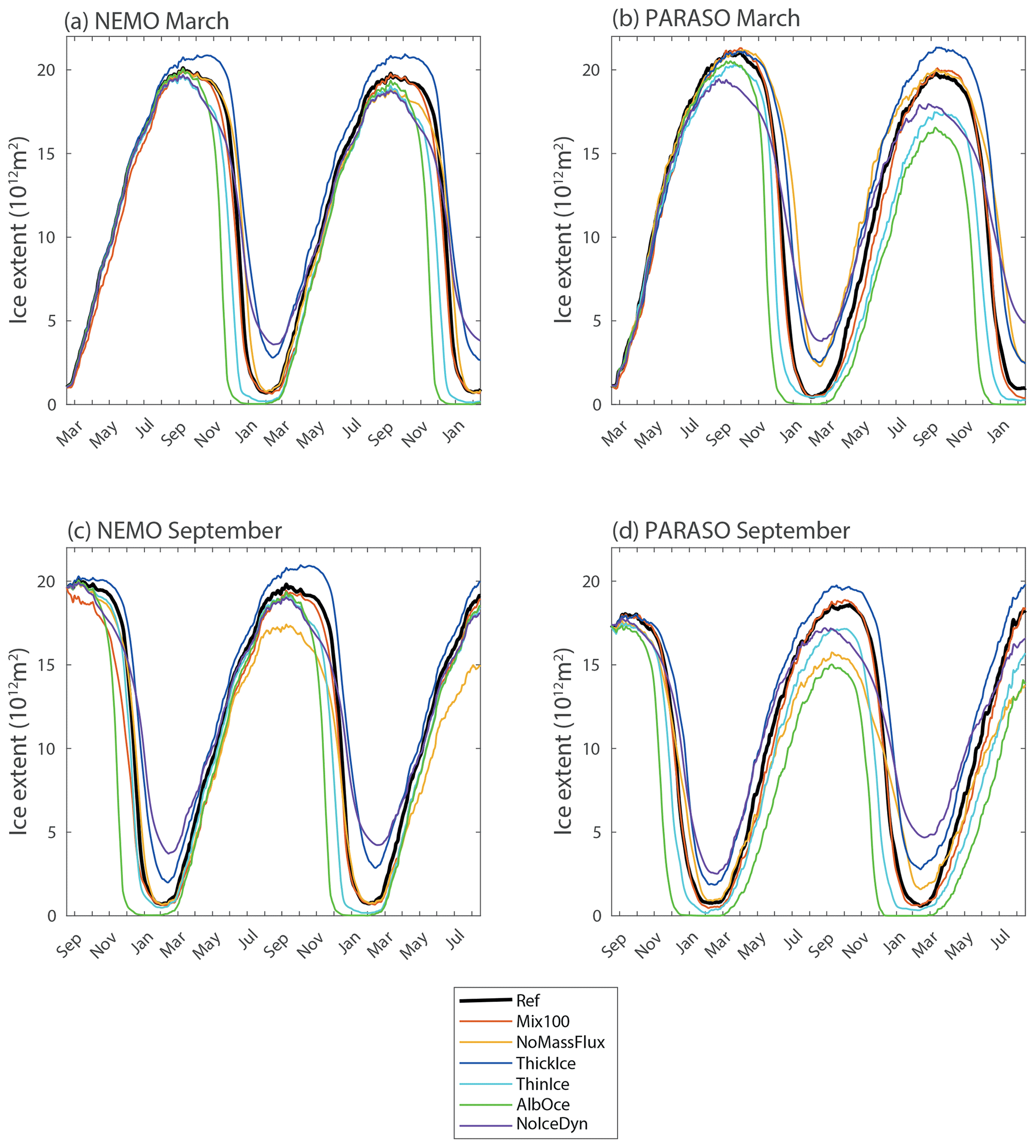
Figure 2Antarctic sea ice extent (in 1012 m2) in the group of experiments starting in March (a, b) and September (c, d) for the NEMO (a, c) and PARASO (b, d) configurations. The equivalent figure showing the anomaly compared to the corresponding reference simulation is provided in Fig. S1.
The different experiments have varying ice growth rates, consistent with the differences in ice volume, but the temporal evolution is relatively similar during the advance season (Figs. 4 and S2). ThickIce and NoMassFlux stand as exceptions. In ThickIce, the ice production–entrainment feedback is very active as a consequence of the large sea ice formation and brine release that destabilizes the water column. The oceanic mixed-layer depth (Fig. S3) is thus much larger than in the other experiments, and the associated vertical ocean-to-ice sensible heat transfer compensates early in the season for a significant fraction of the cooling imposed at the surface, explaining the early peak in the freezing rate (for instance the peak occurs on day 166 in ThickIce_NEMO_Mar compared to day 220 in the corresponding reference simulation). In NoMassFlux, by contrast, as the ice production–entrainment feedback is inactive by design, the oceanic mixing is much weaker and strong ice formation can be sustained until the end of the growth season, particularly in the PARASO configuration, with a peak in ice formation in NoMassFlux_PARA_Mar on day 247 compared to day 187 in the corresponding reference simulation.

Figure 3Antarctic sea ice volume (in 1012 m3) in the group of experiments starting in March (a, b) and September (c, d) for the NEMO (a, c) and PARASO (b, d) configurations.

Figure 4Mass flux due to sea ice growth and melt (counted positive for melting) integrated over the Southern Ocean (in 1011 m3 d−1) in the group of experiments starting in March (a, b) and September (c, d) for the NEMO (a, c) and PARASO (b, d) configurations. This diagnostic is evaluated online in NEMO from the different contributions to ice formation and melting but is equivalent to the time derivative of the ice volume. The equivalent figure showing the anomaly compared to the corresponding reference simulation is provided in Fig. S2.
3.2 Maximum extent and retreat season
The modification of the ice volume imposed by the perturbations has only a weak impact on the sea ice extent until August, as indicated above. However, the experiments with thicker ice tend to have a larger sea ice extent after August, a longer plateau with an extent close to the maximum and a slower retreat. This impact of the ice thickness is well illustrated by the comparison between ThickIce_NEMO_Mar and Thin_NEMO_Mar, which have a difference in ice volume in winter of more than 20×1012 m3. ThickIce_NEMO_Mar has a maximum ice extent that is higher than in Thin_NEMO_Mar by 1.2×10⁶ km2, a timing of the maximum extent delayed by 42 d compared to Thin_NEMO_Mar and an extent that is larger than in Thin_NEMO_Mar by 3.3×10⁶ km2 at the end of November (Figs. 2a and S1). The impact of volume differences on the date of the maximum extent itself is generally weak for most of the other experiments (see Tables 2 and 3), but a link between the maximum volume and the date at which the sea ice extent decreases to 95 % of its maximum is clear in most of them (Fig. 5a).
Table 2Values and timings of the maximum and minimum sea ice extents for the 2 years of the sensitivity experiments starting in March. Extents are given in 1012 m2 and timings in Julian days.
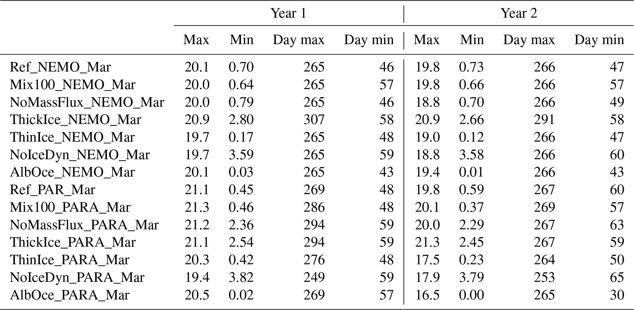
Table 3Values and timings of the maximum and minimum sea ice extents for the 2 years of the sensitivity experiments starting in September. Extents are given in 1012 m2 and timings in Julian days.
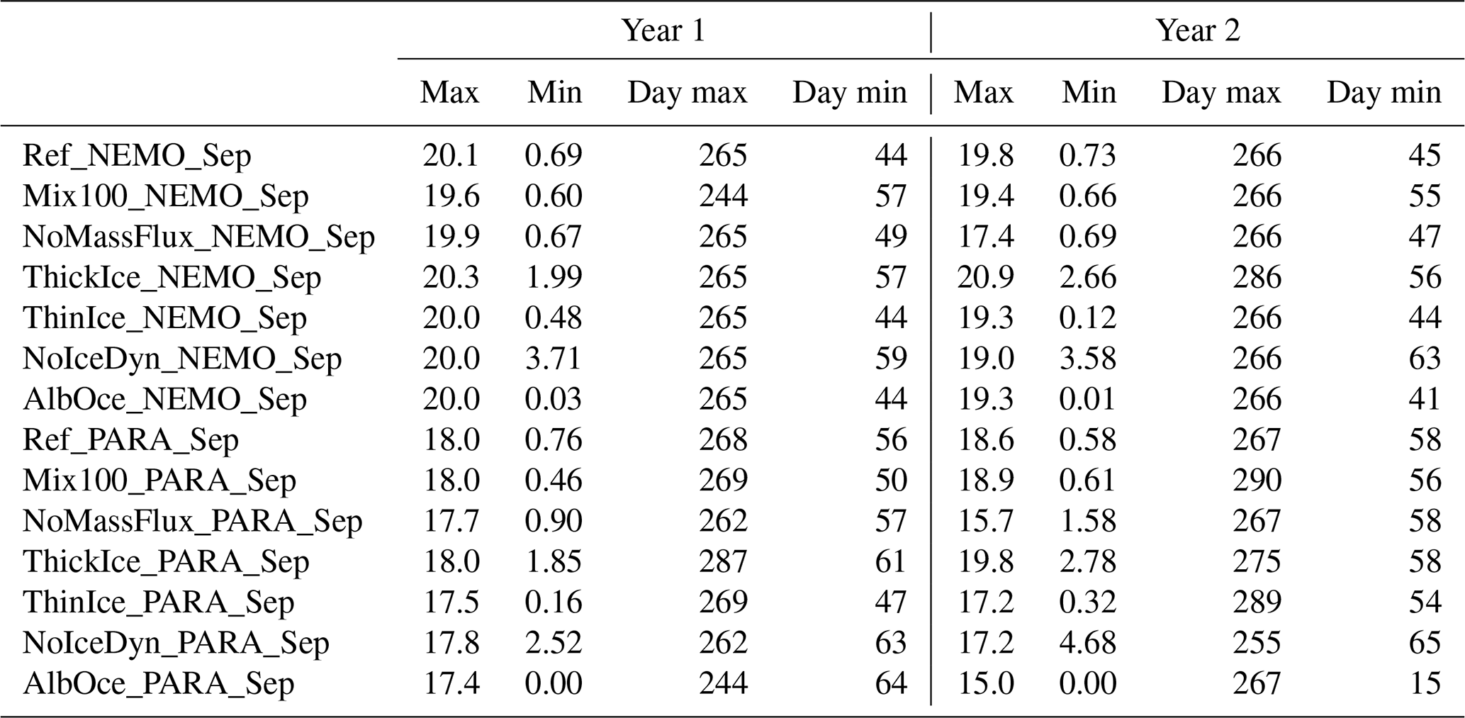

Figure 5(a) Onset of significant seasonal sea ice retreat (day), defined as the number of days after the maximum at which the Antarctic sea ice extent has decreased to 95 % of its maximum value as a function of the maximum ice volume (in 1012 m3). (b) Maximum-sea-ice-extent anomaly (in 1012 m2) compared to the reference experiment as a function of the anomaly in the previous minimum (in 1012 m2) for the second year of the experiments starting in March and for the first minimum and second maximum of the experiments starting in September.
Thicker ice in September tends thus to delay sea ice retreat, as expected. However, the conditions in September (which integrate the effect of the perturbation in model physics, since March in the simulations started at that time) are not the only reason for the difference between the experiments during the retreat season. The experiments starting in September from identical initial conditions tend to diverge nearly immediately, indicating a larger control of sea ice physics on the evolution of the ice extent at this time of the year compared to the advance season (Fig. 2c, d).
This large role for sea ice physics in the melt season is illustrated by the larger differences between the experiments for the timing of the maximum of the ice melting than for the timing of the maximum ice growth rate (Figs. 4 and S2). The maximum ice melting rate spans a range of up to 50 d between the experiments that have the earliest melting (AlbOce) and the latest one (ThickIce, NoMassFlux and NoIceDyn). The faster and earlier melting occurs in AlbOce experiments, as the low albedo in those experiments allows a stronger absorption of incoming solar radiation and thus a larger amount of melt as soon as the Sun is high enough above the horizon. In AlbOce experiments, a large part of the retreat has already been achieved by the end of November. This early and fast retreat leads to a difference in ice extent that can reach more than 10×106 km2 compared to the reference experiments at this time and thus a sea ice extent corresponding to the one simulated only in early January in these reference experiments (Fig. 2). The ThinIce experiments also display an earlier melting than ThickIce ones because of a more efficient ice–albedo feedback, reinforcing the direct effect of the initially thinner ice in winter: it is easier to melt thin sea ice, leading to a higher amount of open water and thus a larger absorption of incoming solar radiation and an intensified melting.
3.3 Minimum extent, subsequent advance season and amplitude of the seasonal cycle
Experiments with earlier melt onset and larger melt rates show faster retreat and lower minimum extent, leading to a larger difference between the experiments in the first summer than in the first winter. In the experiments starting in March, the range of ice extent across all experiments at the first maximum reaches 1.2×10⁶ km2 for NEMO and 1.9×10⁶ km2 for PARASO. For the following minimum in the same experiments, it reaches 3.6×10⁶ and 3.8×10⁶ km2, respectively. The numbers for the summer minimum are relatively similar for the experiments starting in September compared to those starting in March, which suggests that processes in the summer season are more important than the state of the sea ice–ocean–atmosphere system in September (Tables 2 and 3).
By contrast, the state of the sea ice–ocean–atmosphere system in March (i.e., the second year for the experiments starting in March but already the first year for the experiments starting in September) has a dominant influence during the whole sea ice advance season (Marchi et al., 2020). Despite the strong control from the insolation and the limited direct impact of sea ice physics and feedbacks with the ocean and the atmosphere during the first advance season (see above), the model physics thus influences the evolution of the sea ice extent for several months during the second advance season through its effect on the state of the system in March. This is illustrated in Fig. 5b by the association between the positive minimum-sea-ice-extent anomaly and the subsequent positive maximum-extent anomalies present in most experiments, with the notable exception of NoIceDyn experiments as discussed below. In this figure, the minimum sea ice extent is chosen as a proxy for the state of the sea ice and ocean system in summer, but a similar link can be found for other variables, such as the mean summer sea surface temperature southward of 60∘ S (Fig. S4).
The role of the state of the system in March can be illustrated for example using the Mix100 experiments. Increasing the vertical oceanic mixing in the sensitivity experiments redistributes the available energy over the top 100 m without modifying the vertically integrated heat content. This does not have a large influence initially in the experiments starting in March (Fig. 2a). However, the second year in the experiments starting in March is different from the first year as a deeper mixed layer allows a larger heat uptake in summer. Consequently, the Mix100 experiments tend to have a smaller ice extent than the reference experiments during the second sea ice advance season (Figs. 2a and S1).
More generally, for both the coupled and the uncoupled experiments, the summer extent influences the whole advance season and the maximum extent. However, the difference in sea ice extent between the experiments with NEMO tends to decrease with time because of the restoring imposed by a fixed atmospheric state. For instance, the range in the maximum extent for the second year of the experiments beginning in March reaches 2.1×10⁶ km2, while it was 3.6×10⁶ km2 the previous summer (Fig. 2a). By contrast, the range between experiments increases during the sea ice advance season in the PARASO experiments, reaching 4.8×10⁶ km2 for the maximum extent in winter (25 % more than for the summer minimum). While the majority of the experiments displaying a large winter ice extent also have a larger summer ice extent, inducing relatively modest changes in the amplitude of the seasonal cycle, this is not the case in the NoIceDyn experiments. Those experiments are characterized by a reduced amplitude of the seasonal cycle of the sea ice extent, with a smaller extent in winter and a larger one in summer compared to the reference experiments. At the end of the advance season, the ice edge position is set by the advection of sea ice from the south. Sea ice then melts in regions which are too warm to sustain local production (e.g., Holland and Kimura, 2016; Nie et al., 2022). Neglecting ice transport thus leads to an earlier maximum extent and onset of the retreat (Fig. 2). Later during the retreat season, ice is transported northward where it melts, and this transport also enhances the formation of leads within the ice pack that increases solar absorption. Therefore, ice dynamics plays an important role in accelerating the ice retreat, as shown in earlier studies (Fichefet and Morales Maqueda, 1997; Holland and Kimura, 2016; Kusahara et al., 2019; Eayrs et al., 2020), and neglecting this effect in NoIceDyn induces an increase in the minimum ice extent of several million square kilometers (Tables 2 and 3).
3.4 Sensitivity to the starting date in NoMassFlux
Neglecting brine release during ice formation (experiments NoMassFlux) reduces the heat input from the deeper oceanic layer to the surface and results in a clear increase in ice production and volume in the experiments started in March (Fig. 4), in particular in coupled mode. It only has a limited influence on the sea ice extent during the first winter as, by definition, it can only act after sea ice is already present (Martinson, 1990) (Fig. 2). The effect can only be seen indirectly during the sea ice retreat season (when entrainment no longer plays a clear direct role) and the second year, through the influence of the perturbation on the sea ice volume. In particular, this leads to an increase in sea ice extent in NoMassFlux_PARA_Mar of nearly 2.0×10⁶ km2 compared with the corresponding reference experiment in summer (Figs. 2 and S1).
The NoMassFlux experiments starting in September have a different behavior than the experiments beginning in March. As the model has a very low sea ice volume in March, assuming that sea ice has the same salinity as the ocean does not substantially impact the salt and freshwater balance of the model. In contrast, for the experiments starting in September, because of the much larger initial sea ice volume, the NoMassFlux experiments imply a large artificial salt input in the system. The salt input weakens the upper-ocean stratification, enhances mixing, and triggers open-ocean convection and the formation of open-ocean polynyas (Fig. 6). This brings a large amount of heat to the ocean surface, reducing both the sea ice volume and the winter sea ice extent in NoMassFlux_NEMO_Sep and NoMassFlux_Par_Sep compared with the corresponding reference experiments.
3.5 Timing of the maximum and minimum extents
Overall, as expected based on previous studies, the effect of the perturbations prescribed in our sensitivity experiments on the timing of the minimum and maximum ice extents is relatively modest. The largest signal arises in the sea ice dynamics perturbation, which tends to advance the date of the maximum in the coupled experiments (14 and 12 d for the second maximum in NoIceDyn_PAR_Mar and NoIceDyn_PAR_Sep, respectively) and in the experiment with perturbed heat conduction, as the thicker pack can delay the maximum by up to 25 d (in ThickIce_NEMO_Sep). Open-ocean convection can also bring forward the date of the maximum with a third maximum already achieved on day 230 and day 239 of the second year in NoMassFlux_NEMO_Sep and NoMassFlux_PAR_Sep (36 and 28 d earlier compared to the previous year of the same experiment, respectively). The summer minimum can be advanced by up to 43 d in AlbOce_PAR_ Sep through the albedo decrease and delayed by up to 18 d in the sea-ice-dynamics-deprived experiment NoIceDyn_NEMO_Sep. Note that some values in Tables 2 and 3 should be taken with caution as the evolution of sea ice extent is relatively flat close to the maximum and small differences can produce large shifts in the specific day of the maximum (e.g., in Mix100_PAR_Sep and ThinIce_PAR_Sep).
The results discussed in Sect. 3 have highlighted differences between the NEMO and PARASO experiments, and the role of the coupling with the atmosphere is further quantified here. In NEMO, the surface energy budget has only 1 degree of freedom (the surface temperature). Therefore, the surface readily adjusts to the forcing so that the surface temperature closely follows the air temperature, which can be seen as a form of restoring. In PARASO, the surface energy budget responds to both sea ice and atmospheric processes. Another degree of freedom is now that the atmosphere warms or cools in response to changes in sea ice, which in turn affects non-solar (downward longwave and turbulent) fluxes.
This effect of the changes in the atmosphere is evaluated by computing atmospheric feedback factors in response to the perturbation for each pair of coupled and uncoupled model experiments. Feedbacks can be evaluated in different ways. A methodology that is consistent for a wide range of feedbacks, including the standard radiative ones involved in computation of the so-called climate sensitivity as well as non-radiative feedbacks, is to define the feedback factor γ as (Goosse et al., 2018)
where the total response corresponds to the response of the model to some perturbation imposed in the system when all the feedbacks are active, while the reference response is the response of the model to the same imposed perturbation when one feedback or process to be studied (for instance sea ice dynamics) has been left out. As our specific goal is to study the impact of atmospheric coupling, this leads to
and, for sea ice extent specifically,
where ΔSIEPARA and ΔSIENEMO are the changes between the sensitivity experiments and the reference experiments in the PARASO and NEMO configurations, respectively.
The feedback factor can be related to the feedback gain G (e.g., Goosse et al., 2018), defined here as the ratio between the response in coupled mode and the one in uncoupled mode:
A negative value of γ thus corresponds to a negative feedback (changes in PARASO smaller than in NEMO, feedback gain smaller than 1, and the feedback dampens the response to a perturbation); a value between 0 and 1 corresponds to a positive feedback (changes in PARASO larger than in NEMO, feedback gain larger than 1, and the feedback amplifies the perturbation); a value of 1 implies an infinite gain, and values of γ larger than 1 imply a change in the sign of the response between coupled and uncoupled model experiments (negative feedback gain). In the following, we start by discussing the feedback factors lower than 1 (positive and negative feedbacks and positive feedback gains) that are the easiest to interpret in a linear framework, while non-linearities and values of γ larger than 1 (negative feedback gain) will be discussed in the last paragraphs of the section. We must recall here that we were not able to perform ensembles of simulations for our sensitivity experiments, leading to some uncertainties in the evaluation of the model response to the perturbations and thus in the estimate of the feedback parameters. Consequently, we have not analyzed the feedback factors when the coupled response is smaller than 0.2×10⁶ km2 for sea ice extent or 0.2×10³ km3 for sea ice volume, corresponding to very small changes in the system and large feedback factors (the coupled response appears in the denominator of γ). Consistently, we have focused the analyses on the second year of the experiments, as for the first year the changes in several experiments are too small. Nevertheless, even with those criteria, the small internal model variability still has an influence on the estimate of the feedback parameters, and, in particular, it may also contribute to the non-linearities and values of γ larger than 1 discussed below.
4.1 Atmospheric feedbacks on the maximum ice extent
The feedback factors are always positive for the maximum sea ice extent (Fig. 7a), indicating that the coupling with the atmosphere amplifies the wintertime response to perturbations (for the feedback factors smaller than 1; for the ones larger than 1 see below). This matches well our understanding of the system, where sea ice acts as an insulator between the atmosphere and the ocean. An increase in sea ice extent resulting from a perturbation thus cools the atmosphere, which amplifies the initial change, giving a positive feedback. The same positive feedback mechanism applies in the context of an initial decrease in ice extent, leading to atmospheric warming and additional decrease in extent. For example, in AlbOce_PARA_Mar, the surface air temperature is higher than in the reference experiment all year long. The difference reaches 1.5 K on average over the 2 years of the simulations for the oceanic region south of 60∘ S and more than 2.5 K in the second winter (Figs. 8, S5).
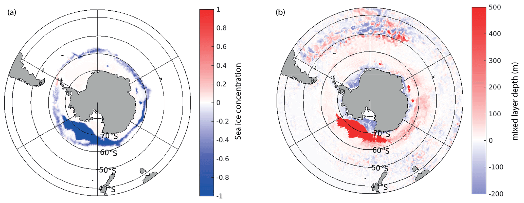
Figure 6Differences in (a) ice concentration and (b) mixed-layer depth (in m) in August of the second year of simulation between NoMassFlux_NEMO_Sep and the corresponding reference experiment.

Figure 7Atmospheric feedback factor for experiments starting in March (blue ×) and September (red +) for (a) the maximum sea ice extent, (b) maximum sea ice volume, (c) minimum sea ice extent and (d) minimum sea ice volume. Light blue lines are drawn at values of 0 and 1 (with positive feedback between those two lines). The equivalent figure for the feedback gain G is given as Fig. S6.
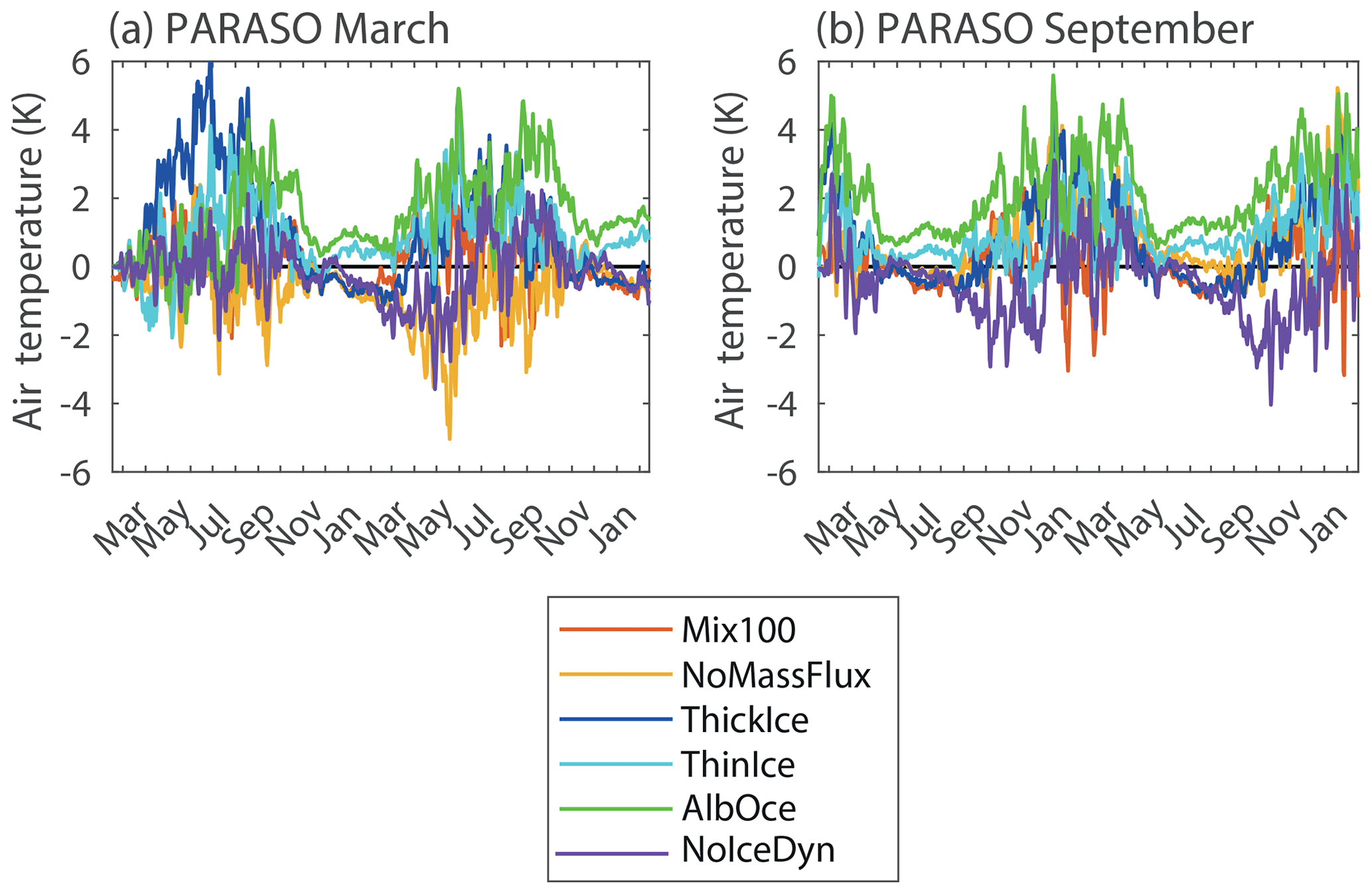
Figure 8Anomaly of surface air temperature (in K) averaged over the oceanic region south of 60∘ S compared to the corresponding reference simulation in the group of experiments starting (a) in March and (b) in September for the PARASO configuration.
Among all the experiments, AlbOce displays the largest feedback gain for the winter ice extent (i.e., γ<1 and closest to 1), with values of γ=0.87 (Fig. 7a) in both experiments started in March and September and hence a feedback gain of 7.7 (Fig. S6a). This is not surprising as the albedo changes associated with sea ice variations are usually considered a key characteristic of polar marine climates. The sea ice–albedo feedback is already active in the NEMO configuration as a change in sea ice concentration affects the surface albedo and thus the net solar radiation absorbed at the surface: in AlbOce_NEMO_Mar and AlbOce_NEMO_Sep, the ocean–sea ice surface south of 60∘ S has a net solar absorption higher than in their reference counterparts of 13 W m−2 in terms of the annual mean (Fig. S7). This is even higher than in AlbOce_PARA_Mar and AlbOce_PARA_Sep, where the change reaches only 7 W m−2. The higher values in the NEMO configuration might be due to differences in the mean state between the coupled and uncoupled model configurations or to feedbacks related to clouds in PARASO, but investigating those effects in more detail is out of the scope of the present study. Nevertheless, the main difference between the coupled and uncoupled experiments comes from the non-solar heat fluxes (Fig. S8), which is the net downward flux associated with incoming and outgoing longwave radiation and latent and sensible heat exchange with the atmosphere. In AlbOce_NEMO_Mar and AlbOce_NEMO_Sep, as the atmospheric state is prescribed, the reduction in sea ice extent and surface warming induce a large increase in non-solar heat losses that reaches 10 and 13 W m−2, respectively, averaged over the area south of 60∘ S. In other words, the artificial restoring to the observed atmospheric state in uncoupled mode makes the non-solar heat loss at the surface nearly compensate for the additional solar heat input. By contrast, the atmospheric warming in AlbOce_PARA_Mar and AlbOce_PARA_Sep only leads to a moderate increase in the non-solar heat losses, with annual mean values of 1 and 4 W m−2, respectively. This explains the larger changes in ice extent in coupled mode (Fig. 2) and the strong drift of the system to a warmer state (Fig. 8).
4.2 Atmospheric feedbacks on maximum ice volume
The feedback factor for the winter volume is also positive in many experiments (Fig. 7b). In particular, the value of γ in NoMassFlux_Mar equals 0.87, corresponding to a feedback gain G of 7.7. In NoMassFlux experiments, the heat input from the ocean to the surface is reduced because of the absence of the ice production–entrainment feedback. This increases ice production and thus ice thickness. In the coupled model integration, the downward non-solar (net longwave and turbulent) fluxes can respond to thicker ice and colder surfaces, which further decreases the surface air temperature by more than 3 K on average over the oceanic region south of 60∘ S during the sea ice growth season. This cooling further enhances the ice production and leads then to a very strong positive atmospheric feedback.
By contrast, the atmosphere provides a negative feedback in the case of the ThinIce and ThickIce experiments. Larger snow and ice thermal conductivities in ThickIce imply larger heat losses from the ocean to the atmosphere in ice-covered regions and thus larger winter sea ice production in all the ThickIce experiments (Fig. 4). In the PARASO configuration, the increased heat conduction from the ice–ocean system warms the lower atmosphere in winter within the ice pack by more than 3 K, integrating over the region south of 60∘ S (Fig. 8). Consequently, the non-solar atmosphere–ice heat fluxes can increase in coupled mode, moderating the increase in sea ice volume compared to the NEMO experiments. In ThinIce, the smaller heat conduction fluxes tend to induce an atmospheric cooling in winter, but this effect is not strong enough to decrease the temperature in the majority of regions, likely because of a dominant effect of the albedo reduction in this experiment. However, cooling is still found close to the continent (Fig. S5). As this is the region where the largest changes in sea ice thickness occur compared to the reference experiment, this dominates the effect of the coupling on the total ice volume. (For more information on the difference between the temperature responses in ThickIce and ThinIce, see the discussion in the Supplement.)
The experimental design in ThickIce and ThinIce may appear counterintuitive as our modifications to the model physics warm the atmosphere when the ice is thicker. Such perturbations highlight a coupling between heat conduction in the ice and non-solar downward atmospheric heat fluxes. When the full system is considered in the real world, we rather experience the effects of the strong coupling between thickness and heat conduction, often referred to as the ice growth–thickness feedback in which an anomalously thin sea ice cover will lose more energy by conduction in winter, leading to thicker and colder ice, reducing the initial anomaly (Maykut, 1986; Bitz and Roe, 2004; Goosse et al., 2018).
4.3 Atmospheric feedbacks on minimum ice extent and volume
Positive feedback factors associated with the coupling with the atmosphere would also be expected for the minimum ice extent (Fig. 7c), in particular because of the amplifying role of the ice–albedo feedback and its impact on air temperature. This interpretation is consistent with the highest summer air temperature in the two experiments with the lowest summer ice extent (ThinIce and AlbOce, Fig. 8). Accordingly, positive values are found in several experiments. However, negative values are also obtained for others. Those positive values may be surprising in particular for AlbOce, but this can be considered an artifact related to the methodology used to compute γ. All the sea ice melts in summer in the AlbOce experiments (Figs. 2 and 3). The response is thus equal to the summer sea ice extent (or volume) in the corresponding reference experiments. As this reference extent (and volume) is slightly higher in the NEMO configuration than in PARASO (Figs. 1 and 2), the response is larger in NEMO, leading to a negative value of γ by definition (Eq. 3).
For ThinIce and ThickIce experiments, the negative atmospheric feedback factors obtained for the summer ice volume (Fig. 7d) are a direct consequence of the negative values discussed above for winter ice volume in the same experiments, with the winter sea ice thickness anomalies persisting until the summer. As those anomalies are particularly large close to the coast, they affect the melting in those regions and thus the feedback factor for the summer sea ice extent, leading to a negative value in ThinIce and values very close to zero in the ThickIce experiments (Fig. 7c).
4.4 Feedback factors larger than 1: impact of the spatial distribution of the response
The analyses of the feedback factors illustrate the non-linearity of the system, for example when comparing the very different values of γ for an increase or a decrease in the conductivity in ThickIce and ThinIce. Values of γ higher than 1 also suggest more complex dynamics than a simple amplification or damping of the response by interactions with the atmosphere as even the sign of the response is different between coupled and uncoupled model configurations. In many cases, this different sign of the response integrated over the whole Southern Ocean, as measured on the anomaly of total sea ice extent or ice volume, is due to a spatially heterogenous response in uncoupled mode. The coupling amplifies or damps the response locally as described by the feedback framework. However, this may change the balance between positive and negative contributions and thus modify the sign of the response integrated over the whole Southern Ocean compared to the uncoupled mode, explaining the value of γ higher than 1.
We will not discuss here all the experiments displaying a value of γ higher than 1, especially because in some cases the difference in the response to the coupling is small and thus probably not very meaningful. Nevertheless, two examples seem illustrative and are detailed below. In NoIceDyn, the sea ice thickness increases in winter close to the coast and decreases close to the ice edge compared to the reference experiment, in both coupled and uncoupled mode (Fig. S9). The integrated volume response is thus a balance between the changes in the two regions, and, depending on their relative strength, the sign of the change in ice volume can change. In coupled mode, the very large increase in thickness close to the coast associated with strong local positive feedbacks with the atmosphere dominates, while in the uncoupled mode, the offshore decrease dominates, then leading to γ greater than 1 for winter ice volume.
At the time of the winter maximum in sea ice extent, sea ice is transported to the ice edge where it tends to melt. The associated freshwater release increases the upper-ocean stratification in the reference experiment, reducing the oceanic heat input to the surface and thus favoring the advance of the pack. (This positive feedback at the ice edge at the time of the maximum ice extent can be contrasted with the negative ice production–entrainment feedback within the pack.) In NoMassFlux_NEMO_Mar, the absence of freshwater release during ice melt leads to a weaker upper-ocean stratification close to the ice edge, allowing deeper mixed layers, with a difference that can reach more than 100 m. As a consequence, the heat input from the ocean to the ice is higher. This is sufficient to limit the seasonal sea ice advance, and the maximum ice extent is lower in NoMassFlux_NEMO_Mar than in the reference experiment by about 1×10⁶ km2 in the second year of the experiments (Fig. 2a). By contrast, the large increase in ice thickness and volume in NoMassFlux_PARA_Mar discussed previously dominates the response even at the ice edge, leading to a positive anomaly in the maximum ice extent. As a consequence, the atmospheric feedback factor is greater than 1. This effect is only seen in the experiments starting in March, as those starting in September are dominated by the consequences of deep mixing and polynya formation within the pack.
We have performed a series of 24 sensitivity experiments to analyze the role of sea ice processes and coupling mechanisms between sea ice, ocean and atmosphere in driving the seasonal cycle of the Antarctic sea ice extent. In order to obtain clear signals and identify the mechanisms at play, deliberately strong and idealized perturbations have been used in our simulations. One limiting aspect arising from making such a design choice is the resulting lack of ability to directly compare the experiments with observational datasets. Furthermore, our quantitative results may be model-dependent, as they can be influenced by the way physical processes are represented in the models and by the biases in the model mean state, which can have a strong influence on the response of models to perturbations (e.g., Goosse et al., 2018; Massonnet et al., 2018). Additionally, the experimental design itself may have an impact on the way some of the processes are evaluated. However, we consider that the relative importance of the different processes and their description are robust, and we will thus focus on those aspects here.
Recall that all the simulations used the same atmospheric forcing (for NEMO simulations) or the same conditions at the boundaries of the domain of the regional atmospheric model that significantly constrain the seasonal evolution of the sea ice (PARASO simulations). Changes in the large-scale atmospheric conditions or in the passage of synoptic storms close to the ice edge are known to have a strong impact on the evolution of the ice extent (e.g., Handcock and Raphael, 2020). While this role of the atmospheric variability is not addressed here, the analyses of the processes at play could provide insight for understanding how the ice–ocean system responds to interannual variations in the atmospheric conditions. In particular, our results are consistent with the large role attributed to the sea ice dynamics and thus to the interannual variability in winds in driving sea ice extent anomalies during the retreat season (e.g., Holland, 2014; Kusahara et al., 2019; Eayrs et al., 2020) as well as with the impact of changes in spring on the sea ice extent trends observed in fall (Holland, 2014). Conversely, the magnitude and relative importance of the different processes and feedbacks investigated in this study may vary from one year to another, as a function of the state of the system or of the large-scale forcing (e.g., Goosse et al., 2018). It would thus be instructive to repeat the analyses performed here for various years and conditions to determine how this affects the value of the feedback parameters.
Our experiments are too idealized to provide explicit recommendations for model improvements, but the identification of the key processes can help to target the changes that might have the largest impact. In particular, the delayed onset of the seasonal sea ice retreat after the maximum present in our simulations can possibly be related to a too thick ice cover close to the winter ice edge, which may be associated with a misrepresentation of processes in the marginal ice zone (Roach et al., 2018, 2019; Alberello et al., 2020; Horvat, 2021). Additionally, the too fast ice retreat in our control runs is likely impacted by the model biases in the sea ice transport because of the dominant role of this process during spring (Holland and Kwok, 2012; Lecomte et al., 2016; Kusahara et al., 2019; Eayrs et al., 2020; Sun and Eisenman, 2021).
We have focused on the sea ice extent integrated over the whole Southern Ocean, although the net influence of a process may be the result of opposite effects between sectors of the Southern Ocean or between coastal regions and the open ocean. For instance, removing ice dynamics tends to increase the ice thickness close to the coast and decrease it at the sea ice edge because of a reduced ice transport, with a clear impact on the temperature changes. This is an illustration that our conclusions derived for the whole ice pack are not necessarily valid for a specific region.
Overall, our results confirm the earlier finding that the model physics has only a moderate effect on the timings of the maximum and minimum Antarctic sea ice extents, which are controlled rather by the insolation cycle (Roach et al., 2022). Deactivating the sea ice dynamics in our models induces an earlier maximum and a tendency towards a later minimum, but the shift is at maximum of the order of 1 week or 2 weeks, which is within the range of year-to-year fluctuations in the observed record. Thicker ice can delay the maximum and a lower albedo lead to an earlier minimum, but similarly this does not strongly modify the shape of the seasonal cycle, in particular its asymmetry. Our experiments are only 2 years in length, and there is a possibility that the shifts would become larger at equilibrium, but in the experiments featuring a clear drift (such as NoIceDyn_PAR and AlbOce_PAR), we observe a change in the values of the maximum and minimum ice extents from the first to the second year rather than in their timing. The only exception is related to strong open-ocean convection that can stop the ice advance season efficiently when it is triggered in the model.
Nevertheless, our results demonstrate that sea ice physics and interactions with the atmosphere and ocean control many other aspects of the seasonal cycle of the ice extent, such as the values of the maximum and minimum and the speed of the retreat. They thus strongly modulate the overall impact of the sea ice in the climate system, in particular on the radiative balance through the modification of the surface albedo and on the exchanges of heat and carbon between the ocean and atmosphere.
Our sensitivity experiments have also illustrated clear distinctions between the dynamics of the sea ice advance and retreat seasons. The sea ice extent advance from March to August is nearly insensitive to the perturbations applied, with nearly identical evolution of the sea ice extent in our experiment over this period if they start from the same initial conditions in March. If the conditions are different in March (e.g., inherited from differences during the previous melting season), this has an effect during the whole advance season. We can interpret those results in the following way. The very weak incoming solar radiation between March and August imposes a large heat loss over the Southern Ocean, and the response of the system depends more on the heat available in March (and thus on conditions at that time) than on any other element in the system. However, the sea ice processes during the ice advance season can have an indirect effect by changing the sea ice thickness and modifying the sea ice extent later in the year. This is the case for the ice production–entrainment feedback that limits the ice growth in winter. During the ice advance season, this has no major impact on the ice extent itself as it modulates the characteristics of sea ice that is already present, but the modification of the thickness has an influence later during the retreat.
The timing of the beginning of the seasonal sea ice retreat and its rate also depend on the late winter conditions, with thicker ice melting later. However, the retreat rate differs strongly between the experiments, and this may have a larger impact on the spring and summer ice extents than the conditions in September. Among all the processes influencing the retreat rate, the ice–albedo feedback is the dominant one, with a lower albedo, whether it is induced directly by a change in albedo (AlbOce) or indirectly by thinner ice (ThinIce) that melts faster, strongly accelerating the ice retreat. The ice transport also plays a clear role by transporting sea ice northward where it melts. Neglecting this process therefore leads to a large increase in summer ice extent. This larger dependence on several key physical processes during the seasonal ice retreat is consistent with the larger climate model sensitivity to changes in parameters in spring and early summer than during the ice advance season (e.g., Urrego-Blanco et al., 2016; Schroeter and Sandery, 2022) and with the larger interannual variability in the melt rates observed over the satellite period than in the growth rates (e.g., Eayrs et al., 2020).
From a prediction point of view, the findings of this paper are also consistent with the idea that the seasonal predictability of Antarctic sea ice extent depends on the season itself (Chevallier et al., 2019; Marchi et al., 2020). A diagnostic predictability study using satellite data has revealed that February is the month for which the sea ice extent anomalies exhibit the largest autocorrelations for all lead times up to 55 d (Chevallier et al., 2019). This higher autocorrelation for February is in line with our findings showing that the seasonal development of sea ice extent during the growing season is controlled minimally by physics but rather by insolation and initial conditions. By contrast, the lowest autocorrelations of sea ice extent anomalies are reached in the melting season, with complete loss of predictability in mid-November. This is again in line with our results that multiple physical factors control the dynamics of sea ice melt.
The impact of all the sea ice and oceanic processes investigated here on the ice extent in winter is amplified by the coupling with the atmosphere, and our experimental design allows us to quantify this amplification. The largest winter atmospheric feedback occurs for perturbations in albedo, as these strongly modify atmospheric temperature and humidity, amplifying the response of the ice. The effect of the ice production–entrainment feedback is also strongly amplified by the atmospheric coupling, as it not only brings thermal energy to the surface that melts ice but also warms up the atmosphere, increasing the response of sea ice. By contrast, negative atmospheric feedbacks can develop for the ice thickness and volume. In particular, larger heat losses due to higher conductive heat fluxes through the sea ice can lead to greater sea ice formation. This induces a larger thermal energy transfer from the ice–ocean system to the atmosphere that reduces the initial heat loss, resulting in a negative atmospheric feedback on the thickness and potentially on the summer extent.
Roach et al. (2022) identified the role of insolation in controlling the observed asymmetry in the growing and melting of Antarctic sea ice. Our idealized sensitivity experiments show that within this robust cycle, the melt rate and maximum and minimum sea ice extents can be affected by sea ice–ocean exchanges, sea ice processes and ice dynamics. We also demonstrated quantitatively how atmospheric feedback can enhance the effect of perturbations but also in some cases dampen it. Although it is an idealized study, it highlights the major role of albedo and sea ice transport in the sea ice extent seasonal cycle and as key processes to target in model development and process understanding.
As described in detail in Pelletier et al. (2022a), the PARASO sources can be obtained by CLM-Community members on their RedC site (https://redc.clm-community.eu/ (last access: 21 January 2022), then “COSMO-CLM”, then “Downloads”). All PARASO sources, except the COSMO routines, are publicly available for didactic purposes at https://doi.org/10.5281/zenodo.5576201 (Pelletier et al., 2021). The files to run the model in the same configuration as here are also available (https://doi.org/10.5281/zenodo.5590053, Pelletier and Helsen, 2021). The NEMO3.6 version is available from https://forge.ipsl.jussieu.fr/nemo/browser/branches/UKMO (Mathiot and Storkey, 2018).
The supplement related to this article is available online at: https://doi.org/10.5194/tc-17-407-2023-supplement.
HG initiated the study and designed the sensitivity experiments after discussions with all the co-authors. FK performed the simulations. FK and PVH prepared the model outputs for the analyses. HG made the analyses and the figures, and all the co-authors contributed in the interpretation of the results. HG wrote the manuscript, with inputs from all co-authors.
The contact author has declared that none of the authors has any competing interests.
Publisher's note: Copernicus Publications remains neutral with regard to jurisdictional claims in published maps and institutional affiliations.
This work was performed in the framework of the PARAMOUR project, “Decadal predictability and variability of polar climate: the role of atmosphere-ocean-cryosphere multiscale interactions”, supported by the Fonds de la Recherche Scientifique – FNRS – and the Research Foundation – Flanders (FWO) under the Excellence of Science (EOS) program (grant no. O0100718F, EOS ID no. 30454083). The computational resources were provided by the VSC (Flemish Supercomputer Center), funded by the FWO and the Government of Flanders; the Center for High Performance Computing and Mass Storage (CISM) of the Université catholique de Louvain (UCL); and the Consortium des Équipements de Calcul Intensif en Fédération Wallonie-Bruxelles (CÉCI), funded by the Fonds de la Recherche Scientifique de Belgique (F.R.S.-FNRS) under convention 2.5020.11 and by the Walloon Region. Hugues Goosse is research director with the F.R.S.-FNRS. Edward Blanchard-Wrigglesworth was supported by the Office of Naval Research DRI grant N00014-18-1-2175. Lettie A. Roach was supported by the National Oceanic and Atmospheric Administration (NOAA) Climate and Global Change Postdoctoral Fellowship Program, which is administered by UCAR's Cooperative Programs for the Advancement of Earth System Science (CPAESS) under award NA18NWS4620043B.
This research has been supported by the Fonds de la Recherche Scientifique – FNRS (grant no. O0100718F, EOS ID no. 30454083), the National Oceanic and Atmospheric Administration (grant no. NA18NWS4620043B) and Office of Naval Research DRI grant N00014-18-1-2175.
This paper was edited by Christian Haas and reviewed by two anonymous referees.
Alberello, A., Bennetts, L., Heil, P., Eayrs, C., Vichi, M., MacHutchon, K., Onorato, M., and Toffoli, A.: Drift of pancake ice floes in the winter antarctic marginal ice zone during polar cyclones, J. Geophys. Res.-Oceans, 125, e2019JC015418, https://doi.org/10.1029/2019JC015418, 2020.
Barthélemy, A., Fichefet, T., Goosse, H., and Madec, G.: Modelling the interplay between sea ice formation and the oceanic mixed layer: limitations of simple brine rejection parameterizations, Ocean Model., 86, 141–152, 2015.
Bitz, C. M. and Lipscomb, W. H.: An energy-conserving thermodynamic model of sea ice, J. Geophys. Res.-Oceans, 104, 15669–15677, https://doi.org/10.1029/1999JC900100, 1999.
Bitz, C. M., Holland, M. M., Weaver, A. J., and Eby, M.: Simulating the ice-thickness distribution in a coupled climate model, J. Geophys. Res.-Oceans, 106, 2441–2463, https://doi.org/10.1029/1999JC000113, 2001.
Bitz, C. M. and Roe, G. H.; A mechanism for the high rate of sea ice thinning in the Arctic Ocean, J. Climate, 17, 3623–3632, 2004.
Bouillon, S., Fichefet, T., Legat, V., and Madec, G.: The elastic– viscous–plastic method revisited, Ocean Model., 71, 2–12, https://doi.org/10.1016/j.ocemod.2013.05.013, 2013.
Brandt, R. E., Warren, S. G., Worby, A. P., and Grenfell, T. C.: Surface Albedo of the Antarctic Sea Ice Zone, J. Climate, 18, 3606–3622, https://doi.org/10.1175/JCLI3489.1, 2005.
Chevallier, M., Massonnet, F., Goessling, H., Guémas, V., and Jung, T. : The Role of Sea Ice in Sub-seasonal Predictability, In Sub-Seasonal to Seasonal Prediction, Elsevier, 201–221, https://doi.org/10.1016/B978-0-12-811714-9.00010-3, 2019.
Doms, G., Förstner, J., Heise, E., Herzog, H.-J., Mironov, D., Raschendorfer, M., Renhardt, T., Ritter, B., Schrodin, R., Schulz, J.-P., and Vogel, G.: COSMO-Model Version 5.05: A Description of the Nonhydrostatic Regional COSMO-Model – Part I: Dynamics and Numerics, Tech. rep., Consortium for Small-Scale Modelling, https://doi.org/10.5676/DWD_PUB/NWV/COSMODOC_5.05_II, 2018.
Downes, S. M., Farneti, R., Uotila, P., Griffies, S. M., Marsland, S. J., Bailey, D., Behrens, E., Bentsen, M., Bi, D., Biastoch, A., Böning, C., Bozec, A., Canuto, V. M., Chassignet, E., Danabasoglu, G., Danilov, S., Diansky, N., Drange, H., Fogli, P. G., Gusev, A., Howard, A., Ilicak, M., Jung, T., Kelley, M., Large, W. G., Leboissetier, A., Long, M., Jianhua, L., Masina, S., Mishra, A., Antonio Navarra, A. J., Nurser, G., Patara, L., Samuels, B. L., Sidorenko, D., Spence, P., Tsujino, H., Wang, Q., and Yeager, S. G.: An assessment of southern ocean water masses and sea ice during 1988–2007 in a suite of interannual core-ii simulations, Ocean. Model., 94, 67–94, https://doi.org/10.1016/j.ocemod.2015.07.022, 2015.
Eayrs, C., Holland, D. M., Francis, D., Wagner, T. J. W., Kumar, R., and Li, X.: Understanding the seasonal cycle of Antarctic sea ice extent in the context of longer-term variability, Rev. Geophys., 57, 1037–1064, https://doi.org/10.1029/2018RG000631, 2019.
Eayrs, C., Faller, D., and Holland, D. M.: Mechanisms driving the asymmetric seasonal cycle of Antarctic Sea Ice in the CESM Large Ensemble, Ann. Glaciol., 61, 171–180, https://doi.org/10.1017/aog.2020.26, 2020.
Enomoto, H. and Ohmura, A.: The influences of atmospheric half-yearly cycle on the sea ice extent in the Antarctic, J. Geophys. Res., 95, 9497, https://doi.org/10.1029/JC095iC06p09497, 1990.
Fetterer, F., Knowles, K., Meier, W. N., Savoie, M., and Windnagel, A. K.: Sea Ice Index, Version 3, Boulder, Colorado USA. National Snow and Ice Data Center [data set], https://nsidc.org/data/g02135/versions/3 (last access: 10 October 2021), 2017.
Fichefet, T. and Morales Maqueda, M. A.: Sensitivity of a global sea ice model to the treatment of ice thermodynamics and dynamics, J. Geophys. Res., 102, 12609–12646, 1997.
Gaspar, P., Grégoris, Y., and Lefevre, J.-M.: A simple eddy kinetic energy model for simulations of the oceanic vertical mixing: Tests at station Papa and long-term upper ocean study site, J. Geophys. Res.-Oceans, 95, 16179–16193, https://doi.org/10.1029/JC095iC09p16179, 1990.
Goosse, H., Kay, J. E., Armour, K., Bodas-Salcedo, A., Chepfer, H., Docquier, D., Jonko, A., Kushner, P. J., Lecomte, O., Massonnet, F., Park, H.-S., Pithan, F., Svensson, G., and Vancoppenolle, M.: Quantifying climate feedbacks in polar regions, Nat. Commun., 9, 1919, https://doi.org/10.1038/s41467-018-04173-0, 2018.
Gordon, A. L.: Seasonality of Southern Ocean sea ice, J. Geophys. Res., 86, 4193284, https://doi.org/10.1029/JC086iC05p04193, 1981.
Grenfell, T. C. and Perovich, D. K.: Seasonal and spatial evolution of albedo in a snow-ice-land-ocean environment, J. Geophys. Res.-Oceans, 109, 8044, https://doi.org/10.1029/2003JC001866, 2004.
Handcock, M. S. and Raphael, M. N.: Modeling the annual cycle of daily Antarctic sea ice extent, The Cryosphere, 14, 2159–2172, https://doi.org/10.5194/tc-14-2159-2020, 2020.
Hersbach, H., Bell, B., Berrisford, P., Hirahara, S., Horányi, A., Muñoz-Sabater, J., Nicolas, J., Peubey, C., Radu, R., Schepers, D., Simmons, A., Soci, C., Abdalla, S., Abellan, X., Balsamo, G., Bechtold, P., Biavati, G., Bidlot, J., Bonavita, M., De Chiara, G., Dahlgren, P., Dee, D., Diamantakis, M., Dragani, R., Flemming, J., Forbes, R., Fuentes, M., Geer, A., Haimberger, L., Healy, S., Hogan, R. J., Hólm, E., Janisková, M., Keeley, S., Laloyaux, P., Lopez, P., Lupu, C., Radnoti, G., de Rosnay, P., Rozum, I., Vamborg, F., Villaume, S., and Thépaut, J.-N.: The ERA5 global reanalysis, Q. J. Roy. Meteor. Soc., 146, 1999–2049, https://doi.org/10.1002/qj.3803, 2020.
Hobbs, W. R., Massom, R., Stammerjohn, S., Reid, P., Williams, G., and Meier, W.: A review of recent changes in Southern Ocean sea ice, their drivers and forcings, Global Planet. Change, 143, 228–250, https://doi.org/10.1016/j.gloplacha.2016.06.008, 2016.
Holland, P. R.: The seasonality of Antarctic sea ice trends, Geophys. Res. Lett., 41, 4230–4237, https://doi.org/10.1002/2014GL060172, 2014.
Holland, P. R. and Kimura, N.: Observed Concentration Budgets of Arctic and Antarctic Sea Ice, J. Climate, 29, 5241–6249, 2016.
Holland, P. R. and Kwok, R.: Wind-driven trends in Antarctic sea-ice drift, Nat. Geosci., 5, 872–875, https://doi.org/10.1038/ngeo1627, 2012.
Horvat, C.: Marginal ice zone fraction benchmarks sea ice and climate model skill, Nat. Commun., 12, 2221, https://doi.org/10.1038/s41467-021-22004-7, 2021.
Kacimi, S. and Kwok, R.: The Antarctic sea ice cover from ICESat-2 and CryoSat-2: freeboard, snow depth, and ice thickness, The Cryosphere, 14, 4453–4474, https://doi.org/10.5194/tc-14-4453-2020, 2020.
Kusahara, K., Williams, G., Massom, R., Reid, P., and Hasumi, H.: Spatiotemporal dependence of Antarctic sea ice variability to dynamic and thermodynamic forcing: A coupled ocean–sea ice model study, Clim. Dynam., 52, 3791–3807, https://doi.org/10.1007/s00382-018-4348-3, 2019.
Large, W. G. and Yeager, S. G: Diurnal to decadal global forcing for ocean and sea-ice models: The data sets and flux climatologies, Tech. Rep., National Center for Atmospheric Research [data set], https://doi.org/10.5065/D6KK98Q6, 2004.
Lazar, A., Madec, G., and Delecluse, P.: The deep interior downwelling, the Veronis effect, and mesoscale tracer transport parameterizations in an OGCM, J. Phys. Oceanogr., 29, 2945–2961, https://doi.org/10.1175/1520-0485(1999)029<2945:TDIDTV>2.0.CO;2, 1999.
Lecomte, O., Goosse, H., Fichefet, T., Holland, P. R., Uotila, P., Zunz, V., and Kimura, N.: Impact of surface wind biases on the Antarctic sea ice concentration budget in climate models, Ocean Model., 105, 60–70, https://doi.org/10.1016/j.ocemod.2016.08.001, 2016.
Madec, G., Bourdallé-Badie, R., Bouttier, P.-A., Bricaud, C., Bruciaferri, D., Calvert, D., Chanut, J., Clementi, E., Coward, A., Delrosso, D., Ethé, C., Flavoni, S., Graham, T., Harle, J., Iovino, D., Lea, D., Lévy, C., Lovato, T., Martin, N., Masson, S., Mocavero, S., Paul, J., Rousset, C., Storkey, D., Storto, A., and Vancoppenolle, M.: NEMO ocean engine, Tech. rep., Insitut Pierre-Simon Laplace, Zenodo [code], https://doi.org/10.5281/zenodo.3248739, 2017.
Marchi, S., Fichefet, T., Goosse, H.: influence of the initial ocean state on the predictability of the Antarctic sea ice at the seasonal timescale: a study with NEMO3.6-LIM3, Ocean Model., 148, 101591, https://doi.org/10.1016/j.ocemod.2020.101591, 2020.
Martinson, D. G.: Evolution of the Southern Ocean winter mixed layer and sea ice-open ocean deep-water formation and ventilation, J. Geophys. Res.-Oceans, 95, 11641–11654, 1990.
Massom, R., Reid, P., Stammerjohn, S., Raymond, B., Fraser, A., Ushio, S.: Change and variability in East Antarctic sea ice seasonality, 1979/80–2009/10, PLoS ONE, 8, e64756, https://doi.org/10.1371/journal.pone.0064756, 2013.
Massonnet, F., Vancoppenolle, M., Goosse, H., Docquier, D., Fichefet, T., Blanchard-Wrigglesworth, E., and Bitz, C. M.: Arctic sea-ice variability tied to its mean state through thermodynamic feedbacks, Nat. Clim. Change, 8, 599–603, 10.1038/s41558-018-0204-z, 2018.
Massonnet, F., Barthélemy, A., Worou, K., Fichefet, T., Vancoppenolle, M., Rousset, C., and Moreno-Chamarro, E.: On the discretization of the ice thickness distribution in the NEMO3.6-LIM3 global ocean–sea ice model, Geosci. Model Dev., 12, 3745–3758, https://doi.org/10.5194/gmd-12-3745-2019, 2019.
Mathiot, P. and Storkey, D.: NEMO model code, MetOffice (UK) branch dev_isf_remapping_UKESM_GO6package_r9314, revision 11248, MetOffice [code], https://forge.ipsl.jussieu.fr/nemo/browser/branches/UKMO/dev_isf_remapping_UKESM_GO6package_r9314?rev=15667 (last access: 21 January 2022), 2018.
Mathiot, P., Jenkins, A., Harris, C., and Madec, G.: Explicit representation and parametrised impacts of under ice shelf seas in the z∗ coordinate ocean model NEMO 3.6, Geosci. Model Dev., 10, 2849–2874, https://doi.org/10.5194/gmd-10-2849-2017, 2017.
Maykut, G. A.: The surface heat and mass balance, The Geophysics of Sea Ice, edited by: Untersteiner, N., Plenum Press, 395–464, ISBN 978-1-4899-5354-4, 1986.
Nie, Y., Uotila, P., Cheng, B., Massonnet, F., Kimura, N., Cipollone, A., and Lv, X.: Southern Ocean sea ice concentration budgets of five ocean-sea ice reanalyses, Clim. Dynam., 59, 3265–3285, https://doi.org/10.1007/s00382-022-06260-x, 2022.
Nihashi, S. and Cavalieri, D. J.: Observational evidence of a hemispheric-wide ice–ocean albedo feedback effect on Antarctic sea-ice decay, J. Geophys. Res., 111, C12001, https://doi.org/10.1029/2005JC003447, 2006.
Oleson, K. W., Lawrence, D. M., Bonan, G. B., Drewniak, B., Huang, M., Koven, C. D., Levis, S., Li, F., Riley, W. J., Subin, Z. M., Swenson, S. C., Thornton, P. E., Bozbiyik, A., Fisher, R., Heald, C. L., Kluzek, E., Lamarque, J.-F., Lawrence, P. J., Leung, L. R., Lipscomb, W., Muszala, S., Ricciuto, D. M., Sacks, W., Sun, Y., Tang, J., and Yang, Z.-L.: Technical Description of version 4.5 of the Community Land Model (CLM), Tech. Rep. July, NCAR, http://www.cesm.ucar.edu/models/cesm1.2/clm/CLM45_Tech_Note.pdf (last access: 21 January 2022), 2013.
Parkinson, C. L.: Global Sea Ice Coverage from Satellite Data: Annual Cycle and 35-Yr Trends, J. Climate, 27, 9377–9382, 2014.
Parkinson, C. L.: A 40-y record reveals gradual Antarctic sea ice increases followed by decreases at rates far exceeding the rates seen in the Arctic, Proc. Nat. Acad. Sciences 116, 14414–14423, 10.1073/pnas.1906556116, 2019.
Pelletier, C. and Helsen, S.: PARASO ERA5 forcings, Zenodo [data set], https://doi.org/10.5281/zenodo.5590053, 2021.
Pelletier, C., Klein, F., Zipf, L., Haubner, K., Mathiot, P., Pattyn, F., Moravveji, E., and Vanden Broucke, S.: PARASO source code (no COSMO), Zenodo [code], https://doi.org/10.5281/zenodo.5576201, 2021.
Pelletier, C., Fichefet, T., Goosse, H., Haubner, K., Helsen, S., Huot, P.-V., Kittel, C., Klein, F., Le clec'h, S., van Lipzig, N. P. M., Marchi, S., Massonnet, F., Mathiot, P., Moravveji, E., Moreno-Chamarro, E., Ortega, P., Pattyn, F., Souverijns, N., Van Achter, G., Vanden Broucke, S., Vanhulle, A., Verfaillie, D., and Zipf, L.: PARASO, a circum-Antarctic fully coupled ice-sheet–ocean–sea-ice–atmosphere–land model involving f.ETISh1.7, NEMO3.6, LIM3.6, COSMO5.0 and CLM4.5, Geosci. Model Dev., 15, 553–594, https://doi.org/10.5194/gmd-15-553-2022, 2022a.
Pelletier C., Fichefet, T., Goosse, H., Haubner, K., Helsen, S., Huot, P.-V., Kittel, C., Klein, F., Le clec'h, S., van Lipzig, N. P. M., Marchi, S., Massonnet, F., Mathiot, P., Moravveji, E., Moreno, E., Ortega, P., Pattyn, F., Souverijns, N., Van Achter, G., Vanden Broucke, S., Vanhulle, A., Verfaillie, D., and Zipf, L.: Corrigendum to “PARASO, a circum-Antarctic fully coupled ice-sheet–ocean–sea-ice–atmosphere–land model involving f.ETISh1.7, NEMO3.6, LIM3.6, COSMO5.0 and CLM4.5” published in Geosci. Model Dev., 15, 553–594, 2022, https://doi.org/10.5194/gmd-15-553-2022-corrigendum, 2022b.
Raphael, M. N., Handcock, M. S., Holland, M. M., and Landrum, L. L.: An assessment of the temporal variability in the annual cycle of daily Antarctic sea ice in the NCAR Community Earth System Model, Version 2: A comparison of the historical runs with observations, J. Geophys. Res.-Oceans 125, e2020JC01645, https://doi.org/10.1029/2020JC016459, 2020.
Roach, L. A., Horvat, C., Dean, S. M., and Bitz, C. M.: An emergent sea ice floe size distribution in a global coupled ocean-sea ice model, J. Geophys. Res.-Oceans, 123, 4322–4337, https://doi.org/10.1029/2017JC013692, 2018.
Roach, L. A., Bitz, C. M., Horvat, C., and Dean, S. M.: Advances in modeling interactions between sea ice and ocean surface waves, J. Adv. Model Earth Sy., 11, 4167–4181, https://doi.org/10.1029/2019MS001836, 2019.
Roach, L. A., Dörr, J., Holmes, C. R., Massonnet, F., Blockley, E.W., Notz, D., Rackow, T., Raphael, M. N., O'Farrell, S. P., Bailey, D. A., and Bitz, C. M.: Antarctic sea ice area in CMIP6, Geophys. Res. Lett., 47, e2019GL086729, https://doi.org/10.1029/2019GL086729, 2020.
Roach, L. A., Eisenman, I., Wagner, T. J. W., Blanchard-Wrigglesworth, E., and Bitz, C. M.: Asymmetry in the seasonal cycle of Antarctic sea ice due to Insolation, Nat. Geosci., 15, 277–281, https://doi.org/10.1038/s41561-022-00913-6, 2022.
Rockel, B., Will, A., and Hense, A.: The regional climate model COSMO-CLM (CCLM), Meteorol. Z., 17, 347–348, https://doi.org/10.1127/0941-2948/2008/0309, 2008.
Rousset, C., Vancoppenolle, M., Madec, G., Fichefet, T., Flavoni, S., Barthélemy, A., Benshila, R., Chanut, J., Levy, C., Masson, S., and Vivier, F.: The Louvain-La-Neuve sea ice model LIM3.6: global and regional capabilities, Geosci. Model Dev., 8, 2991–3005, https://doi.org/10.5194/gmd-8-2991-2015, 2015.
Schroeter, S. and Sandery, P. A.: Large-ensemble analysis of Antarctic sea ice model sensitivity to parameter uncertainty, Ocean Model., 177, 102090, https://doi.org/10.1016/j.ocemod.2022.102090, 2022.
Souverijns, N., Gossart, A., Gorodetskaya, I. V., Lhermitte, S., Mangold, A., Laffineur, Q., Delcloo, A., and van Lipzig, N. P. M.: How does the ice sheet surface mass balance relate to snowfall? Insights from a ground-based precipitation radar in East Antarctica, The Cryosphere, 12, 1987–2003, https://doi.org/10.5194/tc-12-1987-2018, 2018.
Stammerjohn, S. E., Martinson, D. G., Smith, R. C., Yuan, X., and Rind, D.: Trends in Antarctic annual sea ice retreat and advance and their relation to El Niño–Southern Oscillation and Southern Annular Mode variability, J. Geophys. Res., 113, 1–20, https://doi.org/10.1029/2007JC004269, 2008.
Stewart, K., Kim, M., Urakawa, S., McC.Hogg, A., Yeager, S., Tsujino, H., Nakano, H., Kiss, A. E., and Danabasoglu, G.: JRA55-do-based repeat year forcing datasets for driving ocean–sea-ice models, Ocean Model., 147, 101557, https://doi.org/10.1016/j.ocemod.2019.101557, 2020.
Sun, S. and Eisenman, I.: Observed Antarctic sea ice expansion reproduced in a climate model after correcting biases in sea icedrift velocity, Nat. Commun., 12, 1060, https://doi.org/10.1038/s41467-021-21412-z, 2021.
Urrego-Blanco, J. R., Urban, N. M., Hunke, E. C., Turner, A. K., and Jeffery, N.: Uncertainty quantification and global sensitivity analysis of the Los Alamos sea ice model, J. Geophys. Res.-Oceans, 121, 2709–2732, https://doi.org/10.1002/2015JC011558, 2016.
Vancoppenolle, M., Fichefet, T., Goosse, H., Bouillon, S., Madec, G., and Maqueda, M. A. M.: Simulating the mass balance and salinity of Arctic and Antarctic sea ice. 1. Model description and validation, Ocean Model., 27, 33–53, https://doi.org/10.1016/j.ocemod.2008.10.005, 2009.
Vancoppenolle, M., Bouillon, S., Fichefet, T., Goosse, H. Lecomte, O., Morales Maqueda, M. A., and Madec, G.: LIM The Louvain-la-Neuve sea Ice Model, Tech. Rep. 31, Note du Pôle de Modélisation de l'Institut Pierre-Simon Laplace No. 31, ISSN No 1288-1619, https://cmc.ipsl.fr/images/publications/scientific_notes/lim3_book.pdf (last access: 21 July 2022), 2012.
Verfaillie, D., Pelletier, C., Goosse, H., Jourdain, N. C., Bull, C. Y. S., Dalaiden, Q., Favier, V., Fichefet, T., and Wille, J.: How does the Southern Annular Mode impact ice-shelf basal melt in Antarctica?, Comm. Earth Env., 3, 139, https://doi.org/10.1038/s43247-022-00458-x, 2022.
Watkins, A. B. and Simmonds, I.: A late spring surge in the open water of the Antarctic sea ice pack, Geophys. Res. Lett., 26, 1481–1484, https://doi.org/10.1029/1999GL900292, 1999.
Wilson, E. A., Riser, S. C., Campbell, E. C., and Wong, A. P.: Winter upper ocean stability and ice-ocean feedbacks in the sea-ice-covered Southern Ocean, J. Phys. Oceanogr., 49, 1099–1117, 2019.
Zuo, H., Balmaseda, M. A., Tietsche, S., Mogensen, K., and Mayer, M.: The ECMWF operational ensemble reanalysis–analysis system for ocean and sea ice: a description of the system and assessment, Ocean Sci., 15, 779–808, https://doi.org/10.5194/os-15-779-2019, 2019.