GLAcier Feature Tracking testkit (GLAFT): a statistically and physically based framework for evaluating glacier velocity products derived from optical satellite image feature tracking

Glacier velocity measurements are essential to understand ice flow mechanics, monitor natural hazards, and make accurate projections of future sea-level rise. Despite these important applications, the method most commonly used to derive glacier velocity maps, feature tracking, relies on empirical parameter choices that rarely account for glacier physics or uncertainty. Here we test two statistics- and physics-based metrics to evaluate velocity maps derived from optical satellite images of Kaskawulsh Glacier, Yukon, Canada, using a range of existing feature-tracking workflows. Based on inter-comparisons with ground truth data, velocity maps with metrics falling within our recommended ranges contain fewer erroneous measurements and more spatially correlated noise than velocity maps with metrics that deviate from those ranges. Thus, these metric ranges are suitable for refining feature-tracking workflows and evaluating the resulting velocity products. We have released an open-source software package for computing and visualizing these metrics, the GLAcier Feature Tracking testkit (GLAFT).

1 Introduction

Accurate measurements of glacier surface velocity are fundamental to answering some of the most societally relevant issues in the cryospheric sciences. Glacier flow speeds underpin many projections of future sea-level rise (Moon et al., 2012; Mouginot et al., 2019; Shepherd et al., 2020), and they are essential for models used to understand the processes that control ice sheet behavior – ice creep, basal sliding, and ice–ocean interactions (Holland et al., 2008; Burgess et al., 2013; Sundal et al., 2013; Zheng, 2022; Van Wyk de Vries et al., 2022). As a sensitive indicator of change, glacier velocities can be used to understand and monitor dangerous glacier surges and detachments (Evans et al., 2009; Shangguan et al., 2021; Van Wyk de Vries et al., 2022) and to quantify freshwater storage volumes in regions reliant on glacier melt as a water resource (Millan et al., 2022; Van Wyk de Vries et al., 2022). In each of these cases, accurate maps of ice velocity with rigorous uncertainty propagation are needed to quantify the total uncertainty envelope of high-impact projections of future change. However, current methods for assessing ice-velocity map quality and uncertainty vary in different workflows and are commonly derived from arbitrary thresholds or measurements over ice-free areas. The workflows and processing software may be easy to use, but the quality assessments for the resulting velocity maps, despite their many applications, rely on researchers who specialize in glacier dynamics. This technical limitation discourages other research and education communities from using glacier velocity data or creates other concerns, such as a risk of over-interpretation during a time-sensitive hazard event.

The most widely used method for deriving glacier velocity at regional or global scales is feature tracking, which is also known as offset tracking, pixel tracking, speckle tracking, template matching, and particle image velocimetry (Bindschadler and Scambos, 1991; Strozzi et al., 2002; Moon et al., 2012; Dehecq et al., 2015; Fahnestock et al., 2016; Friedl et al., 2021). This technique tracks the movement of coherent patterns on the glacier surface (e.g., crevasses, medial moraines, or other optical patterns or radar scatterers) between two satellite image acquisitions. To compute feature displacement, a two-dimensional cross-correlation algorithm is used to prepare a correlation score “surface” for small image chips from the two images. The position of the highest peak in this correlation score surface then corresponds, in an ideal scenario, to the feature displacement between two images. Finally, this process is repeated for each image chip, producing the spatially continuous displacement field which is used to prepare the velocity map with appropriate scaling based on the pixel dimensions and time offset.

Both optical and synthetic aperture radar (SAR) images with a wide range of specifications are suitable for deriving feature-tracked ice velocity, as evidenced by applications using numerous earth-observing satellite datasets (e.g., Armstrong et al., 2016; Strozzi et al., 2017; Van Wychen et al., 2018; Altena et al., 2019; Millan et al., 2019). To date, all of the publicly available ice-velocity datasets with a global extent have been created using feature tracking (Gardner et al., 2019; Friedl et al., 2021; Millan et al., 2022). Despite its popularity, the feature-tracking technique faces challenges involving optimization and ease of use. A feature-tracking workflow contains several adjustable parameters and options, such as image preprocessing methods (typically high-pass or edge filters) and interpolation methods to locate a correlation peak with high precision. Researchers have explored this parameter space, offered recommended settings (Heid and Kääb, 2012; Fahnestock et al., 2016), and released public datasets with extensive documentation such as the NASA ITS_LIVE project (Gardner et al., 2019; Lei et al., 2022). Still, the full parameter space has not been quantitatively studied for a range of different ice flow conditions. Several challenges prohibit further optimization. First, there is no benchmarking test suitable for inter-comparing velocity maps generated with different software packages and parameters. Second, it is challenging to validate the derived velocity maps due to a lack of contemporaneous in situ and satellite observations (Paul et al., 2017).

To lower the threshold of using and assessing feature-tracked glacier velocity maps for various applications, we set out to develop new methods and create a user-friendly, open-source package that can be used to prepare, evaluate, and improve glacier velocity products for a range of science applications. We present the GLAcier Feature Tracking testkit (GLAFT) package, which can easily benchmark the quality of ice-velocity maps using two statistics- and physics-based metrics. The first metric identifies correct feature matches over static ground surfaces and their uncertainty. The second metric analyzes the velocity spatial coherence and evaluates how much the strain rate field reflects the ice flow dynamics.

To demonstrate how the metrics indicate the quality of ice-velocity measurements, we use different parameter settings of various software packages to derive 172 glacier velocity maps for Kaskawulsh Glacier, Canada, from two Landsat 8 and two Sentinel-2 image pairs (Sect. 3.1.1). To evaluate these metrics, the derived velocity maps are compared with simultaneous in situ Global Navigation Satellite System (GNSS) data (Sect. 3.1.2), velocity products from the ITS_LIVE project (Sect. 3.1.3), and a feature-tracking map with an arbitrary synthetic velocity field (Sect. 3.1.4). Finally, we review current approaches for estimating uncertainty and suggest a new framework for quality assessment of derived glacier velocity maps.

2 Defining good performance for glacier feature tracking

To evaluate the success of velocity maps derived from pairs of satellite images, it is necessary to identify the uncertainty of the feature-tracking algorithm used to create them. Since each velocity measurement is derived from the peak location of the cross-correlation surface (in units of pixels along two image axes), the primary source of error depends on the significance of the peak. If the correlation peak has a high signal-to-noise ratio (SNR), we can reasonably assume that the algorithm has found the correct match (i.e., the algorithm identified the same feature in both input images). In this instance, the uncertainty of the resulting pixel offset values (used to derive velocity) is determined by several factors, including the resolution of the input images, uncertainty of image co-registration (Kääb et al., 2016), shape of the correlation peak (Altena et al., 2022), and subpixel resampling errors (Sciacchitano, 2019). Based on simulations, the aggregated inherited uncertainty (2σ) for correct matches falls between 0.02 and 0.4 pixels (Sciacchitano, 2019). On the other hand, if the correlation peak is absent, has a low signal-to-noise ratio, or appears more than once on the correlation surface, the peak-finding algorithm can return an incorrect local maximum, producing an incorrect match and a biased velocity measurement. Since SNR correlates to the matching correctness and provides a good pixel-based quality assessment, many feature-tracking tools generate an SNR map as part of the standard output along with the velocity grid, such as CARST (Zheng et al., 2019, 2021) and GIV (Van Wyk de Vries and Wickert, 2021). Ideally, we want to exclude incorrect matches so that biased measurements do not affect the propagated uncertainty of the derived velocity map. Some published algorithms mask these pixels based on a threshold of SNR (Willis et al., 2012; Dehecq et al., 2015), while others use local coherence (Heid and Kääb, 2012; Lei et al., 2021) or absolute velocity thresholds (Heid and Kääb, 2012) to identify and remove incorrect matches. However, it may be impossible to identify all incorrect matches due to limited a priori knowledge of correct velocity ranges and a lack of ground truth data. Even with a carefully designed mask applied, both correct and incorrect matches are still likely to be present in the velocity map (e.g., Fig. 3 in Heid and Kääb, 2012). As a result, the estimated a posteriori uncertainty (2σ) of the best-filtered feature displacement map is usually about 0.6 to 1.0 pixels (Strozzi et al., 2017; Zheng et al., 2019), 2–3 times larger than the theoretical uncertainty.

In this study we designed global (i.e., image-wide) metrics by considering the arguments above and the computational efficiency, flexibility, and compatibility for existing and emerging workflows that use advanced tracking techniques, such as Altena and Kääb (2020). Along with relevant qualitative assessments (e.g., spatial distribution of incorrect matches), these metrics evaluate how incorrect matches and variation in correct matches alter the true glacier velocity indicated by ice flow physics.

2.1 Metric 1: velocity measurements over static terrain

The first metric is rooted in a traditional approach for calibrating and estimating uncertainty of feature-tracked ice velocity. The central idea is to assume that adjacent ice-free terrain is static without horizontal or vertical movement, implying that any non-zero velocity values in these locations are measurement errors. This approach requires well-distributed control surfaces that cover a large enough area so that the velocity measurements are not heavily influenced by isolated hillslope movements (e.g., Brencher et al., 2021) or landslides (e.g., Shugar et al., 2021; Van Wyk de Vries et al., 2022), which are common in high-mountain environments. The central tendency (mean, median, etc.) of measured velocity components (V_x and V_y, where x and y are defined by the input image axes) over static terrain is traditionally used to calibrate the entire velocity product; see Sect. 3.1.2 for an example. The value of this central tendency can be regarded as the accuracy of the measured feature offset and is controlled by many factors, such as image misalignment, geolocation errors, and atmospheric disturbances (from clouds and ionosphere for optical and SAR images, respectively). In addition to the accuracy-based calibration, the residual variability (standard deviation or other similar metrics) of measured velocity components is conventionally used to assign velocity uncertainty (precision) for the entire product (Heid and Kääb, 2012; Willis et al., 2012; Burgess et al., 2013; Dehecq et al., 2015; Waechter et al., 2015; Paul et al., 2017; Millan et al., 2019). However, this variability is practically an aggregated measurement of correct and incorrect matches and other terrain-dependent errors, and it is challenging to isolate these individual contributions to total observed uncertainty.

Here, we propose a way to better characterize the noise of only the correct matches for the first metric. We use nonparametric, multivariate kernel density estimation (KDE; Silverman, 1986) to differentiate correct and incorrect matches and estimate the variability in the former population. Let V_x,i and V_y,i, $i=\mathrm{1},\mathrm{\dots }N$ be horizontal velocity components from the selected static area containing N measurements (i.e., N pixels). We calculate the kernel density distribution ρ_K at every possible velocity value using the following equation:

$$\begin{array}{}\text{(1)}& {\mathit{\rho }}_K(u,v)={\displaystyle \frac{\mathrm{1}}{Nh}}\sum _{i=\mathrm{1}}^{N}K\left({\displaystyle \frac{u-V_{x,i}}{h}},{\displaystyle \frac{v-V_{y,i}}{h}}\right),\end{array}$$

where (u,v) indicates independent variables along the x and y directions (i.e., two axes in the velocity domain), K is the selected multivariate kernel, and h is the kernel bandwidth. In other words, ρ_K resembles the histogram of the measurements or the sum of individual density distributions centered at $(V_{x,i},V_{y,i})$. Since the choice of kernel does not affect the density estimation as much as bandwidth does, we select the Epanechnikov (parabolic) kernel to achieve computational efficiency due to its finite support compared to the Gaussian kernel. We use the rule-of-thumb method (Silverman, 1986; Henderson and Parmeter, 2012) to determine the bandwidth without prior knowledge about the velocity distribution. Assuming that all the correct matches have an identical, independent, and normally distributed noise term with the same variance in u and v, the rule-of-thumb bandwidth for a multivariate Epanechnikov kernel is calculated as follows:

$$\begin{array}{}\text{(2)}& h=\mathrm{2.1991}\sqrt{{\mathit{\sigma }}_{V_x}{\mathit{\sigma }}_{V_y}}{N}^{-\frac{\mathrm{1}}{\mathrm{6}}},\end{array}$$

where ${\mathit{\sigma }}_{V_x}$ and ${\mathit{\sigma }}_{V_y}$ are the standard deviation of V_x and V_y, respectively. Once a kernel density distribution is found, we locate its main peak value and location on the u–v plane. This peak is assumed to be related to the distribution of the correct matches, and we can design a thresholding method based on peak value to differentiate correct and incorrect matches:

$$\begin{array}{}\text{(3)}& {\mathit{\rho }}_{K_t}={\displaystyle \frac{max\left({\mathit{\rho }}_K\right)}{e^{\frac{z^{\mathrm{2}}}{\mathrm{2}}}}},\end{array}$$

where z is the preselected z score (always positive). Measurements with ${\mathit{\rho }}_K(V_x,V_y)\ge {\mathit{\rho }}_{K_t}$ are considered correct matches, and measurements with ρ_K(V_x,V_y) lower than the same threshold value are classified as incorrect matches. The half ranges of V_x and V_y from correct matches, denoted as δ_u=zσ_u and δ_v=zσ_v, are thus considered zσ uncertainty. In this study, we set z=2 and report 2σ uncertainties for the convenience of comparing previously published results and our results. The variance of the correct matches is also defined as ${\mathit{\sigma }}_u^{\mathrm{2}}=(\frac{{\mathit{\delta }}_u}{z}{)}^{\mathrm{2}}$ and ${\mathit{\sigma }}_v^{\mathrm{2}}=(\frac{{\mathit{\delta }}_v}{z}{)}^{\mathrm{2}}$.

To summarize, while statistics computed over static terrain have previously been used to assess the uncertainty of glacier velocity maps, this study attempts to separate correct and incorrect feature matches over static terrain and to derive uncertainty only from the correct matches. The calculated uncertainty of correct matches can be compared with the theoretical uncertainty (Sciacchitano, 2019). Ideally, the former should approach the latter for optimized measurement precision. In addition, the number of incorrect matches over static terrain and their corresponding velocity distribution can serve as an auxiliary indicator of the accuracy of the velocity map, along with the correct-match uncertainty.

2.2 Metric 2: along-flow strain rates

For computational simplicity, our previous metric overlooks the covariance of the correct matches. However, glacier motion is spatially coherent, and the covariance of neighboring correct matches controls the quality of the measured flow pattern. Hence, the second metric aims to estimate the co-variability in pixels on a glacier using the physics of glacier flow (Cuffey and Paterson, 2010). We start by analyzing the horizontal (two-dimensional) strain rate tensor ${\dot{\mathit{ϵ}}}_{x^{\prime }{x}^{\prime }}$, ${\dot{\mathit{ϵ}}}_{y^{\prime }{y}^{\prime }}$, and ${\dot{\mathit{ϵ}}}_{x^{\prime }{y}^{\prime }}$, where the prime notations of x^′ and y^′ denote along-flow and across-flow directions, respectively. To obtain this tensor, we first calculate the strain rates along the image axes x and y:

$$\begin{array}{}\text{(4)}& \begin{array}{rl}& {\dot{\mathit{ϵ}}}_{xx}={\displaystyle \frac{\partial V_x}{\partial x}},\\ & {\dot{\mathit{ϵ}}}_{yy}={\displaystyle \frac{\partial V_y}{\partial y}},\\ & {\dot{\mathit{ϵ}}}_{xy}={\displaystyle \frac{\mathrm{1}}{\mathrm{2}}}({\displaystyle \frac{\partial V_x}{\partial y}}+{\displaystyle \frac{\partial V_y}{\partial x}}).\end{array}\end{array}$$

In GLAFT, these partial derivatives are computed using 3-by-3 Sobel operators. Next, we compute $\text{arctan2}(V_x/V_y)$ and smooth the results with a two-dimensional median filter with a large window size of 10–35 pixels (depending on the pixel spacing) for the bulk flow direction angle θ (counterclockwise from the x axis). The strain rate tensor is then rotated by θ and projected into the along-flow direction as follows:

$$\begin{array}{}\text{(5)}& \begin{array}{rl}& {\dot{\mathit{ϵ}}}_{x^{\prime }{x}^{\prime }}={\dot{\mathit{ϵ}}}_{xx}{\cos }^{\mathrm{2}}\mathit{\theta }+{\dot{\mathit{ϵ}}}_{yy}{\sin }^{\mathrm{2}}\mathit{\theta }+{\dot{\mathit{ϵ}}}_{xy}\sin \mathrm{2}\mathit{\theta },\\ & {\dot{\mathit{ϵ}}}_{y^{\prime }{y}^{\prime }}={\dot{\mathit{ϵ}}}_{xx}{\sin }^{\mathrm{2}}\mathit{\theta }+{\dot{\mathit{ϵ}}}_{yy}{\cos }^{\mathrm{2}}\mathit{\theta }-{\dot{\mathit{ϵ}}}_{xy}\sin \mathrm{2}\mathit{\theta },\\ & {\dot{\mathit{ϵ}}}_{x^{\prime }{y}^{\prime }}={\displaystyle \frac{\mathrm{1}}{\mathrm{2}}}({\dot{\mathit{ϵ}}}_{yy}-{\dot{\mathit{ϵ}}}_{xx})\sin \mathrm{2}\mathit{\theta }+{\dot{\mathit{ϵ}}}_{xy}\cos \mathrm{2}\mathit{\theta }.\end{array}\end{array}$$

By replacing V_x and V_y with ${\dot{\mathit{ϵ}}}_{x^{\prime }{x}^{\prime }}$ and ${\dot{\mathit{ϵ}}}_{x^{\prime }{y}^{\prime }}$ in Eq. (1), we can calculate the KDE in the strain rate domain and characterize the distribution. We follow the same steps in Eqs. (2)–(3) and find the variance of the strain rate distribution under a preselected z value. To be consistent with the first metric, in this study we report the zσ uncertainty for ${\dot{\mathit{ϵ}}}_{x^{\prime }{x}^{\prime }}$ and ${\dot{\mathit{ϵ}}}_{x^{\prime }{y}^{\prime }}$ as ${\mathit{\delta }}_{x^{\prime }{x}^{\prime }}$ and ${\mathit{\delta }}_{x^{\prime }{y}^{\prime }}$, respectively.

Unlike the case of the previous metric, which indicates the variability from the zero ground truth, the strain rates along a flowing glacier are not zero, but we can still infer a reasonable range based on fundamental physical relationships. Consider a rectangular region on a glacier with one side running across the channel half-width Y and the other side along the flow direction (length X). The average driving stress (${\overline{\mathit{\tau }}}_{\mathrm{d}}$) over the rectangular area is balanced with the basal drag (${\overline{\mathit{\tau }}}_{\mathrm{b}}$), side drag, and longitudinal stress gradient (see Eq. 8.60 of Cuffey and Paterson, 2010, for details):

$$\begin{array}{}\text{(6)}& {\overline{\mathit{\tau }}}_{\mathrm{d}}={\overline{\mathit{\tau }}}_{\mathrm{b}}+{\displaystyle \frac{\mathrm{1}}{Y}}\mathrm{\Delta }\left(H{\overline{\mathit{\tau }}}_{x^{\prime }{y}^{\prime }}\right)+{\displaystyle \frac{\mathrm{1}}{X}}\mathrm{\Delta }\left[H\right(\mathrm{2}{\overline{\mathit{\tau }}}_{x^{\prime }{x}^{\prime }}+{\overline{\mathit{\tau }}}_{y^{\prime }{y}^{\prime }}\left)\right],\end{array}$$

where H is average ice thickness. ${\overline{\mathit{\tau }}}_{x^{\prime }{y}^{\prime }}$, ${\overline{\mathit{\tau }}}_{x^{\prime }{x}^{\prime }}$, and ${\overline{\mathit{\tau }}}_{y^{\prime }{y}^{\prime }}$ represent average shear stress and normal stresses, respectively. Supposing half of the driving stress is balanced by basal drag, and the other half is balanced by side drag, and the longitudinal stress gradient is negligible (cf. Table 8.3 of Cuffey and Paterson, 2010), Eq. (6) becomes

$$\begin{array}{}\text{(7)}& {\overline{\mathit{\tau }}}_{\mathrm{b}}={\displaystyle \frac{\mathrm{1}}{Y}}{\overline{\mathit{\tau }}}_{x^{\prime }{y}^{\prime }}\mathrm{\Delta }H.\end{array}$$

For the right-hand side of Eq. (7), we let ΔH≈H, indicating the maximum possible ice thickness change within the rectangular region. Moreover, we can express the average side drag as a function of the average strain rate, assuming glacier ice can be modeled as a viscous non-Newtonian fluid with the following creep relation (Eq. 3.23 of Cuffey and Paterson, 2010):

$$\begin{array}{}\text{(8)}& {\mathit{\tau }}_{jk}=\mathrm{2}\mathit{\eta }{\dot{\mathit{ϵ}}}_{jk},\end{array}$$

where η is ice viscosity, and the subscripted j and k denote any two of the three dimensions. Thus, Eq. (7) becomes

$$\begin{array}{}\text{(9)}& {\overline{\mathit{\tau }}}_{\mathrm{b}}={\displaystyle \frac{\mathrm{1}}{Y}}\mathrm{2}\mathit{\eta }{\overline{\dot{\mathit{ϵ}}}}_{x^{\prime }{y}^{\prime }}H,\end{array}$$

where ${\overline{\dot{\mathit{ϵ}}}}_{x^{\prime }{y}^{\prime }}$ is the average shear strain rate.

The creep relation (Eq. 8) can also be expressed inversely, known as Glen's flow law:

$$\begin{array}{}\text{(10)}& {\dot{\mathit{ϵ}}}_{jk}=A{\mathit{\tau }}_{jk}^n,\end{array}$$

where n and A are two empirical parameters. Combining Eqs. (8) and (10) leads to the expression of viscosity in terms of the flow-law parameters:

$$\begin{array}{}\text{(11)}& \mathit{\eta }={\displaystyle \frac{\mathrm{1}}{\mathrm{2}A{\mathit{\tau }}_{jk}^{n-\mathrm{1}}}}.\end{array}$$

The along-flow ice speed at the surface ($u_{x^{\prime }}$) can be calculated by integrating Glen's flow law (Eq. 10) along the vertical direction of the ice flow plus the basal slip speed (u_b), assuming a linearly increasing shear stress with depth (see Eqs. 8.32 to 8.35 of Cuffey and Paterson, 2010, for details):

$$\begin{array}{}\text{(12)}& u_{x^{\prime }}=u_{\mathrm{b}}+{\displaystyle \frac{\mathrm{2}A}{n+\mathrm{1}}}{\mathit{\tau }}_{\mathrm{b}}^{n}H.\end{array}$$

Combining Eqs. (11) and (12) with τ_jk set to τ_b leads to the expression of average basal drag as a function of average surface along-flow speed ${\overline{u}}_{x^{\prime }}$ and average basal slip speed ${\overline{u}}_{\mathrm{b}}$:

$$\begin{array}{}\text{(13)}& {\overline{\mathit{\tau }}}_{\mathrm{b}}\approx ({\overline{u}}_{x^{\prime }}-{\overline{u}}_{\mathrm{b}})\mathit{\eta }{\displaystyle \frac{n+\mathrm{1}}{H}}.\end{array}$$

Finally, combining Eqs. (9) and (13) leads to the following equation:

$$\begin{array}{}\text{(14)}& {\displaystyle \frac{{\overline{\dot{\mathit{ϵ}}}}_{x^{\prime }{y}^{\prime }}}{{\overline{u}}_{x^{\prime }}-{\overline{u}}_{\mathrm{b}}}}={\displaystyle \frac{(n+\mathrm{1})Y}{\mathrm{2}{H}^{\mathrm{2}}}},\end{array}$$

which can be further reduced to $\mathrm{2}Y/H^{\mathrm{2}}$ if we assume n=3.

Equation (14) provides a range of plausible ${\dot{\mathit{ϵ}}}_{x^{\prime }{y}^{\prime }}$ values based on glacier speed, channel width, and average ice thickness. Ideally, observed ${\mathit{\delta }}_{x^{\prime }{y}^{\prime }}$ should be as close to ${\overline{\dot{\mathit{ϵ}}}}_{x^{\prime }{y}^{\prime }}$ as possible. If the former is much larger, the glacier velocity likely contains errors, as the observed spatial variability is not physically achievable. On the other hand, if ${\overline{\dot{\mathit{ϵ}}}}_{x^{\prime }{y}^{\prime }}$ is much larger than ${\mathit{\delta }}_{x^{\prime }{y}^{\prime }}$, it is likely that the flow pattern is smoothed too much and has lost real dynamic signals.

3 Tests at Kaskawulsh Glacier

Kaskawulsh Glacier, Yukon, Canada ($\mathrm{60}{}^{\circ }{\mathrm{48}}^{\prime }$ N, $\mathrm{138}{}^{\circ }{\mathrm{36}}^{\prime }$ W; Fig. 1), is an ideal location for demonstrating how these metrics relate to the performance of feature-tracking workflows because it has a nearly continuous GNSS record since 2007, is a wide and long glacier with relatively consistent velocities, and does not surge (Clarke et al., 1986). Kaskawulsh Glacier has an area of 1054 km², stretches ∼ 90 km from the terminus to the farthest ice divide (RGI Consortium, 2017), and has velocities along the main trunk of the glacier ranging from 70 m yr⁻¹ near the terminus to 180 m yr⁻¹ near the confluence of the two main tributaries (Waechter et al., 2015; Gardner et al., 2019). The recent terminus retreat of Kaskawulsh Glacier changed the local hydrology, resulting in a drop in water level at Łù'àn M\”{a}̄n (Kluane Lake), which has impacted indigenous people in the area (Shugar et al., 2017).

Kaskawulsh Glacier has been a research site for decades, with a history of velocity observations dating back to the 1960s. The Icefield Ranges Research Project set up a network of markers to track glacier motion during the 1960s, which concluded there were limited short-term variations in ice velocity (Holdsworth, 1969; Clarke, 2014). More recent work has focused on regional velocity patterns (Burgess et al., 2013; Abe and Furuya, 2015; Waechter et al., 2015; Van Wychen et al., 2018; Altena et al., 2019) and found a multiyear acceleration near Kaskawulsh Glacier's terminus as a terminal lake grew from 2000–2015, followed by a slowdown over the following 5 years after it drained in 2016 (Main et al., 2022).

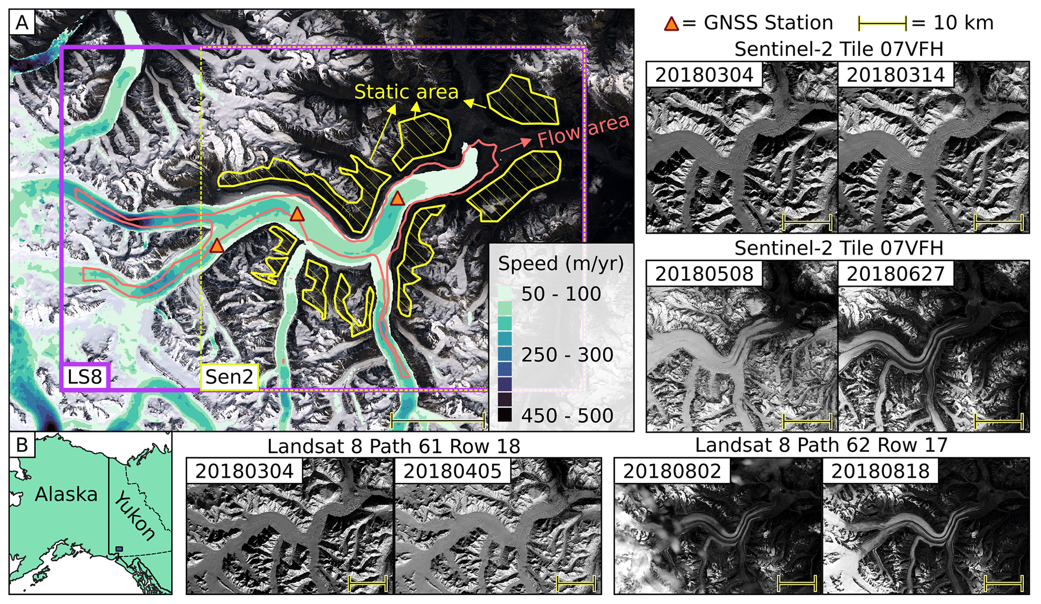
Figure 1 Kaskawulsh Glacier and satellite images used to derive velocity testing maps. (a) Time-averaged glacier velocity (Millan et al., 2022) plotted on a Landsat 8 natural color composite from 9 June 2016. Areas for deriving the proposed metrics are labeled with two types of polygons: static areas in hashed yellow and flow areas in red. Triangles indicate GNSS station positions in 2018. Rectangles show extents of the clipped Landsat 8 (purple) and Sentinel-2 (yellow) images used in this study. (b) Context map for panel (a). Other panels show the clipped images with labels specifying their respective tile numbers and acquisition dates.

3.1 Methods

3.1.1 Deriving glacier velocities

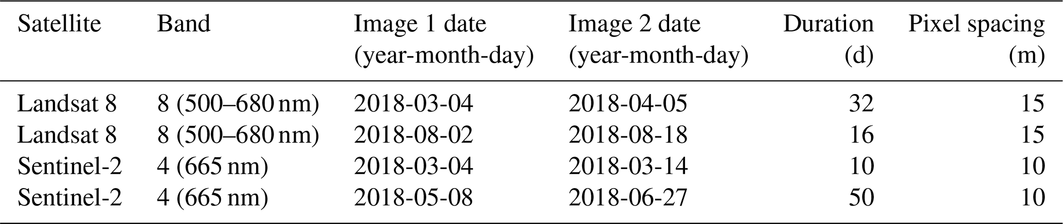
We selected four optical satellite image pairs (Fig. 1, Table 1), each of which has a different time separation and surface conditions. We downloaded the level 2 orthorectified images from the USGS EarthExplorer (https://earthexplorer.usgs.gov/, last access: 21 August 2020) and clipped them to the extent of Kaskawulsh Glacier for processing efficiency. We used four different packages to derive glacier velocity maps, each of which has a distinct method for processing velocity fields, briefly described as follows:

Table 1 Optical images used to derive glacier velocities in this study.

• autoRIFT (autonomous Repeat Image Feature Tracking; Lei et al., 2021) is an open-source feature-tracking toolbox developed at NASA JPL and written in Python and C++; autoRIFT performs normalized cross-correlation (NCC) in the spatial domain using either a fixed or adaptive size of a matching template. The software can perform preprocessing to enhance image contrast and improve feature details prior to feature tracking. For post-tracking processes, autoRIFT uses a novel normalized displacement coherence (NDC) filter to remove pixels whose displacement is inconsistent with neighboring pixels. OpenCV's Laplacian pyramid method (abbreviated as pyrUP in Table S1 in the Supplement; Bradski, 2000) is used to upsample the results for subpixel precision. A specially curated parameter set is used with autoRIFT to generate ITS_LIVE, the largest open dataset for glacier velocity (Gardner et al., 2019).

• vmap (Shean and Bhushan, 2023) is an open-source feature-tracking software package written in Python that wraps the NASA Ames Stereo Pipeline (ASP) pyramidal correlator based on C++ (Beyer et al., 2018) to perform NCC in the spatial domain. Images can be preprocessed using a Gaussian or Laplacian of Gaussian operator, and results are filtered to remove spurious measurements. The package vmap supports three methods for calculating displacements with subpixel precision, defined as parabolic (Argyriou and Vlachos, 2005), affine, and affine adaptive (Nefian et al., 2009; Baker and Matthews, 2004; Broxton et al., 2009). We refer readers to the official ASP documentation (https://stereopipeline.readthedocs.io/en/latest/index.html, last access: 21 August 2020) for additional details on the correlation and subpixel refinement options.

• CARST (Cryosphere And Remote Sensing Toolkit; Zheng et al., 2021) is an open-source glacier remote sensing package written in Python; its feature-tracking functionality is a Python wrapper of ampcor, a Fortran module developed by NASA JPL as part of the SAR processing package ROI_PAC (Rosen et al., 2004) and its successor ISCE (Rosen et al., 2012). Ampcor uses NCC in the spatial domain to perform the tracking and deploys a simple oversampling method for subpixel precision.

• GIV (Glacier Image Velocimetry; Van Wyk de Vries and Wickert, 2021) is an open-source package designed for calculating glacier velocity fields using MATLAB or a standalone app. GIV is optimized for the automated processing of entire time series of satellite imagery but can also be used to process single image pairs. Unlike the other packages mentioned here, GIV matches features in the frequency domain. Additionally, GIV includes an orientation filter for image preprocessing named “near anisotropic orientation filter” (NAOF), which is used as a preprocessing option for the source images (Table S1). GIV also uses the “multi-pass” method that matches features multiple times using decreasing template sizes. In our tests, this multi-pass method uses template sizes of 24 to 6 pixels for Sentinel-2 images and 16 to 4 pixels for Landsat 8 images, which is smaller than the other fixed template sizes tested in this study (32 or 64 pixels).

We selected a total of 172 distinct combinations of parameters for software tool, prefilter, matching window size (chip size), skip size (velocity grid spacing), and subpixel mode (Table S1; see supplemental Jupyter Book pages in the “Code and data availability” section). We do not have an equal number of tests for each software tool, as this study aims to evaluate our metrics and not to compare the performance of the different tools. To calculate our metrics, we used resulting velocity map products without additional corrections such as bias or noise removal. We manually selected static and ice flow regions, as shown in Fig. 1. See “Code and data availability” for all the corresponding codes and scripts.

3.1.2 GNSS data processing

Three GNSS stations have been operating on Kaskawulsh Glacier since 2007 (Fig. 1), providing a nearly continuous record of glacier velocity in three dimensions. These stations consist of a Trimble NetR9 receiver with a Zephyr Geodetic Antenna (Trimble R7 receiver prior to 2016), large rechargeable sealed lead acid batteries, a solar panel, and solar regulator.

During the summer (approximately May to September) these stations operate 24 h d⁻¹, recording observables that can be used to determine the antenna position every 15 s. During the winter (approximately September to May) the stations are set to conserve power and typically only record data every 15 s for 2 to 3 h per day starting at noon local time, providing daily observations of glacier motion.

The GNSS data were recorded in proprietary Trimble format and converted to the open RINEX format during postprocessing. We used the kinematic precise point positioning (PPP) processing service offered by Natural Resources Canada (https://webapp.geod.nrcan.gc.ca/geod/tools-outils/ppp.php?locale=en, last access: 21 August 2020) to obtain refined GNSS positions for this study. We used a custom python script to derive horizontal velocity from the GNSS positions that most closely match the time of satellite image acquisitions. Three-dimensional position uncertainties are approximately 2 cm over a 1 h observation window (Thomson and Copland, 2017). Typical horizontal velocities at Kaskawulsh Glacier at these stations are ∼ 0.30 to 0.50 m d⁻¹.

To compare the 172 velocity maps with GNSS data, the former have to be calibrated to reduce systematic biases due to image misalignment. This bias correction is achieved by subtracting the KDE peak location of the static terrain velocities (i.e., u and v that have the value of max(ρ_K); see Eq. 3). To sample measurements from a velocity map at the location of the GNSS stations, we used the GeoUtils package (version 0.0.9; https://pypi.org/project/geoutils/, last access: 21 August 2020) to extract the nearest-neighbor pixel values for the GNSS station locations at the acquisition time of the earlier image in the pair.

3.1.3 Deriving metrics from the ITS_LIVE velocity maps

We downloaded 35 scene-pair velocity maps from the ITS_LIVE data search portal (see “Code and data availability”). These velocity maps were derived using Landsat 8 or Sentinel-2 source images from the same orbital tracks specified in Fig. 1 and Table 1, acquired between 4 March and 5 October 2018. The complete list of the velocity maps is available in Table S3. We use the value of the Vx_err flag that comes with each velocity map as the 1σ error in the V_x velocity component. We follow the same methods defined in this study (Eqs. 1–14) and the GLAFT tool to compute δ_u and ${\mathit{\delta }}_{x^{\prime }{y}^{\prime }}$ using the same static area and flow outlines defined in Fig. 1.

3.1.4 Synthetic offset test

We created two synthetic subpixel offset fields with the same dimensions as the Landsat 8 satellite image acquired on 4 March 2018 (Table 1). Each offset field varies along a single image axis (x or y). We applied these x and y offset fields to the input satellite image and generated a synthetic satellite image with offset features. Next, we performed feature tracking between the original image and the synthetically shifted image using the vmap software. For feature-tracking parameters, we used a matching window size of 35 pixels and parabolic subpixel refinement.

3.2 Results

Our 172 glacier velocity maps (six in Fig. 2 and the rest in Figs. S1–S8) are similar to the time-averaged speed from Millan et al. (2022) shown in Fig. 1: the average flow speed is around 0.3 m d⁻¹ (100 m yr⁻¹), with small local variations. While it is common to clip velocity maps to glacier outlines in publications and datasets, we show the full velocity map for each test so that readers can see the distribution of invalid and incorrect matches over adjacent terrain. For the examples in Fig. 2, the bad matches (empty and unrealistic values in each upper panel) roughly align with the changing illumination and corresponding shadow positions during the image acquisition period (March to April 2018). These six maps show δ_u and δ_v ranging from 0.06 to 0.64 m d⁻¹. For every velocity map, δ_u and δ_v are close in value, likely because a square matching template was used to track features. Therefore, we use δ_u as Metric 1 to assess the velocity map quality in the rest of the study. Large δ_u values generally indicate a noisy velocity map, and small δ_u corresponds to a smoother velocity field (Fig. 2a–c). Besides the magnitude of Metric 1, velocity maps generated by different software packages show various clustering characteristics over static terrain. For example, maps derived using vmap and autoRIFT often have elongated, off-zero clusters (Fig. 2c–d), while maps from CARST and GIV contain artifacts due to the pixel locking effect (Fig. 2e–f), a biased tendency in which measurements, including incorrect matches, favor integer pixel offsets (Shimizu and Okutomi, 2001; Stein et al., 2006). Other results derived from the rest of the tests are available in Figs. S9–S16 and Table S2.

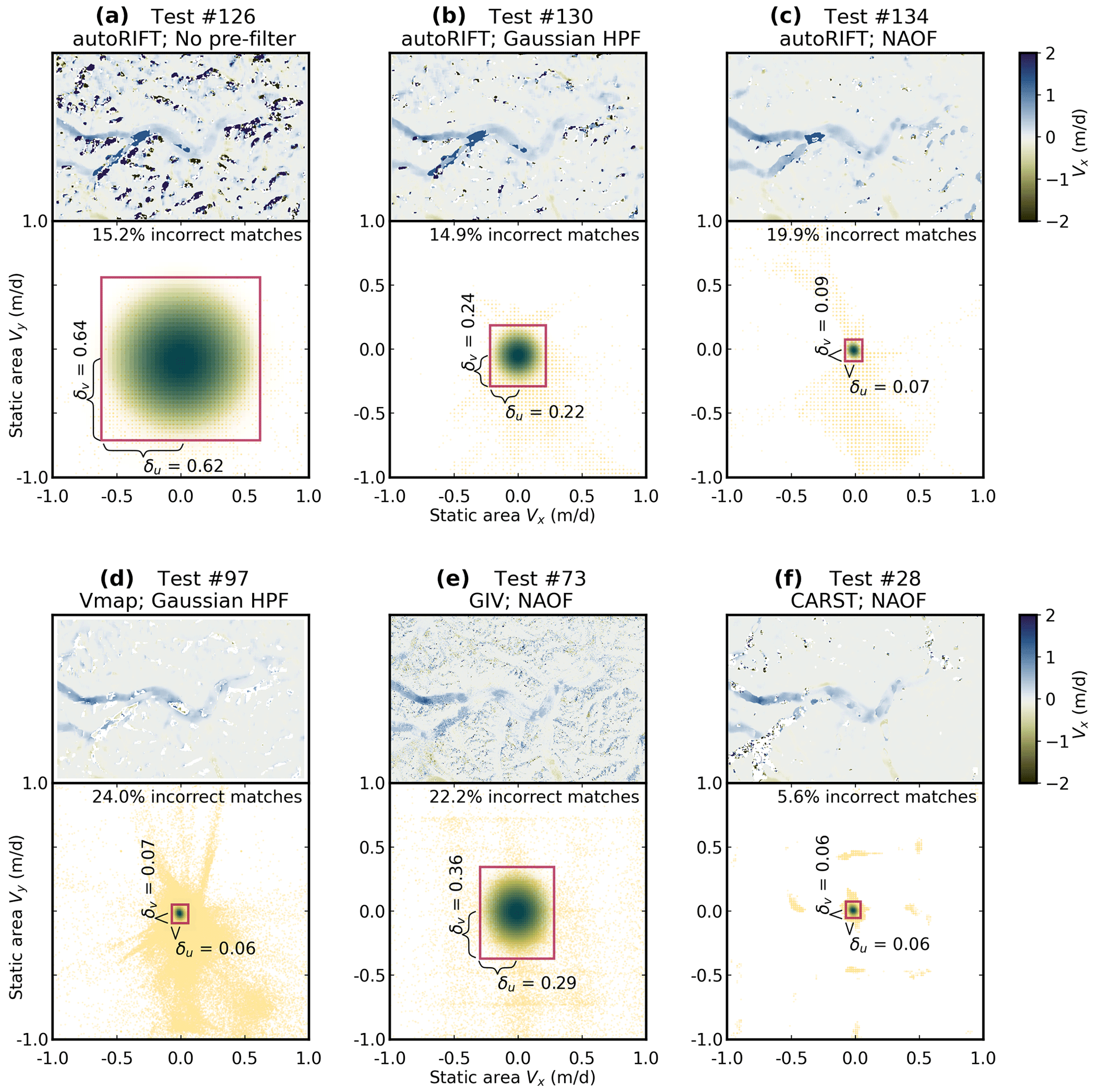
Figure 2 Feature-tracking results and static area velocities for the Landsat 8 pair 2018-03-04–2018-04-05 using six different parameter sets. Each subpanel includes a map of the east–west velocity component (V_x) at the top and the distribution of static-terrain velocities (yellow dots) with their kernel density estimate (KDE) at the bottom. The red box indicates the boundary where KDE drops to $\mathrm{1}/e^{\frac{z^{\mathrm{2}}}{\mathrm{2}}}$ of the peak KDE reading. Measurements falling outside the red box are labeled as incorrect matches, with the ratio to the total number of static area measurements shown on the plot. The half-width and height of the box are assigned as δ_u and δ_v, respectively, with their value shown in the plot. (a–c) Sample tests derived using autoRIFT with different prefilters. (d–f) Sample tests derived using vmap, GIV, and CARST, respectively. See Table S1 for the full parameters corresponding to each test.

Unlike the static terrain velocities, the along-flow strain rate does not show characteristic spatial variability across most tests; these values tend to form a single cluster centered on zero (Fig. 3 bottom panels; also Figs. S17–S24). The variability in the normal and shear strain rates is similar, as indicated by similar ${\mathit{\delta }}_{x^{\prime }{x}^{\prime }}$ and ${\mathit{\delta }}_{x^{\prime }{y}^{\prime }}$ values. This suggests that random noise, not glacier physics, controls such variability. The magnitude of ${\mathit{\delta }}_{x^{\prime }{y}^{\prime }}$ (Metric 2) does not show an obvious correlation to the velocity map (Fig. 3 upper panels), but a closer inspection by plotting the overall strain rate magnitude ($\sqrt{{\dot{\mathit{ϵ}}}_{x^{\prime }{x}^{\prime }}^{\mathrm{2}}+{\dot{\mathit{ϵ}}}_{x^{\prime }{y}^{\prime }}^{\mathrm{2}}}$) shows that ${\mathit{\delta }}_{x^{\prime }{y}^{\prime }}$ relates to the smoothness of the strain rate map (Fig. 3 middle panels). Metric 2 is insensitive to correlated error over long spatial scales (Fig. 3c) but is sensitive to high-frequency spatial variation with small amplitude (Fig. 3a). The ${\mathit{\delta }}_{x^{\prime }{y}^{\prime }}$ and ${\mathit{\delta }}_{x^{\prime }{x}^{\prime }}$ values range from 0.001 to 0.12 d⁻¹ across the 172 velocity maps (Figs. S17–S28 and Table S2).

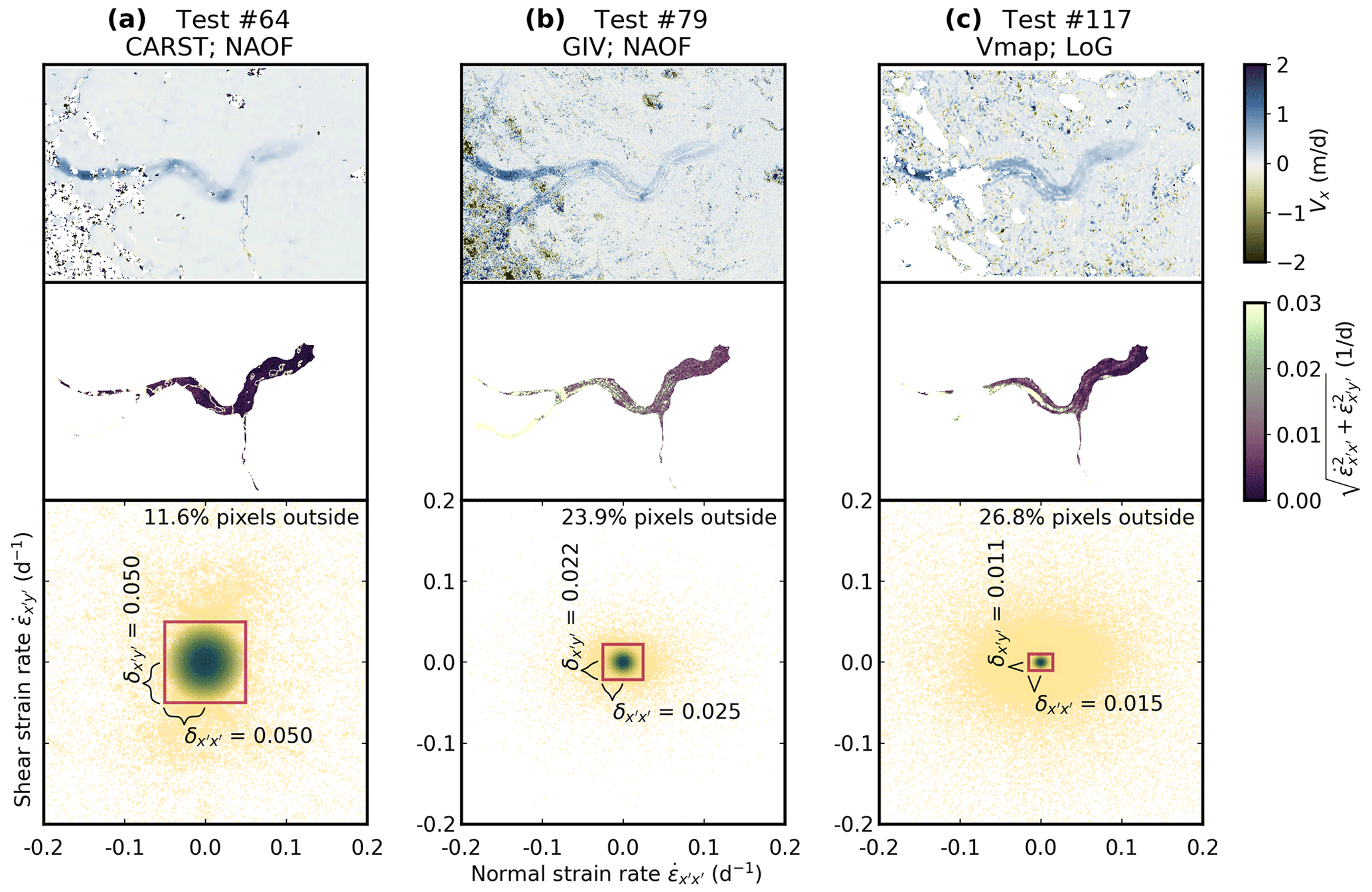
Figure 3 Feature-tracking results and flow strain rate of the Landsat 8 pair 2018-08-02–2018-08-18 using three different parameter sets. Each subpanel includes a map of the east–west velocity component (V_x) at the top, map of strain rate magnitude in the middle, and scatterplot showing the strain rate distribution (yellow dots) with their kernel density estimate (KDE) at the bottom. The red box indicates the boundary where KDE drops to $\mathrm{1}/e^{\frac{z^{\mathrm{2}}}{\mathrm{2}}}$ of the peak KDE reading. The half-width and height of the box are assigned as ${\mathit{\delta }}_{x^{\prime }{x}^{\prime }}$ and ${\mathit{\delta }}_{x^{\prime }{y}^{\prime }}$, respectively, with their value shown in the plot. See Table S1 for the full parameters corresponding to each test number.

3.2.1 Relationship between the metrics, tracking parameters, and velocity map quality

As expected, the values of Metric 1 (δ_u) and Metric 2 (${\mathit{\delta }}_{x^{\prime }{y}^{\prime }}$) vary across the 172 tests depending on multiple parameter selections. For example, when the satellite images are high-pass filtered before computing the cross-correlation surface, the resulting velocity maps often display improved quality as represented by a low δ_u value (Fig. 4a). This observation aligns with several past studies (Dehecq et al., 2015; Fahnestock et al., 2016; Van Wyk de Vries and Wickert, 2021). The δ_u values also decrease with increasing matching template size, a classic trade-off between spatial smoothing and noise (Ahn and Howat, 2011, Fig. 4b).

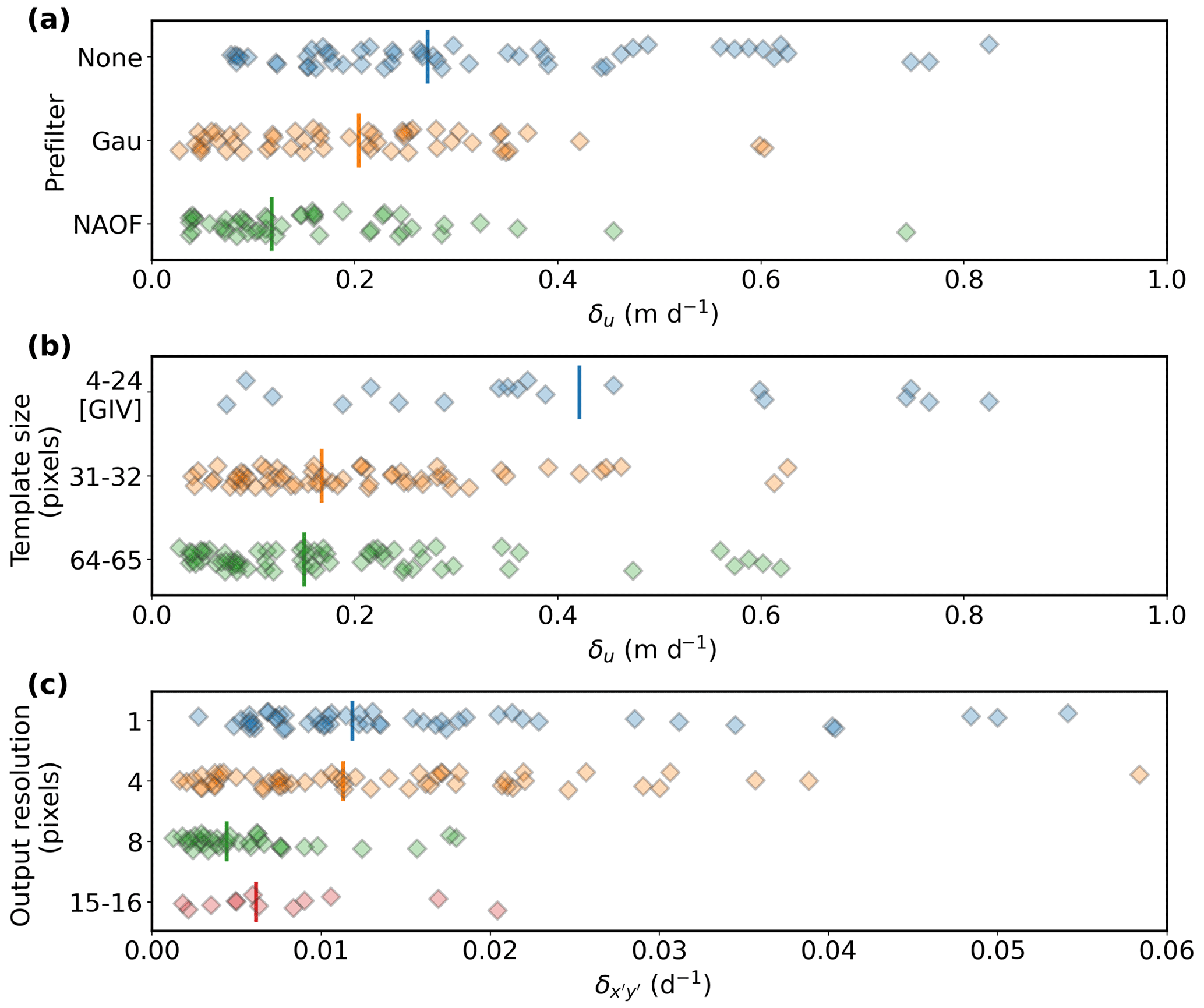
Figure 4 Relationship between selected velocity map generation parameters and our velocity map quality metrics. Each panel is a one-dimensional scatter plot showing different parameter choices used during the feature-tracking process versus the derived metric. Each point represents a different test result. Vertical bar indicates the median value of each subgroup. (a) Prefilter versus δ_u (Metric 1). (b) Matching template size versus δ_u (Metric 1). See the description of GIV in Methods for its different approach regarding the template size. (c) Output resolution versus ${\mathit{\delta }}_{x^{\prime }{y}^{\prime }}$ (Metric 2).

We can also see systematic variation in ${\mathit{\delta }}_{x^{\prime }{y}^{\prime }}$: it generally decreases as output velocity map resolution (pixel size) increases, with a minimum of ∼ 0.004 d⁻¹ (Fig. 4c). Substituting representative values for Kaskawulsh Glacier into Eq. (14) (H=700 m (Foy et al., 2011), Y=3500 m, ${\overline{u}}_{x^{\prime }}=\mathrm{0.3}$ m d⁻¹, and ${\overline{u}}_{\mathrm{b}}=\mathrm{0}$ m d⁻¹), we obtain a recommended value of 0.004 d⁻¹ for ${\mathit{\delta }}_{x^{\prime }{y}^{\prime }}$. Note that we assume no basal slip in this calculation, which may not be physically realistic for Kaskawulsh Glacier and likely yields an overestimated ${\mathit{\delta }}_{x^{\prime }{y}^{\prime }}$ recommendation. Nevertheless, these two independent computations suggest that, in our case, velocity maps with an output grid cell size equal to or larger than 8 times the input pixel size should have better quality because the observed strain rate is constrained by glacier physics. On the other hand, the observed strain rate in velocity maps with a finer output grid cell size of 1 times or 4 times the input pixel size should be dominated by large feature matching uncertainty.

A combined analysis of the two metrics offers a more powerful quality indicator for glacier velocity maps. Maps with higher δ_u and ${\mathit{\delta }}_{x^{\prime }{y}^{\prime }}$ values tend to have fewer correct matches (Fig. 5a). Again, the recommended value of ${\mathit{\delta }}_{x^{\prime }{y}^{\prime }}$ based on glacier physics (0.004 d⁻¹ for Kaskawulsh, Eq. 14) seems to play an important role. All the maps with ${\mathit{\delta }}_{x^{\prime }{y}^{\prime }}$ less than this threshold value have at least 50% correct matches (Fig. 5a). These results strongly support the hypothesis that the uncertainty of correct matches depends on the prominence of the cross-correlation peak.

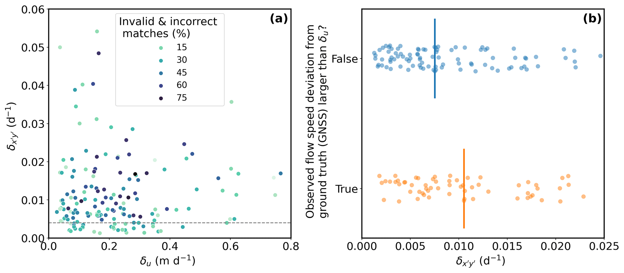
Figure 5 Relationship between our metrics and velocity map quality. (a) Values for ${\mathit{\delta }}_{x^{\prime }{y}^{\prime }}$ (Metric 2) versus δ_u (Metric 1) for all 172 tests, with point color showing the percentage of invalid (as NODATA pixels) and incorrect matches in the corresponding output velocity map. Dashed gray line indicates where ${\mathit{\delta }}_{x^{\prime }{y}^{\prime }}=\mathrm{0.004}$ d⁻¹ (see text). (b) One-dimensional scatter plot showing observed flow speed deviation from the ground truth (GNSS) versus ${\mathit{\delta }}_{x^{\prime }{y}^{\prime }}$ (Metric 2). The deviation is grouped by whether it is larger than the inferred uncertainty of correct matches (δ_u; Metric 1). Vertical bars represent the median values of the corresponding groups.

3.2.2 Comparison with in situ measurements and synthetic offset test

We find that a considerable number of velocity maps (73 out of 172) have speed deviation (in the V_x component) from the GNSS ground truth data larger than their δ_u, the 2σ uncertainty over static terrain (Fig. 5b). Maps with higher ${\mathit{\delta }}_{x^{\prime }{y}^{\prime }}$ are more likely to show this deviation. In fact, the deviation cannot simply be explained by the inclusion of incorrect matches, which should only be around 6 %–24 % according to Fig. 2 and Table S2. We argue that this deviation is related to the fact that correct matches on the glacier surface have a different noise distribution than those on the static terrain, potentially related to differences in the local variance of surface topography (roughness) and reflectance (texture) between static and ice surfaces (Paul et al., 2017). The synthetic offset test results (Sect. 3.1.4) support this hypothesis, with more spurious matches and noise observed on the glacier surface compared to the static terrain (Fig. 6). This finding suggests that correct matches on the glacier surface inherently have larger uncertainty.

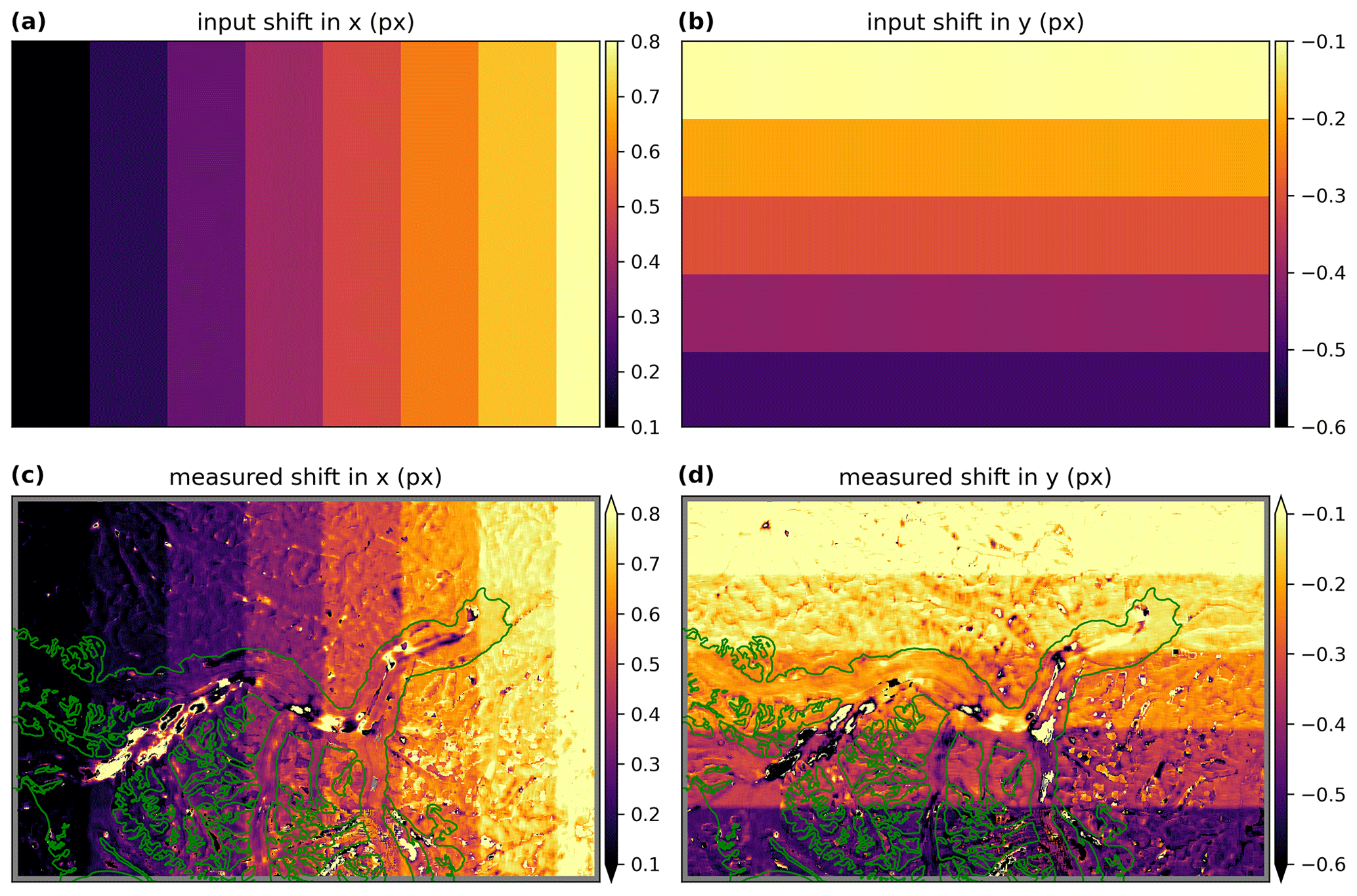
Figure 6 Feature-tracking tests using synthetic offset fields (Sect. 3.1.4). (a, b) The x and y components of the synthetic offset field applied to a single Landsat 8 image acquired on 2018-03-04 (Table 1). (c, d) Feature-tracking results (vmap, kernel size = 35 px, parabolic subpixel refinement) show a larger deviation on Kaskawulsh Glacier surface (green polygons) than the static areas.

4 Discussion

The correct-match uncertainty (δ_u and δ_v) is theoretically smaller than the bulk variability (e.g., standard derivation) computed from mixed correct and incorrect matches, which is true for the data evaluated in this study. For example, each ITS_LIVE scene-pair glacier velocity map for Kaskawulsh Glacier during 2018 is distributed with an internally calculated standard deviation of static terrain velocities as uncertainty. These 2σ errors are larger than the corresponding δ_u or δ_v values (Fig. 7 for V_x; see Sect. 3.1.3 for details). Since the uncertainty of incorrect matches is large and unpredictable, we argue that only correct-match uncertainty should be considered when evaluating velocity map quality.

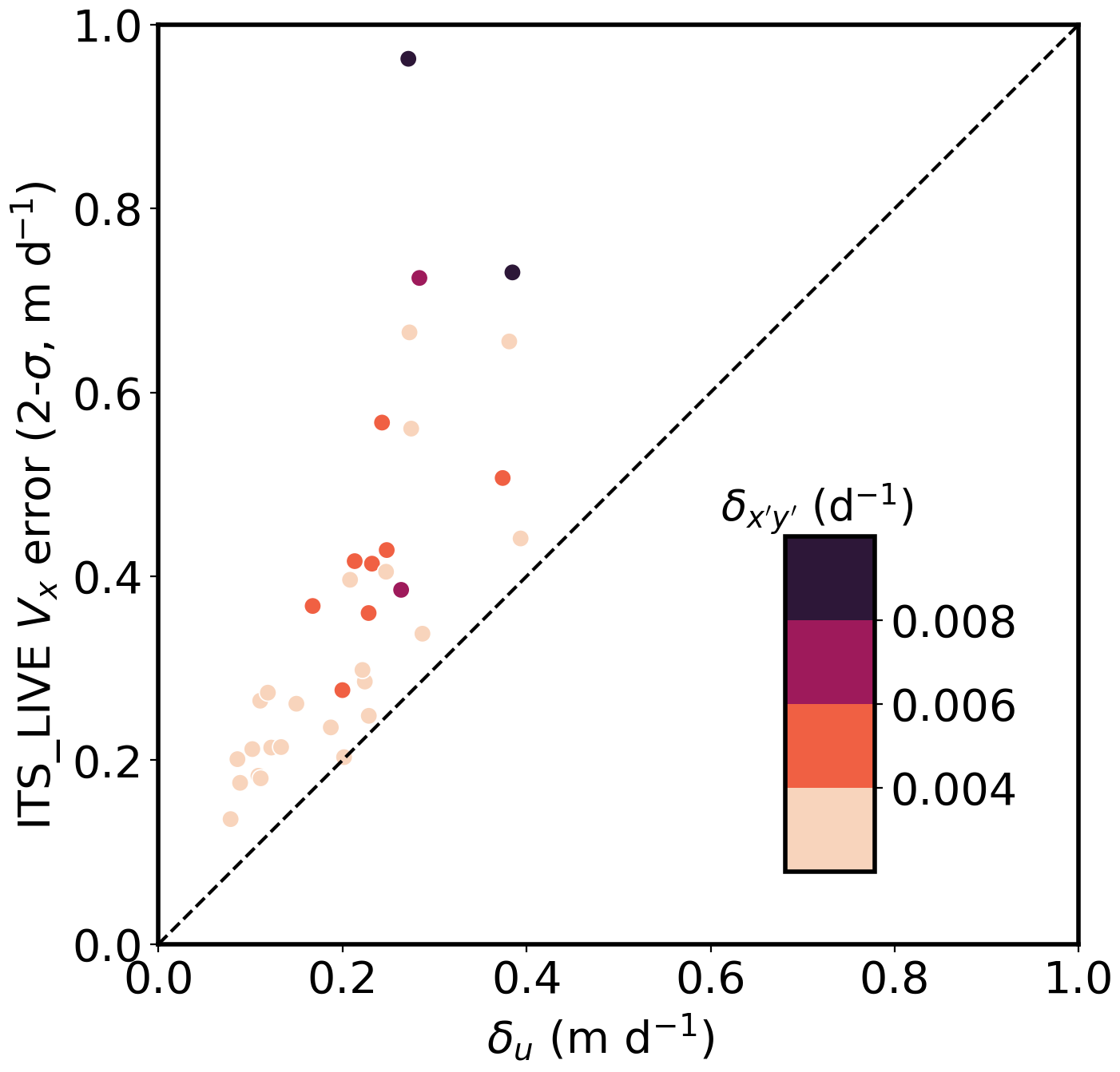
Figure 7 Comparison of reported ITS_LIVE V_x error (2 times the Vx_err value from original metadata) with our derived correct-match δ_u uncertainty (Metric 1) for 35 velocity maps. Each point represents a scene pair listed in Table S3, with color showing the corresponding uncertainty of the glacier shear strain rate (Metric 2). The dashed line indicates the 1:1 ratio of the two axes. Data used to prepare this figure are available in Table S4.

Although δ_u and δ_v are good quality indicators, they are not good estimators for the uncertainty of the ice velocity. This is because (1) ice velocities also contain incorrect matches and (2) ice velocities have a different noise distribution than static terrain velocities (Fig. 6). Attempts using static area velocity statistics to assign ice-velocity uncertainty are likely to show many outliers when compared with ground truth data (e.g., Fig. 5b in this study and Fig. 6 of Redpath et al., 2013). Nevertheless, minimizing δ_u and δ_v is still important because low correct-match uncertainty relates to low bulk variability (Fig. 6) and reduces the chance of an invalid or incorrect match (Fig. 5a). It is also worth examining the pattern of incorrect matches discovered during the same workflow (Fig. 2) for efficient mitigation.

The variability in flow strain rate provides a second way to assess the quality of glacier velocity maps. Larger ${\mathit{\delta }}_{x^{\prime }{y}^{\prime }}$ correlates to more bad matches (Fig. 5a), leading to lower overall accuracy (Fig. 5b) and a higher bulk uncertainty (Fig. 7). It is thus essential to ensure that the velocity map has certain spatial coherence to minimize ${\mathit{\delta }}_{x^{\prime }{y}^{\prime }}$ until it decreases to a suggested value based on ice flow physics (Eq. 14). Without spatial smoothing, it may not be possible for ${\mathit{\delta }}_{x^{\prime }{y}^{\prime }}$ to go below that threshold value (Fig. 4c). Velocity maps with ${\mathit{\delta }}_{x^{\prime }{y}^{\prime }}$ near the threshold value theoretically have a coherent, less error-prone, and physically meaningful strain rate field, which is critical for glacier modeling.

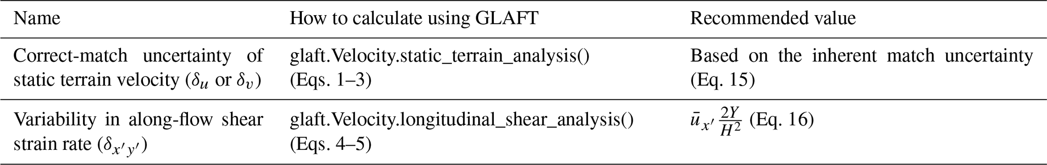
4.1 Recommended strategy to evaluate velocity map quality

The metrics presented in this paper can be used to assess the quality of glacier velocity maps (Table 2). We suggest that the correct-match uncertainty of static terrain velocity, δ_u (and δ_v if the map is derived using a non-square matching template, which is common for SAR feature tracking), should be as low as possible until the value reflects the inherent match uncertainty only. If the inherent match uncertainty (2σ) is 0.2 pixels (Sciacchitano, 2019), the desired range of δ_u is

$$\begin{array}{}\text{(15)}& {\mathit{\delta }}_u\le \mathrm{0.2}\times {\displaystyle \frac{\text{pixel size of source images}}{\text{duration of source image pair}}}.\end{array}$$

The recommended value for the variability in along-flow shear strain rate, ${\mathit{\delta }}_{x^{\prime }{y}^{\prime }}$, depends on the flow-law parameter n and basal sliding velocity ${\overline{u}}_{\mathrm{b}}$ (Eq. 14), which can be challenging to measure. However, based on the test results presented in this study, proposing an overestimated value by setting zero basal slip may be acceptable because it is more conservative on whether the observed strain rate field links to the actual ice flow dynamics. With the general assumption of n=3, we suggest the following guideline for setting a ${\mathit{\delta }}_{x^{\prime }{y}^{\prime }}$ threshold, which relates to the average surface along-flow speed ${\overline{u}}_{x^{\prime }}$, channel half-width Y, and average ice thickness H:

$$\begin{array}{}\text{(16)}& {\mathit{\delta }}_{x^{\prime }{y}^{\prime }}\approx {\overline{u}}_{x^{\prime }}{\displaystyle \frac{\mathrm{2}Y}{H^{\mathrm{2}}}}.\end{array}$$

Table 2 Summary of using static terrain velocities and along-flow strain rates to assess glacier velocity maps.

We can apply these metrics and guidelines in various use cases. Users who run feature-tracking workflows can compute these metrics for their output velocity maps. If either metric deviates from the recommended range, they can try a different parameter combination, including prefilters, tracking parameters, subsampling, masking, and other postprocessing steps, until the metrics fall within the recommended values. In addition to these metrics, the users can analyze the number and spatial distribution of incorrect matches over the static terrain to identify directions of improvement; see Fig. 2 and discussion in Sect. 3.2 for an example. These metrics will also serve as a basis for comparing novel feature-tracking algorithms (e.g., Altena and Kääb, 2020) with traditional algorithms. Glacier modelers can use these metrics to select the best possible velocity maps to derive physical quantities (such as strain rate) with minimal error propagation. When a velocity map has a ${\mathit{\delta }}_{x^{\prime }{y}^{\prime }}$ much larger than the suggested value, one can select an appropriate smoothing level for the velocity map and recalculate ${\mathit{\delta }}_{x^{\prime }{y}^{\prime }}$ until it reaches the suggested value. Finally, we recommend that data producers calculate these metrics (with the help of the GLAFT package) and include them in the metadata associated with each velocity product. This will enable users to assess product quality and determine if customized velocity maps are required for their applications.

To estimate the uncertainty of ice flow velocity, Metric 1 (δ_u or δ_v) seems to be a plausible option and has been used in many studies (see Sect. 2.1). However, on-ice velocities likely have a different noise distribution than off-ice velocities, and the use of Metric 1 as the flow uncertainty will be sub-optimal. Since Metric 2 (${\mathit{\delta }}_{x^{\prime }{y}^{\prime }}$) describes the spatial variability in the flow velocity, it can potentially offer an alternative uncertainty estimator. While the latter is one of the future goals of this project, at this time, we suggest that users should treat Metric 1 as a very conservative image-wide uncertainty of the ice flow velocity.

Finally, the strategy outlined here is based on our analysis using optical images for one glacier. We expect that these metrics will also work for SAR feature tracking and different glacier settings, but additional care might be necessary. For example, SAR images typically have different range and azimuth resolutions, which could result in a significant difference between δ_u and δ_v. Also, it can be difficult to calculate both metrics over an ice sheet where there is no static terrain and limited differential velocity within a single scene. We will continue to address these issues in future GLAFT applications.

4.2 Open-source tools for computing quality metrics

The open-source GLAcier Feature Tracking testkit (GLAFT; Zheng et al., 2023a) Python package accompanying this paper can be used to compute and evaluate these metrics and associated thresholds for arbitrary input velocity map data. GLAFT contains modules for deriving and visualizing the two metrics from velocity maps generated by most feature-tracking tools. GLAFT is available on Ghub (Sperhac et al., 2021, https://theghub.org/resources/glaft, last access: 21 August 2020) for cloud access and can be installed locally via PyPI, Python's official third-party package repository and manager (https://pypi.org/project/glaft, last access: 21 August 2020). The GLAFT source code, Notebook examples, and documentation are hosted on GitHub (https://github.com/whyjz/GLAFT), with Binder-ready Jupyter Book pages (Project Jupyter et al., 2018; Executable Books Community, 2020) at https://whyjz.github.io/GLAFT/ (last access: 21 August 2020) as the Supplement of this paper.

5 Conclusions

With the release of GLAFT and the strategy outlined in Table 2 to assess glacier velocity products, we anticipate that the Earth and Environmental Science community can quickly take advantage of the findings of this study. Our work sets up the first open-source benchmarking procedure for future large-scale intercomparison exercises (such as Boncori et al., 2018) that comprise multiple image sources and various feature-tracking workflows. With proper adjustments for the physics-based metrics, these methods can be applied to study different physical processes, such as dune migration or fault displacement. The GLAFT enables the cryospheric sciences and natural hazards communities to leverage the rich glacier velocity data now available, whether they are sourced from public archives or prepared using one of the excellent open-source feature-tracking packages featured in this study.