Reconciling ice dynamics and bed topography with a versatile and fast ice thickness inversion

We present a novel thickness inversion approach that leverages satellite products and state-of-the-art ice flow models to produce distributed maps of sub-glacial topography consistent with the dynamic state of a given glacier. While the method can use any complexity of ice flow physics as represented in ice dynamical models, it is computationally cheap and does not require bed observations as input, enabling applications on both local and large scales. Using the mismatch between observed and modelled rates of surface elevation change ($\mathrm{d}h/\mathrm{d}t$) as the misfit functional, iterative point-wise updates to an initial guess of bed topography are made, while mismatches between observed and modelled velocities are used to simultaneously infer basal friction. The final product of the inversion is not only a map of ice thickness, but is also a fully spun-up glacier model that can be run forward without requiring any further model relaxation. Here we present the method and use an artificial ice cap built inside a numerical model to test it and conduct sensitivity experiments. Even under a range of perturbations, the method is stable and fast. We also apply the approach to the tidewater glacier Kronebreen on Svalbard and finally benchmark it on glaciers from the Ice Thickness Models Intercomparison eXperiment (ITMIX, Farinotti et al., 2017), where we find excellent performance. Ultimately, our method shown here represents a fast way of inferring ice thickness where the final output forms a consistent picture of model physics, input observations and bed topography.

1 Introduction

Knowledge of the ice thickness of glaciers is crucial for a range of applications, from fieldwork planning to water management, and ultimately for projections of expected sea level rise in the face of climate warming (Oppenheimer et al., 2019; Rounce et al., 2023). Ice thickness not only determines the ice volume of a glacier, but the sub-glacial topography is furthermore a key control on future retreat of glaciers. As such, accurate bed maps are instrumental in initializing prognostic simulations of numerical ice flow models with the correct boundary conditions.

Ice thickness can be established using geophysical methods such as ground-penetrating radar (Bogorodsky et al., 1985). However, observations are only dense along their acquisition lines, while considerable spacing between lines is the norm. To produce distributed maps of ice thickness, statistical techniques have been developed to interpolate between observations (Flowers and Clarke, 1999; Fretwell et al., 2013; Neven et al., 2021). However, only a small fraction of glaciers worldwide have any thickness observations at all (Welty et al., 2020).

As an alternative to field measurements, inversion techniques have been introduced that allow the derivation of a bed estimate from easily obtainable surface observations alone. Early works include the use of scaling relationships that allow the computation of mean bed elevation from surface area (i.e. volume–area scaling, Chen and Ohmura, 1990; Bahr et al., 1997, 2014). More advanced approaches apply computational methods relying on a physical understanding of how ice flows, often (when available) in conjunction with measured ice thicknesses. The underlying rationale is that easily observable surface characteristics, such as the surface elevation height, are a product of the external climate forcing (e.g. climatic mass balance), ice dynamics and sub-glacial topography, and therefore an inference about the latter can be made from knowledge of the former. Recent years have seen an increasing number of such new ice thickness inversion approaches; an overview of widely used methods is given in Farinotti et al. (2017, 2021). The large majority of approaches follow at least one of the two strategies: in the first one, the physical calculations of ice dynamics underpinning the inversion are conducted along flow lines or at randomly selected points on a glacier, and subsequently the results are extrapolated to surrounding areas, often while taking into account some first-order glaciological principles, e.g. the strong link between surface slope and ice thickness (Farinotti et al., 2009; Linsbauer et al., 2009; Huss and Farinotti, 2012; Li et al., 2012; Linsbauer et al., 2012; Paul and Linsbauer, 2012; Clarke et al., 2013; Frey et al., 2014; Brinkerhoff et al., 2016; Rabatel et al., 2018; Maussion et al., 2019; Werder et al., 2020). This is computationally efficient as compared to calculating distributed ice thickness fields but comes with the limitation that the physics-based inversion is only conducted at specific locations. In the second approach, a simple model considering only internal shear (i.e. the shallow ice approximation, SIA) is applied to turn a modelled or observed quantity (e.g. depth-integrated ice flux or surface velocities) into ice thickness, which is sometimes complemented by a parameterization for basal sliding (Farinotti et al., 2009; Huss and Farinotti, 2012; Li et al., 2012; Linsbauer et al., 2012; Paul and Linsbauer, 2012; Clarke et al., 2013; Frey et al., 2014; Gantayat et al., 2014; Fürst et al., 2017; Rabatel et al., 2018; Langhammer et al., 2019; Maussion et al., 2019; Werder et al., 2020; Zorzut et al., 2020; Millan et al., 2022a). These approaches are also computationally cheap compared to calculations based on a higher-order or full Stokes model, and they exploit the simple mathematical nature of the depth-integrated SIA. However, the simplifying assumptions about ice dynamics that are at the heart of the SIA (e.g. entirely local stress balance, ice flow strictly downhill) translate into errors in the calculated ice thicknesses at locations where the conditions are not met. Although different in their complexities, their required inputs and their strengths and limitations (for more details, the reader is referred to the respective publications), the thickness inversion approaches discussed here, share limitations that arise from following one or both of the mentioned strategies. For instance, using a bed derived with such methods for prognostic simulations with map-plane higher-order or full Stokes models causes artefacts in the forward simulation as a result of an ice thickness field that is not consistent with ice flow dynamics. To mitigate such errors, models are typically run with constant boundary conditions prior to the prognostic simulation (called model relaxation), which, however, often results in a glacier state significantly different from observations (Schlegel et al., 2015).

A different approach was presented by van Pelt et al. (2013), building on previous work in the context of inversion problems in fluid mechanics (Heining, 2011). Using historical observations of external forcing and starting from an initial guess for bed topography, they use the Parallel Ice Sheet Model (PISM) (Bueler and Brown, 2009) to simulate centuries of glacier evolution up until the present day, when a comparison between modelled and observed surface elevations is made. Based on the assumption that any deviations between the two are due to errors in the bed, this mismatch is then used to update the sub-glacial topography. These two steps are repeated iteratively until a certain stopping criterion is reached. This approach allows the inclusion of any physics that state-of-the-art ice flow models feature, and it results in a distributed map of bed topography that is in balance with the present-day dynamic state of the glacier and the external forcing. For ensuing prognostic simulations, no relaxation is needed as all input parameters and physics used for the forward simulations can also be used in the thickness inversion.

The approach by van Pelt et al. (2013) is based on the idea that the present-day dynamic state of a glacier is best reproduced by simulating that glacier for centuries up until today using historical forcing. However, such forcing data are rarely available and are subject to considerable uncertainties. Furthermore, due to the long time spans modelled, the approach is computationally costly. Here, we exploit the fact that the instantaneous rate of surface elevation change $\mathrm{d}h/\mathrm{d}t$, which also represents the dynamic state of a glacier, is much faster to model, allowing us to apply a similar methodology to van Pelt et al. (2013) while only requiring a fraction of the computational resources. In our new approach, we furthermore extend the capabilities of the thickness inversion in that we simultaneously infer basal friction using observed surface velocities akin to a previously published approach (Pollard and DeConto, 2012). Ultimately, we establish a framework that is able to provide a comprehensive view of the state of a glacier consistent with its external forcing, its ice dynamics and its bed topography while being at a low computational cost. Allowing us to choose between different levels of complexity for the ice flow physics and whether or not to simultaneously infer basal friction, our approach is suitable both for detailed inversions at the local scale as well as for fast large-scale applications.

In the following, we describe our new fast ice thickness inversion approach using PISM as a forward model. We demonstrate its capabilities with an example of an artificial ice cap grown inside a numerical model and apply and test it on the tidewater glacier Kronebreen on Svalbard. Finally, benchmark experiments on three glaciers from the Ice Thickness Models Intercomparison eXperiment (ITMIX, Farinotti et al., 2017) are conducted.

2 A new thickness inversion approach

2.1 Inverse method

2.1.1 Bed inversion

The general functional principle derives from the idea that a numerical model of a glacier initialized with the correct boundary conditions should behave similarly to a real glacier; if not, one needs to conclude that the model setup is erroneous in some way. In a simple case without basal sliding and, neglecting thermodynamic processes, the first-order controls on ice dynamics are the climatic mass balance, the glacier surface shape and the bed. By assuming that it is possible to set up a numerical ice flow model where all of these inputs are sufficiently well represented except for bed topography (because they are surface observations), we may attribute any differences in modelled vs. observed ice geometry and dynamics to origins from errors in the bed.

To turn this framework into an inversion approach, the following workflow is applied (Fig. 1). First, a numerical representation of a glacier is set up inside an ice flow model with observations of surface shape from a digital elevation model (DEM) and climatic mass balance. Furthermore, some arbitrary bed shape is assumed. For instance, it is straightforward to derive a rough bed estimate from a DEM with the perfect-plasticity method (Nye, 1952; Haeberli and Hoelzle, 1995). As Habermann et al. (2012) point out, though, an initial bed guess should not contain roughness not justified by the input data, so some smoothing, e.g. with a Gaussian filter, may be in order.

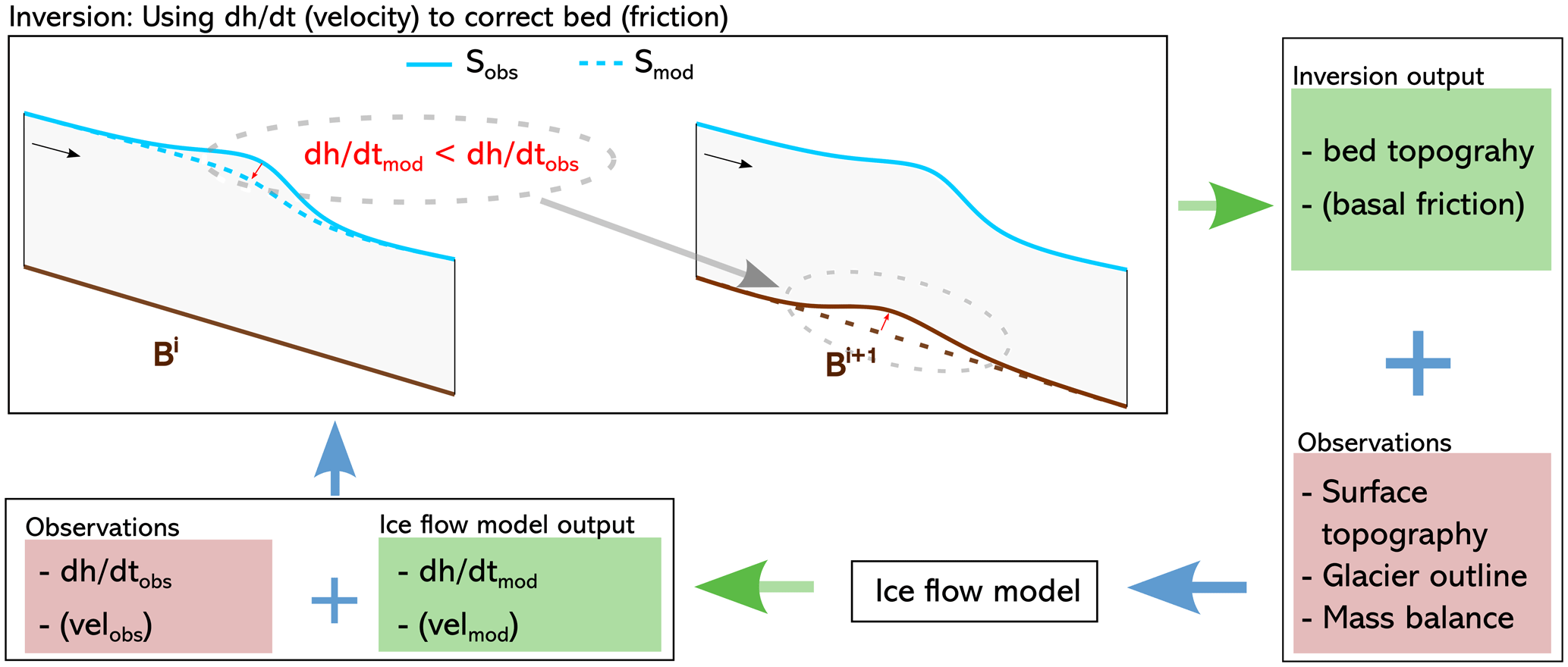
Figure 1 Schematic representation of the thickness inversion workflow where observations and output from an ice flow model are used together to iteratively correct the bed. The example here shows a negative $\mathrm{d}h/\mathrm{d}t$ misfit (Eq. 7) resulting in a bed uplift, but the same logic applies for a positive $\mathrm{d}h/\mathrm{d}t$ misfit resulting in a corresponding bed lowering. During a friction update an analogous iteration is performed but using the velocity misfit (Eq. 2) and applying changes to the basal friction field.

Then, the ice flow model is run forward with the goal of comparing whether modelled and observed ice dynamics agree. As described before, the target variable here is the rate of surface elevation change $\mathrm{d}h/\mathrm{d}t$ as a measure of the dynamic state of the glacier. From the model side, this requires only a stress balance simulation or a simulation with a short timescale length dt to compute the instantaneous $\mathrm{d}h/\mathrm{d}{t}_{\text{mod}}$. From the observational side, this requires either an already existing $\mathrm{d}h/\mathrm{d}t$ product (e.g. Hugonnet et al., 2021) or two DEMs from different years, where it is assumed that the rate of surface elevation change between them is constant, allowing the derivation of the quantity $\mathrm{d}h/\mathrm{d}{t}_{\text{obs}}$. If $\mathrm{d}h/\mathrm{d}{t}_{\text{mod}}=\mathrm{d}h/\mathrm{d}{t}_{\text{obs}}$, it is reasonable to conclude that the bed topography is correct, because the model correctly reproduces the observations. However, in the more likely event that they are not equal, the differences between the two are ascribed to origins from errors in the bed, following the logic discussed above.

If there is a mismatch between modelled and observed quantities, previous work has shown that point-wise updates can be applied to the unknown parameter (in this case bed topography) as a simple function of that mismatch (van Pelt et al., 2013; Michel et al., 2013; Heining, 2011; Pollard and DeConto, 2012). Here, a new bed Bⁱ⁺¹ is hence produced by subtracting, at any point in space in the domain, the misfit in modelled vs. observed $\mathrm{d}h/\mathrm{d}t$ at that point from the present bed Bⁱ, such that

$$\begin{array}{}\text{(1)}& B^{i+\mathrm{1}}=B^i-\mathit{\beta }\left({\displaystyle \frac{\mathrm{d}{h}_{\text{mod}}^i}{\mathrm{d}t}}-{\displaystyle \frac{\mathrm{d}{h}_{\text{obs}}}{\mathrm{d}t}}\right),\end{array}$$

where β is a scalar that controls the magnitude of bed corrections. These simple steps described here (running the model forward, computing the misfit in modelled vs. observed $\mathrm{d}h/\mathrm{d}t$ and updating the bed) are repeated iteratively until a satisfactory solution for the bed is found (Fig. 1). Note that van Pelt et al. (2013) used a similar equation, although, instead of $\mathrm{d}h/\mathrm{d}t$, the modelled surface elevation S_mod after century-long time-dependent runs was used to calculate a misfit with the observed surface S_obs, requiring much greater computational resources.

2.1.2 Friction inversion

The method as presented above works well under the assumption that sliding is not significant. Where this simplification does not hold, one solution is to prescribe some friction field. However, this makes the modelled ice thickness dependent on an often poorly constrained parameter, which could lead to considerable errors in the recovered bed. Here, we address this issue by inverting for basal friction following a similar methodology to Pollard and DeConto (2012) and Le clec'h et al. (2019). Most sliding laws have a parameter (often termed friction coefficient, yield stress, etc.) that varies in space but is constant in time, which controls the strength of the sub-glacial material and hence the amount of sliding. We invert for this parameter F in a similar fashion to shown before. Specifically, an initial guess for F is made again that is subsequently updated, this time however using a mismatch in modelled vs. observed ice flow speed u, such that

$$\begin{array}{}\text{(2)}& {\displaystyle }{F}^{i+\mathrm{1}}=\left\{\begin{array}{ll}{F}^i-\mathit{\lambda }{F}^i& \text{if }\frac{u_{\text{mod}}^i-u_{\text{obs}}}{u_{\text{obs}}}<-\mathit{\lambda },\\ F^i+\mathit{\lambda }{F}^i& \text{if }\frac{u_{\text{mod}}^i-u_{\text{obs}}}{u_{\text{obs}}}>\mathit{\lambda },\\ F^i+F^i\left(\frac{u_{\text{mod}}^i-u_{\text{obs}}}{u_{\text{obs}}}\right)& \text{otherwise.}\end{array}\right.\end{array}$$

The parameter λ serves to prevent too-strong updates to the friction field. Importantly, bed and friction are not updated in the same iteration. This is because the $\mathrm{d}h/\mathrm{d}t$ misfit and the velocity misfit both represent a mismatch in modelled vs. observed flow dynamics, and it is not clear how to disentangle which part of that mismatch is due to an erroneous friction field vs. an erroneous bed. Indeed, our experiments confirm that the method does not converge with simultaneous bed and friction updates in each iteration. So, instead, F is only updated once after the model has converged to a solution for ice thickness. At that point, a model configuration that can explain $\mathrm{d}h/\mathrm{d}{t}_{\text{obs}}$ is found. However, only if that model also explains observed surface speed is it reasonable to conclude that the imposed friction field is correct, assuming that the friction field is the largest remaining unknown control on ice dynamics. If there is no agreement in modelled vs. observed surface speeds, F is likely not correct (again under that same assumption) and hence the modelled bed elevation is erroneous. A change in the friction field will trigger a response of the ice dynamics, and so $\mathrm{d}h/\mathrm{d}{t}_{\text{mod}}$ will no longer match $\mathrm{d}h/\mathrm{d}{t}_{\text{obs}}$ after having updated F. Following a friction update, a new bed thus needs to be found that can explain $\mathrm{d}h/\mathrm{d}{t}_{\text{obs}}$ with that new friction field. Therefore, bed and surface updates according to Eqs. (1) and (3) again need to be applied until any $\mathrm{d}h/\mathrm{d}t$ mismatch is resolved. Subsequently, the velocity mismatch is evaluated and, if needed, F is updated. Ultimately, this alternation between many bed updates and one friction update is repeated until a combination of a bed and friction field is found that explains both $\mathrm{d}h/\mathrm{d}{t}_{\text{obs}}$ and u_obs.

2.2 Regularization using surface updates

Our experiments show that the approach described above is generally capable of recovering sub-glacial topography and basal friction. However, no ice thickness inversion, regardless of the method used, is unique because small-scale bed undulations leave no expressions on the glacier surface, and hence no statement on the existence or non-existence of such features can be made (Gudmundsson, 2003; Bahr et al., 2014). To avoid unjustified small-scale features in the recovered bed, the solution needs to be biased towards outcomes that take this limitation into account. Furthermore, real-world problems imply that input data and model physics are never perfect, meaning that not all deviations between modelled and observed dynamics can be attributed to errors in the bed.

Previous work in the spirit of traditional inversion theory has tackled these issues by introducing so-called regularization terms that force the modelled bed to be smooth and that account for a degree of imperfection in the model (Habermann et al., 2012). Here, we present a novel way of handling this issue: every time the bed topography is updated, a small proportion θ of the $\mathrm{d}h/\mathrm{d}t$ misfit is used to also update the glacier surface S in the opposite direction of the bed such that a new surface Sⁱ⁺¹ is given by

$$\begin{array}{}\text{(3)}& S^{i+\mathrm{1}}=S^i+\mathit{\theta }\mathit{\beta }\left({\displaystyle \frac{\mathrm{d}{h}_{\text{mod}}^i}{\mathrm{d}t}}-{\displaystyle \frac{\mathrm{d}{h}_{\text{obs}}}{\mathrm{d}t}}\right).\end{array}$$

Doing so results in a “squeezing” effect where an upwards correction of the bed (i.e. the ice thickness becomes smaller) results in a lowered glacier surface at that point and vice versa for a downwards bed correction. This leads to locally steeper surface slopes and therefore increased driving stresses that gently induce further bed corrections in surrounding areas, thus evening out small bed undulations. At the same time, the small changes in the surface shape allow the model to accommodate observations that it otherwise cannot reproduce, be it because of input errors or imperfect model physics. Indeed, our experiments show that the bed and surface updates interact to finally yield a configuration where $\mathrm{d}h/\mathrm{d}{t}_{\text{mod}}=\mathrm{d}h/\mathrm{d}{t}_{\text{obs}}$.

2.3 Stabilization techniques

To prevent sudden shocks in the inversion process and to aid convergence, below we present techniques that can be used to stabilize the inversion. Not all of these methods will be required for all the glaciers. Rather, the below should be considered a toolbox that can be applied variably to different setups.

• β ramp-up. The $\mathrm{d}h/\mathrm{d}t$ misfit and hence the bed corrections are generally largest at the start of the inversion and after friction updates. To stabilize the inversion, we find that it can be beneficial to scale the bed updates with a small β (Eq. 1) in those instances. Therefore, we introduce a “ramp-up” procedure where β is increased as a function of the iteration count c, such that

  $$\begin{array}{}\text{(4)}& \mathit{\beta }={\displaystyle \frac{-i_{\mathrm{s}}\cdot {\mathit{\beta }}_{\mathrm{0}}}{c+i_{\mathrm{s}}}}+{\mathit{\beta }}_{\mathrm{0}},\end{array}$$

  where β₀ is the value that β will approach asymptotically and i_s is a scaling factor determining how many iterations the ramp-up takes. After each friction update, c is reset to one.

• Ice margin treatment. At the ice margin, spurious boundary effects can occur that result from a poor representation of the ice physics there. It can therefore be advisable to interpolate the bed or the ice thickness along the glacier margins or to set them to a fixed value.

• Bed averaging. If β is too large, the bed may locally oscillate around a certain value, resulting in high-frequency noise in the bed solution. While reducing β would be a reasonable choice, it would slow down the inversion. Instead, we find that resetting the bed to a mean of the previous i_p iterations every i_p iterations can be equally effective without losing computational time.

• Input data smoothing. To avoid introducing noise present in the input data (as is often encountered in velocity observations, $\mathrm{d}h/\mathrm{d}t$ products or DEMs), a Gaussian filter can be applied to the input fields (e.g. Maussion et al., 2019).

2.4 Convergence metrics

To assess the convergence of the inversion and to validate the output against bed observations (if available), the following metrics are computed by considering all n grid points inside the ice-covered domain.

• The median (i.e. second quartile Q₂) absolute $\mathrm{d}h/\mathrm{d}t$ misfit is

  $$\begin{array}{}\text{(5)}& \left|\mathrm{\Delta }\mathrm{d}h\right|=Q_{\mathrm{2}}\left(\left|{\displaystyle \frac{\mathrm{d}{h}_{\text{mod}}}{\mathrm{d}t}}-{\displaystyle \frac{\mathrm{d}{h}_{\text{obs}}}{\mathrm{d}t}}\right|\right).\end{array}$$

• When applying friction updates, the median absolute velocity misfit is

  $$\begin{array}{}\text{(6)}& \left|\mathrm{\Delta }u\right|=Q_{\mathrm{2}}\left(\left|u_{\text{mod}}-u_{\text{obs}}\right|\right).\end{array}$$

• If bed observations are available, the mean absolute bed misfit is

  $$\begin{array}{}\text{(7)}& \stackrel{\mathrm{‾}}{\left|\mathrm{\Delta }B\right|}={\displaystyle \frac{\mathrm{1}}{n}}\sum _{\mathrm{1}}^n\left|B_{\text{mod}}-B_{\text{ref}}\right|.\end{array}$$

Note that while the above represents the metrics used in this study, it is a non-exhaustive list of possible quantities that could be computed. Based on $\left|\mathrm{\Delta }\mathrm{d}h\right|$ or a similar metric, a stopping criterion could be developed that triggers a new friction update when a certain threshold is reached. Alternatively, the number of iterations needed for model convergence can be determined based on the glacier response time (Sect. 6). In this study, we simply prescribe a fixed number of iterations between friction updates as well as the total number of iterations (Sects. 3.1 and 4.4).

2.5 Ice flow model

While the method is not bound to a specific ice flow model, we use PISM v.2.0.4 (Bueler and Brown, 2009) for the ice flow simulations. Below, we briefly present relevant aspects of PISM with respect to our thickness inversion method but refer the reader to the literature for a more in-depth description (Bueler and Brown, 2009; Winkelmann et al., 2011).

PISM allows the glaciological stress-balance equations to be solved using one of four approximations to the full Stokes equations: the SIA, the shallow shelf approximation (SSA), a hybrid SSA + SIA scheme or the Blatter–Pattyn higher-order model (Blatter, 1995; Pattyn, 2003). Any of them is suitable for the thickness inversion, but here we apply the hybrid SSA + SIA scheme. To simulate sliding, different laws are available, some of which allow interaction with modelled thermodynamics to yield values of sub-glacial water availability, which in turn determines basal friction. In this work, we do not include thermodynamic processes (Sect. 6) and rely instead on a simple pseudo-plastic power law where basal shear stress τ_b is given by

$$\begin{array}{}\text{(8)}& {\mathit{\tau }}_{\mathrm{b}}=-{\mathit{\tau }}_{\mathrm{c}}{\displaystyle \frac{\mathit{u}}{u_{\text{th}}^q|\mathit{u}{|}^{\mathrm{1}-q}}},\end{array}$$

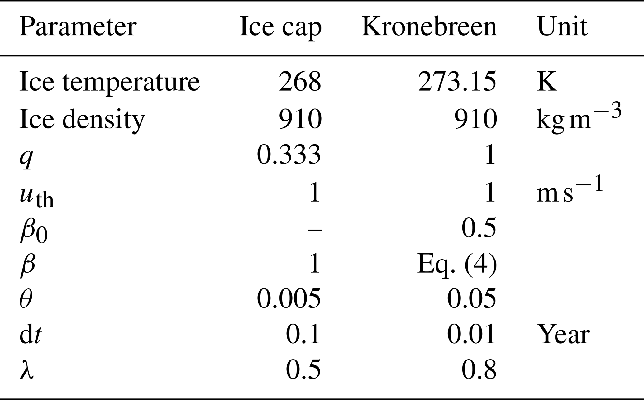
where u_th is the threshold velocity where τ_b has the same magnitude as the yield stress τ_c and $q\in [\mathrm{0},\mathrm{1}]$ is an exponent determining the plasticity of the sliding law (q=1 represents a linear sliding law). τ_c is a spatially variable constant that reflects the strength of the sub-glacial bed and hence determines the degree of sliding. This is the quantity that we invert for in Eq. (2).

3 Synthetic experiments

3.1 The synthetic ice cap

We start by using our new method on an artificial ice cap. We first design a domain with a 50×50 grid and a resolution of 2 km where we define a bed topography consisting of a flat bed including two large (500 m tall) and two small (350 m tall) bumps with a prescribed mass balance field (Fig. 2). Furthermore, we design a friction field by setting the parameter τ_c such that the left half of the domain is slippery, allowing ice to slide, while the right half is sticky, preventing any basal motion. We use a non-linear sliding law as in the MISMIP experiments (Pattyn et al., 2012) by setting the sliding law parameters $q=\mathrm{1}/\mathrm{3}$ and u_th=1 m s⁻¹ in Eq. (8) (Table 1). Subsequently, we grow the ice cap inside PISM for 10 kyr using the isothermal SSA + SIA scheme, allowing us to obtain a steady-state configuration with a maximum ice thickness of ∼1000 m. Then, we “forget” the bed and friction field and try to recover them. For the thickness inversion, we use as inputs the same mass balance as applied when growing the ice cap, the surface of the grown ice cap as well as a reference $\mathrm{d}h/\mathrm{d}{t}_{\text{obs}}$ field that is zero everywhere (since the ice cap is in steady state) and make a first bed guess assuming a completely flat bed without bumps. For the friction inversion, our first guess is that the domain is sticky everywhere, and the input required to later update this guess is the velocity field of the grown ice cap (Fig. 2). Subsequently, we simulate a short forward run with dt=0.1 years and update the bed and the ice cap surface according to Eqs. (1) and (3). In a band with a width of two cells at the ice cap margin, we set the bed elevation to zero, and we apply bed averaging every five iterations (Sect. 2.3). Using any other stabilization techniques is not found to yield further improvements.

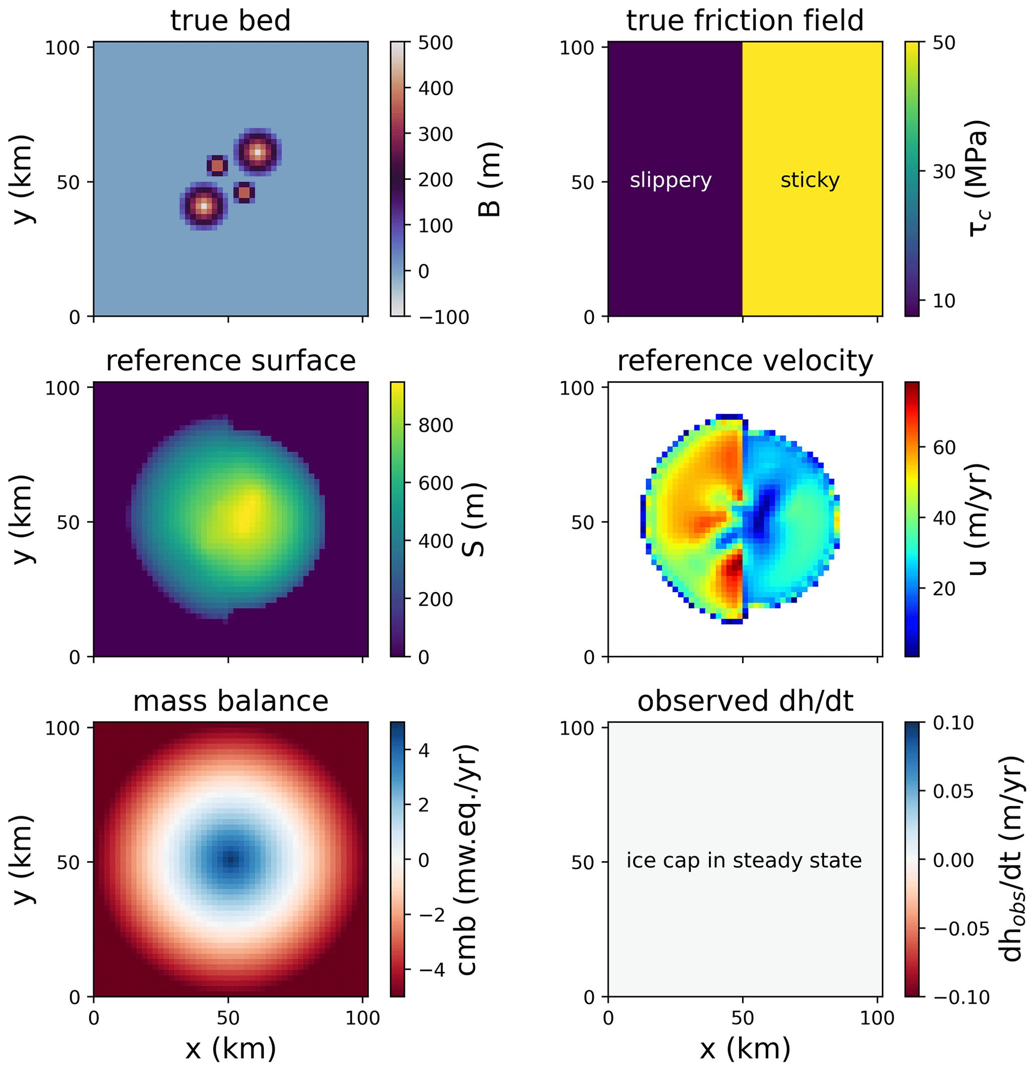
Figure 2 True bed and friction field of the synthetic ice cap, its surface elevation and its velocity after building it and the mass balance and $\mathrm{d}h/\mathrm{d}t$ fields. The latter is zero due to the ice cap being in steady state.

Table 1 Model parameters used for the ice cap and Kronebreen experiments.

After 500 iterations, we apply a friction update according to Eq. (2). Note that this number of iterations between friction updates is rather arbitrary; we choose it here simply because this number is large enough to ensure that the $\mathrm{d}h/\mathrm{d}t$ misfit is sufficiently small at that point so that no more bed updates occur (Fig. 3a). While $\stackrel{\mathrm{‾}}{\left|\mathrm{\Delta }B\right|}$ is generally reduced as the iterative inversion progresses (Fig. 3b), each friction update induces a short response in the ice dynamics that briefly increases $\left|\mathrm{\Delta }\mathrm{d}h\right|$. As seen in Fig. 3b, the steep decline in the bed misfit in these instances demonstrates that those friction updates are crucial for finding the correct bed. The velocity misfit $\left|\mathrm{\Delta }u\right|$ is already close to zero after a few friction updates (Fig. 3c), highlighting that friction changes have a near-instantaneous effect on ice flow speed. A cross section through the ice cap (Fig. 3d) reveals that the bed in the right (sticky) half of the domain is already correctly identified before the first friction update. In the left (slippery) half where the initial friction field does not allow any sliding, however, ice thickness is greatly overestimated at first. This is because, in the absence of sliding, the ice thickness needs to be much greater to be able to achieve an ice flux that is in line with $\mathrm{d}h/\mathrm{d}{t}_{\text{obs}}$ and the mass balance. With each friction update, the bed is made more slippery, which increases flow velocities, thins the ice and lifts up the bed until eventually the correct bed is found here as well. After 8000 iterations, no more changes to the bed occur and we stop the inversion. The final bed (Fig. 3e) is in good agreement with the original one (Fig. 2), as is demonstrated by a near-perfect correlation between the true and modelled ice thicknesses (Fig. 3f) with a coefficient of determination r²=0.997.

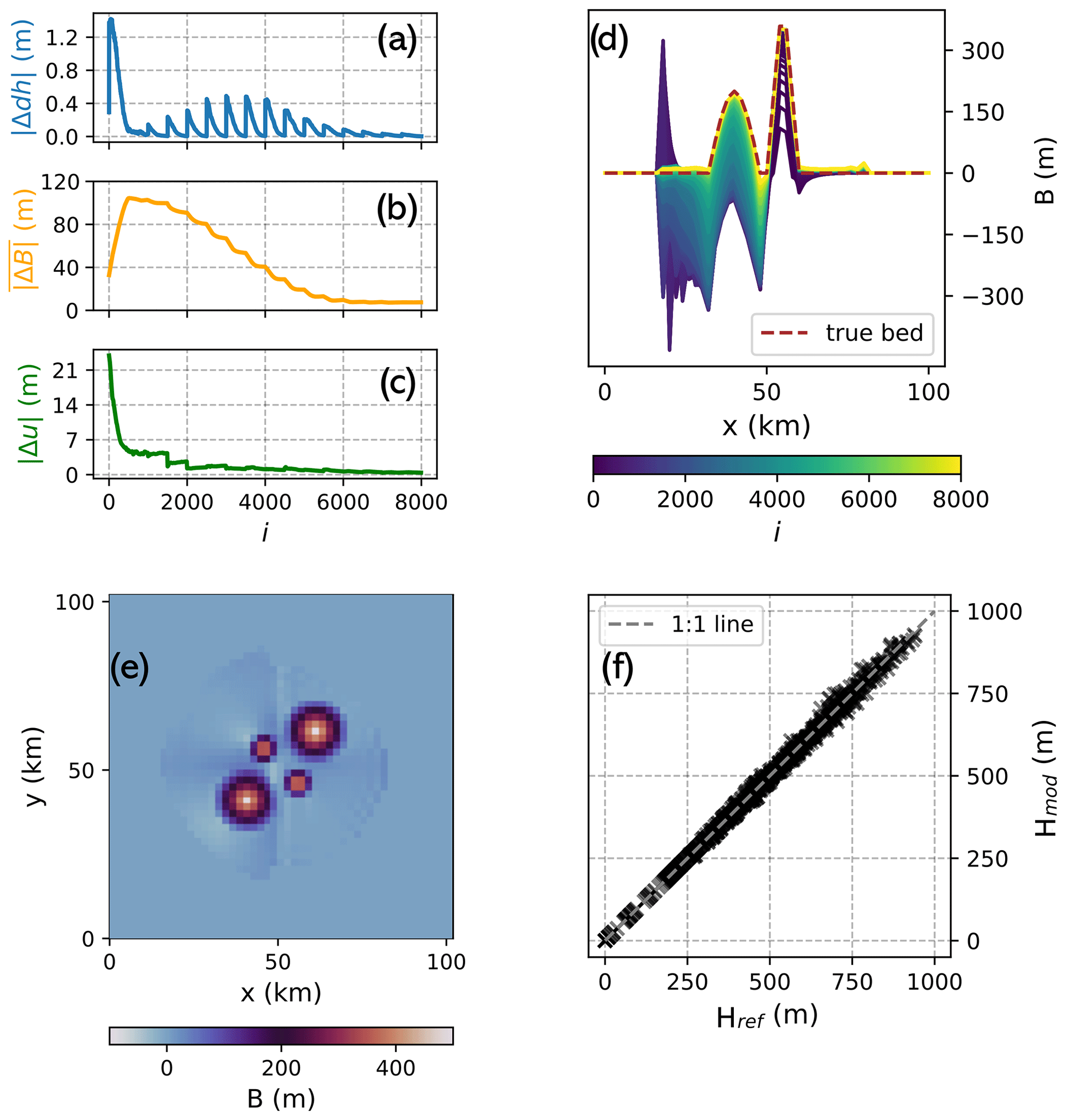
Figure 3 Results of the ice cap inversion. Panels (a–c) show the convergence metrics $\mathrm{d}h/\mathrm{d}t$ misfit (Eq. 5), bed misfit (Eq. 7) and velocity misfit (Eq. 6), respectively, plotted against the iteration number. (d) Cross section through the bed along y=23 km at each iteration step. (e) Final recovered bed. (f) Correlation between modelled and true ice thickness.

To test whether the ice cap setup with the inferred bed and friction field is in a self-consistent steady state after the inversion, we run the model forward in time for 100 years. The ice volume change over this period is 0.18 %, suggesting that this is the case.

3.2 Ice cap sensitivity

Next, we explore how sensitive the inversion is to errors in the input data and to modelling choices. To that end, we use the synthetic ice cap, where we have full knowledge of the “true” parameters. In the following, we provide an overview of the results, while detailed figures and more elaborations can be found in the Appendix.

3.2.1 Input errors

We test the sensitivity to changes in the input mass balance (which is equal to modifying $\mathrm{d}h/\mathrm{d}t$, since it can be shown that those two parameters may be understood as one through the concept of the apparent mass balance, Farinotti et al., 2009) and velocity in experiments where their magnitude is reduced or increased by 25 %, 50 % and 75 %, respectively, relative to their true value at each point in the domain. Furthermore, we conduct experiments where we introduce random surface elevation noise with standard deviations of 5, 10, 15 and 25 m. Finally, we modify the ice temperature from its true value of 268 K to values of 264, 266, 270 and 272 K. For the sensitivity tests of mass balance and ice temperature, we investigate two scenarios: in one, we assume that the true friction field is known, and hence no friction updates are applied; in the other, we assume no prior knowledge of the friction field, requiring inversion for this parameter. Statistics on the ice cap volume error and the final bed misfit $\stackrel{\mathrm{‾}}{\left|\mathrm{\Delta }B\right|}$ (Eq. 7) are shown in Table 2.

Table 2 Sensitivity of the ice cap to input errors in the mass balance, velocity, surface shape and ice temperature. In each table cell, the upper number indicates the magnitude of the perturbation, the lower-left number the ratio between the modelled ice volume given the perturbation and the true ice volume ($\frac{V}{V_{\text{true}}}$), and the lower-right number the final bed misfit $\stackrel{\mathrm{‾}}{\left|\mathrm{\Delta }B\right|}$ (Eq. 7). Results are shown for a scenario with an unknown friction field, i.e. where friction updates according to Eq. (2) are executed, and a scenario where the true friction field is prescribed from the start.

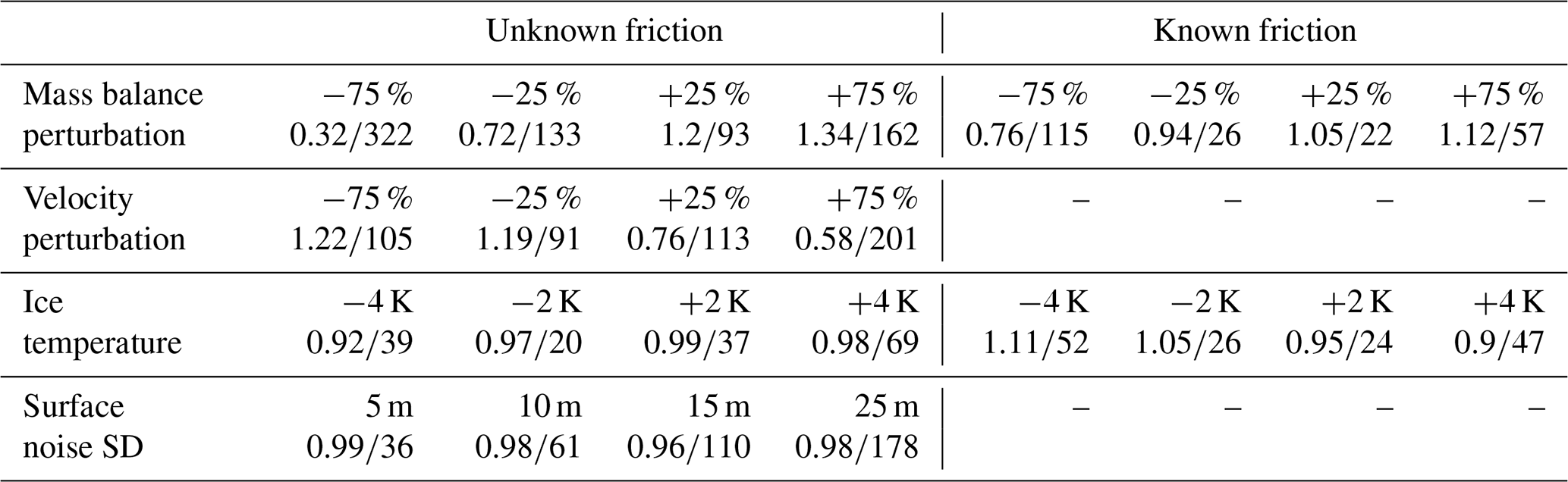
With a known friction field, mass balance errors translate into ice volume errors as the fifth root, as is expected from the theory for shear-dominated flow (Cuffey and Paterson, 2010). This implies that, without friction updates, the method is quite insensitive to errors in mass balance. For example, a 75 % mass balance overestimation results in only a 12 % volume error (Table 2). With friction updates, however, mass balance (and $\mathrm{d}h/\mathrm{d}t$) errors are reinforced. Consider, for instance, a negative mass balance error: this yields overall smaller ice thicknesses and therefore reduced driving stresses, which in turn results in slower ice flow. To match the observed velocities, sliding must be increased when friction updates (Eq. 2) are applied, resulting in further thinning of the ice. Consequently, a 75 % mass balance underestimation leads to a 68 % volume error. The same effect but with the opposite sign follows from a positive mass balance error.

Errors in the observed ice velocity lead to mechanistically similar outcomes. A negative error here means that the bed is made stickier than it should be, resulting in too-thick ice. However, this overestimation of ice thickness induces too-large ice-deformational velocities, leading to an even stickier bed when Eq. (2) is applied, thus causing further thickening. Again, the opposite is the case for a positive velocity error. For the ice cap, a −75 % velocity error results in an entirely non-sliding ice cap with an overestimation of ice volume by 22 %, while a +75 % velocity error leads to a 42 % ice volume underestimation (Table 2).

In the case of ice temperature errors, friction updates have a compensating effect. For instance, a positive ice temperature error causes less-stiff ice and hence too-fast flow, which leads to too-thin ice without friction updates (10 % ice volume underestimation for a +4 K ice temperature error). With friction updates, however, too-fast flow results in a positive velocity mismatch (Eq. 2) leading to a stickier bed, which, in turn, thickens the ice again (2 % volume underestimation for +4 K error).

For surface noise, we find that it changes the bed shape, with already small surface perturbations causing large bed responses (Fig. 4), as is expected from theory (Raymond and Gudmundsson, 2005; Bahr et al., 2014). For instance, surface noise with a standard deviation of 5 m results in $\stackrel{\mathrm{‾}}{\left|\mathrm{\Delta }B\right|}=\mathrm{36}$ m (Table 2) compared to $\stackrel{\mathrm{‾}}{\left|\mathrm{\Delta }B\right|}=\mathrm{7}$ m in the unperturbed experiment. Increasing the regularization parameter θ serves to mitigate these issues (Sect. 3.2.2; Fig. 4). Regardless of the magnitude of surface noise, we find that the calculated final ice volume is largely unbiased (only 2 % volume error even with 25 m surface noise).

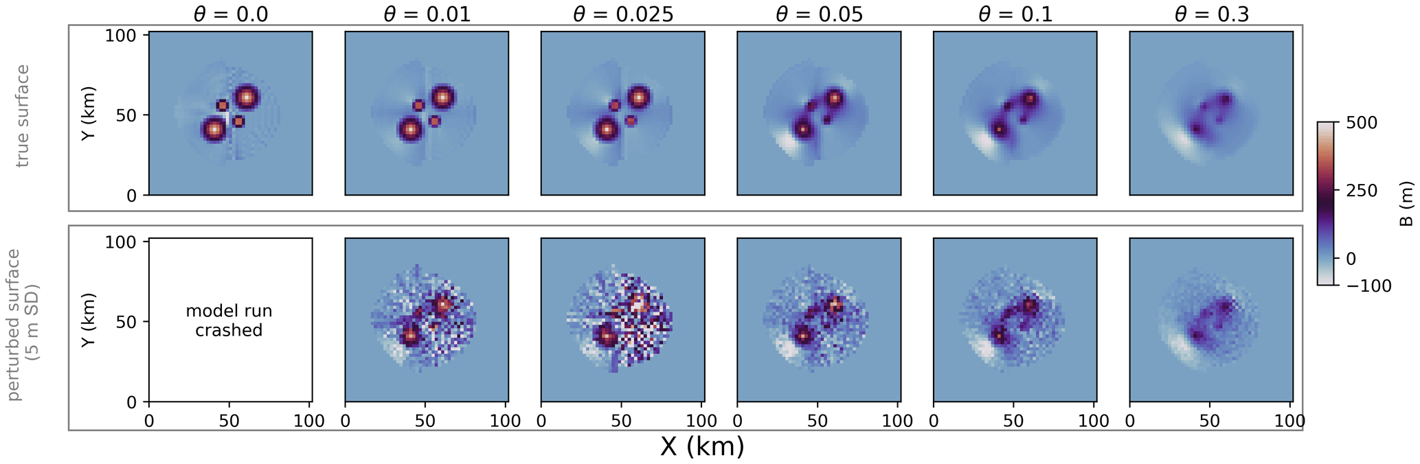
Figure 4 Final bed shape as a function of changing the regularization parameter θ. Upper row: setup without a perturbed surface. Lower row: surface perturbed by adding random noise with a standard deviation of 5 m.

Overall, the exact magnitude of how errors in the input translate into bed and volume errors as well as the strength of amplifying or damping effects of friction updates depend on several characteristics that vary between glaciers, e.g. sliding magnitude and extent. The results obtained here for the ice cap can therefore serve as a baseline estimate for error magnitudes but cannot be directly generalized to other settings.

3.2.2 Inversion parameters

We now investigate how different parameter choices for the inversion influence results. Specifically, we investigate the length dt of the ice flow model forward simulation (the tested values are 0.01, 0.025, 0.05, 0.25, 0.5 and 1 year), the relaxation parameter β (Eq. 1; 0.25, 0.5, 0.75, 1.25, 1.75, 2, 3, 5), the regularization parameter θ (Eq. 3; 0, 0.01, 0.05, 0.1, 0.3) and the role of initial conditions.

We find that our results show virtually no dependence on dt. Likewise, the recovered bed and friction field are not sensitive to their initial guess. For β, larger values lead to faster convergence but lower detail in the recovered bed as compared to smaller values. This is because a large β can cause the bed to oscillate around its true value. The largest influence on the recovered bed is θ, which serves to balance observations and model physics in the presence of input errors as well as to regularize the solution. Larger expected errors in input data require a larger θ to allow the model to accommodate these “unreproducible” characteristics of the data. However, this increases the dependence on initial conditions and loss of detail in the modelled bed since it means that parts of the non-erroneous observations are also accommodated by surface updates rather than bed adjustments (Fig. 4). Regardless of the quality of the input, we find that choosing θ>0 is beneficial for avoiding small bed irregularities in the solution that are not justified by the input data.

4 Application to Kronebreen

Next, we apply our method to the tidewater glacier Kronebreen on Svalbard (Fig. 5). By Kronebreen we refer here to a combined glacier system consisting of the ice cap Holtedahlfonna feeding the outlet glacier Kronebreen. The glacier system covers an area of ∼380 km² and an elevation range from sea level to around 1400 m. The highest flow velocities of up to >1000 m a⁻¹ are found on the highly crevassed glacier tongue (Schellenberger et al., 2015). Due to the large availability of in situ and remote-sensing data, Kronebreen has in recent years been the subject of numerous glaciological studies on ice dynamics (e.g. Schellenberger et al., 2015; Vallot et al., 2017), mass balance (e.g. van Pelt and Kohler, 2015; Deschamps-Berger et al., 2019), sub-glacial hydrology (How et al., 2017), calving (Luckman et al., 2015; Vallot et al., 2018), perennial firn aquifers (Christianson et al., 2015), seismicity (Köhler et al., 2019) and basal topography (Lindbäck et al., 2018a).

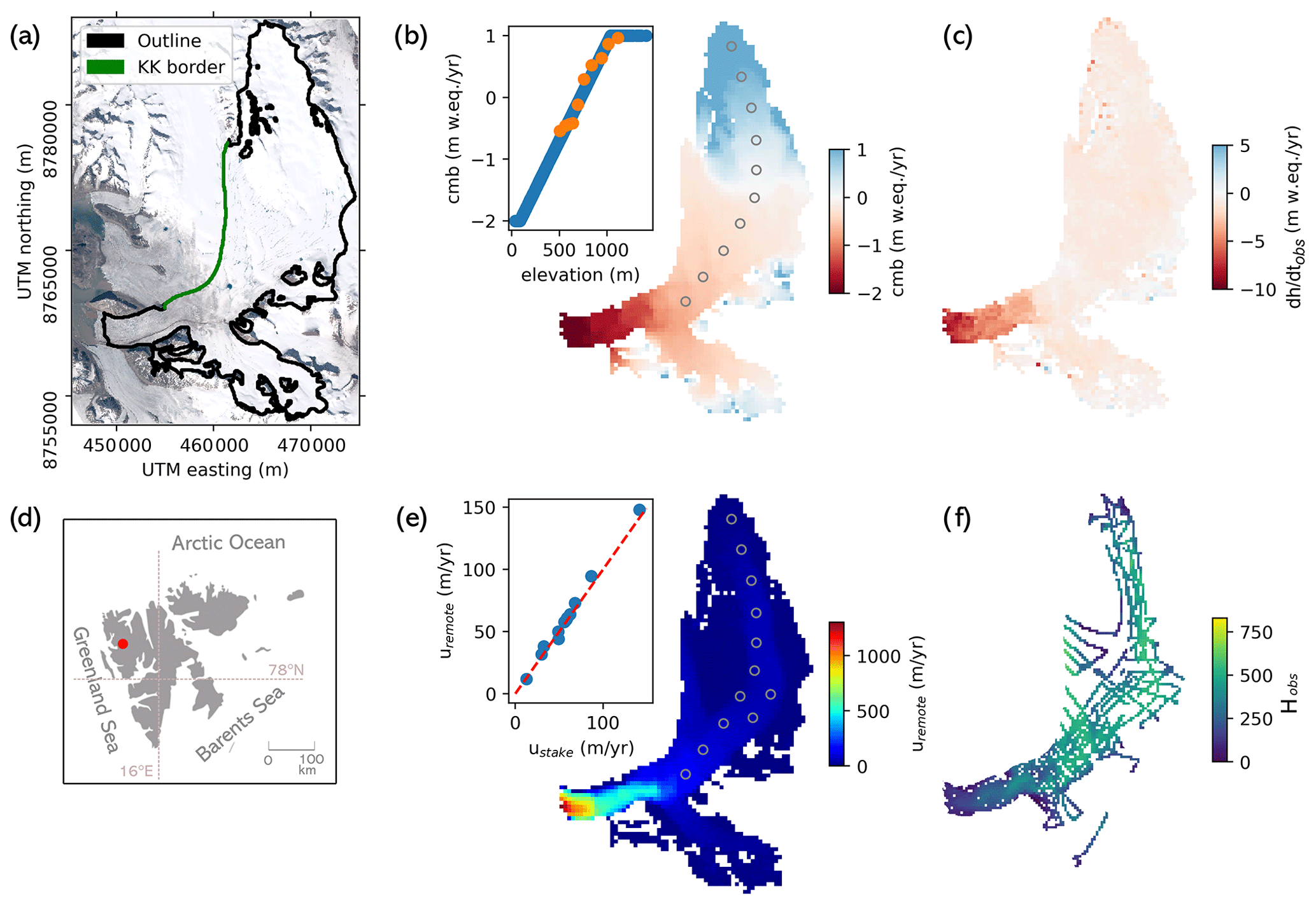
Figure 5 Input data for Kronebreen inversion (the coordinate system is UTM zone 33N). (a) Kronebreen outline in black and border to the neighbouring glacier Kongsbreen (KK border) in green. (b) Climatic mass balance derived from extrapolating stake observations (locations shown by circles in the main plot and values by orange dots in the inset) to the entire glacier using an elevation-dependent linear model (inset plot). (c) Observed rate of surface elevation change $\mathrm{d}h/\mathrm{d}t$ as computed by subtracting two digital elevation models. (d) Location of Kronebreen in Svalbard (marked by a red dot). (e) Observed velocities from remote sensing (Millan et al., 2022a) validated with stake observations (inset plot). (f) Radar observations of ice thickness (Lindbäck et al., 2018a).

4.1 Observational data

The input data for the thickness inversion of Kronebreen comprise two DEMs based on Pléiades imagery from 2014 (Deschamps-Berger et al., 2019) and 2020, which we use to generate a $\mathrm{d}h/\mathrm{d}t$ field $\frac{\mathrm{d}{h}_{\text{obs}}}{\mathrm{d}t}=\frac{S_{\mathrm{2020}}-S_{\mathrm{2014}}}{\mathrm{6}}$ (Fig. 5). The 2020 DEM has some holes at higher elevations in the southern part of Kronebreen that we fill using 2014 data. Since $\mathrm{d}h/\mathrm{d}t$ would hence be zero there, we generate a $\mathrm{d}h/\mathrm{d}t$ field as a function of surface elevation, which we use to patch those holes. Whether to use the 2014 DEM, the 2020 DEM or a mean of the two as the input surface for the ice dynamics model is not an obvious choice. From a theoretical point of view, the surface that gave rise to (or was the product of) the aggregate ice dynamics in the period 2014–2020 should be used. While this would favour using the mean of the two DEMs, it would imply using a surface that may not ever have existed. We therefore choose to use the 2020 DEM instead as this avoids complications at the terminus where Kronebreen has retreated. There, differencing or taking a mean of the two DEMs would not yield a representative $\mathrm{d}h/\mathrm{d}t$ field or glacier surface because the difference and the mean between the 2014 surface elevation and sea level (which is what the 2020 DEM shows) do not reflect the true ice loss or a realistic glacier surface shape. In terms of mass balance, we use observations from 10 stakes placed approximately along the central flow line of Kronebreen and covering an altitude range from 505 m (mean over 2014–2020: −0.53 $\mathrm{m}\mathrm{w}.\mathrm{e}.{\mathrm{yr}}^{-\mathrm{1}}$) to 1116 m (mean: 0.96 $\mathrm{m}\mathrm{w}.\mathrm{e}.{\mathrm{yr}}^{-\mathrm{1}}$) to generate a linear mass balance gradient, which we apply over the whole altitudinal range of Kronebreen (Fig. 5b). Following general observations made at glaciers in Svalbard, we cap the maximum mass balance at 1 m yr⁻¹ (similar to van Pelt and Kohler, 2015). Internal and basal mass balances are neglected. Finally, we use surface velocity observations from Millan et al. (2022a) with a nominal date of 2017–2018 (Fig. 5e). Their performance is validated using measured stake velocities (mean difference: 2.4 m yr⁻¹ / 3.5 %).

For validation of the modelled thicknesses, we use an extensive data set of measured bed elevations acquired using ground-penetrating radar (Lindbäck et al., 2018a, Fig. 5f). The errors associated with those data are of the order of 10 m where the ice is thin (mainly along the fast-flowing lower reaches of Kronebreen) and up to 30 m in the upper thick parts of Kronebreen. We resample the radar tracks to a grid of 400 m resolution to match it with the model results.

4.2 Modelling choices

We set up a rectangular modelling domain with a regular grid spacing of 400 m. We define a glacier mask based on manually drawn outlines of Kronebreen using satellite imagery and ice flow observations. Inside the mask, we allow ice to exist, while in all other parts of the domain, the ice thickness is forced to zero by resetting the bed height to the surface height. The mask also covers some small parts of what is believed to belong to the neighbouring glacier Kongsbreen, where we have a surface DEM from 2020. Since the boundary between Kronebreen and Kongsbreen is not perfectly known, some ice exchange here cannot be excluded. While our experiments indicate that this is a better approach than cutting the mask at the assumed Kronebreen–Kongsbreen border (not shown), some boundary effects can still not be ruled out since we only model a small part of Kongsbreen, thus not accounting for the entire mass flux potentially reaching the Kronebreen–Kongsbreen border in reality. At all the other mask boundaries, we do not apply any flux constraints or lateral friction since the friction inversion will account for lateral drag if needed.

At the glacier terminus, we apply the hydrostatic water pressure. We also remove all floating ice and do not allow calving; this is because we cut off all ice outside the mask after each iteration anyway, hence artificially “calving” all ice that has advanced beyond the known glacier extent. Furthermore, we need to ensure that, in each forward simulation, the ice can advance into the ocean unblocked by the bathymetry in front of the glacier (which is unknown). We therefore apply a zero bed slope in the flow direction at the ice–ocean boundary.

Ice flow is described by the SSA + SIA hybrid scheme available in PISM (Bueler and Brown, 2009). Note that, while the SSA accounts for membrane stresses, the SIA does not, and so ice flows strictly downhill in the absence of sliding (see Sect. 4.5). Furthermore, we set an isothermal flow law with a fixed ice temperature of 0 ^∘C (Table 1), where the ice softness A is $\mathrm{3.96}\times {\mathrm{10}}^{-\mathrm{24}}{\mathrm{s}}^{-\mathrm{1}}{\mathrm{Pa}}^{-\mathrm{3}}$. This assumption follows from observations and modelling at many Svalbard glaciers where extensive meltwater refreezing in the firn keeps the ice close to the melting point (e.g. van Pelt et al., 2019). In the bare ice areas of the ablation zone and near the glacier edges, the largest deviations from this assumption can be expected. We choose a linear sliding law by setting the parameters q=1 and u_th=1 m s⁻¹ in Eq. (8). This causes the sliding velocity to be directly proportional to the velocity misfit (Eq. 2), thus stabilizing the inversion.

4.3 Initial conditions

We derive an initial bed guess by subtracting, from the input 2020 DEM, an initial ice thickness H_init calculated with the perfect plasticity assumption (Nye, 1952), such that

$$\begin{array}{}\text{(9)}& H_{\text{init}}={\displaystyle \frac{{\mathit{\tau }}_{\mathrm{b}}}{\mathit{\rho }g\sin \mathit{\alpha }}},\end{array}$$

where ρ is the ice density, g is gravitational acceleration, α is the surface slope as computed from the input DEM and τ_b is the basal shear stress that we arbitrarily set to τ_b=120 kPa. Based on the sensitivity experiments with the artificial ice cap, we do not expect the choice of τ_b to impact our results significantly. We iteratively smooth the derived thickness field over 4 times the ice thickness to account for longitudinal stress gradients (Kamb and Echelmeyer, 1986), and we apply a Gaussian kernel to remove small-scale variability not justified by the input data (Habermann et al., 2012).

For basal friction, we derive an initial guess of τ_c in Eq. (8) as ${\mathit{\tau }}_{\mathrm{c}}=\frac{{\mathit{\tau }}_{\mathrm{d}}{u}_{\text{th}}}{u_{\text{obs}}}$, where τ_d is the driving stress at the start of the inversion calculated as τ_d=ρgH_inittan α (Vallot et al., 2017).

4.4 Inversion parameters

We set the forward-modelling time step dt to 0.01 years (Table 1). This small value allows a fast inversion, while our experiments show that the results are not sensitive to this choice. From the stabilization techniques (Sect. 2.3) we only apply the β ramp-up (with i_s = 10 and β₀=0.5) and input data smoothing to the DEM. Since we assume that we have high-quality input data, we apply only weak regularization by setting the parameter θ=0.05, meaning that 5 % of bed updates are changing the surface in the opposite direction. Based on our experiments, we see that, after ∼8000 iterations, no more changes to the bed or friction field occur, and so we stop the inversion there. We also see that it takes at most ∼1000 iterations after a friction update to converge to a solution, making this our interval for updates of τ_c (Eq. 2).

4.5 Kronebreen inversion results

We find that the iterations consistently reduce the $\mathrm{d}h/\mathrm{d}t$ misfit (Eq. 5) interrupted by friction updates, as expected (Fig. 6d). Owing to the surface updates, the misfit approaches zero in each interval between friction updates, showing that, with our regularization method, no stopping criterion is needed. The bed and velocity misfits are equally reduced with each iteration. It turns out that our initial bed guess overestimated ice thickness in most parts of the domain as the bed generally becomes shallower. This is particularly true at the fast-flowing outlet glacier, where the friction updates decrease basal drag and thus are instrumental in ensuring that ice thickness there is not overestimated. The final mismatch between modelled and observed velocity magnitudes is generally of the order of a few percent where the glacier is sliding, while it is above 50 % in some of the non-sliding parts of the accumulation area (Fig. 6a). Overall, this indicates that the friction updates have helped to align model dynamics with reality.

Figure 6 Raw output of Kronebreen inversion. (a) Velocity misfit with purple colour indicating where modelled velocities exceed observed velocities by more than 50 %. (b) Difference between radar-derived and modelled bed elevation. (c) Zoom into the area with the largest bed deviations for observed velocities, modelled velocities and surface aspect (with arrows denoting the downhill direction and colours showing into which sector the ice surface is sloping). (d) $\mathrm{d}h/\mathrm{d}t$ (Eq. 5), bed (Eq. 7) and velocity misfit (Eq. 6) per iteration.

When comparing with observed bed elevations from radar measurements, we see that our ice thickness generally matches the observations well, with deviations of the order of a few tens of metres (Fig. 6b). However, there is one larger area where our ice thickness is greatly overestimated by more than 250 m. This area is a flat and slowly flowing part which, as shown by the observed flow velocities, is only weakly connected to the main flow and hence only receives little ice from upstream (Fig. 6c). However, in our model, there is a distinct “flow channel” diverging from the main flow through which ice is discharged into that area. Where the flow channel diverges in the model, basal velocities are close to zero, meaning that internal shear controls ice flux. As mentioned before, in the absence of sliding, the shear-dominated flow calculated by the SIA is strictly downhill. Indeed, the input DEM is sloping towards the flow channel in that area (Fig. 6c). We hence conclude that, in reality, there are likely membrane stresses forcing the ice to not flow downhill that are not resolved by the model physics, thus causing a mismatch in flow directions. Because of this, the ice flow model discharges ice into a slow and flat area where, as is known from theory (Gudmundsson, 2003; Raymond and Gudmundsson, 2005), errors in the flux will lead to large errors in the bed. Note that friction updates are of no help here: since the ice is too thick in the area, ice velocities in the model are larger than in reality due to enhanced internal deformation, which means that a friction update makes the bed stickier (even if there already is no sliding), while the opposite would be needed to lift up the bed. Reflecting the large ice thickness overestimation in a small part of the domain and, consequently, a skewed distribution of the differences between modelled and observed bed heights, the final mean absolute bed misfit is $\stackrel{\mathrm{‾}}{\left|\mathrm{\Delta }B\right|}=\mathrm{108}$ m, while the median absolute bed misfit is 66 m.

4.6 Kronebreen post-processing

To improve the results of the inversion, an optional post-processing step can be applied. While this brings the modelled bed closer to observations, it conflicts with the consistency between model physics, input observations and the bed, resulting in similar problems for ensuing prognostic simulations as encountered with many other thickness inversion methods (Sect. 1).

In the post-processing, we use the velocity observations to identify areas that are likely too thick. Specifically, we scan the model domain for areas where the ice velocity through internal deformation exceeds the observed velocities. Assuming that the ice viscosity estimate is correct, a too-large ice thickness is the only first-order control on ice dynamics not constrained by the inputs that could induce higher velocities than observed in the absence of basal sliding. We apply this logic and conservatively only mark areas where the observed ice velocity is exceeded by at least 50 % to account for errors in the velocity observations (purple areas in Fig. 6a). Indeed, this reliably identifies the area where the mismatch in flow directions induces the largest errors in the modelled bed and picks out other locations where the ice thickness is overestimated (as shown by the radar validation). To update the bed elevation estimate in this area, we turn towards an analytical ice thickness equation based on the SIA (e.g. Millan et al., 2022a) in which ice thickness H can be inferred from observed velocities such that

$$\begin{array}{}\text{(10)}& H={\left({\displaystyle \frac{(u_{\mathrm{s}+}-u_{\mathrm{b}})(n+\mathrm{1})}{\mathrm{2}A(\mathit{\rho }g\mathit{\alpha }{)}^n}}\right)}^{\frac{\mathrm{1}}{n+\mathrm{1}}},\end{array}$$

with n=3 being Glen's flow law exponent (Glen, 1955) and u_s and u_b being the surface and basal velocities, respectively. Note that this equation requires a minimum slope α_min, which we set to 0.025 (e.g. van Pelt et al., 2013) to prevent ice thickness from going to infinity as α approaches zero. Furthermore, note that u_s+ refers here to u_s+0.5u_s to account for the uncertainty in velocities. With this post-processing step, we are able to greatly reduce the errors in the modelled bed. After smoothing the computed bed with a Gaussian kernel, we arrive at a mean absolute deviation from observations (Eq. 7) of 78 m and a median absolute deviation of 55 m (Fig. 7).

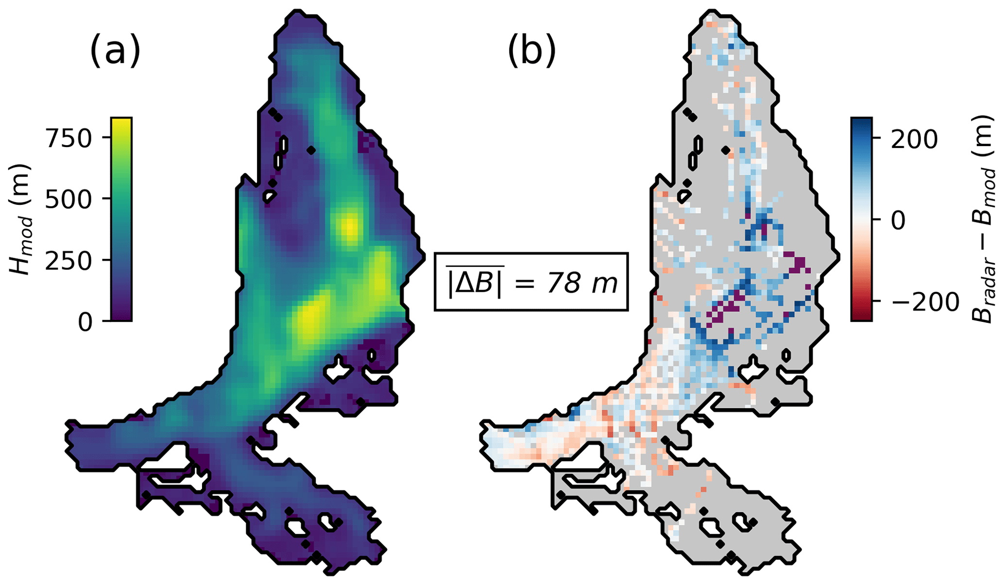
Figure 7 Final output after “post-processing”. (a) Modelled ice thickness. (b) Bed elevation error as compared to radar observations, with a mean absolute error (Eq. 7) of 78 m.

4.7 Kronebreen sensitivity to mass balance

From the input data sets, the least constrained one is arguably surface mass balance, since we rely on a few stakes that are extrapolated to the entire glacier. An ice core drilled in 2005 on an ice divide in the upper accumulation area (1200 m a.s.l.) of Kronebreen indeed shows considerably lower accumulation (0.5 $\mathrm{m}\mathrm{w}.\mathrm{e}.{\mathrm{yr}}^{-\mathrm{1}}$ during 1963–2005, van der Wel et al., 2011) than the values we use here (1 $\mathrm{m}\mathrm{w}.\mathrm{e}.{\mathrm{yr}}^{-\mathrm{1}}$), demonstrating that there is large spatial inhomogeneity likely as a result of variability in wind exposure and the associated snow redistribution. This is also known from other Svalbard glaciers (e.g. van Pelt et al., 2014). The velocity misfit map of our raw output indicates that in large parts in the accumulation area the ice is flowing too quickly despite no or very limited basal sliding (Fig. 6a). While this could also be the result of a too-high ice viscosity (note, however, that we already use an ice temperature of 0 ^∘C), a likely explanation is a too-positive mass balance that induces too-thick ice and hence too-fast surface motion by internal deformation. We therefore repeat our thickness inversion after multiplying the mass balance by 0.8. Indeed, this yields a better result with a mean absolute deviation of 100 m (and a median absolute deviation of 61 m) before post-processing. The velocity misfit in the accumulation area is also reduced.

5 ITMIX synthetic glaciers

To benchmark our method against other ice thickness inversion approaches, we finally test it on three glaciers from the ITMIX intercomparison study (Farinotti et al., 2017, 2021). The experiments are performed in the style of the first ITMIX, i.e. without using any thickness observations during the inversion (Farinotti et al., 2017). For general details on the setup of the intercomparison study, the reader is referred to the publications referenced above. Due to the necessity of having consistent input data and the unsuitability of applying PISM to real-world mountain glaciers (Sect. 6.5), we are limited to the three synthetic glaciers within ITMIX, i.e. glaciers that were artificially grown using a higher-order ice dynamics model and a prescribed mass balance field over smoothed real-world deglacierized topographies. They represent a valley glacier, a mountain glacier and an ice cap, respectively. The provided input fields comprise surface topography, climatic mass balance, $\mathrm{d}h/\mathrm{d}t$ and ice flow velocities.

For the inversion, we this time assume no sliding, which hence means relying on the SIA alone. Instead of applying friction updates, we use the provided ice flow velocities to constrain the otherwise unknown ice temperature in an analogous way; i.e. we update an initial guess of glacier-wide ice temperature (270 K) based on the mismatch between median modelled and “observed” ice speed. This is done every 500 iterations, while the total number of iterations is set to 2500. From the stabilization techniques, we only apply ice margin interpolation. The inversion parameters are set to dt=0.1 years, β=0.3 and θ=0.1. To derive a first guess of ice thickness, we rely on the perfect-plasticity method (Nye, 1952, Eq. 9), where we estimate the basal shear stress using an established relationship with the glacier altitudinal range as described in Haeberli and Hoelzle (1995). In terms of post-processing, we only fill holes in the ice thickness field by interpolation and apply a Gaussian filter to the solution.

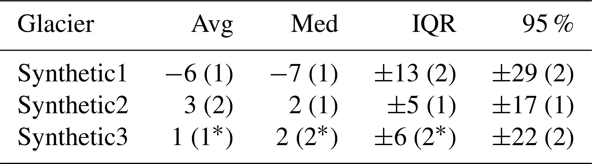
We find excellent agreement with the thickness “observations” provided (Table 3, Figs. A7–A9). The average deviation, indicative of volume biases, is generally low, as are the interquartile range and the 95 % confidence intervals, suggesting that the bed shape is well represented. With the performance indicators used by ITMIX, our results are always either best or second best among all the solutions submitted to ITMIX.

Table 3 Following ITMIX1, the average (Avg), median (Med), interquartile range (IQR), and 95 % confidence interval (95 %) of the deviations from ice thickness measurements are given for the three glaciers as percentage deviations from the mean ice thickness. The numbers in parentheses are the rank of every value relative to all other solutions submitted to ITMIX1 (Farinotti et al., 2017). ^* indicates shared ranks.

6 Discussion

We presented here a new thickness inversion method and tested it on a synthetic ice cap, the tidewater glacier Kronebreen in Svalbard and three ITMIX glaciers. It reconciles bed topography and ice dynamics because it produces ice thickness and basal friction fields that are consistent between the dynamic state of a given glacier, input observations and the ice flow equations as represented in ice dynamics models. It is versatile because it can utilize any complexity of ice physics, from simple SIA approximations to full Stokes models. Together, these two characteristics make it highly suitable for prognostic simulations that should start from a self-consistent glacier state (Goelzer et al., 2017). Finally, it is fast because each iteration step consists of only a short forward simulation, e.g. dt=0.01 years. For our test glacier Kronebreen, we computed 8000 iterations, resulting in a net model time of 80 years, which can be compared to other approaches yielding a similar output that require several thousands (e.g. van Pelt et al., 2013; Le clec'h et al., 2019) to millions of years of model time (e.g. Pollard and DeConto, 2012) or computationally expensive adjoint-based inversions (e.g. Goldberg and Heimbach, 2013).

6.1 Sensitivity experiments

While always converging to a bed solution, the experiments with the synthetic ice cap showed that errors in input data can have varying impacts on the modelled bed depending on the inversion setup. With friction updates, the method is less sensitive to errors in ice temperature than without friction updates, since the modelled basal friction field can compensate for ice viscosity errors. However, the method is more sensitive to errors in mass balance and $\mathrm{d}h/\mathrm{d}t$ with friction updates since an underestimation (overestimation) of mass flux and hence ice thickness reduces (increases) internal deformation, prompting changes in the friction field that further exacerbate the error. Likewise, errors in velocities reinforce themselves. Because of this, we argue that friction updates should be used with caution, i.e. only when it is likely that sliding is important for a specific glacier and when the input data are of a sufficient quality. Indeed, for both the synthetic ice cap and Kronebreen, not doing friction updates would have required us to assume a friction field without any knowledge of whether it is reflective of the true basal conditions or not, hence resulting in a somewhat arbitrary bed shape. For slow-flowing mountain glaciers with only poor velocity observations, however, it may be more meaningful to assume a friction field or simply not allow any sliding. In the case of non-sliding mountain glaciers with high-quality velocity data, we show that velocity observations can be used to tune other unknowns, e.g. the ice temperature. Regarding errors in an input DEM, we showed that our regularization methodology involving small adjustments to the surface in each iteration is capable of producing a reasonable bed shape even in the presence of considerable surface errors, albeit with less spatial detail and stronger dependence on initial conditions for larger values of the regularization parameter θ. Generally, the comparatively large sensitivity of a bed inversion to the input surface is an inherent problem that follows from the ill-posed nature of all thickness inversions and is thus largely unavoidable (Bahr et al., 2014).

6.2 Comparison with other inversion methods

The method performed excellently in the ITMIX experiments, ranking among the best two approaches for all glaciers and performance metrics assessed (Table 3). Although the glaciers tested are synthetic with perfectly known input data, the model physics used in the inversion (SIA) are incomplete as a higher-order model was applied to grow the glaciers (Farinotti et al., 2017), confirming that the method is capable of accommodating such imperfections. The consistently good results speak to the general skill of the approach and its versatility when applying it to different glacier types, and they highlight the method's usefulness for inferring ice thickness, especially when no bed observations are available.

To provide a further perspective, we now also set our Kronebreen results in relation to other existing ice thickness products available for that glacier, i.e. to results from the global studies by Millan et al. (2022a) and Farinotti et al. (2019) as well as the Svalbard-wide study by Fürst et al. (2018). Millan et al. (2022a) mapped global ice flow velocities and computed ice thickness from Eq. (10) while calibrating the ice viscosity region-wide based on observed ice thicknesses. The Farinotti et al. (2019) product is an ensemble of several inversion methods, and for Kronebreen three different model results are available. One is equivalent to Fürst et al. (2018), while the other two are different implementations of a mass conservation approach as described in Huss and Farinotti (2012) and Maussion et al. (2019), respectively. Again, thickness observations were used in these latter two methods to calibrate certain model parameters on a regional or glacier-wide scale. Fürst et al. (2018) is also a mass conservation approach but completely assimilates existing ice thickness observations and thus cannot be validated independently for Kronebreen. We therefore show the bed misfits $\stackrel{\mathrm{‾}}{\left|\mathrm{\Delta }B\right|}$ only for Millan et al. (2022a), Huss and Farinotti (2012) and Maussion et al. (2019) alongside the values obtained in this study with corresponding scatter plots of modelled against observed ice thicknesses in Fig. 8. Before post-processing, our method performs worse than Millan et al. (2022a) but better than the other two approaches. After post-processing, our results have the lowest bed error despite being completely independent of thickness observations, in contrast to all the other studies.

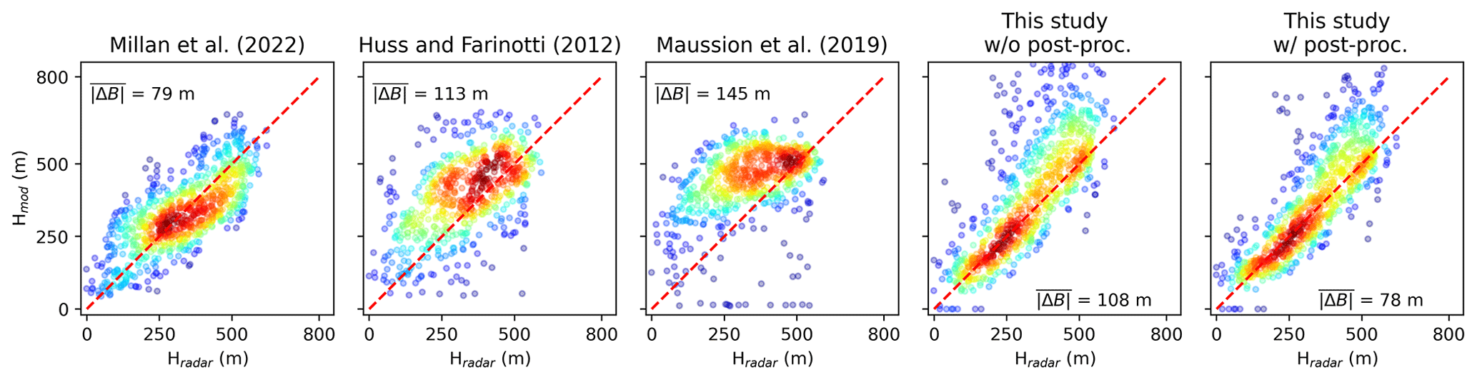
Figure 8 Correlation between radar-derived and modelled ice thicknesses for different ice thickness products available for Kronebreen (colours indicate point density) with the mean absolute difference annotated. The red dashed line is the 1:1 line.

6.3 On internal model consistency

The inversion method presented here places great weight on internal model consistency, meaning that no bed can be computed that is at odds with the ice flow model physics. While this ensures that the output will be in line with all fundamental principles of ice dynamics, it also means that a real-world process that is not reflected in the physics of the forward model will – if not accounted for otherwise – result in errors in the bed shape. As such, unregularized data and model errors are subsumed in the final bed, as seen for the Kronebreen experiments. While it is possible to estimate how errors in the input data are propagated to bed errors, this is unfortunately not true for model errors, which are difficult to quantify. Using our “post-processing” approach as outlined in Sect. 4.5, however, allows alleviation of some of the possible errors. Such an approach represents an interference with model physics in favour of a more accurate bed map and should therefore be applied when the modelled bed likely contains significant errors. This may be assessed based on the mismatch in observed and modelled velocities as shown here. If only minor deviations are found, we propose refraining from any post-processing to conserve the consistency between bed, model physics and input observations.

From the emphasis on internal consistency also follows that providing ice thickness observations and fixing the bed heights where they are available does not help to improve the results, as we find in experiments that are not shown here. When artificially fixing the bed height at a location, an inconsistency is created which the model cannot take advantage of. To assimilate thickness observations, we rather suggest to use them to tune model parameters, e.g. ice viscosity, as is done in other inversion approaches (e.g. Farinotti et al., 2019; Millan et al., 2022a). With such a strategy, errors in input data can be compensated, thus ensuring an overall unbiased total ice volume estimate.

6.4 On unique solutions

In theory, it is conceivable that several combinations between friction and thickness could reproduce the observations of $\mathrm{d}h/\mathrm{d}t$ and velocity, raising the question of whether the solutions obtained with our inversion are unique. To discuss this, we recall that the concept of the apparent mass balance (Farinotti et al., 2009) shows that $\mathrm{d}h/\mathrm{d}t$ and mass balance together determine the total mass that is fluxed through a glacier. This mass may be transported either by a thick but slow glacier or by a thin but fast glacier. By forcing the model to reproduce observed velocities via the friction coefficient, there would only be one ice thickness that matches the mass flux if ice thickness and ice speed were independent of each other. However, since ice thickness also influences ice speed via the driving stress, there is a small realm of overlap between the two regimes, i.e. when observed velocities can be reproduced by a change in either ice thickness or basal friction. Due to the different characteristics of sliding (non-local, vertically uniform velocity profile) and shearing (local, vertically dependent velocity profile) ice physics, we think that it is typically very unlikely that changing thickness or basal friction would lead to the same ice velocity and mass flux and therefore that non-unique solutions are common. The fact that all of our experiments, synthetic and real-world ones, converge to a sensible bed even with different initial conditions corroborates this idea.

Similar to the above, the question could be raised whether the order between friction and bed updates matters and if it could be changed. From our experiments, we see that changes to the friction field have a near-instantaneous effect on ice velocity, which in turn causes a change in ice thickness, but the convergence to a new state is rapid and the radius of affected grid points is small (although not entirely confined to one grid cell due to the non-local nature of the SSA). Bed updates, by contrast, lead to changes in the mass “export” of an affected cell, and thus affect all downstream grid cells, which will also change their mass “export”. Because of that, bed updates are travelling downstream through the entire glacier, implying that it takes much longer to reach a new state after bed updates. In fact, through this concept, it can be understood that the convergence time to a new bed is equivalent to the response time of the glacier to a mass balance perturbation. Given these differences in convergence time of bed vs. friction updates, we conclude that it does not make sense to swap the order between them.

6.5 Outlook

We did not consider thermodynamics in this study but used a constant ice viscosity parameter. This could account for some errors that we see at Kronebreen. For example, a locally stiffer ice body might have resulted in slightly different modelled flow directions in those places where we find the largest errors. How to implement thermodynamics in our inversion methodology should hence be explored in future work.

Given the low computational cost of the inversion, an application on a large scale could be undertaken. For all the input data sets ready-to-use products already exist on a global scale ($\mathrm{d}h/\mathrm{d}{t}_{\text{obs}}$ by Hugonnet et al., 2021, surface velocities by e.g. Millan et al., 2022a, DEMs from e.g. NASA JPL, 2020, glacier outlines from RGI Consortium, 2017, mass balance by Rounce et al., 2023). However, since mountain glaciers are often poorly represented by shallow ice physics, using PISM may lead to poor results. Instead, a possible solution could be to use the fast ice flow model emulator IGM (Jouvet, 2022), which is a convolutional neural network trained on a full Stokes model.

7 Conclusions

In this study, we have presented a novel thickness inversion approach that combines satellite products and advanced ice flow models to generate distributed maps of sub-glacial topography that are consistent with the dynamic state of a given glacier. The general functional principle is derived from the idea that, among all inputs typically used in ice flow modelling, bed observations are often the least constrained, allowing us to consider that differences between observed and modelled ice dynamics (as represented by $\mathrm{d}h/\mathrm{d}t$) primarily originate from errors in the assumed bed shape. To eliminate this discrepancy, the bed is adjusted iteratively until modelled and observed dynamics are in line. A similar logic is applied to also derive the sub-glacial friction field based on the mismatch between modelled and observed ice flow velocities. We have tested the model on an artificial ice cap (also under a range of perturbations), the glacier Kronebreen on Svalbard and three ITMIX glaciers, where we find excellent performance resulting in a top ranking among all the solutions originally submitted to ITMIX. Since the method is computationally inexpensive and does not require bed observations as input, future applications could include both detailed inversions on the local scale as well as large-scale studies. Furthermore, due to the self-consistent glacier state achieved after the inversion, the method is well suited for initializing prognostic simulations.

Appendix A

Below, we elaborate further and present figures on the sensitivity experiments described in Sect. 3.2.

A1 Input errors

We start by perturbing the mass balance such that it is reduced and increased uniformly in the domain by 25 %, 50 % and 75 %. Mass balance and $\mathrm{d}h/\mathrm{d}t$ jointly control the mass flux through the glacier (and can even be lumped together into one variable following the concept of the apparent mass balance; Farinotti et al., 2009), and so errors in either of them have the same effect. Therefore, we do not investigate them separately here but focus on mass balance alone. A reduction in flux should lead to a thinner glacier and a shallower bed, while the opposite should be the case for an increase in flux, as observed in our experiments (Fig. A1). From the integrated form of Glen's flow law (Cuffey and Paterson, 2010) for shear-dominated flow,

$$\begin{array}{}\text{(A1)}& H=\sqrt[n+\mathrm{2}]{{\displaystyle \frac{q}{\mathrm{2}A}}\cdot {\displaystyle \frac{n+\mathrm{2}}{{\left(\mathit{\rho }g\sin \mathit{\alpha }\right)}^n}}},\end{array}$$

it can be seen that flux (denoted by q) errors translate into thickness errors as the fifth root. If we prescribe the true friction field at the start of the inversion and do not apply any updates to it, the computed ice volumes using the perturbed mass balances follow this relationship accurately. However, with friction updates, there are positive feedback effects that induce larger errors. Since a reduction in mass flux means that the calculated ice thickness is smaller than its true value, the driving stresses are smaller, resulting in slower ice flow. To match the observed velocities, sliding must hence be increased when friction updates (Eq. 2) are applied, resulting in a further thinning of the ice through the associated bed uplift. Therefore, with friction updates, the final ice volume is smaller than what might be expected from the mass balance underestimation alone. The opposite is the case when the mass flux through the glacier is overestimated. In this case, the overestimated ice thickness induces larger driving stresses and hence an overestimation in surface velocities, prompting the friction field to be made stickier during a friction update. This induces further bed lowering, resulting in a stronger overestimation of ice thickness at the end of the inversion. This effect, however, is only present in those areas where the glacier is sliding. In non-sliding areas, a further increase in the friction field will not lead to a thickness increase, putting an upper bound on this positive feedback effect. Quantifying the effects of flux errors when friction updates are applied is, therefore, more difficult than when no friction updates are applied. Both the ratio between sliding and non-sliding areas in the glacier and the sliding magnitude control the final errors. Generally though, due to the above, an underestimation of ice flux introduces larger errors than an overestimation, and so we find that, for our artificial ice cap, negative mass balance errors translate about linearly into volume errors, while positive ones introduce errors to a power somewhat below one (Fig. A1).

Figure A1 (a) Modelled ice volume after the inversion relative to the true ice volume of the ice cap as a function of mass balance perturbations. Colours indicate the mean absolute deviation between the inverted bed and the true bed. Triangles represent runs where the true friction field was prescribed from the start of the inversion, meaning that no friction updates were applied. Dots denote runs where the friction field was not known a priori, and therefore friction updates according to Eq. (2) were applied. The dashed line is the fifth root of the mass balance errors, i.e. the theoretical relationship between mass balance and ice volume errors in the absence of friction updates; the final inverted bed topographies for the largest positive and negative (i.e. ±75 %) mass balance perturbations when friction updates are applied are shown in panels (b) and (c), respectively.

Next, we assume errors in the velocity field by increasing and reducing the reference velocities by 25 %, 50 % and 75 % uniformly throughout our domain (Fig. A2). Generally, a positive error in “observed” velocities should lead to a shallower bed and hence a thinner ice cap because faster observed velocities mean that the bed must be more slippery under the same mass flux. However, again, a positive feedback mechanism acts on top of that: a thinning of the ice leads to a reduction in driving stresses, inducing smaller ice-deformational velocities and hence a larger negative velocity misfit as compared to a situation with the correct friction field. This results in further updates that reduce the basal friction, thin the ice and lift up the bed. For a negative error in the observed velocity, however, an upper bound in final thickness errors is again found. This is because lower observed velocities increase friction, but this is only relevant to the point until no more sliding at the base occurs. Further strengthening of the bed has no consequences, as is particularly visible in the non-sliding (right) half of the domain, where the correct bed is found even when “observed” velocities are underestimated. As discussed previously, it is difficult to generalize the impact of these complicating effects on ice volume estimates as they depend on sliding extent and magnitude. In the case of the ice cap, we find that even a small underestimation of, say, 25 % of the flow velocities already results in no more sliding, thus reaching the upper ice volume error limit of about 25 % volume overestimation (Fig. A2).

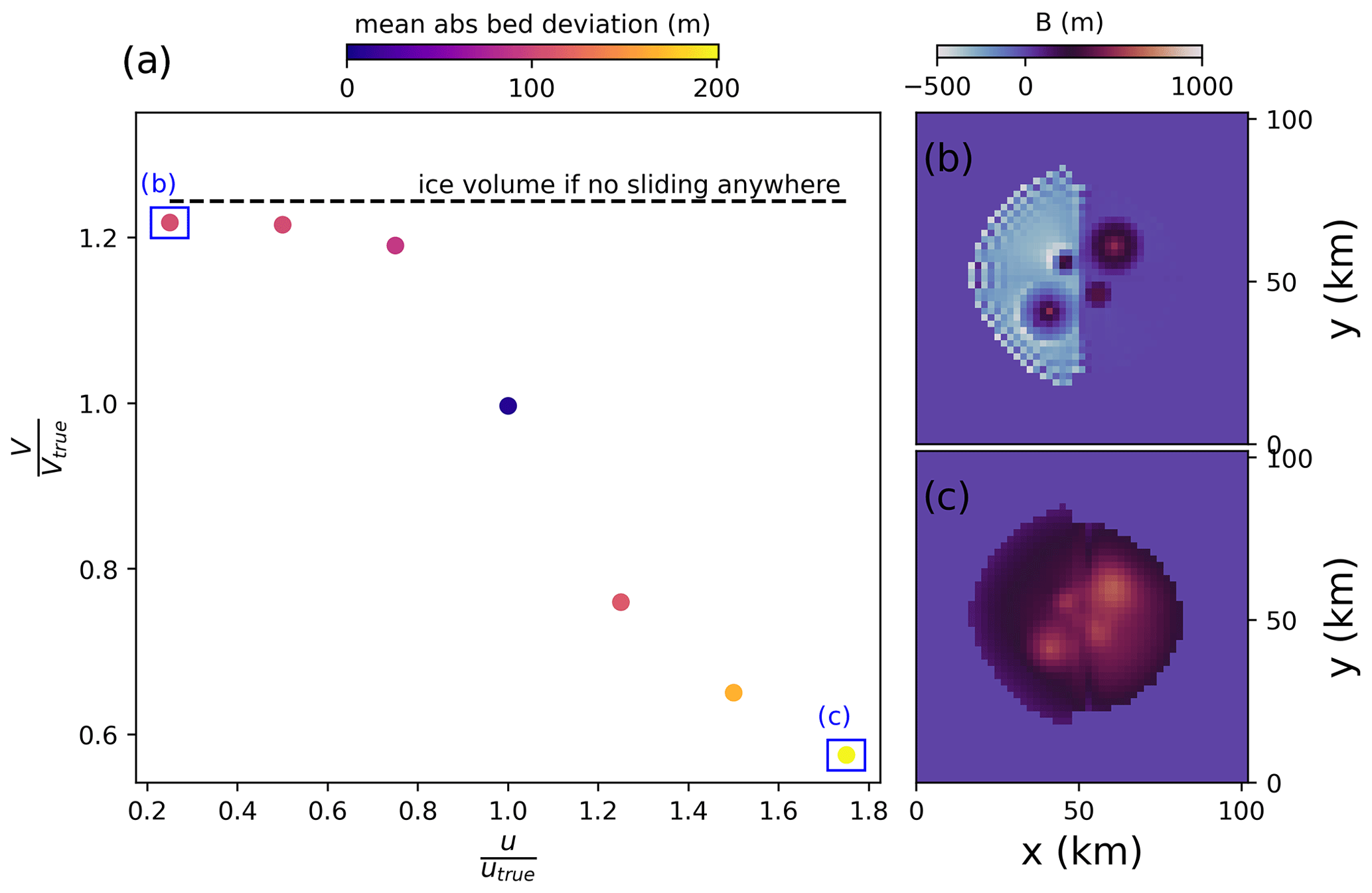
Figure A2 (a) Modelled ice volume after the inversion relative to the true ice volume of the ice cap as a function of velocity perturbations. Colours indicate the mean absolute deviation between the inverted bed and the true bed. The dashed line denotes the ice volume if the inversion is run without allowing any sliding anywhere; the final inverted bed topography for the largest positive and negative (i.e. ±75 %) velocity perturbations is shown in panels (b) and (c), respectively.

Furthermore, we simulate how errors in the glacier surface shape translate into bed errors. To that end, we add random noise with standard deviations of 5, 10, 15, 25 and 50 m to the ice cap surface. From theory, it is well known that surface shape errors can lead to large bed elevation errors since bed undulations typically leave a surface expression that is only a fraction of their magnitude (Raymond and Gudmundsson, 2005; Habermann et al., 2012; Bahr et al., 2014). Even a small surface bump, therefore, will be interpreted as a large bed undulation by the inversion. Generally, this effect is stronger for thicker and non-sliding ice, while thin sliding ice is affected to a lesser degree. Smoothing of the input data or regularization tools (e.g. Eq. 3) can mitigate problems arising from surface noise. To show the unmitigated effects of surface noise for the purpose of this sensitivity analysis, we do not smooth the input data and only apply the same weak regularization as in all other experiments shown here by setting the parameter θ=2.5 % in Eq. (3). Indeed, Fig. A3 demonstrates that, already with little surface noise, considerable bed noise is introduced, although the general bed shape can still be seen. As predicted by theory, the sliding (left) half of the domain is less affected than the non-sliding right half. For large surface noise, the bed shape is essentially unrecognizable, as is exemplified by a mean absolute bed deviation above 200. However, Fig. A3 also shows that the modelled ice cap volume is largely unaffected by surface noise, as is expected when the mass flux through the domain and the reference velocity field are unaltered.

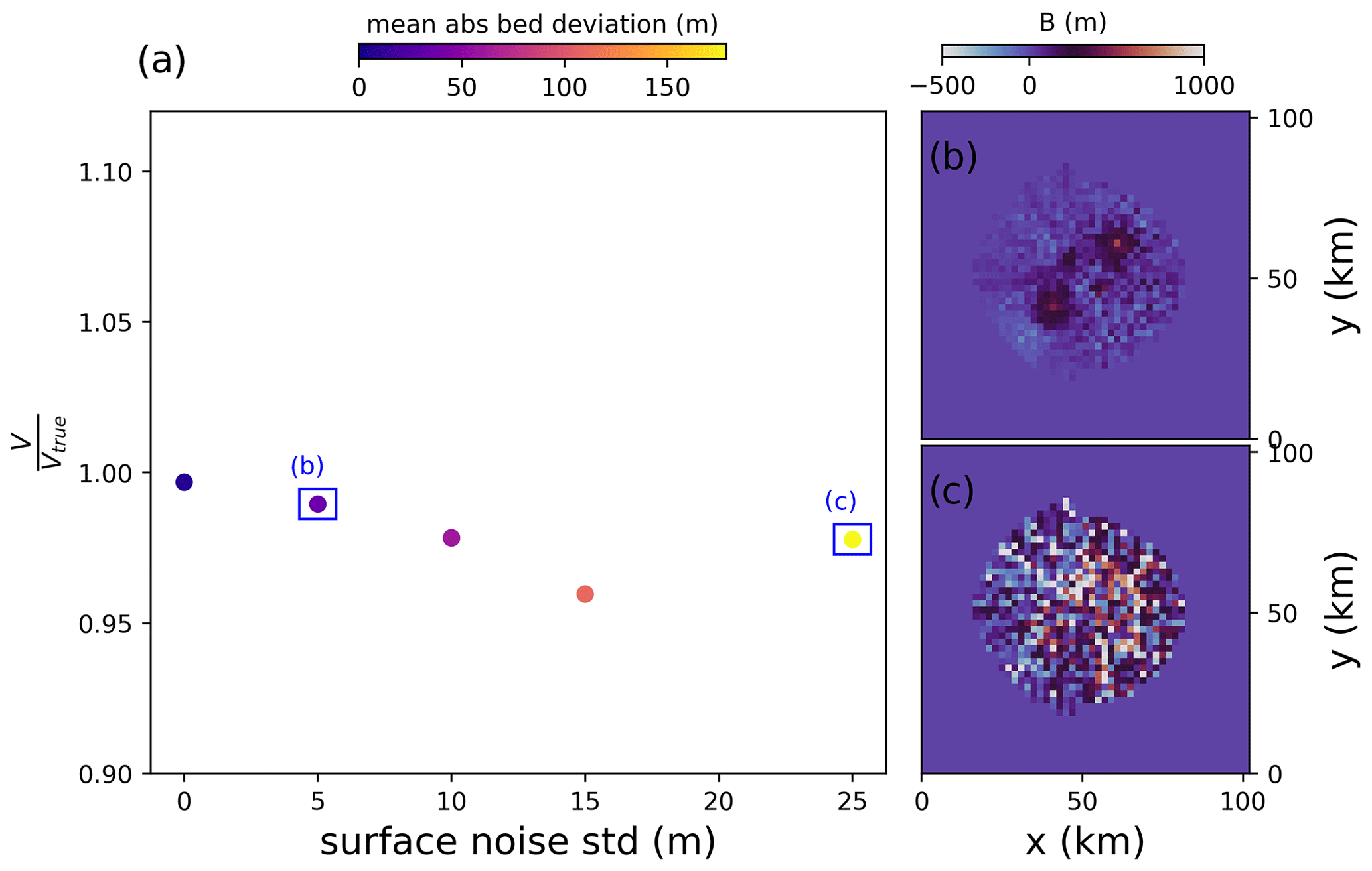
Figure A3 (a) Modelled ice volume after the inversion relative to the true ice volume as a function of surface shape perturbations with random noise. Colours indicate the mean absolute deviation between the inverted bed and the true bed; the final inverted bed topography for the smallest and largest surface shape perturbations is shown in panels (b) and (c), respectively.

Next, we consider ice temperature errors (Fig. A4). Specifically, we change the ice temperature from its true value (used to build the ice cap) of 268 K to values of 264, 266, 270 and 272 K. With the isothermal flow law used here, this means that the ice is uniformly made stiffer or softer as compared to its true viscosity. Colder ice deforms less, and so a thicker ice cap can be expected from a negative ice temperature error, whereas the opposite is the case for a positive ice temperature error. However, the results of the perturbation analysis suggest that this is not the case. Rather, only small errors in the final ice volume below 10 % are introduced by perturbing ice temperature. This is because the friction updates compensate for too-stiff or too-soft ice by reducing the sub-glacial friction if the ice is too slow, by thinning the glacier or by increasing friction if the ice is too fast (again, however, if there is no sliding at all, this does not have any effect). Indeed, when prescribing the true friction field at the start of the inversion and not applying any updates to it, larger errors in final ice volume are apparent for both too-cold and too-warm ice, as compared to when friction updates were enabled (Fig. A4).

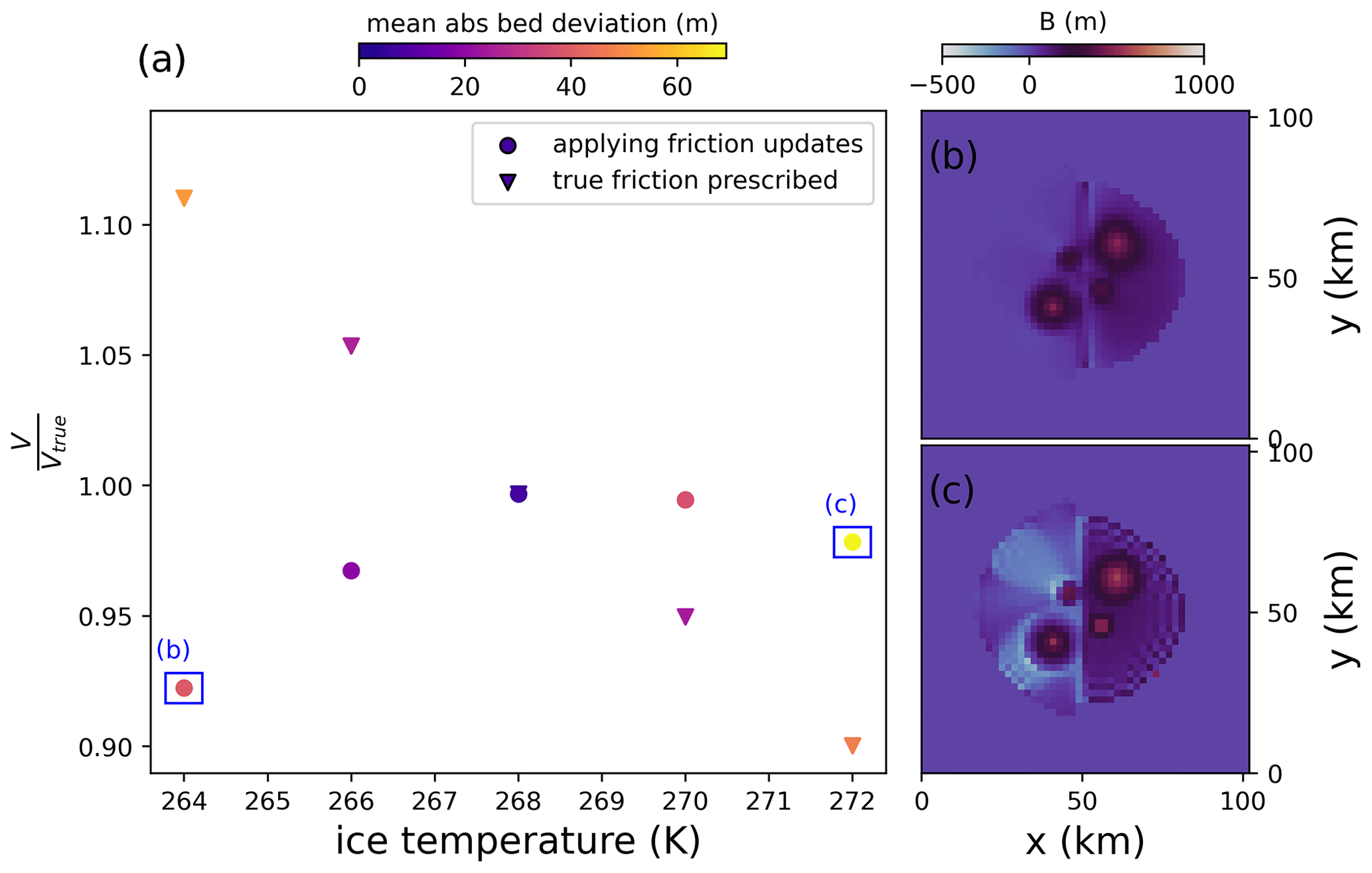
Figure A4 (a) Modelled ice volume after the inversion relative to the true ice volume of the ice cap as a function of ice temperature perturbations. Colours indicate the mean absolute deviation between the inverted bed and the true bed. Triangles represent runs where the true friction field was prescribed from the start of the inversion, meaning that no friction updates were applied. Dots denote runs where the friction field was not known a priori, and therefore friction updates according to Eq. (2) were applied; the final inverted bed topography for the largest positive and negative (i.e. 264 and 272 K, respectively) ice temperature perturbations when friction updates are applied is shown in panels (b) and (c), respectively.

A2 Inversion parameters

We now investigate how different parameter choices for the inversion influence results. We first look at different values for the length dt of the ice flow forward simulation. We explore values of 1, 0.5, 0.25, 0.15, 0.05, 0.025 and 0.01 years. Our results show virtually no difference in the final bed shape or remaining bed misfit (Fig. A5), such that using small values for dt can be used to save computational time.

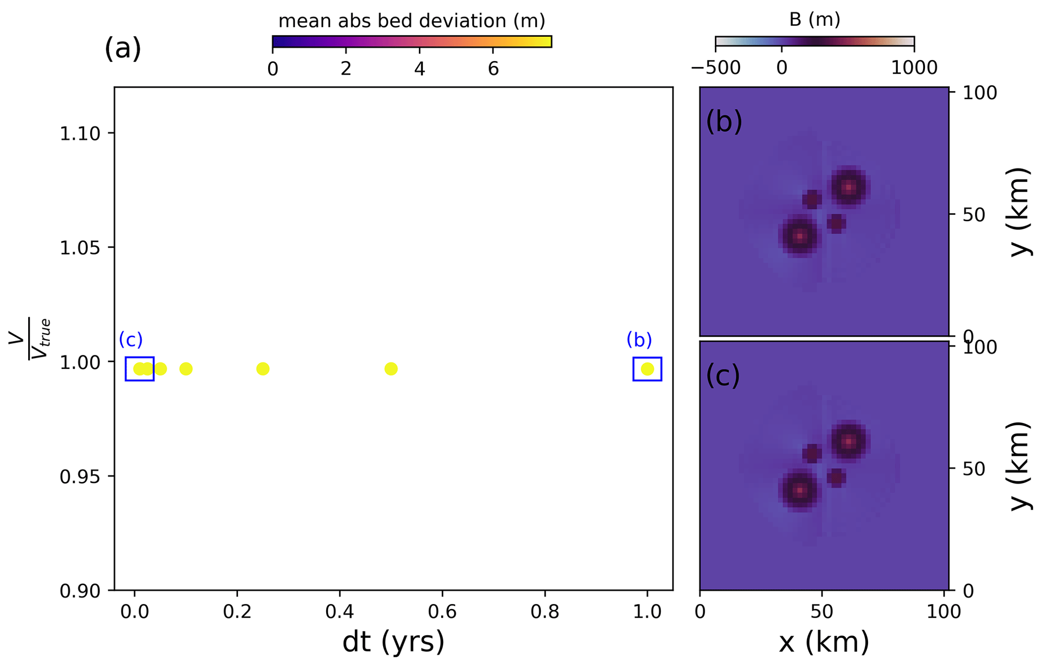
Figure A5 (a) Modelled ice volume after the inversion relative to the true ice volume of the ice cap as a function of different values for the forward-modelling time step dt. Colours indicate the mean absolute deviation between the inverted bed and the true bed; the final inverted bed topography for the smallest and largest dt (i.e. 0.01 and 1 year, respectively) is shown in panels (b) and (c), respectively.

Furthermore, we investigate different values for the relaxation parameter β in Eq. (1) (Fig. A6). β scales the $\mathrm{d}h/\mathrm{d}t$ misfit into bed corrections. Note that, for these experiments, we do not apply bed averaging. If β is large, the inversion should progress faster, but smaller bed features might not be resolved since they are overcompensated for, resulting in a bed oscillating around its true value during the iterations. Conversely, a small β slows down the inversion but results in a better resolved bed. Our sensitivity experiments confirm this. Indeed, with a larger β, the bed misfit (Eq. 7) is quick to converge towards a constant value after each friction update, while this is substantially slower for small β. However, the final inverted bed has a larger remaining misfit for a large β than a small β (Fig. A6).

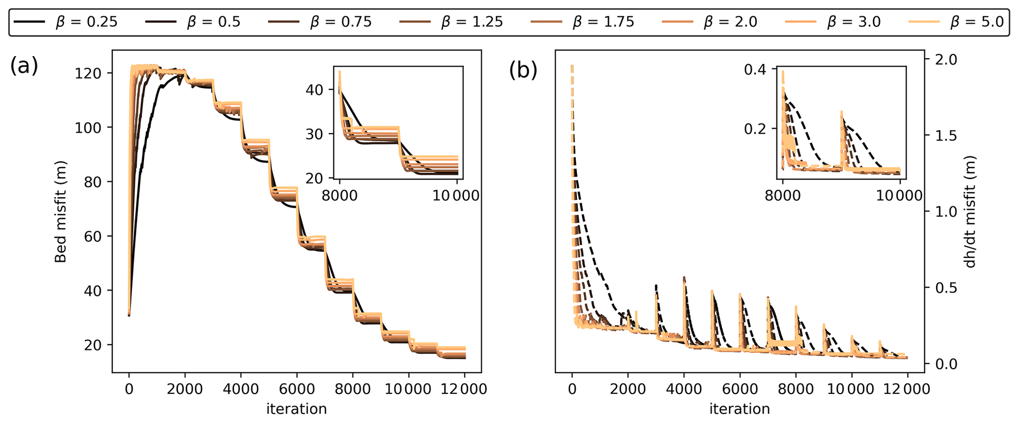
Figure A6 Sensitivity of bed inversion to the parameter β (Eq. 1). (a) Bed misfit per iteration step; (b) $\mathrm{d}h/\mathrm{d}t$ misfit per iteration step. The inset plots show zooms to iterations 8000 to 10 000. Sharp steps (a) or peaks (b) occur when friction updates are applied.

Now, we investigate different choices of the regularization parameter θ in Eq. (3) (Fig. 4). As discussed previously, θ serves the purpose of both regularizing the solution and allows the inversion to converge when input data and model physics otherwise cannot balance, e.g. due to errors in the input data that are not reproducible with ice flow physics. In the presence of larger errors, a larger θ will be required, because this gives the model flexibility to accommodate these erroneous observations. The choice of θ may thus be regarded as a measure of how well the ice flow model is deemed able to reproduce observations. At the same time, however, a larger θ also increases the dependence on initial conditions because it means that a larger part of the $\mathrm{d}h/\mathrm{d}t$ misfit is not accommodated with bed updates but with surface adjustments. We start by testing the regularization effect of θ by varying it without perturbing the input data. We test values of 0, 0.01, 0.025, 0.05, 0.1 and 0.3 for θ. The results show that, without any surface updates (i.e. θ=0), small-scale bed irregularities are introduced into the solution. They are too small to leave any noticeable impression on ice dynamics or surface shape, and so the inversion is not wrong in producing them; from the available surface “observations”, it is impossible to tell whether these features exist or not. However, it is generally undesirable to include features in the solution if they are not justified by the input data, and so regularization is in order. With increasing θ, the computed bed becomes smoother. However, this eventually comes at the cost of detail in the solution. For θ=0.3, the bed highs are no longer sharply visible. Next, we test how different choices of θ influence the inverted bed in the presence of input data errors. We investigate this here by applying the different values for θ to our ice cap, where the surface shape was perturbed by adding random noise with a standard deviation of 5 m. In this case, the forward model crashes since it cannot accommodate the perturbed surface shape if θ=0, whereas increasing θ helps to eliminate some of the surface noise. Again, though, when θ is too large, the bed is smooth but is also largely devoid of its characteristic topographic highs (Fig. 4). Note that the computed ice volume is always within 1 % of the true ice volume regardless of θ.

Finally, we also test whether a different initial bed guess influences the results. To that end, we assume that the ice thickness is zero everywhere in the domain at the start of the inversion. We find that this has no significant impact on the recovered bed (not shown). Likewise, a different initial guess for the friction field (i.e. we assume that it is slippery everywhere) does not change the bed solution. This suggests that our inversion is relatively stable towards initial conditions, although this is dependent on the choice of θ as described above.

A3 ITMIX glaciers

Supplementary plots for the three ITMIX glaciers tested (Sect. 5) are shown in Figs. A7–A9.

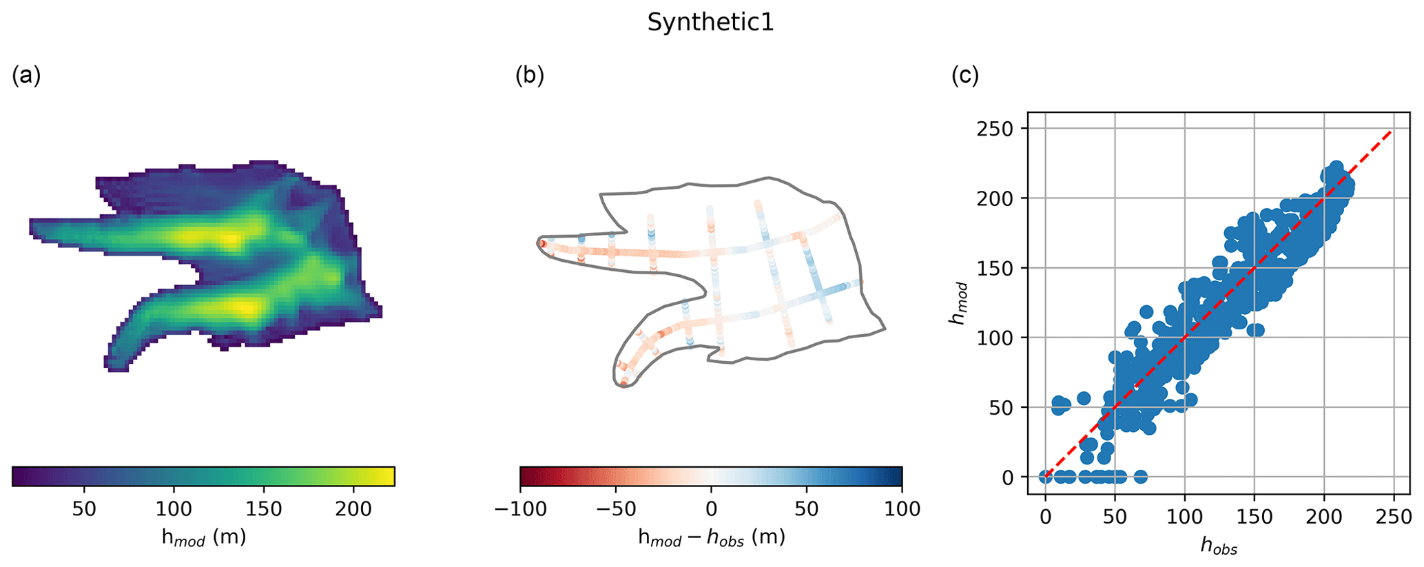
Figure A7 Inversion results for ITMIX glacier synthetic1 (Farinotti et al., 2017). (a) Modelled ice thickness; (b) modelled minus “observed” ice thickness along artificial “radar tracks”; (c) correlation between observed and modelled ice thickness.

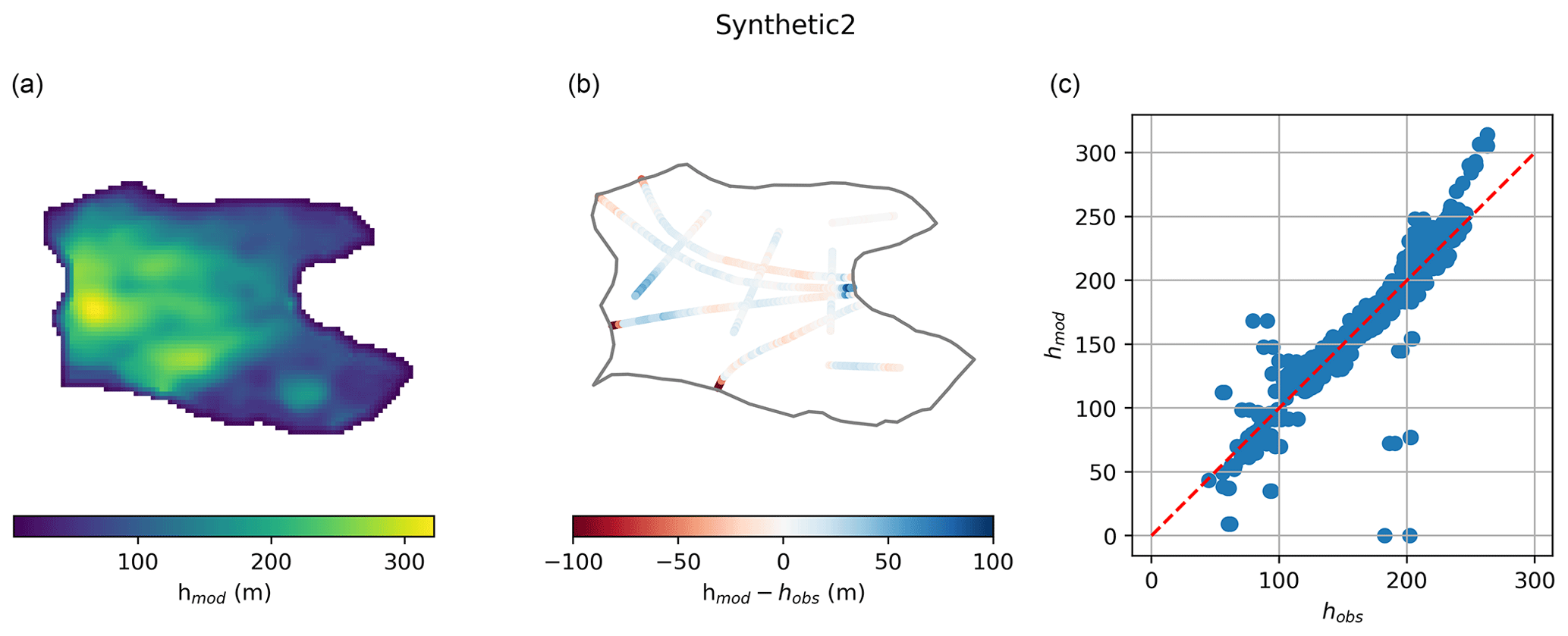
Figure A8 Inversion results for ITMIX glacier synthetic2 (Farinotti et al., 2017). (a) Modelled ice thickness; (b) modelled minus observed ice thickness along artificial radar tracks; (c) correlation between observed and modelled ice thickness.

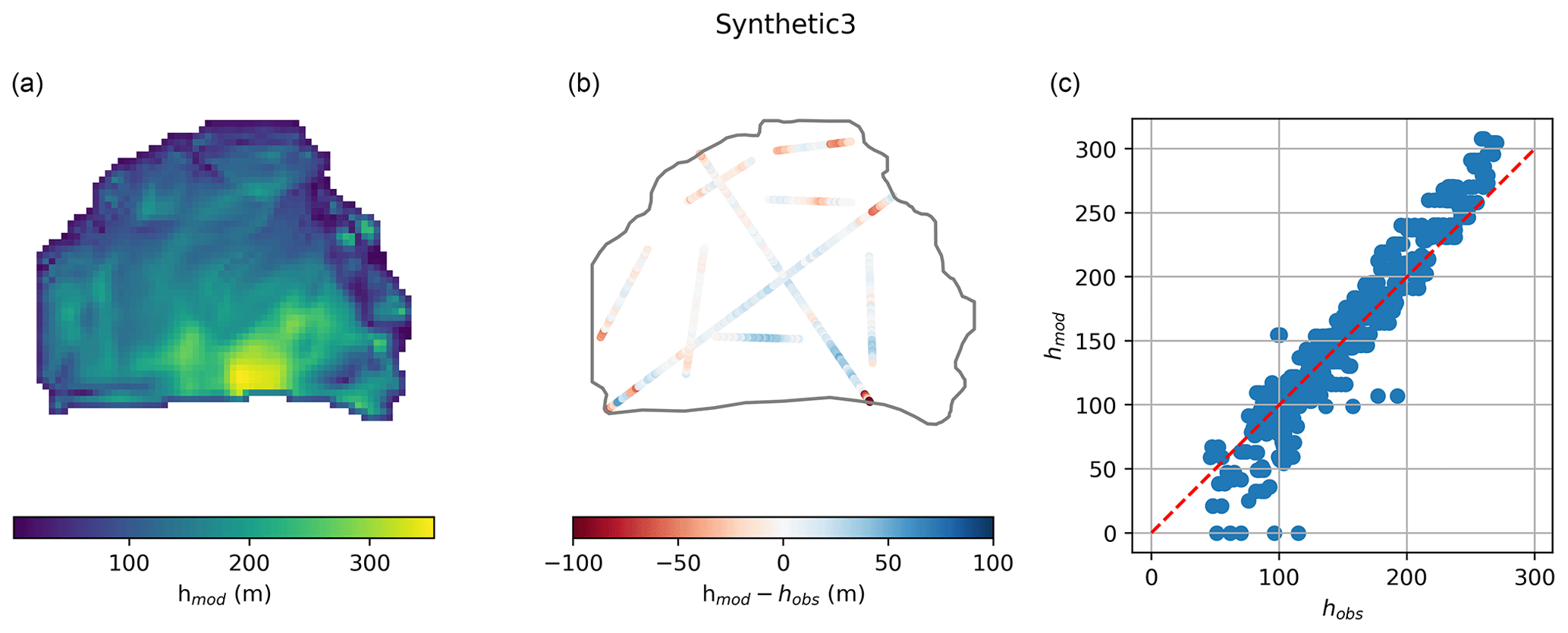
Figure A9 Inversion results for ITMIX glacier synthetic3 (Farinotti et al., 2017). (a) Modelled ice thickness; (b) modelled minus observed ice thickness along artificial radar tracks; (c) correlation between observed and modelled ice thickness.