the Creative Commons Attribution 4.0 License.
the Creative Commons Attribution 4.0 License.
 | 13 Sep 2023
Atmospheric drivers of melt-related ice speed-up events on the Russell Glacier in southwest Greenland
Valentina Radić
Andrew Tedstone
James M. Lea
Stephen Brough
Mauro Hermann
The Greenland Ice Sheet is a major contributor to current and projected sea level rise in the warming climate. However, uncertainties in Greenland's contribution to future sea level rise remain, partly due to challenges in constraining the role of ice dynamics. Transient ice accelerations, or ice speed-up events, lasting from 1 d to 1 week, have the potential to indirectly affect the mass budget of the ice sheet. They are triggered by an overload of the subglacial drainage system due to an increase in water supply. In this study, we identify melt-induced ice speed-up events at the Russell Glacier, southwest Greenland, in order to analyse synoptic patterns driving these events. The short-term speed-up events are identified from daily ice velocity time series collected from six GPS stations along the glacier for each summer (May–October) from 2009 to 2012. In total, 45 ice speed-up events are identified, of which we focus on the 36 melt-induced events, where melt is derived from two in situ observational datasets and one regional climate model forced by ERA5 reanalysis. We identify two additional potential water sources, namely lake drainages and extreme rainfall, which occur during 14 and 4 out of the 36 melt-induced events, respectively. The 36 melt-induced speed-up events occur during synoptic patterns that can be grouped into three main clusters: (1) patterns that resemble atmospheric rivers with a landfall in southwest Greenland, (2) patterns with anticyclonic blocking centred over southwest Greenland, and (3) patterns that show low-pressure systems centred either south or southeast of Greenland. Out of these clusters, the one resembling atmospheric river patterns is linked to the strongest speed-up events induced by 2 to 3 d continuously increasing surface melt driven by anomalously high sensible heat flux and incoming longwave radiation. In the other two clusters, the net shortwave radiation dominates the contribution to the melt energy. As the frequency and intensity of these weather patterns may change in the warming climate, so may the frequency and intensity of ice speed-up events, ultimately altering the mass loss of the ice sheet.
- Article
(7701 KB) - Full-text XML
-
Supplement
(2623 KB) - BibTeX
- EndNote


Mass loss from the Greenland Ice Sheet (GrIS) is a major component of sea level rise observed in recent decades (Kjeldsen et al., 2015) and predicted in climate projections (Goelzer et al., 2020). However, large uncertainties in Greenland's contribution to future sea level rise remain, partly due to challenges in representing ice dynamics that affect the GrIS mass budget through the discharge of ice to the ocean from outlet glaciers (Le clec'h et al., 2019). These dynamic losses account for approximately half of the mass loss observed in recent years, with the other half attributed to increased meltwater runoff (The IMBIE Team, 2020). Ice dynamics also affect the mass budget indirectly by redistributing ice towards the margins, causing an inland expansion of the ablation zone (Zwally et al., 2002; Bartholomew et al., 2011a; Shannon et al., 2013) and enhanced melting as ice advances to lower elevations with higher temperatures (Chu, 2014). Recent observational studies show a nonexistent or slightly negative correlation between summer melt and mean annual ice velocities in Greenland (Tedstone et al., 2015; Stevens et al., 2016). Nevertheless, it has been shown theoretically (Schoof, 2010) and has been observed (e.g. Zwally et al., 2002; van de Wal et al., 2008) that a short-term increase in water supply to the glacier bed can trigger a speed-up of the glacier. Thus, weather patterns that drive a substantial increase in surface melt production or are linked to extreme rainfall can trigger local short-term accelerations in ice flow (van de Wal et al., 2008; Shepherd et al., 2009; Doyle et al., 2015). As the occurrence and intensity of these weather patterns may change in the warming climate (Schuenemann and Cassano, 2010), so may the frequency and intensity of the ice speed-up events.
Ice dynamics in land-terminating glaciers at the GrIS margin are driven by the interplay between meltwater input and the evolution of the subglacial drainage system, similar to mountain glaciers (Shepherd et al., 2009; Chandler et al., 2013; Nienow et al., 2017). Meltwater can access the ice sheet bed through crevasses, supraglacial lake hydro-fracture, and moulins (Chu, 2014), increasing pressure in a thin layer of subglacial water and allowing faster basal sliding along the bed (Zwally et al., 2002). The impact of increasing meltwater input on ice velocities depends largely on the state of the subglacial drainage system which evolves dynamically between two main configurations: an inefficient drainage system (e.g. linked cavities) versus an efficient drainage system (e.g. ice-incised channels). High meltwater input into an inefficient subglacial drainage system causes a rapid ice acceleration, typically observed at the start of the melt season (van de Wal et al., 2008; Fitzpatrick et al., 2013). These speed-up events exhibit behaviour similar to “spring events” at Alpine glaciers (Mair et al., 2003; Shepherd et al., 2009; Bartholomew et al., 2011a; Chandler et al., 2013) as surface meltwater reaches the glacier bed for the first time in a year through existing crevasses and moulins. At higher elevations (>1000 m) on the Russell Glacier, spring events are shown to be less distinct or absent, reflecting the shift to a hydro-fracture-dominated environment through thicker ice (Bartholomew et al., 2012). In contrast to the inefficient drainage system, continuously high rates of water supply promote a channelized system, which in turn reduces water pressure and can even decelerate ice flow (Bartholomew et al., 2010). Both observations and theory, however, have shown that the ice speed-up events can also occur after a channelized subglacial drainage system has evolved (Bartholomew et al., 2010; Schoof, 2010). High-resolution ice velocity measurements in land-terminating sections of the southwestern GrIS reveal variability on three temporal timescales: diurnal cycles; seasonal cycles; and “event-type” accelerations of roughly 1 d to 1 week in duration (Hoffman et al., 2011; Bartholomew et al., 2012), henceforth referred to as ice speed-up events. These speed-up events are generally triggered by sudden surges in water input caused by lake drainage events or atmospheric conditions that induce high surface melt and/or rainfall.
The North Atlantic is a region with large weather variability driven by the interplay of the jet stream, synoptic-scale waves, ocean–land and north–south temperature contrasts, and large-scale flow modification due to orographic forcing of the Rocky Mountains (Rivière and Orlanski, 2007; Brayshaw et al., 2009). Surface melt on the GrIS is highly sensitive to this variability in atmospheric forcing (Hanna, 2005; Fettweis et al., 2013), with southerly warm-air advection as the main driver of large-scale GrIS melt events (Hermann et al., 2020). Phenomena related to the southerly advection are narrow corridors of intense water vapour transport known as atmospheric rivers (ARs), which frequently cause melt of the western GrIS through enhanced longwave radiation and sensible heat flux (SHF) (Mattingly et al., 2018, 2020). ARs typically occur along the cold front in warm sectors of extratropical cyclones due to moisture convergence and typically induce precipitation (Dacre et al., 2015; Sodemann et al., 2020). Slow-moving mid- to upper-tropospheric anticyclones, so-called blocking (Woollings et al., 2018), have also been linked to increased GrIS surface melting due to warm-air advection and reduced cloud cover which increases downward shortwave radiation (Hofer et al., 2017). A climate with frequent blocking, as has been observed in the past 2 decades, could double the GrIS mass loss due to increased summer melting (Delhasse et al., 2018). Climate change has the potential to alter these atmospheric circulation patterns in the North Atlantic, including a northward shift of the storm track (Schuenemann and Cassano, 2010) and increased water vapour transport in high latitudes (Lavers et al., 2015). In addition, the feedback mechanisms between Arctic warming and the jet streams (Francis and Vavrus, 2012; Barnes and Screen, 2015) could also be altered, potentially modifying high-frequency variability in melt and rainfall over the GrIS and, therefore, the occurrence of ice speed-up events.
One of the most well-studied regions of the GrIS, in terms of the ice speed-up events, is the Russell Glacier in the southwest of the ice sheet, also referred to as the “K transect” (van de Wal et al., 2008; Smeets et al., 2018). The region is representative of a large part of the GrIS margin, characterized by land-terminating glaciers, many supraglacial lakes, and summer melting (Shepherd et al., 2009). The K transect has been the subject of studies focused on ice dynamics and their links to atmospheric forcing, particularly the forcing of surface melting (van de Wal et al., 2008; Bartholomew et al., 2012; Tedstone et al., 2013). In addition to rainfall and surface melt, rapid drainages of supraglacial lakes have the potential to cause the sudden increase of water supply into the subglacial drainage system (Clason et al., 2015). Selmes et al. (2011) identified southwest Greenland as the region with the most fast-draining lakes (61 % of all lake drainage events on the GrIS from 2005 to 2009), and notably, rapid lake drainages on the Russell Glacier have been observed and linked to some short-term ice velocity accelerations at higher-elevation stations (Bartholomew et al., 2011a).
Despite the relatively large number of studies that have focused on ice dynamics at the K transect, systematic analysis of the links between the ice speed-up events and synoptic patterns has not been performed. In this study, we identify characteristic synoptic patterns linked to the speed-up events, based on the clustering algorithm known as self-organizing maps (SOMs). Once the patterns are identified, we apply a Lagrangian trajectory model to analyse their 5 d backward trajectories. The Lagrangian perspective is a particularly useful addition, e.g. to identify atmospheric flow features such as foehn (Elvidge and Renfrew, 2016), to understand atmospheric processes driving temperature extremes (Röthlisberger and Papritz, 2023), and to link synoptic patterns with the thermodynamic processes relevant for Arctic (Wernli and Papritz, 2018) and GrIS surface melt (Hermann et al., 2020). Here, the trajectory analysis (Sect. 4.3) provides a process-based link between the synoptic patterns (i.e. SOM clusters) during melt-induced ice speed-up events (Sect. 4.2) and the local conditions observed at the Russell Glacier (Sect. 4.4). As climate change will potentially bring substantial changes to weather systems and their variability, impacting the ice dynamics of this region, it is important to better understand current atmospheric drivers of the speed-up events in this region. This study aims to close this knowledge gap, in particular by identifying melt-induced ice speed-up events and investigating synoptic patterns that are linked to these events.
The Russell Glacier in the southwest Greenland Ice Sheet (SW GrIS) is located at 67∘ N near the settlement of Kangerlussuaq in a region often referred to as K transect (van de Wal et al., 2008). The area is well covered with glaciological and meteorological in situ observations (Fig. 1), including a 4-year time series (2009–2012) of ice velocity measurements at high temporal resolution (Sect. 2.1). Since the melt season at the Russell Glacier extends from May to late September or early October (van den Broeke et al., 2011) and no high-resolution ice velocity data are available outside this period, our analysis focuses exclusively on observations from May to October. These observations include ice velocity data, meteorological data needed for an assessment of surface melt through the surface energy balance, and observations of lake drainage events. The following sections provide more details on each of the datasets.
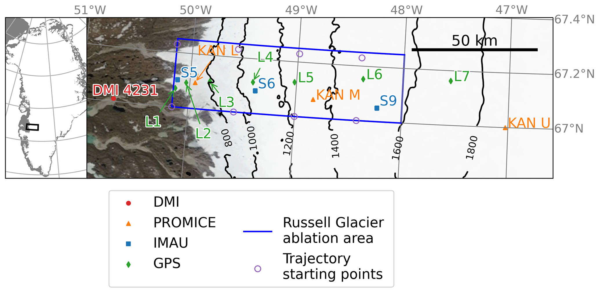
Figure 1The Russell Glacier area with measurement sites: L1–L7 are GPS sites; S5, S6, and S9 are automated weather stations maintained by IMAU; KAN L, KAN M, and KAN U are AWSs maintained by PROMICE; and DMI 4231 is a rain gauge maintained by the Danish Meteorological Institute. The approximate ablation area of the glacier is within the boundaries marked in blue. The starting points of the backward trajectories (see Sect. 3.5) are indicated with purple circles. The background is a NASA Modis/Terra satellite image on 3 June 2008, and black contours showing topography are produced from a digital elevation model of the Greenland Ice Mapping Project (Howat et al., 2014). The inset map on the left depicts the location of the study area on the GrIS.
2.1 Ice velocity data
Ice velocity measurements were made at seven sites (L1 to L7; Fig. 1) every summer from 2009 to 2012, using dual-frequency GPS receivers logging at 30 s resolution (Tedstone and Nienow, 2018). The data were kinematically corrected relative to an off-ice base station, and 6-hourly data are obtained by differencing positions across 6 h sliding windows, yielding results with <15 m yr−1 uncertainty (Bartholomew et al., 2011a). As this study does not focus on sub-daily variability, we average the ice velocities to daily values (in UTC−2), which reduces uncertainties to <3.7 m yr−1 (Bartholomew et al., 2011a).
Periods of missing data due to power failure occurred at all GPS sites, predominantly in autumn, and are treated as constant local ice velocities. Because this study focuses on short-term variability rather than absolute values, missing data at individual GPS sites is not a major issue. However, the amplitude of a daily-averaged ice speed-up event may be dampened if data are missing from a station that was in reality accelerating. Table S1 in the Supplement lists stations with missing data during each ice speed-up event. We removed an apparent velocity spike in GPS site L2 in October 2009 as the underlying position data show high scatter. Furthermore, GPS site L7, at 1716 m elevation, did not measure any significant ice accelerations, suggesting that no meltwater reached the glacier bed this far inland (Bartholomew et al., 2011a). Minor variability in horizontal velocities at this station can likely be attributed to coupling to ice downstream. Thus, L7 is excluded from this analysis, and we use the mean ice velocity of GPS sites L1–L6, termed Vice.
2.2 Melt and rainfall data
To assess surface melt at Russell Glacier, we use a combination of in situ observations of meteorological variables and surface energy fluxes, as well as a downscaled reanalysis dataset. The Institute for Marine and Atmospheric research Utrecht (IMAU) maintains three automated weather stations (AWSs; labelled S5, S6, S9; Fig. 1) that provided daily meltwater estimates from 2003 to 2012 based on a surface energy balance (SEB) model (van de Wal et al., 2015). The net SEB from this dataset is calculated as a sum of net longwave radiation (LWn), net shortwave radiation (SWn), latent heat flux (LHF), and sensible heat flux (SHF), where the latter two are estimated with the bulk aerodynamic method (Hay and Fitzharris, 1988). The available melt energy is then converted to meltwater production (hereafter: MIMAU), assuming a specific latent heat of 335 kJ kg−1 and an ice density of 900 kg m−3. In van de Wal et al. (2015), the daily mean errors in this method are estimated to be 5 %. To increase the spatial coverage and improve the robustness of surface melt estimates, we use a second, independent set of observations from three AWSs (labelled KAN L, KAN M, KAN U; Fig. 1) from the Programme for Monitoring of the Greenland Ice Sheet (PROMICE) (Fausto et al., 2021). The stations provide hourly measurements of air temperature (Ta), surface temperature (Ts), short- and longwave radiation (SWnet, LWnet), pressure, wind speed, and relative humidity (Fausto et al., 2022). From these data we estimate hourly turbulent heat fluxes (SHF, LHF) using the bulk aerodynamic method and subsequently calculate surface melt, MPROMICE, from the net SEB (see Sect. 3.1 for details on calculation). The methodology closely follows the melt model used for the IMAU data, but the PROMICE dataset additionally contains all SEB components separately and provides an estimate of cloud cover fraction based on downward LW radiation and air temperature.
As a third data source, we use daily outputs from the Modèle Atmosphérique Régional (MAR) version 3.11 at 10 km resolution (Gallé and Schayes, 1994; Fettweis, 2007) with lateral forcing from ERA5 reanalysis data (Hersbach et al., 2020). MAR is a regional climate model that focuses on the representation of physical processes in polar regions with a fully coupled snow energy balance model (Gallée and Duynkerke, 1997). Extensive evaluation (e.g. Fettweis et al., 2017; Sutterley et al., 2018) has shown that MAR represents current climate conditions in Greenland with high accuracy for near-surface temperature, melt, and SMB. From MAR, we use daily meltwater production (MMAR) averaged over the Russell Glacier ablation area (Fig. 1).
Rainfall measurement stations are sparse on the GrIS, and the only permanent and rain-gauge-equipped AWS in the vicinity of the Russell Glacier is station 4231 of the Danish Meteorological Institute (DMI). It provides 24 h precipitation sums (without distinction between solid and liquid) at 06:00 UTC (03:00 UTC−3, i.e. west Greenland time) (Cappelen, 2020). We estimate rainfall from total precipitation by setting values to 0 mm d−1 when the local daily mean air temperature is below 0 ∘C. As temperatures vary significantly with elevation and the diurnal cycle, this method introduces some error. Since the measurement station is located at 50 m a.s.l., lower than any point of the Russell Glacier, DMI rainfall can be interpreted as an upper-end estimate for actual rainfall on the glacier. A secondary rainfall data source is the MAR, averaged over the same area as for the surface melt (Fig. 1).
2.3 Lake drainages
Supraglacial lakes within the Russell Glacier ablation area (Fig. 1) are identified using the dynamic thresholding approach applied to daily MODIS satellite imagery (Selmes et al., 2011), allowing lakes of more than 2 pixels (0.125 km2) to be identified. Lakes that drain rapidly are identified from these data using the methodology of Cooley and Christoffersen (2017). The criteria used for identifying lake drainage as rapid require a drainage observation (a loss of either 90 % of the lake area or at least 1.5 km2, with less than 0.25 km2 remaining) between two sequential cloud-free images, separated by a maximum of 6 d. The conservative threshold of 6 d is chosen to minimize the number of missed events during multi-day periods without cloud-free satellite observations. However, it is possible that a slower lake drainage (>24 h) is falsely identified as rapid.
2.4 Synoptic-scale atmospheric data
All large-scale meteorological variables in this study come from ERA5 reanalysis data (Hersbach et al., 2020; Hersbach et al., 2023) provided by the European Centre for Medium-Range Weather Forecasts (ECMWF). ERA5 uses a hybrid incremental 4D data assimilation system with variational bias correction and provides hourly data on a 0.25 ∘ grid and 137 vertical levels. Delhasse et al. (2020) found that for almost all near-surface variables over Greenland, ERA5 outperforms its predecessor ERA-Interim which, until recently, was considered the best reanalysis over Greenland (Chen et al., 2011; Lindsay et al., 2014; Fettweis et al., 2017).
The variables used in this study are eastward and northward integrated vapour transport (IVT), sea level pressure (SLP), and geopotential height at 500 hPa (Z500), averaged to daily values in west Greenland time (UTC−3) from 1979 to 2020 at a horizontal resolution of 0.5∘. In addition, we identify spatial objects of atmospheric blocks and cyclones from 6-hourly ERA5 fields, which are then averaged to daily values in UTC−3. A block is identified in two steps according to Schwierz et al. (2004) and Croci-Maspoli et al. (2007): first, the 6-hourly anomaly (from the monthly climatological mean) of vertically integrated potential vorticity (PV) between 500 and 150 hPa has to be less than −1.0 pvu (potential vorticity unit; 1 pvu = 10−6 K m2 kg−1 s−1). Second, using an object-tracking algorithm, a block refers to such a PV anomaly that is additionally sustained over a period of at least 5 d. Hence, we characterize blocking as a pronounced and persistent negative PV anomaly in the upper troposphere. A surface cyclone is identified from the outermost closed SLP contour around a local SLP minimum as by Wernli and Schwierz (2006) and Sprenger et al. (2017). Importantly for the Greenland region, local SLP minima above 1500 m elevation are excluded due to the pronounced extrapolation required to compute SLP over strongly elevated topography. For details regarding the identification of both weather systems, we refer the reader to the provided references, whose approach we follow without exception.
3.1 Melt calculation from PROMICE data
As PROMICE stations have a sizable amount of missing hourly data on turbulent heat fluxes and melt, we use a simple SEB model to fill in those gaps. For hours with a surface temperature of 0 ∘C, the available melt energy is calculated as a sum of measured net longwave radiation (LWn), measured net shortwave radiation (SWn), and calculated sensible and latent heat fluxes. The latter two are calculated using the most commonly used bulk aerodynamic method based on the “K theory” or mixing-length theory (Stull, 1988):
where ρ is the density of air, cp=1005 is the specific heat capacity at constant pressure, is the latent heat of evaporation, and ϵ=0.622 is the ratio between the specific gas constant for dry air and water vapour. u is the measured wind speed at height z above the surface; p is the air pressure; and Tz and Ts are the measured temperatures at height z and at the surface, respectively. ez is the vapour pressure at the measurement height, which is calculated from relative humidity and temperature measurements using the improved Magnus formula (Alduchov and Eskridge, 1996). es is the vapour pressure at the surface, which is assumed to be at saturation (i.e. 610.78 Pa at 0 ∘C).
CT and Cq are the bulk transfer coefficients which are estimated using Monin–Obukhov similarity theory (Monin and Obukhov, 1954):
where k (i.e. 0.4) is the von Kármán constant and zu, zT, and zq are the measurement heights for wind (u), temperature (T), and humidity (q). Following the approach of Fausto et al. (2021), we use 0.001 m for the roughness length for momentum z0,u, and temperature and humidity roughness lengths are considered to have the same values assessed using the formulation from Smeets and van den Broeke (2008) for rough ice surfaces. The stability correction functions from Holtslag and De Bruin (1988) for stable conditions and Dyer (1974) for unstable conditions are calculated using an iterative method.
For days where the measurement of the sensor height (z) is available, our calculations for SHF and LHF correlate well (>0.99) and have a bias <1.5 W m−2 compared to the estimates from PROMICE. For the station KAN M, two longer data gaps in the measurement of the surface height of 1–1.5 months exist, but all other variables required to calculate turbulent heat fluxes, and SEB, are provided. Because changes in the surface height, as measured by a sonic ranger, are mostly gradual, we chose to fill these gaps by linearly interpolating the existing data.
3.2 Identification of speed-up events
Ice speed-up events along the K transect can differ substantially among the measurements stations (L1 to L6), with particular contrasts between lower elevations (L1–L3) and higher elevations (L4–L6). The speed-up events at the beginning of each melt season usually start at lower elevations, shifting towards higher elevations as melting intensifies, while the dynamic response at lower sites decreases. To show this contrasting spatial pattern, we apply a principal component analysis (PCA) on the ice velocity time series from the six stations (L1 to L6), an approach that was recently successfully applied to satellite-derived 2D ice velocity fields over the marine-terminating Jakobshavn Glacier in southwest Greenland (Ashmore et al., 2022). The results of our PCA yield eigenvectors for a total of six modes, each one showing the spatial pattern of normalized ice velocities across the stations (Fig. 2). The principal components (PCs) of each mode show its temporal pattern (time series), or in other words, the magnitude of the PCs shows the strength of the given spatial pattern in time. The first two modes carry the bulk of the variance in the data (84 %), and we therefore focus only on the first two modes (Fig. 2). The contrasting behaviour among the ice velocities measured at upper- versus lower-elevation stations is represented by the second mode, which accounts for 20 % of variance. The eigenvector of this mode shows a pattern of opposite signs between L1–L3 and L4–L6. The PCs of this mode reveal that the lower stations are more active (detecting movement) at the beginning of the melting season (large negative values of PCs in May), while upper stations can be more active towards the end of the season (large positive values of PCs in August and September). The leading eigenvector (first mode), explaining 64 % of the variance, correlates well with the mean ice velocity signal across all the stations (correlation coefficient of 0.98). This mode indicates that, to a large extent, all the stations experience the same temporal velocity signal, with the strongest amplitudes in L2 and L3. Thus, to simplify our identification of ice speed-up events, we use the spatially averaged velocity across the six sites (Vice).
To identify the speed-up events from this spatially averaged velocity time series, we define the event as a period with monotonically increasing ice velocity with a minimum increase of 13 m yr−1 per duration of the event. This threshold is chosen by visually determining the onset of the tail in a distribution of monotonic velocity increases per event (Fig. 3) and results in an identification of 45 ice speed-up events with durations of 1 to 8 d. None of the identified ice speed-up events occur in October due to a lack of strong melt or rainfall peaks and limited availability in GPS ice velocity data.
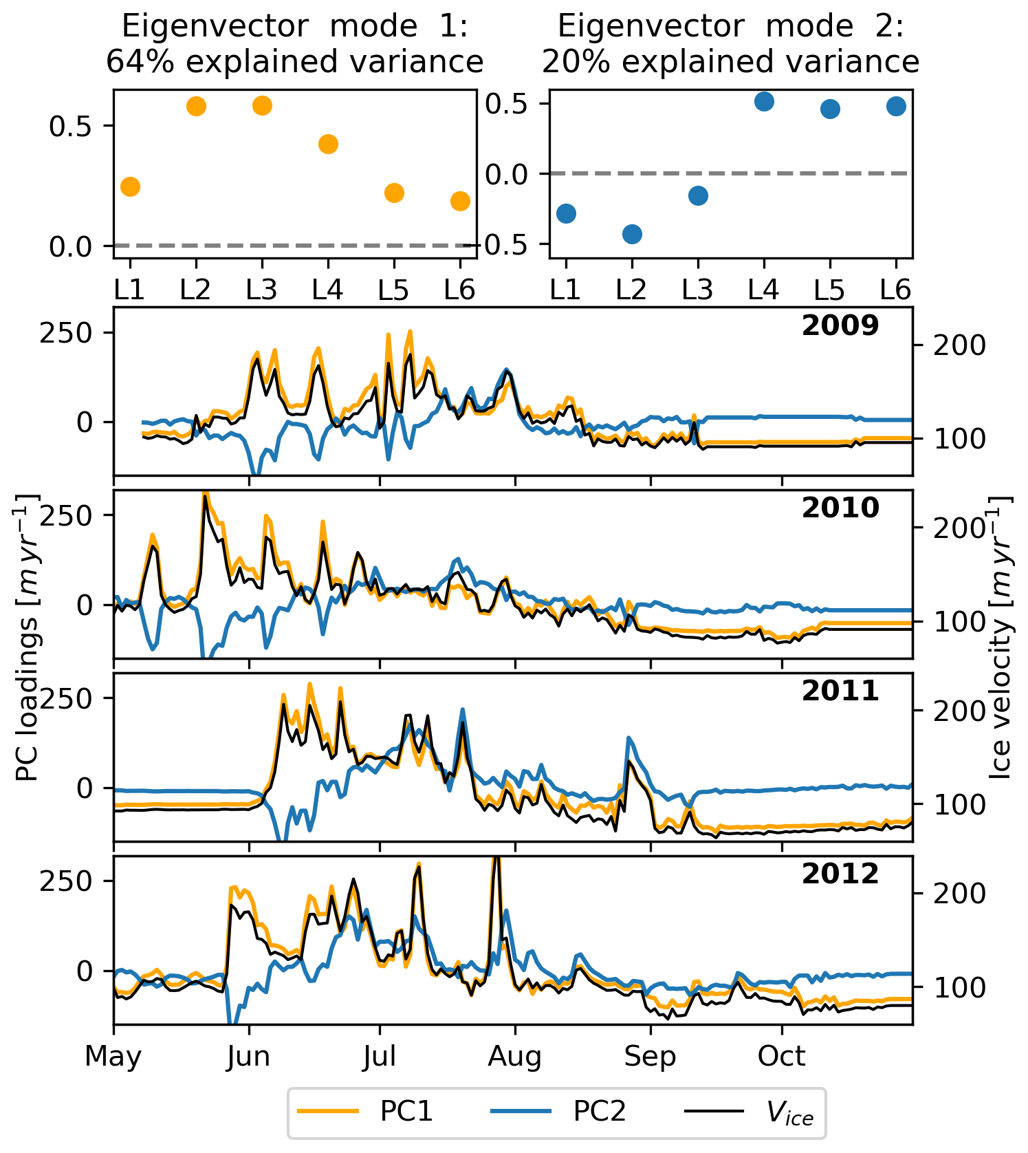
Figure 2Visualization of the first two modes of the PCA from the ice velocity data, which together account for 85 % of variance in the data. The top panel shows eigenvectors of the first two modes, and the panels below show the corresponding PCs (PC1 in orange and PC2 in blue) together with a time series of the mean ice velocity of GPS sites L1–L6, Vice (black).
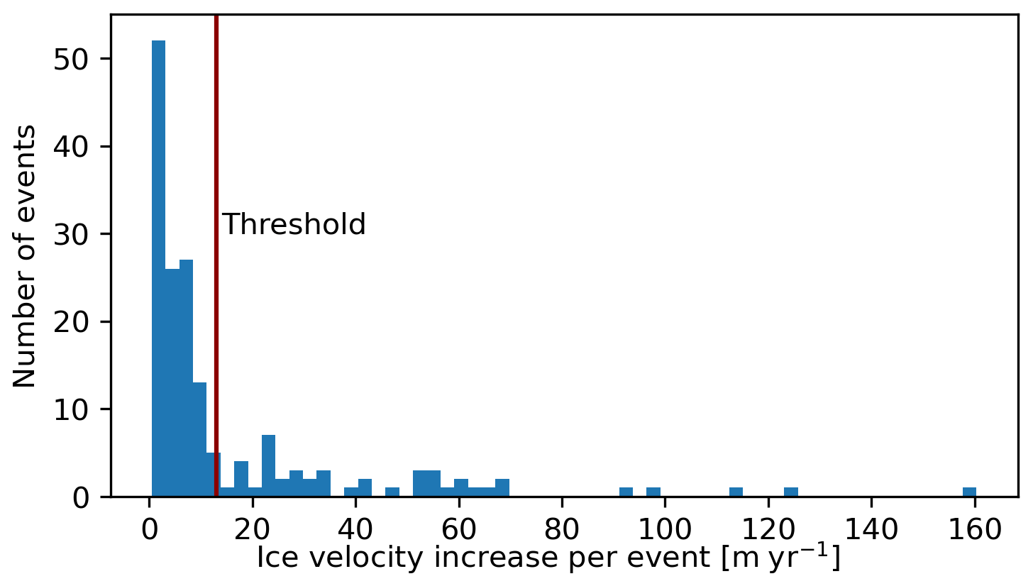
Figure 3Histogram of monotonic velocity increases per the duration of the speed-up event, derived as the difference between the maximum velocity at the end of the event and the minimum velocity at the start of the event. Each velocity increase above the threshold of 13 m yr−1 (in red) is considered to be an ice speed-up event.
3.3 Identification of melt events linked to ice speed-up events
For the analysis of atmospheric drivers, we focus solely on melt-induced ice speed-up events, which are identified as follows. First, cross-correlations are calculated, with lags of 0, 1, 2, and 3 d, between Vice and surface melt (MIMAU, MPROMICE, MMAR) for the 20 d moving windows from 1 May to 31 October for each of the 4 years (2009–2012). Figure 4 shows that the three different datasets (IMAU, PROMICE, and MAR) agree on the highest correlations between the velocity and melt time series at 0 or 1 d lags back in time, with <4 % cases with the highest correlations at 2 or 3 d lags back in time. The seasonal pattern of these correlations is not sensitive to the chosen window size between 10 and 30 d.
Second, we calculate the increase in melt that is consistent among the three melt datasets for each previously identified ice speed-up event. If the consistent melt increase persists over multiple days during the ice speed-up event, we focus on the day with the largest melt increase for the analysis of atmospheric drivers. This identified day for each ice speed-up event is hereafter referred to as the “melt increase day” (MI day), and the corresponding ice speed-up events are referred to as “melt speed-ups”. Daily increase in surface melt, rather than absolute melt, is considered because theory suggests that the short-term variability is critical to overloading the subglacial drainage system (Schoof, 2010). Based on the cross-correlation results, we allow for a maximum lag of 1 d between the melt increase and the start of the ice speed-up event to account for percolation through the snow cover or supra-/englacial water storage, which can delay the water delivery to the subglacial drainage system. Longer delays are also possible (particularly with water stored in supraglacial lakes), but these are addressed separately through the lake drainage identification.
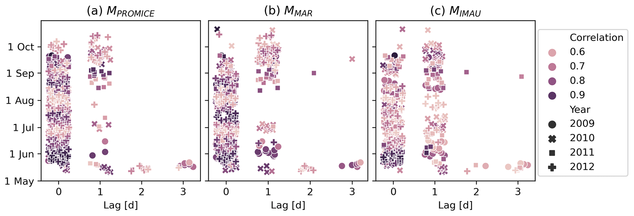
Figure 4The day of the year (DOY) versus the time lag in the cross-correlation between Vice and melt data from (a) MPROMICE, (b) MMAR, and (c) MIMAU, calculated for 20 d moving windows in May–October for 2009–2012. For each 20 d window one lag value is identified by the highest (lagged) correlation and is shown in the figure only if the correlation coefficient is larger than 0.5. DOY values in the figure mark the centre of each 20 d window. The colour of the points refers to the correlation value, while the marker of the points indicates the year.
3.4 Clustering of synoptic patterns
Prior to identifying the weather patterns that are linked to the melt-induced speed-up events, we first identify characteristic daily weather patterns occurring during the melting season (May–October) over a longer climatological period. To this end, we use self-organizing maps (SOMs) to cluster synoptic weather patterns represented as daily ERA5 IVT fields over a domain covering Greenland (50–85∘ N, 10–80∘ W) from May to October over a period of 42 years (1979–2020). SOMs are unsupervised machine learning methods capable of pattern recognition and clustering of multivariate datasets. Kohonen (2013) provides a detailed explanation of the algorithm, while technical details on the application of the SOM to IVT fields are provided in Radić et al. (2015). One of the advantages of the SOM over more traditional clustering techniques is its ability to organize the clusters (nodes) in a 2D map (SOM), with more similar patterns being placed closer together on the map, while dissimilar patterns are further apart (Liu and Weisberg, 2011). While the method is unsupervised, the user needs to choose the size of the final SOM, i.e. how many clusters to identify in the dataset, and set the tunable parameters (e.g. learning rate of the algorithm). We use IVT as an input variable, which has been identified as an important determinant of GrIS melt (Mattingly et al., 2016), because it not only characterizes warm–moist air advection, but also is linked to precipitation and cloud cover and, thus, the short- and longwave radiation budget (van Tricht et al., 2016).
After obtaining the final SOM, which gives us the characteristic IVT patterns placed on the map so that more similar patterns are closer together and more dissimilar ones are farther apart, we also perform a set of sensitivity tests. With these tests we assess how the SOM results vary as we change the size of the SOM (number of clusters), the size of the spatial domain, the variable used as input data (e.g. sea level pressure instead of IVT), and the tunable parameters in the SOM algorithm (see Schmid, 2021, for details on the sensitivity testing). Once the final SOM is determined by choosing a stable configuration that successfully captures a range of characteristic synoptic patterns over southwest Greenland, the occurrence of each IVT pattern (node) can be tracked in time and represented as time series (e.g. node identifier versus time). The patterns that occur during the MI day of each melt speed-up are considered to be the synoptic patterns linked to the ice speed-up events.
3.5 Trajectory calculation
To acquire a more in-depth understanding of the synoptic situation during melt-induced ice speed-up events, we calculate 5 d kinematic backward trajectories with the Lagrangian analysis tool LAGRANTO (Wernli and Davies, 1997; Sprenger and Wernli, 2015) for the MI day of each melt speed-up event. LAGRANTO allows for tracing the path of air backwards in time by numerically solving the trajectory equation (Eq. 5)
where x is the position of an individual air parcel and u the 3D wind vector.
Trajectories start at 09:00, 12:00, and 15:00 UTC−3 during each MI day on an equidistant grid (eight points; dx=25 km) within the Russell Glacier ablation area (Fig. 1), resulting in 3×8 trajectories per MI day. In the vertical, trajectories start at 10 and 30 hPa above ground level (combined and labelled surface), at 750 hPa (labelled lower troposphere), and at 500 hPa (labelled mid-troposphere). Along each trajectory, we trace the air mass' pressure (p), temperature (T), specific humidity (Q), and relative humidity (RH). All the variables, including the trajectory position in space, are output every 3 h.
4.1 Speed-up events
As stated in the last section, we identified in total 45 ice speed-up events. Most of these events have a duration of 1 to 4 d, with only three events that are up to 8 d long (Fig. 5). The increase in mean velocity Vice (final minus initial velocity) for these events ranges from 13 to 160 m yr−1. An increase in the mean velocity is typically a result of a local ice speed-up at two to four of the measurement sites. Thus, local amplitudes in the velocity signal at individual stations can be much higher than those in Vice, with the biggest recorded increase of 356 m yr−1 at the L2 site during the event starting on 16 May 2010. As the melt season progresses, a general shift from strong accelerations at low-elevation stations to higher-elevation stations is observed, as demonstrated with the PCA results (Fig. 2).
The first speed-up events of the melt season have distinct dynamics as meltwater reaches the glacier bed for the first time in a year (see Sect. 1), necessitating an explicit identification. We identified these local spring events from the low-elevation stations (L1–L3) as the first events with a velocity increase of more than 50 % above the March–April background velocity (Fig. 5). In 2010 and 2011, all low-elevation stations simultaneously show the spring events, while in 2009 and 2012 we observe a separate (earlier) spring event for the lowest site L1. These spring events include four of the nine strongest overall ice speed-up events (>60 m yr−1 increase) and two weaker events in 2009 and 2012 (Fig. 5).
To analyse potential drivers of the ice speed-up events, we plot the ice velocity time series together with the different sources of water that have the potential to overload the subglacial drainage system and accelerate the ice flow: surface melt, rainfall, and lake drainage events (Fig. 5). The three available surface melt datasets differ in absolute values (shaded blue in Fig. 5) partly due to the elevation bias in their spatial coverage. The mean melt over the whole period is 12.4 mm d−1 for PROMICE, 18.5 mm d−1 for IMAU, and 13.3 mm d−1 for MAR data. However, the day-to-day variability in melt, which is critical for the detection of speed-up events, agrees well with correlations over 0.9 (MAR-IMAU: 0.92, MAR-PROMICE: 0.97, IMAU-PROMICE: 0.95). Furthermore, mean ice velocities are strongly linked to surface melt with correlations of 0.7–0.75 between Vice and the three melt datasets. Out of the 45 ice speed-up events, 36 are identified as melt speed-ups (with the MI day marked in red in Fig. 5), while the remaining nine events are labelled “non-melt speed-ups”.
Relative to the average surface melt during the melt speed-ups, average rainfall values are over an order of magnitude smaller at 0.48 mm d−1 for DMI (which represents an upper-end estimate) and 0.40 mm d−1 for MAR data. The temporal variability in rainfall from the two datasets does not agree well, with a correlation of only 0.37. From the DMI and MAR datasets we estimate a daily increase in rainfall of >5 mm d−2 occurring for 10 ice speed-up events when considering the maximum of both rainfall datasets. However, only for 4 out of these 10 events does the rainfall amount exceed the increase in surface melt (Table S1 in the Supplement): 16 June 2010, 27 August 2010, 27 August 2011, and 5 July 2012 (Fig. 5), and only on 27 August 2010 do both rainfall datasets agree.
In addition to melt and rainfall, lake drainage events are also a potential driver of ice speed-up events (Fig. 5). In the considered time period, rapid drainage events of lakes between 0.1 and 6.9 km2 in size are observed on 65 d throughout May, June, and July. Out of the 45 identified speed-up events, 16 events co-occur with at least one rapid lake drainage (Fig. 5). Of these 16 events, 14 also coincide with a melt increase, while 2 events, both in late July 2009, can be attributed solely to the lake drainage, one with a total lake area of 4.69 km2 and the other with 4.75 km2.
Because lake drainage events are not directly linked to atmospheric conditions and the increase in surface melt dominates the daily rainfall magnitude, our analysis of atmospheric drivers focuses on melt speed-ups only (orange shaded in Fig. 5). Each of the 36 identified melt-induced speed-up events that can last from 1 to 8 d is associated with only 1 MI day identified as the day with the largest increase in daily melt (see Sect. 3.3). The MI day (red dot in Fig. 5) occurs 1 d before the onset of the ice velocity increase for three events (i.e. 8 %) and otherwise during the ice speed-up (33 events; 92 %). Notably, the MI day is mostly concurrent with the day of the largest increase in Vice (14 events; 38 %) or 1 d before the largest increase (17 events; 47 %).
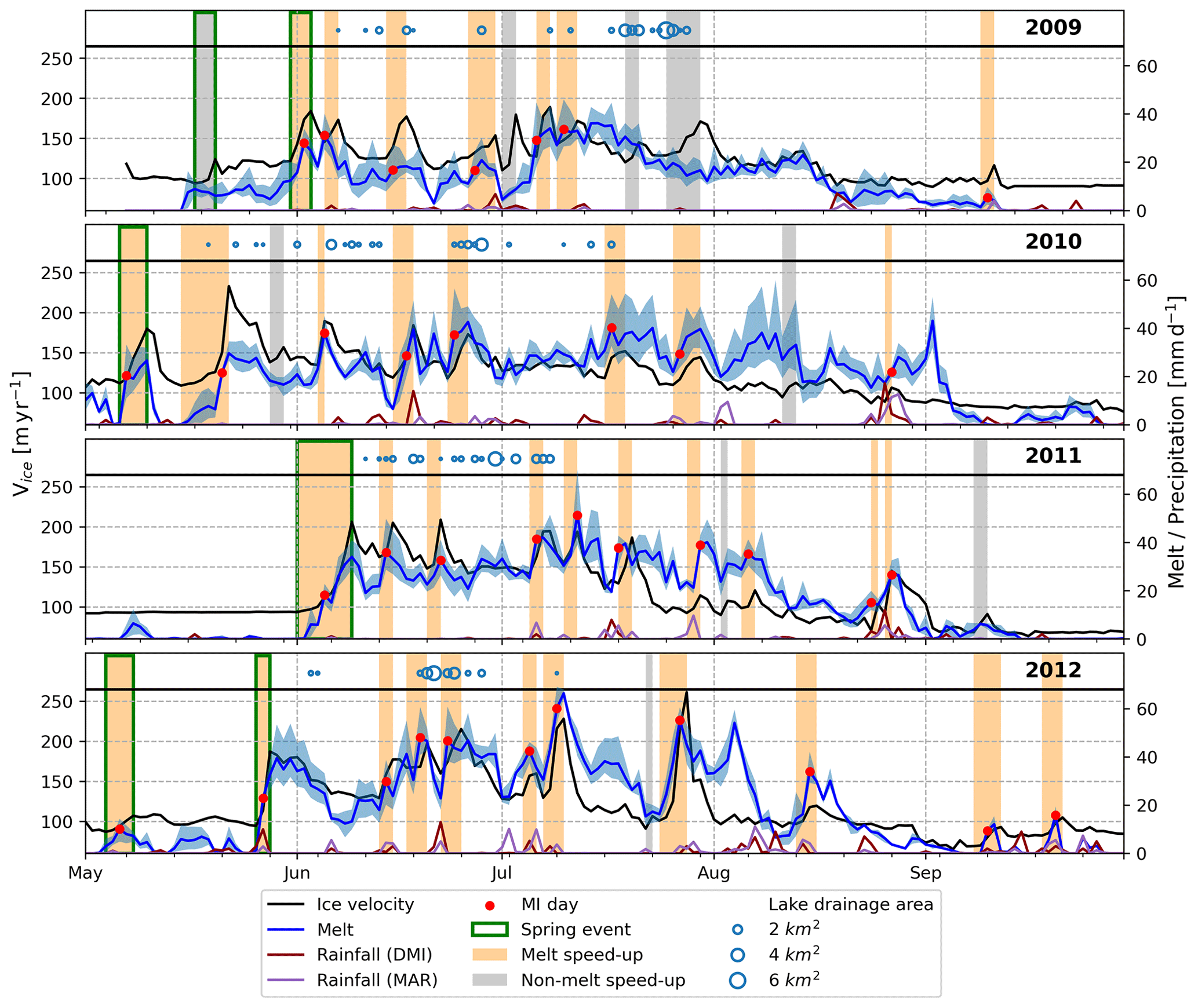
Figure 5Time series of the mean ice velocity Vice (black line), mean surface melt (blue line) with the full range of values from the three datasets (blue shaded area), and rainfall from the DMI station (brown) and from MAR (purple), all for the years 2009–2012 from May to September. October is not shown as no ice speed-ups occur after September. Melt increase days (MI days) are marked with red dots, while the corresponding 36 melt speed-ups are marked with orange shaded areas, and nine non-melt speed-up events are marked with grey shaded areas. For the exact durations of each ice speed-up event, see Table S1 in the Supplement. Spring events are marked with a green-lined rectangle, and rapid lake drainage events are marked with unfilled blue circles whose area represents the relative size (area in km2) of the lake that drained.
4.2 Synoptic patterns linked to ice speed-up events
Prior to identifying synoptic patterns that are linked to the melt speed-ups, we show the characteristic synoptic patterns, as fields of IVT over the large domain including Greenland, identified by the SOM algorithm. The method has produced 20 characteristic patterns of IVT fields, placed on the final 4×5 grid or SOM (Fig. 6). As each day (from May to October) is linked to the occurrence of one of the patterns (or nodes), we calculate the frequency, f, of occurrence of each pattern in the total period of 42 melt seasons (Fig. 6). For each IVT pattern we also look into its mean pattern of SLP, calculated as the SLP field averaged across the days belonging to the given node (Fig. 6). Both IVT and SLP patterns in the 4×5 SOM can be characterized by several distinct features: patterns that show a cyclone within the domain (lower-right corner of the SOM; nodes 13, 14, 15, 18, 19, 20), patterns with a strong westerly jet stream with varying northward tilts (upper-right corner; nodes 11, 12, 16, 17), patterns with a southerly IVT band (upper-left corner; nodes 1, 2, 3, 6, 7), and patterns that show an anticyclone with overall low IVT values (lower-left corner; nodes 4, 5, 9).
MI days occur during 13 out of these 4×5 SOM nodes, with the number of MI days (no. MI) shown on top of each node (Fig. 6). A total of 11 of these 13 patterns linked to the MI days can be further visually grouped into three main clusters according to their similarity in IVT and SLP patterns, focusing on the implications these patterns have for southwest Greenland:
-
The first cluster (nodes 2, 3, 7, and 8; highlighted with a blue shaded area in Fig. 6) shows IVT bands with varying intensity and direction that transport moisture from the North Atlantic towards the SW GrIS, driven by a cyclone over the Labrador Sea. The elongated IVT bands resemble atmospheric rivers (ARs), and we therefore label this cluster of four nodes as CAR.
-
The second cluster (nodes 4, 5, and 9; shaded green in Fig. 6) displays low IVT with a high-pressure centre over Greenland (strongest in node 5), and we label this cluster as CH.
-
The third cluster (nodes 14, 15, 19, and 20; shaded orange in Fig. 6) also shows low IVT values over the GrIS. However, in contrast to CH, the study region is dominated by a cyclonic weather regime. It is termed CL for the low-pressure system south(east) of Greenland.
The remaining 3 MI days occur during two nodes that are not associated with any of the above clusters, namely nodes 1 and 11. Both nodes display strong IVT bands southeast of Greenland. Note that node 1 is not part of CAR because high IVT is not directed towards southwest Greenland, and thus local conditions on the Russell Glacier are expected to differ from the conditions during CAR. In fact, since node 1 shares some similarities with the CL cluster with high IVT towards southeast Greenland and a cyclone south of the GrIS, node 1 can be interpreted as a hybrid node between the CL and CAR clusters. In the further analysis, we only consider the 33 MI days that belong to the three identified clusters (CAR, CH, CL).
To further analyse the three clusters that occur during the MI days, for each cluster we plot the fields of mean IVT, mean Z500, and blocking and cyclone frequencies, all assessed only for the MI days (Fig. 7). For comparison, we also plot the same fields assessed as the average over the whole observational period of 2009–2012 (May–October), labelled climatology. The mean IVT pattern for the CAR cluster shows a strong southerly band of IVT. This strong southwesterly mid-tropospheric flow towards the SW GrIS is maintained by the trough over the Canadian Arctic Archipelago and a ridge over Greenland. The cyclone frequency underneath the trough is increased with respect to the climatology (Fig. 7a2), and in almost all CAR events the mid-tropospheric ridge extends further upwards and is identified as an atmospheric block (Fig. 7a3).
The CH cluster is characterized by a ridge, centred over the SW GrIS, whose Z500 contours resemble an omega block shape (e.g. Woollings et al., 2018). The blocking occurs for 75 % of the MI days that belong to the CH cluster, shielding the GrIS from the cyclones arriving from Baffin Bay and south of Greenland (Fig. 7b). The strongest meridional flow occurs further westward than in CAR and, thus, does not transport the warm and moist air to the study area, which is directly located below the strong upper-level ridge. Relative to the CAR and CH clusters, the CL cluster has no strong gradients in Z500 and, consequently, has a weaker mid-tropospheric flow. In particular, the north–south gradient in Z500 is in the opposite direction than in CAR and CH. This Z500 gradient in the CL cluster is maintained by the cyclone in the southeast of the domain and a relatively weak anticyclone and upper-level blocking between Iceland and Greenland. IVT is elevated over the area affected by cyclones and is otherwise low near the GrIS.
While we focus our analysis on weather patterns for the MI days, we note that each of the synoptic patterns in Fig. 6 also occurs on days without detected ice speed-up events. Table 1 shows conditional probabilities of MI days, rainfall, and ice speed-up events per identified cluster. Ice speed-ups occur during almost one-third of all days within the CAR and CH clusters (30 % and 26 %) but only during 13 % of days in the CL cluster and 7 % for all other SOM nodes. A high amount of rainfall (>5 mm d−1) occurs roughly 4 times more often in CAR than in the other two clusters, with a higher absolute frequency (24 % for CAR) for the DMI dataset compared to the MAR model data because the DMI station generally estimates higher rainfall rates as it is located at a low elevation below the ice sheet, while MAR includes grid cells at higher elevation with more snowfall and less rain.
Table 1Conditional probabilities calculated for different variables and characteristics for each of the three main clusters of weather patterns (CAR, CH, CL). MI day refers to the identification in Sect. 4.1.
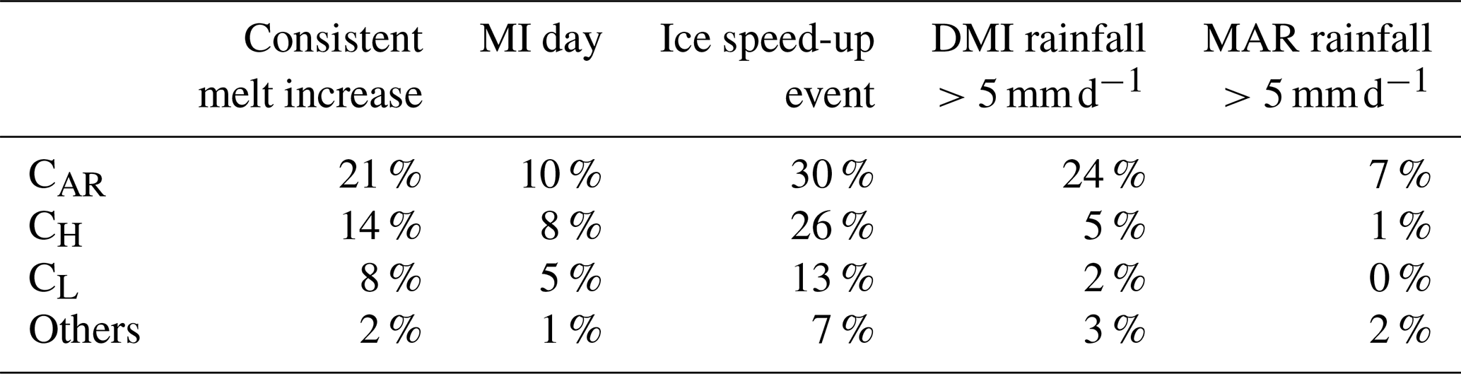
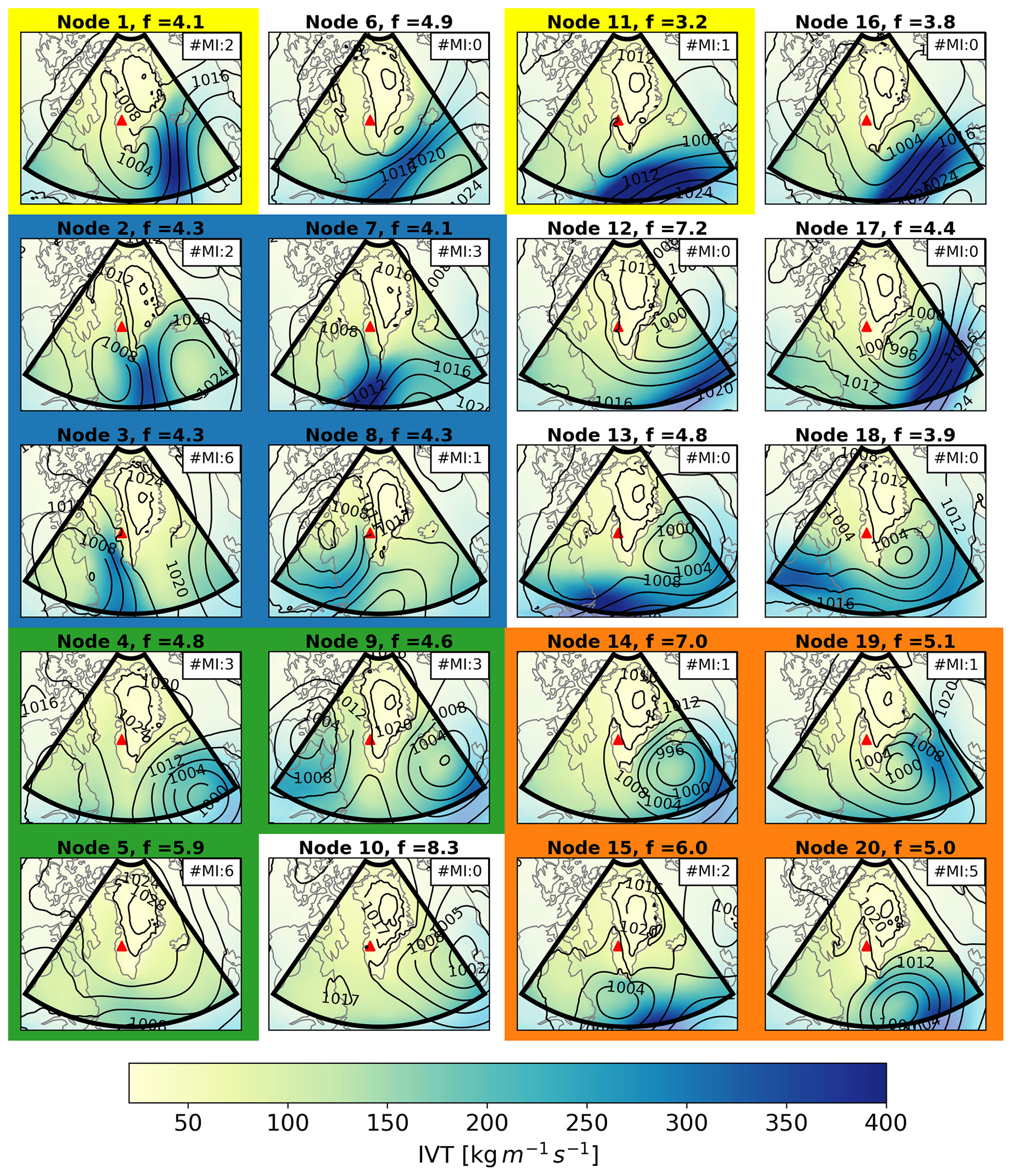
Figure 6The 4×5 SOM showing 20 characteristic patterns of IVT (colour bar) over Greenland. The thin black contours show the corresponding mean SLP field, averaged over the days belonging to the given pattern. The SOM method is applied over the domain outlined with a bold black line. The location of the Russell Glacier is indicated with a red triangle. Each SOM pattern is labelled with its frequency of occurrence f (%), calculated over the entire period: May–October, 1979–2020, and #MI indicates the number of MI days that occur during each node. Nodes with non-zero #MI are grouped into the CAR cluster (blue shading), CH cluster (green shading), and CL cluster (orange shading), while the remaining ungrouped nodes are highlighted in yellow.
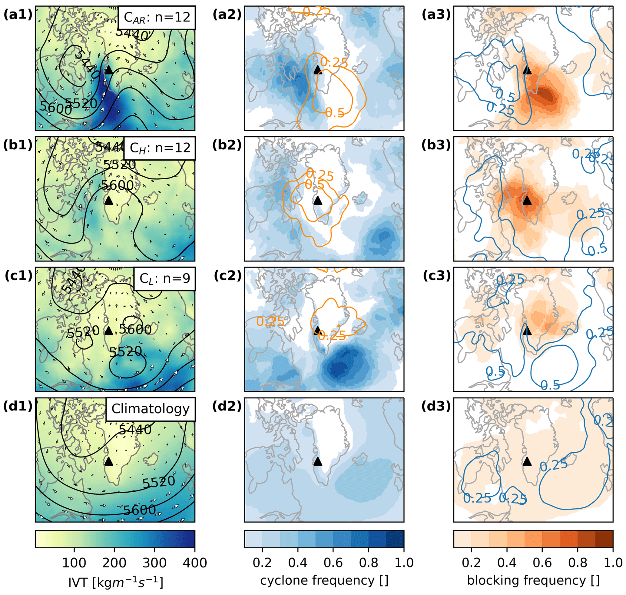
Figure 7Left column (a1, b1, c1, d1): composites of IVT (colour bar), Z500 (black contours), and mean wind at 500 hPa (arrows) for all MI days per cluster, as well as for the climatology (average over all days from May to October, 2009–2012). Middle column (a2, b2, c2, d2): the same as the left column but for composites of cyclone frequency (shaded blue) and blocking frequency (orange contours), calculated as explained in Sect. 2.4. Right column (a3, b3, c3, d3): the same as the left column but for composites of the blocking frequency (shaded orange) and cyclone frequency (blue contours). The location of the Russell Glacier is indicated with a black triangle.
4.3 Trajectory analysis
Here we show the results of the trajectory analysis, where the Lagrangian trajectory model, calculating the 5 d backward trajectories, is applied to each MI day of the three main clusters (CAR, CH, and CL). The results are presented for each cluster separately, synthesizing all the trajectories for MI days that belong to a given cluster. Figure 8 shows the trajectories arriving in the lower troposphere (at 750 hPa) over the Russell Glacier, while the results for the surface and mid-troposphere trajectories are shown in Figs. S1 and S2. Air masses arriving in the lower troposphere at around 750 hPa (Fig. 8) are able to show the development of moisture and temperature patterns that are relevant for surface melt (e.g. Tedesco et al., 2013), as highlighted by a high moisture content of up to 6 g kg−1(Fig. 8f) and the visibility of coherent trajectory patterns (Fig. 8a–c). Thus, we primarily focus on lower tropospheric (750 hPa) trajectories but additionally analyse the trajectories of (i) air masses arriving at 500 hPa (Fig. S2) to get information about higher-reaching clouds and the large-scale dynamics of the troposphere and (ii) air masses arriving at surface level (Fig. S1) to get information about the near-surface atmospheric conditions in each cluster.
The results show that CAR and CL have distinctly different air mass origins to the south and to the east of the GrIS, respectively, due to the prevalent anticyclonic and cyclonic flow regime (Fig. 8a and c). CH air masses, like those of CAR, approach the study area from the southwest but have larger spatial variability (Fig. 8b) and typically travel at higher altitudes than those of CAR and CL (Fig. 8d). CAR air parcels hold about twice as much moisture as those in CH and CL throughout the 5 d prior to arrival at the study area, which is related to their warmer origin in the south (Fig. 8e and f). In the CAR cluster, specific humidity increases along with temperature, while the air parcels reach lower altitudes of mostly below 850 hPa until 12 h prior to arrival (Fig. 8d–f). During the last 12 h, the air parcels ascend along the GrIS and expand and cool adiabatically while reaching saturation (Fig. 8d, e, g). Condensation of water vapour causes specific humidity (Q) to drop (Fig. 8f), while the air mass warms diabatically, causing further ascent and counteracting parts of the ongoing adiabatic cooling. To summarize, air parcels of the CAR cluster arriving on average with RH >90 % are likely linked to precipitation and overcast conditions and hold much more moisture than those of CH and CL (Fig. 8g). We note that these differences among the clusters are more strongly pronounced at higher altitudes than for the air mass arriving near the surface (Figs. S1 and S2).
A key characteristic of the CH air masses is their low specific and relative humidity over the considered 5 d period (Fig. 8f and g). They show little vertical motion with a tendency towards descent (Fig. 8d), more so for air mass arriving at lower levels (Fig. S1). Accordingly, these air parcels move roughly isothermally or they warm adiabatically according to their vertical displacement (Fig. 8e). Thus, despite the aforementioned similarities in the anticyclonically dominated Z500 pattern and the air mass origin of the CH and CAR clusters, CH air masses travel at higher altitudes and are drier relative to those in the CAR cluster.
While the properties of CL air parcels resemble those of CH over at least the first 3 d, they show clearly distinct signs of flowing over the GrIS. Initially moving at about a constant altitude slightly below 750 hPa, the air mass starts to ascend 2 d prior to arrival when advected towards the eastern segment of the GrIS (Fig. 8b and d). Relative humidity (RH) increases (Fig. 8g), and at least in some events, Q decreases due to condensation and precipitation (Fig. 8f). After crossing the ice divide from the east, the air masses descend along the western GrIS to the study area in a foehnlike flow, warming adiabatically and reaching low values of RH of <60 %. For near-surface air masses, this drying is even more pronounced, causing a final RH of around 50 % (Fig. S1 in the Supplement). The low RH in CL in the study region is due to the drop in Q east of the ice divide (Fig. S1d and f), which can be related to condensation of water vapour during the air mass ascent.
In summary, the trajectory analysis indicates that melt during CAR events is related to intrusions of warm–moist air masses travelling along the strongly meridional flow (Fig. 8). Air parcels approach the region of high IVT and increase in humidity near the surface, while condensation and likely precipitation dominate in the vicinity of the study area. The blocking, which centred over the Russell Glacier for most MI days in the CH cluster, leads to the air parcels being dry and descending to low altitudes as they approach the study area. The air parcels related to CL approach the study region from the east, being advected by the cyclone south of the GrIS. Their final descent follows the condensation of water vapour over the eastern GrIS and causes adiabatic warming, which results in low RH and clear-sky conditions over the study region.
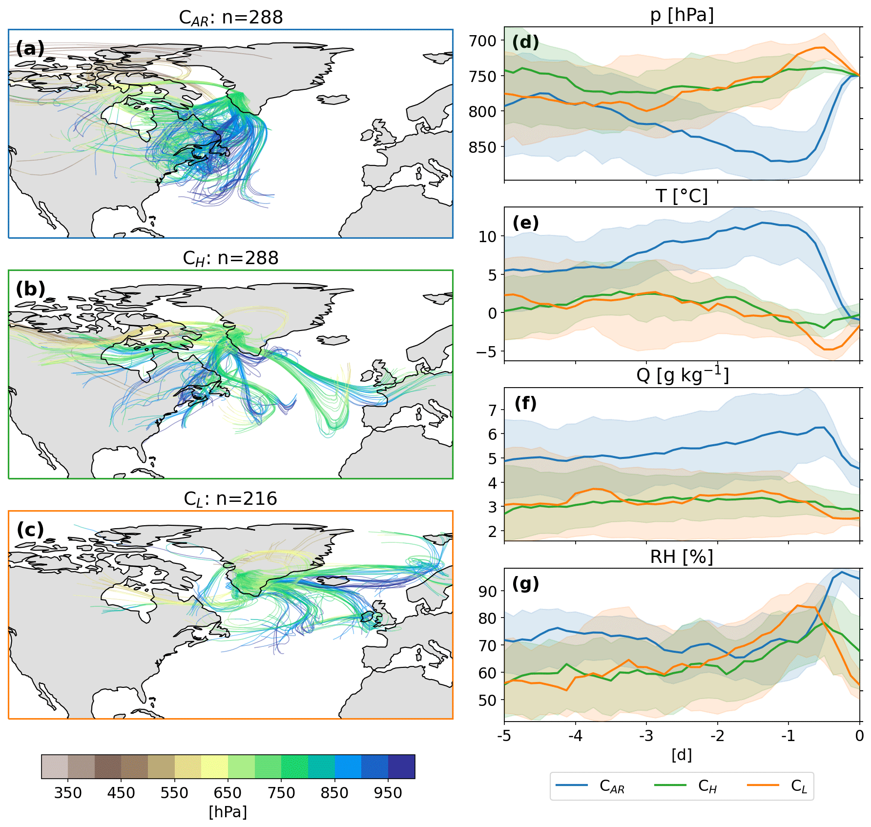
Figure 8(a–c) The 5 d backward trajectories coloured according to their vertical level for all MI days in each of the main clusters (CAR, CH, and CL). Trajectories are initiated (time =0 d) at 750 hPa at eight locations in the Russell Glacier ablation area at 09:00, 12:00, and 15:00 UTC−3. (d–g) Temporal evolution from time d (origin) to time =0 d (arrival over the Russell Glacier) of median variables (assessed as the median from the MI days belonging to the given cluster): pressure (p), temperature (T), specific humidity (Q), and relative humidity (RH), with the respective intertercile (33th–66th percentile) range shaded.
4.4 Local drivers of the melt-induced speed-ups
Here we investigate local meteorological conditions and contributors to energy available for melt during the 33 MI days linked to the three main weather patterns (CAR, CH, and CL). During the 12 MI days in the CAR cluster, when substantially moist air mass arrives in the study area, cloud cover is high with a median of 89 % from PROMICE measurements (Fig. 9e). While CH includes days with high and low cloud cover, CL has a median cloud cover of 34 % and only two events above 40 %. These differences in cloud cover are reflected in the melt energy fractions of SEB components: CH and CL both average at >100 % (101 % and 114 %) melt energy from net shortwave radiation (SWnet), while ∼25 % from the sensible heat flux (SHF) is cancelled by negative net longwave radiation, LWnet (−22 % for CH and −30 % for CL) and slightly negative latent heat flux, LHF. The particularly low cloud cover and high SWnet in CL are further evidence for a foehn clearance which is expected from the downsloping winds with low final RH as trajectories arrive over the SW GrIS (Sect. 4.3). In contrast, CAR averages at a low SWnet contribution of ∼58 % and an almost negligible LWnet (−4 %), which indicates strong downward LW radiation from clouds. In addition, SHF contributes on average 41 % of the melt energy, which is almost twice the contribution of CH and CL. However, substantial within-cluster variability remains and partly exceeds the differences among the three clusters (Fig. 9).
Despite the contrasting local drivers of the SEB, the increase in melt during the MI days is similarly distributed among the three clusters with values from 3 to 22 mm d−2. Looking at the whole duration of the speed-up event, which can be anything from 1 to 8 d, only the CAR cluster shows a substantially larger total melt increase (e.g. up to 40 mm d−1 per event). Similarly, the largest total ice velocity increases, up to 160 m yr−1, are observed in the CAR cluster, while the highest ice velocity increases of the other two clusters remain below 70 m yr−1. Local near-surface air temperatures show a similar distribution for all clusters with values between −4 and +5 ∘C, averaged over the three PROMICE stations on the Russell Glacier. Note that Ta at the lowest station (KAN L) and during daytime is always substantially higher than the spatiotemporal average of the Russell Glacier ablation area, and, thus, surface melt can occur even if averaged temperatures are below 0 ∘C.
Finally, the ice speed-up events in the CL cluster only occur in June and July, while CAR and CH events are more evenly distributed across the melt season and include two to three spring events each (Fig. 9). These spring events mark the two strongest ice speed-up events in the CH cluster and are even stronger (>90 m yr−1) in the CAR cluster. The CAR cluster also includes one spring event with anomalously low cloud cover and corresponding high SWnet and low LWnet.
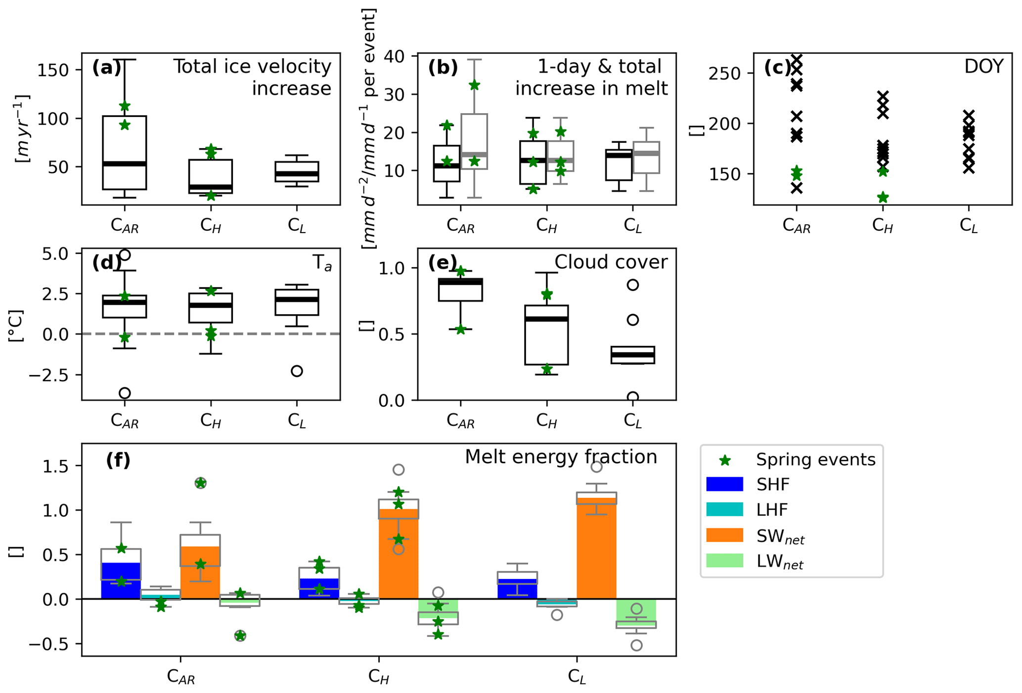
Figure 9Boxplots for each of the three main clusters (CAR, CH, and CL) for the MI days showing the (a) total ice velocity increase; (b) 1 d (black) and total melt increase (grey) for each melt-induced speed-up; (c) day of the year (DOY) (d) air temperature (Ta); (e) cloud cover; and (f) melt energy fraction of different components of SEB – sensible heat flux (SHF), latent heat flux (LHF), net shortwave radiation (SWnet), and net longwave radiation (LWnet). Melt increase data represent an average over the three melt datasets only during days where the increase is consistent among them (Sect. 3.3). Spring events are marked with green stars in each panel.
Our results complement existing research that links synoptic-scale weather systems to GrIS surface melt but with a focus on the implications for ice speed-up events rather than the surface mass balance. Given the dynamic response of GrIS to ongoing climate change, including possible changes in synoptic-scale conditions (Schuenemann and Cassano, 2010) and extreme weather events (Mattingly et al., 2023), studying the current links between the ice speed-up events and synoptic-scale weather conditions is a necessary starting point towards improved projections. Both blocking and ARs have been shown to increase the melt of GrIS (Fettweis et al., 2013; Delhasse et al., 2018; Huai et al., 2020; Bonne et al., 2015; Mattingly et al., 2018). Here we showed that both of these systems are also critical for driving the ice speed-ups at the Russell Glacier through rapid increases in melt, with anomalously high blocking frequencies for both CAR and CH clusters of weather patterns and a strong AR-like southerly IVT band in CAR.
For the 36 analysed MI days, the occurrence and the location of blocking and cyclones drive the local weather conditions in southwest Greenland (Fig. 7). While cyclonic conditions over the Labrador Sea and Baffin Bay in the CAR cluster lead to warm–moist air advection towards the SW GrIS, a cyclone southeast of Greenland (CL cluster) is associated with dry conditions at the SW GrIS due to a foehnlike easterly air advection over the ice sheet. A similar foehnlike flow has been observed and linked to increased melting in northeast Greenland (Mattingly et al., 2020, 2023) and the Antarctic Peninsula (Turton et al., 2018; Laffin et al., 2021). As observed in the CL cluster, reduced cloud cover, increased SWnet, and high temperatures contribute to increased melting in downsloping foehn flow (Hahn et al., 2020; Mattingly et al., 2020). Our analysis of local meteorological conditions during CL (Fig. 9f) does not suggest particularly strong turbulent heat fluxes, which have previously been linked to foehn winds (Elvidge et al., 2020). While beyond the scope of this study, a Lagrangian analysis of foehn and its interaction with katabatic winds in the atmospheric boundary layer in southern Greenland could be a scope of future research.
Similarly, our results highlight the importance of the exact location of a blocking system for local surface energy fluxes, which corroborates previous studies (Ward et al., 2020; Preece et al., 2022). While the CAR cluster typically shows advection of moist air with the highest blocking frequencies in southeast Greenland, a blocking system centred over southwest Greenland (CH cluster) is associated with drier conditions and descending air masses. The difference in humidity among the synoptic patterns is especially pronounced in our analysis as the clustering is based on the IVT fields. Nevertheless, the strong contrast between CAR and CH highlights thermodynamical differences between blocking systems in southwest and southeast Greenland. In particular, when the blocking is located southeast of Greenland (CAR; Fig. 7a3), air masses are forced to ascend over the SW GrIS, which leads to condensation (Hermann et al., 2020) and, thus, cloudy conditions that impact the local SEB.
Positive anomalies in incoming longwave (LW) radiation and sensible heat flux (SHF), relative to the climatology over the observational period, dominate in the CAR cluster, which is in line with the findings of Mattingly et al. (2020) that turbulent heat fluxes, particularly SHF, dominate the melt energy during strong AR events, while net LW and net shortwave (SW) radiation largely cancel each other out. The relative impact of incoming SW and LW radiation depends on surface albedo and cloud properties (Hofer et al., 2019). As the investigated area of the Russell Glacier is predominantly in the ablation zone, the net SW radiation is expected to dominate due to lower albedo of bare ice, and cloud cover typically reduces surface melt (Wang et al., 2019). We observe this effect with SWnet as the dominant SEB component in CH and CL clusters (Fig. 9), but due to the strong SHF in CAR, absolute daily melt increases (Fig. 9b) are similar among all three clusters. However, a key difference among the clusters is that only during CAR events are multi-day melt increases of up to 40 mm d−1 per event common. Prominent among these multi-day melt increases are two events during July 2012, which are widely discussed in the literature (e.g. Nghiem et al., 2012; Neff et al., 2014; Bonne et al., 2015; Fausto et al., 2016b). The extreme melt is caused by ARs that enhance incoming LW radiation due to cloudy conditions and SHF due to enhanced near-surface wind speed and exceptionally warm temperatures. The two melt episodes in July 2012 lead to two of the four strongest ice speed-up events on the Russell Glacier with velocity increases of 99 and 160 m yr−1 during 3 and 4 d, respectively. Notably, both events have occurred during consecutive days within the CAR cluster (specifically node 3 in the SOM, Fig. 6) and with the highest IVT values in southwest Greenland.
We show that the AR-like IVT bands in CAR and particularly in SOM node 3 can often, but not always, lead to extreme melting and ice speed-ups. Specifically, 21 % of days that belong to the CAR cluster lead to a consistent melt increase and 30 % of days overlap with the ice speed-up event (Table 1). In comparison, days that belong to the CH and CL clusters show smaller conditional probabilities (Table 1). Within CAR, conditional probabilities of a melt increase and an ice speed-up event are particularly high for SOM node 3 with 30 % and 43 %, respectively. The strong IVT for the 12 ice speed-ups within CAR (Fig. 7a1) compared to average IVT values in the CAR cluster (Fig. 6; nodes 2, 3, 7, 8) indicates that CAR events not leading to extreme melting and ice speed-up events are likely associated with weaker ARs. This finding is consistent with the previously identified relationship between AR intensity and melt in Greenland (Mattingly et al., 2020). Furthermore, the generally low conditional probabilities (Table 1) indicate the importance of other factors in addition to the synoptic forcing, such as local conditions in the boundary layer and the evolution of the subglacial drainage system, pointing towards an interesting direction for further research.
As expected from the high IVT values, CAR is also linked to the highest rainfall (Table 1), which can further increase the water supply to the glacier bed. In addition, rain heat flux can provide additional melt energy, which is not considered in this study. While the rain heat flux is negligible on seasonal timescales (Charalampidis et al., 2015), it can be a non-negligible contributing factor for individual melt events. Doyle et al. (2015) found a relative contribution of rain heat flux of 0.5 % during a rainfall event in 2011, and Fausto et al. (2016a) estimated a 7 % contribution during two extreme melt episodes in July 2012. Of the 10 ice speed-up events with a substantial (>5 mm d−2) daily increase in rainfall in either RDMI or RMAR datasets, 6 occur during CAR. Note that in contrast to melt, daily increases in rainfall (in mm d−2) mostly correspond to the total rainfall per day as the increase in rainfall is derived from the initial value of 0 mm d−1. All 10 ice speed-up events with >5 mm d−2 daily increase in rainfall co-occur with a consistent melt increase and are part of the melt speed-ups. Only in one case (27 August 2010) is rainfall clearly dominating, with both datasets agreeing on a larger daily increase in rainfall than surface melt (Table S1 in the Supplement).
Considering the nine non-melt speed-ups, five are of small amplitude (<25 m yr−1) and may be caused by a slight increase in surface melt, which was not consistently measured in all three datasets. Of the four remaining non-melt speed-ups, the only spring event on 18 May 2009 is likely related to a melt increase from 2 d before, which is above the maximum lag considered in our identification method (Sect. 3.3). Further, two non-melt events in late July 2009 co-occurred with multiple large lake drainages, all of which occurred at >1200 m elevation. Thus, the lake drainage events are likely to have caused the ice acceleration at the high-elevation sites L4–L6, which dominate the increase in mean ice velocities for both events. The strongest non-melt speed-up on 2 July 2009 is seemingly unexplained with no observed rapid lake drainage event or significant increase in melt or rainfall. However, Bartholomew et al. (2011b) identified rapid lake drainages within the hydrological catchment of the glacier (and within the spatial domain in Fig. 1) as a likely cause of the observed pulse in glacial water discharge, which can also explain the ice speed-up event. This highlights (i) the possibility that the method we used for lake identification and drainage may not identify all rapid lake drainage events due to variable cloud cover between different satellite imagery products used and (ii) differences in criteria that different studies used for identifying rapid drainage events. Given the limitations associated with image resolution, methodological sensitivity, variable cloud cover, and satellite return frequency, as well as the localized nature of lake drainage events, a quantitative comparison between the influence of surface melt and lake drainages on ice speed-up events remains challenging. Qualitatively, we observe that most (14 out of 16) ice speed-up events that co-occur with lake drainages also coincide with melt increases. While lake drainage areas and melt increase values (Table S1) give an indication of their relative importance for each ice speed-up event, a quantitative attribution is not within the scope of this paper.
As this study is largely based on data from local measurement stations, it is subject to common uncertainties associated with observations in remote locations. In particular, there are some gaps in the observed time series due to power failure (Sect. 2). We minimized these uncertainties by using multiple different datasets, in particular for the estimates of surface melt. In contrast, rainfall measurements are sparse on the GrIS, and rainfall data for the Russell Glacier are only based on one off-glacier measurement station (Sect. 2.2) and simulations from the regional climate model. Accordingly, absolute rainfall values are subject to large uncertainty, but nevertheless the data indicate that rainfall is negligible compared to surface melt for most ice speed-up events. Only during four events is the maximum daily increase in any of the rainfall datasets larger than the melt increase, despite the overestimation of RDMI due to the low elevation of the station (Sect. 2.2). In addition to measurement uncertainties, there is also some subjectivity in methodological choices such as the definition and identification of ice speed-up events and the clustering of the three main patterns (CAR, CH, and CL) within the SOM. Sensitivities of the results to these choices are described in Sect. 3.2 for the speed-up event definition and in Schmid (2021) for the clustering within SOMs.
Despite the mentioned uncertainties, this study provides insights into atmospheric drivers of melt-induced ice speed-up events on the Russell Glacier, where Bartholomew et al. (2012) found that the seasonal ice velocity signal is dominated by short-term ice speed-up events. As the frequency and intensity of the synoptic patterns, linked to the melt-induced speed-ups, may change in the warming climate (Schuenemann and Cassano, 2010), so can the future of speed-up events. In particular, a 30 % conditional probability (Table 1) and high amplitudes of up to 160 m yr−1 (Fig. 9) for ice speed-up events under CAR indicate their sensitivity to ARs, which show an increasing trend in observations between 1979 and 2015 (Mattingly et al., 2016). A possible extension of this study would be to quantify the influence of synoptically forced ice speed-ups on annual mean ice velocities and to assess the impact of climate warming on these events. An explicit consideration of the dynamical subglacial drainage system, e.g. through modelling (Koziol and Arnold, 2018) and through detailed analysis of winter ice velocities that may offset enhanced summer velocities (Tedstone et al., 2013; Sole et al., 2013), can help constrain uncertainties in future studies. While the Russell Glacier is representative of a large part of the GrIS margin (Sect. 1; Shepherd et al., 2009), more high-resolution ice velocity measurements and a similar analysis performed for different glaciers in Greenland are required to assess ice-sheet-wide effects.
This study analysed atmospheric drivers of melt-induced ice speed-up events at the Russell Glacier in southwest Greenland. These short-term speed-up events were identified from daily velocity time series collected from six GPS stations along the glacier for each summer (May–October) over the 2009–2012 period. In total, 45 ice speed-up events were identified, of which 36 are considered melt-induced events, each spanning a duration from 1 to 4 d of consistently increasing melt. The melt is calculated from three different datasets: two in situ observational datasets and one regional climate model forced by ERA5 reanalysis. Characteristic patterns of integrated water vapour transport (IVT), assessed over a large domain covering Greenland, were identified according to the self-organizing map (SOM) algorithm. Each melt-induced speed-up event was then linked to one of the characteristic IVT patterns from the SOM, and 5 d backward trajectories, tracking the air mass movement, were analysed for each of these events.
Our results indicate that a short-term increase in surface melt is the dominant driver of the speed-up events in the observational period, rather than the rainfall or lake drainage events. Daily increases in rainfall are larger than in meltwater only during four ice speed-up events, despite considering the maximum of two rainfall datasets available for the study area. In agreement with previous studies, we find the largest influence of meltwater on ice accelerations in the beginning of each melt season (May). Following initial increases in surface melt, the lower-elevation GPS sites along the glacier record ice velocity increases of up to 311 m yr−1 per event (112 m yr−1, when averaged over all GPS sites), which was the strongest overall ice acceleration over the observational period. In addition, only two of the non-melt speed-up events are linked to lake drainages identified within the same observational period.
We found that the characteristic weather patterns that are linked to the melt-induced speed-ups can be grouped into three main clusters: patterns that resemble atmospheric rivers with a landfall at southwest Greenland (labelled CAR cluster), anticyclonic blocking centred over southwest Greenland (CH cluster), and low-pressure systems centred either south or southeast of Greenland (CL cluster). In all three clusters, above-average blocking frequencies over Greenland are observed but with varying location and intensity, leading to different air advections and local conditions on the Russell Glacier. Despite experiencing only minor shifts in the position of weather systems, e.g. of the upper-level block in CAR and CH, the local surface energy budget can differ substantially. These differences are largely explained by contrasting air mass origins and evolution prior to their arrival in southwest Greenland:
-
Weather patterns in the CAR cluster are characterized by advection of warm and humid air within a narrow AR-like band from the south onto the study region, forced by a cyclone over the Labrador Sea and a blocking anticyclone at the southern tip of Greenland. The energy available for melt is mainly supplied by anomalously high sensible heat flux and incoming longwave radiation. The trajectory analysis reveals that the system originates predominately off the east coast of the United States, containing particularly high humidity in the mid-troposphere rather than near the surface.
-
Weather systems within the CH cluster show typical blocking conditions, centred over southwest Greenland, where surface melt is mainly driven by strong incoming shortwave radiation. The trajectory analysis reveals a few anticyclonically descending airstreams and generally dry air being advected from the southeast to the southwest of Greenland.
-
Weather patterns in the CL cluster, occurring only in June and July, display a cyclone south to southeast of Greenland. Similar to foehn wind phenomena, the flux of the air from the east to the west over the ice sheet brings warm and clear-sky conditions to the study area, driving the increase in surface melt.
A key conclusion from the analysis is that the strongest ice speed-up events occur either during spring events or during atmospheric river events. Spring events mark the first surface–bed connection in the lower regions of the glacier, where water flows into a distributed subglacial drainage system, which causes strong accelerations. Contrastingly, warm-air advection in the CAR events can lead to strong ice speed-up events by causing multiple (2 to 3) days of continuously increasing surface melt, which can overload even an efficient (channelized) subglacial drainage system in summer. As these weather patterns may change in frequency and intensity with the warming climate, so may the frequency and intensity of ice speed-up events, ultimately altering the mass loss of the ice sheet. While the implications can be substantial for the future of Greenland and global sea level rise, the current availability of long-term velocity measurements in Greenland is relatively limited. More in situ and remote sensing velocity data, as well as data on lake drainage events, are needed to validate our results, investigate GrIS-wide effects, and constrain uncertainties in future projections.
The PROMICE station data are available at https://doi.org/10.22008/FK2/8SS7EW (Fausto et al., 2022), the IMAU data in the supplement of van de Wal et al. (2015), the UK PDC data at https://doi.org/10.5285/1f69fba3-4c62-47ad-8119-08cfeec05e46 (Tedstone and Nienow, 2018), and the DMI data at https://www.dmi.dk/fileadmin/user_upload/Rapporter/TR/2020/DMIRep20-08_old_dataformat_1958_2013.zip (Cappelen, 2020). MAR is available at https://doi.org/10.18739/A28G8FJ7F (Fettweis, 2022) and model outputs may be requested from Xavier Fettweis (xavier.fettweis@uliege.be). Finally, ERA5 data are available at https://doi.org/10.24381/cds.adbb2d47 (Hersbach et al., 2023). Scripts used for the analyses and plotting, mostly written in Python 3.9, are available on request from the authors.
The supplement related to this article is available online at: https://doi.org/10.5194/tc-17-3933-2023-supplement.
TS conducted the analysis with supervision from VR. MH calculated and visualized trajectories, provided feedback, and supported the writing of the paper. AT supported the analysis and interpretation of the ice velocity and lake drainage observations. JML and SB provided the lake drainage data. TS wrote the paper with comments from all co-authors.
The contact author has declared that none of the authors has any competing interests.
Publisher's note: Copernicus Publications remains neutral with regard to jurisdictional claims in published maps and institutional affiliations.
We would like to express our great appreciation to Heini Wernli and Daniel Farinotti for providing feedback and support during Timo Schmid's MSc thesis, on which this paper is based. Further, we extend our thanks to the Zeno Karl Schindler Foundation for supporting the MSc thesis with a grant. We also thank Jennifer Walker, who previously worked on a related project, for providing a detailed explanation of the work she had done and the datasets she used. Data from the Programme for Monitoring of the Greenland Ice Sheet (PROMICE) and the Greenland Analogue Project (GAP) were provided by the Geological Survey of Denmark and Greenland (GEUS) at http://www.promice.dk (last access: 12 September 2023). Further, we acknowledge the Danish Meteorological Institute for providing meteorological station observations, and we thank Xavier Fettweis for distributing MAR output data.
This research has been supported by the Natural Sciences and Engineering Research Council (NSERC) of Canada (Discovery Grant to Valentina Radić).
This paper was edited by Kristin Poinar and reviewed by two anonymous referees.
Alduchov, O. A. and Eskridge, R. E.: Improved Magnus Form Approximation of Saturation Vapor Pressure, J. Appl. Meteorol. and Climatology, 35, 601–609, https://doi.org/10.1175/1520-0450(1996)035<0601:IMFAOS>2.0.CO;2, 1996. a
Ashmore, D. W., Mair, D. W. F., Higham, J. E., Brough, S., Lea, J. M., and Nias, I. J.: Proper orthogonal decomposition of ice velocity identifies drivers of flow variability at Sermeq Kujalleq (Jakobshavn Isbræ), The Cryosphere, 16, 219–236, https://doi.org/10.5194/tc-16-219-2022, 2022. a
Barnes, E. A. and Screen, J. A.: The impact of Arctic warming on the midlatitude jet-stream: Can it? Has it? Will it?, Wires. Clim. Change, 6, 277–286, https://doi.org/10.1002/wcc.337, 2015. a
Bartholomew, I., Nienow, P., Mair, D., Hubbard, A., King, M. A., and Sole, A.: Seasonal evolution of subglacial drainage and acceleration in a Greenland outlet glacier, Nature Geosci., 3, 408–411, https://doi.org/10.1038/ngeo863, 2010. a, b
Bartholomew, I., Nienow, P., Sole, A., Mair, D., Cowton, T., King, M., and Palmer, S.: Seasonal variations in Greenland Ice Sheet motion: Inland extent and behaviour at higher elevations, Earth Planet. Sc. Lett., 307, 271–278, https://doi.org/10.1016/j.epsl.2011.04.014, 2011a. a, b, c, d, e, f
Bartholomew, I., Nienow, P., Sole, A., Mair, D., Cowton, T., Palmer, S., and Wadham, J.: Supraglacial forcing of subglacial drainage in the ablation zone of the Greenland ice sheet, Geophys. Res. Lett., 38, L08502, https://doi.org/10.1029/2011GL047063, 2011b. a
Bartholomew, I., Nienow, P., Sole, A., Mair, D., Cowton, T., and King, M. A.: Short-term variability in Greenland Ice Sheet motion forced by time-varying meltwater drainage, J. Geophys. Res.-Earth., 117, F03002, https://doi.org/10.1029/2011JF002220, 2012. a, b, c, d
Bonne, J., Steen-Larsen, H. C., Risi, C., Werner, M., Sodemann, H., Lacour, J.-L., Fettweis, X., Cesana, G., Delmotte, M., Cattani, O., Vallelonga, P., Kjaer, H. A., Clerbaux, C., Sveinbjörnsdóttir, A. E., and Masson-Delmotte, V.: The summer 2012 Greenland heat wave: In situ and remote sensing observations of water vapor isotopic composition during an atmospheric river event, J. Geophys. Res.-Atmos., 120, 2970–2989, https://doi.org/10.1002/2014jd022602, 2015. a, b
Brayshaw, D. J., Hoskins, B., and Blackburn, M.: The basic ingredients of the North Atlantic storm track. Part I: Land–sea contrast and orography, J. Atmos. Sci., 66, 2539–2558, https://doi.org/10.1175/2009JAS3078.1, 2009. a
Cappelen, J.: Weather observations from Greenland 1958–2019, Technical Report 20-08, Danish Meteorological Institute, Copenhagen, http://www.dmi.dk/laer-om/generelt/dmi-publikationer (last access: 12 September 2023), 2020. a, b
Chandler, D. M., Wadham, J. L., Lis, G. P., Cowton, T., Sole, A., Bartholomew, I., Telling, J., Nienow, P., Bagshaw, E. B., Mair, D., Vinen, S., and Hubbard, A.: Evolution of the subglacial drainage system beneath the Greenland Ice Sheet revealed by tracers, Nature Geosci., 6, 195–198, 2013. a, b
Charalampidis, C., van As, D., Box, J. E., van den Broeke, M. R., Colgan, W. T., Doyle, S. H., Hubbard, A. L., MacFerrin, M., Machguth, H., and Smeets, C. J. P. P.: Changing surface–atmosphere energy exchange and refreezing capacity of the lower accumulation area, West Greenland, The Cryosphere, 9, 2163–2181, https://doi.org/10.5194/tc-9-2163-2015, 2015. a
Chen, L., Johannessen, O. M., Wang, H., and Ohmura, A.: Accumulation over the Greenland Ice Sheet as represented in reanalysis data, Adv. Atmos. Sci., 28, 1030–1038, https://doi.org/10.1007/s00376-010-0150-9, 2011. a
Chu, V. W.: Greenland ice sheet hydrology, Prog. Phys. Geog., 38, 19–54, https://doi.org/10.1177/0309133313507075, 2014. a, b
Clason, C. C., Mair, D. W. F., Nienow, P. W., Bartholomew, I. D., Sole, A., Palmer, S., and Schwanghart, W.: Modelling the transfer of supraglacial meltwater to the bed of Leverett Glacier, Southwest Greenland, The Cryosphere, 9, 123–138, https://doi.org/10.5194/tc-9-123-2015, 2015. a
Cooley, S. W. and Christoffersen, P.: Observation Bias Correction Reveals More Rapidly Draining Lakes on the Greenland Ice Sheet: Bias in Rapid Lake Drainage Detections, J. Geophys. Res.-Earth., 122, 1867–1881, https://doi.org/10.1002/2017JF004255, 2017. a
Croci-Maspoli, M., Schwierz, C., and Davies, H. C.: A Multifaceted Climatology of Atmospheric Blocking and Its Recent Linear Trend, J. Climate, 20, 633–649, https://doi.org/10.1175/JCLI4029.1, 2007. a
Dacre, H. F., Clark, P. A., Martinez-Alvarado, O., Stringer, M. A., and Lavers, D. A.: How Do Atmospheric Rivers Form?, B. Am. Meteorol. Soc., 96, 1243–1255, https://doi.org/10.1175/BAMS-D-14-00031.1, 2015. a
Delhasse, A., Fettweis, X., Kittel, C., Amory, C., and Agosta, C.: Brief communication: Impact of the recent atmospheric circulation change in summer on the future surface mass balance of the Greenland Ice Sheet, The Cryosphere, 12, 3409–3418, https://doi.org/10.5194/tc-12-3409-2018, 2018. a, b
Delhasse, A., Kittel, C., Amory, C., Hofer, S., van As, D., Fausto, S. R., and Fettweis, X.: Brief communication: Evaluation of the near-surface climate in ERA5 over the Greenland Ice Sheet, The Cryosphere, 14, 957–965, https://doi.org/10.5194/tc-14-957-2020, 2020. a
Doyle, S. H., Hubbard, A., van de Wal, R. S. W., Box, J. E., van As, D., Scharrer, K., Meierbachtol, T. W., Smeets, P. C. J. P., Harper, J. T., Johansson, E., Mottram, R. H., Mikkelsen, A. B., Wilhelms, F., Patton, H., Christoffersen, P., and Hubbard, B.: Amplified melt and flow of the Greenland ice sheet driven by late-summer cyclonic rainfall, Nature Geosci., 8, 647–653, https://doi.org/10.1038/ngeo2482, 2015. a, b
Dyer, A. J.: A review of flux-profile relationships, Bound.-Lay. Meteorol., 7, 363–372, https://doi.org/10.1007/BF00240838, 1974. a
Elvidge, A. D. and Renfrew, I. A.: The Causes of Foehn Warming in the Lee of Mountains, B. Am. Meteorol. Soc., 97, 455–466, https://doi.org/10.1175/BAMS-D-14-00194.1, 2016. a
Elvidge, A. D., Kuipers Munneke, P., King, J. C., Renfrew, I. A., and Gilbert, E.: Atmospheric Drivers of Melt on Larsen C Ice Shelf: Surface Energy Budget Regimes and the Impact of Foehn, J. Geophys. Res.-Atmos., 125, e2020JD032463, https://doi.org/10.1029/2020JD032463, 2020. a
Fausto, R. S., van As, D., Box, J. E., Colgan, W., and Langen, P. L.: Quantifying the Surface Energy Fluxes in South Greenland during the 2012 High Melt Episodes Using In-situ Observations, Front. Earth Sci., 4, 82, https://doi.org/10.3389/feart.2016.00082, 2016a. a
Fausto, R. S., van As, D., Box, J. E., Colgan, W., Langen, P. L., and Mottram, R. H.: The implication of nonradiative energy fluxes dominating Greenland ice sheet exceptional ablation area surface melt in 2012, Geophys. Res. Lett., 43, 2649–2658, https://doi.org/10.1002/2016GL067720, 2016b. a
Fausto, R. S., van As, D., Mankoff, K. D., Vandecrux, B., Citterio, M., Ahlstrøm, A. P., Andersen, S. B., Colgan, W., Karlsson, N. B., Kjeldsen, K. K., Korsgaard, N. J., Larsen, S. H., Nielsen, S., Pedersen, A. Ø., Shields, C. L., Solgaard, A. M., and Box, J. E.: Programme for Monitoring of the Greenland Ice Sheet (PROMICE) automatic weather station data, Earth Syst. Sci. Data, 13, 3819–3845, https://doi.org/10.5194/essd-13-3819-2021, 2021. a, b
Fausto, R. S., Van As, D., and Mankoff, K. D.: AWS one boom tripod Edition 3 (deprecated), V2, GEUS Dataverse [data set], https://doi.org/10.22008/FK2/8SS7EW, 2022. a, b
Fettweis, X.: Reconstruction of the 1979–2006 Greenland ice sheet surface mass balance using the regional climate model MAR, The Cryosphere, 1, 21–40, https://doi.org/10.5194/tc-1-21-2007, 2007. a
Fettweis, X.: Modèle Atmosphérique Régional (MAR) version 3.11 regional climate model output, 1979–2019, Greenland domain, 10 kilometer (km) horizontal resolution, Arctic Data Center [data set], https://doi.org/10.18739/A28G8FJ7F (last access: 12 September 2023), 2022. a
Fettweis, X., Hanna, E., Lang, C., Belleflamme, A., Erpicum, M., and Gallée, H.: Brief communication “Important role of the mid-tropospheric atmospheric circulation in the recent surface melt increase over the Greenland ice sheet”, The Cryosphere, 7, 241–248, https://doi.org/10.5194/tc-7-241-2013, 2013. a, b
Fettweis, X., Box, J. E., Agosta, C., Amory, C., Kittel, C., Lang, C., van As, D., Machguth, H., and Gallée, H.: Reconstructions of the 1900–2015 Greenland ice sheet surface mass balance using the regional climate MAR model, The Cryosphere, 11, 1015–1033, https://doi.org/10.5194/tc-11-1015-2017, 2017. a, b
Fitzpatrick, A. A., Hubbard, A., Joughin, I., Quincey, D. J., As, D. V., Mikkelsen, A. P., Doyle, S. H., Hasholt, B., and Jones, G. A.: Ice flow dynamics and surface meltwater flux at a land-terminating sector of the Greenland ice sheet, J. Glaciol., 59, 687–696, https://doi.org/10.3189/2013JoG12J143, 2013. a
Francis, J. A. and Vavrus, S. J.: Evidence linking Arctic amplification to extreme weather in mid-latitudes, Geophys. Res. Lett., 39, L06801, https://doi.org/10.1029/2012GL051000, 2012. a
Gallé, H. and Schayes, G.: Development of a Three-Dimensional Meso-γ Primitive Equation Model: Katabatic Winds Simulation in the Area of Terra Nova Bay, Antarctica, Mon. Weather Rev., 122, 671–685, 1994. a
Gallée, H. and Duynkerke, P. G.: Air-snow interactions and the surface energy and mass balance over the melting zone of west Greenland during the Greenland Ice Margin Experiment, J. Geophys. Res.-Atmos., 102, 13813–13824, https://doi.org/10.1029/96JD03358, 1997. a
Goelzer, H., Nowicki, S., Payne, A., Larour, E., Seroussi, H., Lipscomb, W. H., Gregory, J., Abe-Ouchi, A., Shepherd, A., Simon, E., Agosta, C., Alexander, P., Aschwanden, A., Barthel, A., Calov, R., Chambers, C., Choi, Y., Cuzzone, J., Dumas, C., Edwards, T., Felikson, D., Fettweis, X., Golledge, N. R., Greve, R., Humbert, A., Huybrechts, P., Le clec'h, S., Lee, V., Leguy, G., Little, C., Lowry, D. P., Morlighem, M., Nias, I., Quiquet, A., Rückamp, M., Schlegel, N.-J., Slater, D. A., Smith, R. S., Straneo, F., Tarasov, L., van de Wal, R., and van den Broeke, M.: The future sea-level contribution of the Greenland ice sheet: a multi-model ensemble study of ISMIP6, The Cryosphere, 14, 3071–3096, https://doi.org/10.5194/tc-14-3071-2020, 2020. a
Hahn, L. C., Storelvmo, T., Hofer, S., Parfitt, R., and Ummenhofer, C. C.: Importance of Orography for Greenland Cloud and Melt Response to Atmospheric Blocking, J. Climate, 33, 4187–4206, https://doi.org/10.1175/JCLI-D-19-0527.1, 2020. a
Hanna, E.: Runoff and mass balance of the Greenland ice sheet: 1958–2003, J. Geophys. Res., 110, D13108, https://doi.org/10.1029/2004JD005641, 2005. a
Hay, J. E. and Fitzharris, B. B.: A Comparison of the Energy-Balance and Bulk-aerodynamic Approaches for Estimating Glacier Melt, J. Glaciol., 34, 145–153, https://doi.org/10.3189/S0022143000032172, 1988. a
Hermann, M., Papritz, L., and Wernli, H.: A Lagrangian analysis of the dynamical and thermodynamic drivers of large-scale Greenland melt events during 1979–2017, Weather Clim. Dynam., 1, 497–518, https://doi.org/10.5194/wcd-1-497-2020, 2020. a, b, c
Hersbach, H., Bell, B., Berrisford, P., Hirahara, S., Horányi, A., Muñoz Sabater, J., Nicolas, J., Peubey, C., Radu, R., Schepers, D., Simmons, A., Soci, C., Abdalla, S., Abellan, X., Balsamo, G., Bechtold, P., Biavati, G., Bidlot, J., Bonavita, M., De Chiara, G., Dahlgren, P., Dee, D., Diamantakis, M., Dragani, R., Flemming, J., Forbes, R., Fuentes, M., Geer, A., Haimberger, L., Healy, S., Hogan, R. J., Hólm, E., Janisková, M., Keeley, S., Laloyaux, P., Lopez, P., Lupu, C., Radnoti, G., de Rosnay, P., Rozum, I., Vamborg, F., Villaume, S., and Tépaut, J.-N.: The ERA5 global reanalysis, Q. J. Roy. Meteor. Soc., 146, 1999–2049, https://doi.org/10.1002/qj.3803, 2020. a, b
Hersbach, H., Bell, B., Berrisford, P., Biavati, G., Horányi, A., Muñoz Sabater, J., Nicolas, J., Peubey, C., Radu, R., Rozum, I., Schepers, D., Simmons, A., Soci, C., Dee, D., and Thépaut, J.-N.: ERA5 hourly data on single levels from 1940 to present, Copernicus Climate Change Service (C3S) Climate Data Store (CDS) [data set], https://doi.org/10.24381/cds.adbb2d47 (last access: 12 September 2023), 2023. a, b
Hofer, S., Tedstone, A. J., Fettweis, X., and Bamber, J. L.: Decreasing cloud cover drives the recent mass loss on the Greenland Ice Sheet, Sci. Adv., 3, e1700584, https://doi.org/10.1126/sciadv.1700584, 2017. a
Hofer, S., Tedstone, A. J., Fettweis, X., and Bamber, J. L.: Cloud microphysics and circulation anomalies control differences in future Greenland melt, Nat. Clim. Change, 9, 523–528, https://doi.org/10.1038/s41558-019-0507-8, 2019. a
Hoffman, M. J., Catania, G. A., Neumann, T. A., Andrews, L. C., and Rumrill, J. A.: Links between acceleration, melting, and supraglacial lake drainage of the western Greenland Ice Sheet, J. Geophys. Res., 116, F04035, https://doi.org/10.1029/2010JF001934, 2011. a
Holtslag, A. A. M. and De Bruin, H. A. R.: Applied Modeling of the Nighttime Surface Energy Balance over Land, J. Appl. Meteorol., 27, 689–704, https://doi.org/10.1175/1520-0450(1988)027<0689:AMOTNS>2.0.CO;2, 1988. a
Howat, I. M., Negrete, A., and Smith, B. E.: The Greenland Ice Mapping Project (GIMP) land classification and surface elevation data sets, The Cryosphere, 8, 1509–1518, https://doi.org/10.5194/tc-8-1509-2014, 2014. a
Huai, B., van den Broeke, M. R., and Reijmer, C. H.: Long-term surface energy balance of the western Greenland Ice Sheet and the role of large-scale circulation variability, The Cryosphere, 14, 4181–4199, https://doi.org/10.5194/tc-14-4181-2020, 2020. a
Kjeldsen, K., Korsgaard, N., Bjørk, A., Khan, S., Box, J., Funder, S., Larsen, N., Bamber, J., Colgan, W., van den Broeke, M., Siggaard-Andersen, M.-L., Nuth, C., Schomacker, A., Andresen, C., Willerslev, E., and Kjaer, K.: Spatial and temporal distribution of mass loss from the Greenland Ice Sheet since AD 1900, Nature, 528, 396–400, https://doi.org/10.1038/nature16183, 2015. a
Kohonen, T.: Essentials of the self-organizing map, Neural Networks, 37, 52–65, https://doi.org/10.1016/j.neunet.2012.09.018, 2013. a
Koziol, C. P. and Arnold, N.: Modelling seasonal meltwater forcing of the velocity of land-terminating margins of the Greenland Ice Sheet, The Cryosphere, 12, 971–991, https://doi.org/10.5194/tc-12-971-2018, 2018. a
Laffin, M. K., Zender, C. S., Singh, S., Van Wessem, J. M., Smeets, C. J. P. P., and Reijmer, C. H.: Climatology and Evolution of the Antarctic Peninsula Föhn Wind-Induced Melt Regime From 1979–2018, J. Geophys. Res.-Atmospheres, 126, https://doi.org/10.1029/2020JD033682, 2021. a
Lavers, D. A., Ralph, F. M., Waliser, D. E., Gershunov, A., and Dettinger, M. D.: Climate change intensification of horizontal water vapor transport in CMIP5, Geophys. Res. Lett., 42, 5617–5625, 2015. a
Le clec'h, S., Charbit, S., Quiquet, A., Fettweis, X., Dumas, C., Kageyama, M., Wyard, C., and Ritz, C.: Assessment of the Greenland ice sheet–atmosphere feedbacks for the next century with a regional atmospheric model coupled to an ice sheet model, The Cryosphere, 13, 373–395, https://doi.org/10.5194/tc-13-373-2019, 2019. a
Lindsay, R., Wensnahan, M., Schweiger, A., and Zhang, J.: Evaluation of seven different atmospheric reanalysis products in the Arctic, J. Climate, 27, 2588–2606, https://doi.org/10.1175/JCLI-D-13-00014.1, 2014. a
Liu, Y. and Weisberg, R. H.: A review of self-organizing map applications in meteorology and oceanography, in: Self Organizing Maps – Applications and Novel Algorithm Design, edited by: Mwasiagi, J. I., INTECH Open Access Publisher, London, https://doi.org/10.5772/13146, 2011. a
Mair, D., Willis, I., Fischer, U. H., Hubbard, B., Nienow, P., and Hubbard, A.: Hydrological controls on patterns of surface, internal and basal motion during three “spring events”: Haut Glacier d'Arolla, Switzerland, J. Glaciol., 49, 555–567, https://doi.org/10.3189/172756503781830467, 2003. a
Mattingly, K. S., Ramseyer, C. A., Rosen, J. J., Mote, T. L., and Muthyala, R.: Increasing water vapor transport to the Greenland Ice Sheet revealed using self–organizing maps, Geophys. Res. Lett., 43, 9250–9258, https://doi.org/10.1002/2016gl070424, 2016. a, b
Mattingly, K. S., Mote, T. L., and Fettweis, X.: Atmospheric river impacts on Greenland Ice Sheet surface mass balance, J. Geophys. Res.-Atmos., 123, 8538–8560, https://doi.org/10.1029/2018jd028714, 2018. a, b
Mattingly, K. S., Mote, T. L., Fettweis, X., As, D. v., Tricht, K. V., Lhermitte, S., Pettersen, C., and Fausto, R. S.: Strong summer atmospheric rivers trigger Greenland Ice Sheet melt through spatially varying surface energy balance and cloud regimes, J. Climate, 33, 6809–6832, https://doi.org/10.1175/jcli-d-19-0835.1, 2020. a, b, c, d, e
Mattingly, K. S., Turton, J. V., Wille, J. D., Noël, B., Fettweis, X., Rennermalm, S. K., and Mote, T. L.: Increasing extreme melt in northeast Greenland linked to foehn winds and atmospheric rivers, Nat. Commun., 14, 1743, https://doi.org/10.1038/s41467-023-37434-8, 2023. a, b
Monin, A. S. and Obukhov, A. M.: Basic laws of turbulent mixing in the surface layer of the atmosphere, Tr. Akad. Nauk SSSR Geophiz. Inst., 24, 163–187, 1954. a
Neff, W., Compo, G. P., Martin Ralph, F., and Shupe, M. D.: Continental heat anomalies and the extreme melting of the Greenland ice surface in 2012 and 1889, J. Geophys. Res.-Atmos., 119, 6520–6536, https://doi.org/10.1002/2014JD021470, 2014. a
Nghiem, S. V., Hall, D. K., Mote, T. L., Tedesco, M., Albert, M. R., Keegan, K., Shuman, C. A., DiGirolamo, N. E., and Neumann, G.: The extreme melt across the Greenland ice sheet in 2012, Geophys. Res. Lett., 39, L20502, https://doi.org/10.1029/2012gl053611, 2012. a
Nienow, P. W., Sole, A. J., Slater, D. A., and Cowton, T. R.: Recent advances in our understanding of the role of meltwater in the Greenland Ice Sheet system, Curr. Clim. Change Rep., 3, 330–344, https://doi.org/10.1007/s40641-017-0083-9, 2017. a
Preece, J. R., Wachowicz, L. J., Mote, T. L., Tedesco, M., and Fettweis, X.: Summer Greenland Blocking Diversity and Its Impact on the Surface Mass Balance of the Greenland Ice Sheet, J. Geophys. Res.-Atmos., 127, e2021JD035489, https://doi.org/10.1029/2021JD035489, 2022. a
Radić, V., Cannon, A. J., Menounos, B., and Gi, N.: Future changes in autumn atmospheric river events in British Columbia, Canada, as projected by CMIP5 global climate models, J. Geophys. Res.-Atmos., 120, 9279–9302, https://doi.org/10.1002/2015jd023279, 2015. a
Rivière, G. and Orlanski, I.: Characteristics of the Atlantic storm–track eddy activity and its relation with the North Atlantic oscillation, J. Atmos. Sci., 64, 241–266, https://doi.org/10.1175/JAS3850.1, 2007. a
Röthlisberger, M. and Papritz, L.: Quantifying the physical processes leading to atmospheric hot extremes at a global scale, Nat. Geosci., 16, 210–216, https://doi.org/10.1038/s41561-023-01126-1, 2023. a
Schmid, T.: Influence of synoptic scale weather variability on ice speed-up events in Southwest Greenland, Master thesis, ETH Zurich, Zurich, https://doi.org/10.3929/ethz-b-000561596, 2021. a, b
Schoof, C.: Ice-sheet acceleration driven by melt supply variability, Nature, 468, 803–806, https://doi.org/10.1038/nature09618, 2010. a, b, c
Schuenemann, K. C. and Cassano, J. J.: Changes in synoptic weather patterns and Greenland precipitation in the 20th and 21st centuries: 2. Analysis of 21st century atmospheric changes using self-organizing maps, J. Geophys. Res., 115, D05108, https://doi.org/10.1029/2009JD011706, 2010. a, b, c, d
Schwierz, C., Croci-Maspoli, M., and Davies, H. C.: Perspicacious indicators of atmospheric blocking, Geophys. Res. Lett., 31, L06125, https://doi.org/10.1029/2003GL019341, 2004. a
Selmes, N., Murray, T., and James, T. D.: Fast draining lakes on the Greenland Ice Sheet, Geophys. Res. Lett., 38, L15501, https://doi.org/10.1029/2011GL047872, 2011. a, b
Shannon, S. R., Payne, A. J., Bartholomew, I. D., van den Broeke, M. R., Edwards, T. L., Fettweis, X., Gagliardini, O., Gillet-Chaulet, F., Goelzer, H., Hoffman, M. J., Huybrechts, P., Mair, D. W. F., Nienow, P. W., Perego, M., Price, S. F., Smeets, C. J. P. P., Sole, A. J., van de Wal, R. S. W., and Zwinger, T.: Enhanced basal lubrication and the contribution of the Greenland ice sheet to future sea-level rise, P. Natl. Acad. Sci., 110, 14156–14161, https://doi.org/10.1073/pnas.1212647110, 2013. a
Shepherd, A., Hubbard, A., Nienow, P., King, M., McMillan, M., and Joughin, I.: Greenland ice sheet motion coupled with daily melting in late summer, Geophys. Res. Lett., 36, L01501, https://doi.org/10.1029/2008gl035758, 2009. a, b, c, d, e
Smeets, C. J. P. P. and van den Broeke, M. R.: The Parameterisation of Scalar Transfer over Rough Ice, Bound.-Lay. Meteorol., 128, 339–355, https://doi.org/10.1007/s10546-008-9292-z, 2008. a
Smeets, P. C. J. P., Munneke, P. K., As, D. v., Broeke, M. R. v. d., Boot, W., Oerlemans, H., Snellen, H., Reijmer, C. H., and Wal, R. S. W. v. d.: The K-transect in west Greenland: Automatic weather station data (1993–2016), Arct. Antarct. Alp. Res., 50, S100002, https://doi.org/10.1080/15230430.2017.1420954, 2018. a
Sodemann, H., Wernli, H., Knippertz, P., Cordeira, J. M., Dominguez, F., Guan, B., Hu, H., Ralph, F. M., and Stohl, A.: Structure, Process, and Mechanism, in: Atmospheric Rivers, edited by: Ralph, F. M., Dettinger, M. D., Rutz, J. J., and Waliser, D. E., Springer International Publishing, Cham, 15–43, https://doi.org/10.1007/978-3-030-28906-5_2, 2020. a
Sole, A., Nienow, P., Bartholomew, I., Mair, D., Cowton, T., Tedstone, A., and King, M. A.: Winter motion mediates dynamic response of the Greenland Ice Sheet to warmer summers, Geophys. Res. Lett., 40, 3940–3944, https://doi.org/10.1002/grl.50764, 2013. a
Sprenger, M. and Wernli, H.: The LAGRANTO Lagrangian analysis tool – version 2.0, Geosci. Model Dev., 8, 2569–2586, https://doi.org/10.5194/gmd-8-2569-2015, 2015. a
Sprenger, M., Fragkoulidis, G., Binder, H., Croci-Maspoli, M., Graf, P., Grams, C. M., Knippertz, P., Madonna, E., Schemm, S., Škerlak, B., and Wernli, H.: Global Climatologies of Eulerian and Lagrangian Flow Features based on ERA-Interim, B. Am. Meteorol. Soc., 98, 1739–1748, https://doi.org/10.1175/BAMS-D-15-00299.1, 2017. a
Stevens, L. A., Behn, M. D., Das, S. B., Joughin, I., Noël, B. P. Y., Broeke, M. R., and Herring, T.: Greenland Ice Sheet flow response to runoff variability, Geophys. Res. Lett., 43, 11295–11303, https://doi.org/10.1002/2016GL070414, 2016. a
Stull, R. B. (Ed.): An Introduction to Boundary Layer Meteorology, Kluwer Academic Publishers, Dordrecht, https://doi.org/10.1007/978-94-009-3027-8, 1988. a
Sutterley, T. C., Velicogna, I., Fettweis, X., Rignot, E., Noël, B., and Broeke, M.: Evaluation of reconstructions of snow/ice melt in Greenland by regional atmospheric climate models using laser altimetry data, Geophys. Res. Lett., 45, 8324–8333, https://doi.org/10.1029/2018GL078645, 2018. a
Tedesco, M., Fettweis, X., Mote, T., Wahr, J., Alexander, P., Box, J. E., and Wouters, B.: Evidence and analysis of 2012 Greenland records from spaceborne observations, a regional climate model and reanalysis data, The Cryosphere, 7, 615–630, https://doi.org/10.5194/tc-7-615-2013, 2013. a
Tedstone, A. and Neinow, P.: Ice motion measurements, south-west Greenland Ice Sheet (version 2), Polar Data Centre; British Antarctic Survey, Natural Environment Research Council, Cambridge, CB3 0ET, UK [data set], https://doi.org/10.5285/1f69fba3-4c62-47ad-8119-08cfeec05e46, 2018. a, b
Tedstone, A. J., Nienow, P. W., Sole, A. J., Mair, D. W. F., Cowton, T. R., Bartholomew, I. D., and King, M. A.: Greenland ice sheet motion insensitive to exceptional meltwater forcing, P. Natl. Acad. Sci. USA, 110, 19719–19724, https://doi.org/10.1073/pnas.1315843110, 2013. a, b
Tedstone, A. J., Nienow, P. W., Gourmelen, N., Dehecq, A., Goldberg, D., and Hanna, E.: Decadal slowdown of a land-terminating sector of the Greenland Ice Sheet despite warming, Nature, 526, 692–695, https://doi.org/10.1038/nature15722, 2015. a
The IMBIE Team: Mass balance of the Greenland Ice Sheet from 1992 to 2018, Nature, 579, 233–239, https://doi.org/10.1038/s41586-019-1855-2, 2020. a
Turton, J. V., Kirchgaessner, A., Ross, A. N., and King, J. C.: The spatial distribution and temporal variability of föhn winds over the Larsen C ice shelf, Antarctica, Q. J. Roy. Meteor. Soc., 144, 1169–1178, https://doi.org/10.1002/qj.3284, 2018. a
van de Wal, R. S. W., Boot, W., Broeke, M. R. v. d., Smeets, C. J. P. P., Reijmer, C. H., Donker, J. J. A., and Oerlemans, J.: Large and rapid melt-induced velocity changes in the ablation zone of the Greenland Ice sheet, Science, 321, 111–113, https://doi.org/10.1126/science.1158540, 2008. a, b, c, d, e, f
van de Wal, R. S. W., Smeets, C. J. P. P., Boot, W., Stoffelen, M., van Kampen, R., Doyle, S. H., Wilhelms, F., van den Broeke, M. R., Reijmer, C. H., Oerlemans, J., and Hubbard, A.: Self-regulation of ice flow varies across the ablation area in south-west Greenland, The Cryosphere, 9, 603–611, https://doi.org/10.5194/tc-9-603-2015, 2015. a, b, c
van den Broeke, M. R., Smeets, C. J. P. P., and van de Wal, R. S. W.: The seasonal cycle and interannual variability of surface energy balance and melt in the ablation zone of the west Greenland ice sheet, The Cryosphere, 5, 377–390, https://doi.org/10.5194/tc-5-377-2011, 2011. a
van Tricht, K., Lhermitte, S., Lenaerts, J. T. M., Gorodetskaya, I. V., L'Ecuyer, T. S., Noël, B., Broeke, M. R. v. d., Turner, D. D., and van Lipzig, N. P. M.: Clouds enhance Greenland ice sheet meltwater runoff, Nature Commun., 7, 10266, https://doi.org/10.1038/ncomms10266, 2016. a
Wang, W., Zender, C. S., As, D., and Miller, N. B.: Spatial Distribution of Melt Season Cloud Radiative Effects Over Greenland: Evaluating Satellite Observations, Reanalyses, and Model Simulations Against In Situ Measurements, J. Geophys. Res.-Atmos., 124, 57–71, https://doi.org/10.1029/2018JD028919, 2019. a
Ward, J. L., Flanner, M. G., and Dunn-Sigouin, E.: Impacts of Greenland Block Location on Clouds and Surface Energy Fluxes Over the Greenland Ice Sheet, J. Geophys. Res.-Atmos., 125, e2020JD033172, https://doi.org/10.1029/2020JD033172, 2020. a
Wernli, H. and Davies, H. C.: A Lagrangian-based analysis of extratropical cyclones. I: The method and some applications, Q. J. Roy. Meteor. Soc., 123, 467–489, https://doi.org/10.1002/qj.49712353811, 1997. a
Wernli, H. and Papritz, L.: Role of polar anticyclones and mid-latitude cyclones for Arctic summertime sea-ice melting, Nat. Geosci., 11, 108–113, https://doi.org/10.1038/s41561-017-0041-0, 2018. a
Wernli, H. and Schwierz, C.: Surface Cyclones in the ERA-40 Dataset (1958–2001). Part I: Novel Identification Method and Global Climatology, J. Atmos. Sci., 63, 2486–2507, https://doi.org/10.1175/JAS3766.1, 2006. a
Woollings, T., Barriopedro, D., Methven, J., Son, S.-W., Martius, O., Harvey, B., Sillmann, J., Lupo, A. R., and Seneviratne, S.: Blocking and its Response to Climate Change, Curr. Clim. Change Rep., 4, 287–300, https://doi.org/10.1007/s40641-018-0108-z, 2018. a, b
Zwally, H. J., Abdalati, W., Herring, T., Larson, K., Saba, J., and Steffen, K.: Surface Melt-Induced Acceleration of Greenland Ice-Sheet Flow, Science, 297, 218–222, https://doi.org/10.1126/science.1072708, 2002. a, b, c