The stability of present-day Antarctic grounding lines – Part 1: No indication of marine ice sheet instability in the current geometry

Theoretical and numerical work has shown that under certain circumstances grounding lines of marine-type ice sheets can enter phases of irreversible advance and retreat driven by the marine ice sheet instability (MISI). Instances of such irreversible retreat have been found in several simulations of the Antarctic Ice Sheet. However, it has not been assessed whether the Antarctic grounding lines are already undergoing MISI in their current position. Here, we conduct a systematic numerical stability analysis using three state-of-the-art ice sheet models: Úa, Elmer/Ice, and the Parallel Ice Sheet Model (PISM). For the first two models, we construct steady-state initial configurations whereby the simulated grounding lines remain at the observed present-day positions through time. The third model, PISM, uses a spin-up procedure and historical forcing such that its transient state is close to the observed one. To assess the stability of these simulated states, we apply short-term perturbations to submarine melting. Our results show that the grounding lines around Antarctica migrate slightly away from their initial position while the perturbation is applied, and they revert once the perturbation is removed. This indicates that present-day retreat of Antarctic grounding lines is not yet irreversible or self-sustained. However, our accompanying paper (Part 2, Reese et al., 2023a) shows that if the grounding lines retreated further inland, under present-day climate forcing, it may lead to the eventual irreversible collapse of some marine regions of West Antarctica.

1 Introduction

Ice loss from the Antarctic Ice Sheet has increased in recent decades (Otosaka et al., 2023), and changes in ice discharge from Antarctica entail one of the greatest uncertainties in future projections of global sea level rise (Robel et al., 2019; Pattyn and Morlighem, 2020; IPCC, 2021). The grounding lines, i.e. the zones where the grounded ice sheet becomes so thin that it floats, are a key indicator of the health of the ice sheet. Accelerated retreat of the grounding lines could be an indication of the onset of a collapse of large marine regions of the ice sheet. Such a collapse (Mengel and Levermann, 2014; Feldmann and Levermann, 2015) could commit global sea levels to rise by several metres over the coming centuries to millennia (e.g. DeConto and Pollard, 2016; Golledge et al., 2015; Ritz et al., 2015; Cornford et al., 2015).

The term marine ice sheet instability (MISI) is often used to describe the potential for a self-reinforcing, positive feedback to be at play, where the retreat of the Antarctic grounding lines is internally driven (e.g. Pattyn and Morlighem, 2020). In particular, MISI is often discussed in relation to the susceptibility of the West Antarctic Ice Sheet to collapse due to this positive feedback mechanism. The existence of MISI means that a shift in the position of the grounding line can cause it to cross a critical threshold (or “tipping point”), beyond which the system is driven towards a different steady state. For marine, laterally uniform ice sheets with constant conditions, it has been shown that ice flux across the grounding line increases with thickness. Hence, retreat on a retrograde (inland) sloping bed into deeper water, and thus regions of greater ice thickness, promotes a positive feedback in which retreat continues, unabated, inland. In this case, no stable steady-state grounding lines exist on a retrograde sloping bed (Weertman, 1974; Schoof, 2007, 2012). However, in the case of laterally confined ice shelves that buttress the inland grounded ice, this feedback mechanism becomes more complex. Indeed, in the presence of buttressing ice shelves, stable steady-state grounding-line positions can exist on a retrograde bed slope (Gudmundsson et al., 2012; Pegler, 2018; Haseloff and Sergienko, 2018). Most ice shelves around Antarctica provide such buttressing and have an important impact on inland ice dynamics (Fürst et al., 2016; Reese et al., 2018b). In addition to the ice shelf lateral confinement, non-negligible bed topography found, for instance, under Thwaites Glacier and very weak beds, such as under Siple Coast ice streams, complicate stability conditions (Sergienko and Wingham, 2019, 2022).

Previous numerical modelling studies have shown the potential for tipping points related to MISI in the Antarctic Ice Sheet. For example Rosier et al. (2021) showed that three tipping points exists for the Pine Island Glacier. The retreat of Pine Island Glacier was found to be irreversible, because once initiated, reversing the perturbation to pre-threshold conditions was not sufficient to halt or reverse it, and instead the forcing had to be reversed past its initial value to recover the initial state (Rosier et al., 2021). Furthermore, in their simulations of the whole Antarctic Ice Sheet, Garbe et al. (2020) found that retreat of West Antarctic grounding lines could be initiated by around 1–2 ^∘C of global warming above pre-industrial, while the recovery of these grounding lines to their modern positions requires temperatures that are at least −1 ^∘C below the pre-industrial average.

Previous studies have suggested that present-day retreat in regions of the West Antarctic Ice Sheet could mean that irreversible retreat has begun (Joughin et al., 2014; Rignot et al., 2014). However, to date there has not yet been a systematic analysis to assess whether irreversible retreat of Antarctic grounding lines is already underway. In this paper we use a systematic modelling approach to assess whether, under steady climate conditions, the grounding-line positions of the Antarctic Ice Sheet are reversible with respect to a small-amplitude perturbation away from their current positions. Our modelling approach is outlined in detail at the beginning of Sect. 2. Briefly, we perform numerical experiments using three state-of-the-art ice sheet models – Elmer/Ice (Gagliardini et al., 2013), Úa (Gudmundsson, 2020), and the Parallel Ice Sheet Model (PISM; Bueler and Brown, 2009; Winkelmann et al., 2011) – by applying a small but numerically significant perturbation to our initial model states, which all closely replicate the current geometry and velocity of the Antarctic Ice Sheet. If we find the grounding lines to either revert back to their former position (if the state is steady) or stay within the vicinity (if drifting through time), then this would indicate that current retreat of Antarctic grounding lines is unlikely to be due to an ongoing positive feedback mechanism, i.e. related to MISI.

A further question regarding the stability of the Antarctic grounding lines is the following: could the currently observed retreat, driven by present-day climate conditions, eventually commit the grounding lines to undergo irreversible retreat? This is specifically addressed in our accompanying paper (Part 2, Reese et al., 2023a), where long-term model simulations are used to assess whether present-day climate forcing has the potential to eventually lead to a collapse of major marine basins.

The paper is structured as follows: in the following section (Sect. 2) we present the initialization of our three ice sheet models and the perturbation experiments. The results are presented for the entire ice sheet and individual drainage basins in Sect. 3 and discussed further in Sect. 4.

2 Methods

To determine the stability regime of the Antarctic Ice Sheet in its current geometry, we use three different ice sheet models and two complementary methodologies. The ice sheet models used are Elmer/Ice, Úa, and PISM. Modelling experiments were conduced independently by three modelling teams, and each team tailored the details of the methodologies to the needs of their own models. The two methodologies applied are (i) stability analysis of steady ice sheet states and (ii) trajectory analysis of transient ice sheet states.

In the steady-state stability analysis, we construct a steady Antarctic Ice Sheet state (ice volume changes through time are approximately equal to zero) as close as possible to the currently observed ice sheet geometry and surface velocities. To determine whether this steady state of the ice sheet is stable or unstable, a small-amplitude perturbation was applied. If the ice sheet reverted back to the steady state after the perturbation was removed, it was considered to be stable with respect to the perturbation applied. This experimental procedure is motivated by the definition of asymptotic stability; i.e. a steady-state solution f_e is stable if there exists a δ>0 such that if $\Vert f_{\mathrm{e}}-f\left(t\right)\Vert <\mathit{\delta }$, then f(t)→f_e when $t\to +\mathrm{\infty }$. This definition requires the construction of a steady state, i.e. f_e, to which the perturbation is applied, and an analysis of the convergence, or non-convergence, over time of the perturbed state towards that steady state.

In the trajectory analysis, which is motivated by an orbital stability analysis, we perturbed a given state (steady or not) and analysed if the trajectory of the perturbed solution stayed within a given distance from the trajectory of the unperturbed solution. Formally, for the state f(t₀) and the resulting perturbed state g(t₀) for which $\Vert f\left(t_{\mathrm{0}}\right)-g\left(t_{\mathrm{0}}\right)\Vert ={\mathit{\delta }}_{\mathrm{0}}$, we determined whether $\Vert f\left(t\right)-g\left(t\right)\Vert \le {\mathit{\delta }}_{\mathrm{0}}$ for t>t₀. Hence, we observe whether the grounding line of the perturbed state stays with time at the same, or smaller, initial distance from the grounding line of the unperturbed state. Note that here we are only interested in assessing the local stability of the system around its current geometry and hence only observe the evolution of the state for a limited period after the applied perturbation.

An overview of our entire methodology is shown in Fig. 1. The steady-state stability experiments were performed using Elmer/Ice and Úa and can be summarized as follows:

1. The models are initialized using an inversion procedure to replicate the observed present-day geometry and ice velocities (Sect. 2.2.1).

2. A modification is made to the mass balance term such that if held constant in time, the present-day geometry is as close as numerically possible to a steady ice sheet state (Sect. 2.2.2).

3. To test whether this state is stable or unstable, the model states are perturbed (by increasing sub-shelf melt) for a short period of time to cause a small but numerically significant shift in the position of the grounding line (Sect. 2.4).

4. The perturbation is reversed, and we use the temporal evolution of the flux and grounding-line positions to determine whether the constructed steady state is asymptotically stable (Sect. 3).

To ensure that our conclusions are not conditioned on the steady-state assumptions made in our first set of numerical experiments, we conducted a series of trajectory analysis experiments where the perturbation is applied to drifting grounding lines. In this case the model states are not in steady state. In PISM we initialize the ice sheet model as follows: (1) the model is initialized to pre-industrial conditions using a spin-up procedure, and (2) the model is run using historical forcing from ISMIP6 to obtain a transient state consistent with the observed present-day trend in mass loss (see Sect. 2.3 for further details). We then perturb the model states and determine whether the grounding lines of the perturbed and unperturbed transient model states remain close to each other or whether their trajectories start to diverge over time. As we are here interested in the stability of the grounding lines in their current position, we only follow the grounding-line evolution for a limited period of time. It is possible that if we had followed the grounding-line evolution for extended periods of time, the trajectories of the perturbed and unperturbed states would have started to diverge. However, that would no longer be a statement about the local stability regime of the grounding lines in the current ice sheet geometry.

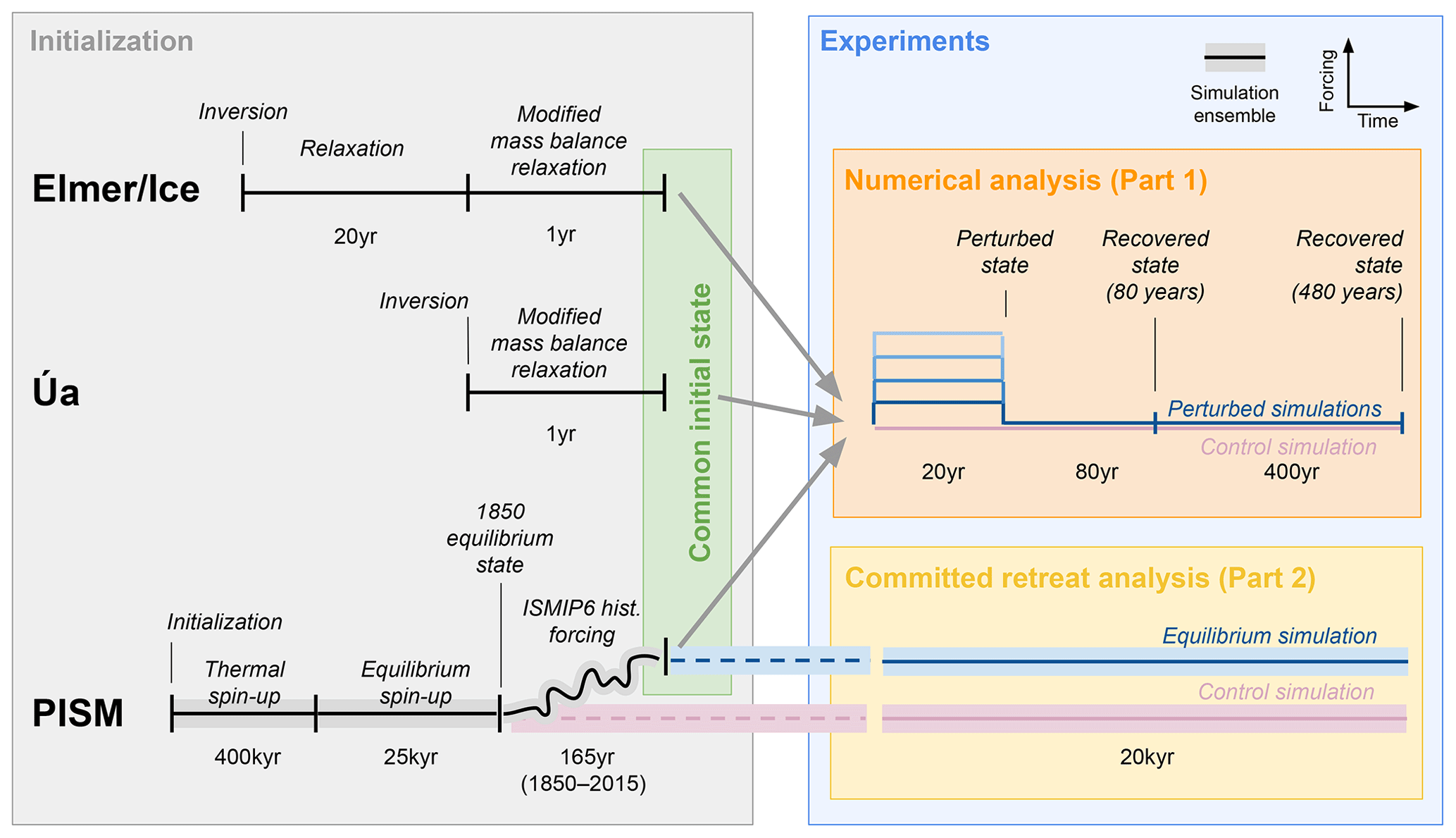
Figure 1 Overview of experimental set-up. Schematic summarizing the experimental set-up used in the stability analysis of the present-day Antarctic grounding lines. The set-up comprises the different model initialization procedures (grey box) as well as the two different types of prognostic model experiments (blue box): the numerical stability analysis presented in this article (Part 1; orange box) and the committed retreat analysis presented in Reese et al. (2023a) (Part 2; yellow box). The three different model initialization procedures yield three comparable initial states (“common initial state”; green box), from which all experiments are started. See text for more details.

2.1 Common approach

We first initialize all three models using as many common aspects of our models as possible to create initial states based on the observed geometry of the Antarctic Ice Sheet. These common inputs and approaches are summarized in Table 1. Namely, we use observations of bedrock topography, ice surface elevation, and ice thickness from BedMachine Antarctica (Version 2; Morlighem et al., 2020). To replicate the current ice flow, we take surface velocities from a recent snapshot in time (2015–2016) from the MEaSUREs Annual Ice Velocity Maps dataset (Version 1; Mouginot et al., 2019), which has a resolution of 1 km and good coverage across the entire ice sheet.

Across the surface of the ice sheet, all models initially apply a constant-in-time surface mass balance (later modified for Elmer/Ice and Úa), which is the output from the regional atmospheric climate model RACMO2.3p2 averaged from January 1995 to December 2014 (van Wessem et al., 2018). Melting at the bottom of ice shelves is a key control on the dynamics of the Antarctic Ice Sheet and is the focus of the perturbation experiments. All three models parameterize sub-shelf melt rates using their respective implementations of the Potsdam Ice shelf Cavity mOdel (PICO; Reese et al., 2018a). We ensure that the PICO geometry is the same as that in Reese et al. (2018a). PICO parameters were selected to reflect the sensitivity of sub-shelf melt rates in the Amundsen Sea Embayment (ASE) sector and Filchner–Ronne Ice Shelf to ocean temperature changes. Further details on this tuning of PICO parameters can be found in Reese et al. (2023a). This results in the parameter for vertical heat exchange ${\mathit{\gamma }}_T^{*}=\mathrm{5}\times {\mathrm{10}}^{-\mathrm{5}}$ m s⁻¹ and the parameter for the overturning strength C=2 Sv m³ kg⁻¹. While PICO is not a perfect representation of present-day melt rates, it can track the grounding-line movement and provides melting rates for newly ungrounded regions.

(Joughin et al., 2019)(Asay-Davis et al., 2016)(Schoof and Hindmarsh, 2010; Bueler and van Pelt, 2015)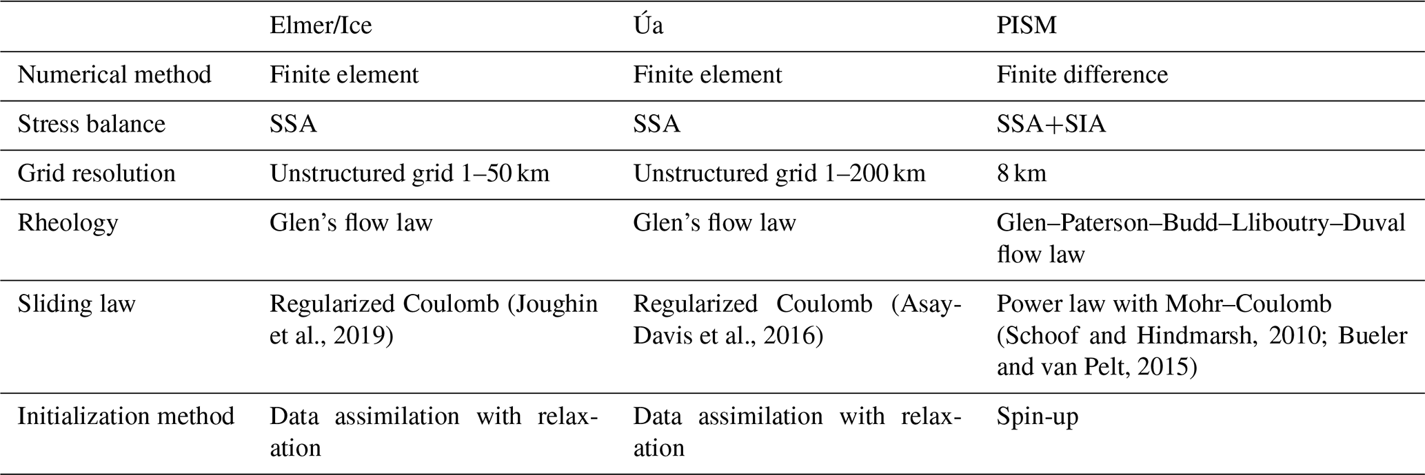

Table 1 Comparison of the models and the physics of the models which are detailed further in Sect. 2.1 and Appendix A1–A3. SSA: shallow-shelf approximation, SIA: shallow-ice approximation.

2.2 Steady states in Elmer/Ice and Úa

Elmer/Ice and Úa are both finite element models that solve the vertically integrated ice dynamics equations using the shallow shelf approximation (SSA; MacAyeal, 1989). Both models have been used extensively to solve ice flow problems in Antarctica and have participated in a number of model intercomparison experiments, e.g. Pattyn et al. (2012); Cornford et al. (2020). Both models first create an unstructured finite element mesh, where element sizes were refined in fast-flowing regions and close to the grounding line. The initial ice sheet model states were then obtained using a two-step approach outlined in the following sections.

2.2.1 Model inversions

Using present-day observations of ice sheet geometry and velocity, the models are first initialized using a model inversion to estimate sliding law and rheology parameters using the adjoint method (MacAyeal, 1993). Both models impose a pressure-dependent sliding law, which usually leads to more physically representative sliding close to the grounding line as compared to the Weertman sliding law (Brondex et al., 2019). The optimal fields for the basal slipperiness and viscosity parameters are found by minimizing a cost function, which is the sum of misfit and regularization terms. The main misfit term is the difference between observed and modelled velocities. Both models also apply an additional penalty on the rates of thickness change, to reduce nonphysical ice flux divergence anomalies. We regularize the inverse solutions using Tikhonov regularization terms that enforce smoothness of the inferred parameters (basal slipperiness and ice rate factor). The regularization weights are determined using an L-curve analysis. By design, at the end of the inversion the surface velocities are in very good agreement with observations. See Appendix A1 and A2 for details on the inversion.

2.2.2 Mass balance modification

Observations clearly show that the present-day geometry of the ice sheet is not in steady state; i.e. ice thickness changes through time $\mathrm{d}h/\mathrm{d}t\ne \mathrm{0}$, and the current mass balance is $\mathrm{d}h/\mathrm{d}t={\dot{m}}_{\mathrm{pd}}-\mathbf{\nabla }\cdot \left(\mathit{v}h\right)$ where v is the ice velocity and ${\dot{m}}_{\mathrm{pd}}$ is the total present-day mass balance (surface + base). However, given that stability is strictly speaking a property of steady states, in order to test the stability of the current grounding lines, we require a steady-state configuration of the ice sheet. Ideally, this steady state would be achieved through the inversion step. However, the penalty we apply to rates of thickness change is not sufficient to bring the model into a steady state, and when the model is run forward in time it drifts away from the present-day geometry and ice velocity. Hence, we create a modified mass balance term ${\dot{m}}_{\mathrm{mod}}$ such that $\mathrm{d}h/\mathrm{d}t=\mathrm{0}$ or as close as numerically possible. To do this, we follow a similar approach to others (Price et al., 2011; Goelzer et al., 2013) in which we subtract the modelled rates of ice thickness change ${\left.\mathrm{d}h/\mathrm{d}t\right|}_{\mathrm{relax}}$ needed to keep the model in balance from ${\dot{m}}_{\mathrm{pd}}$ as follows:

$$\begin{array}{}\text{(1)}& \begin{array}{rl}{\dot{m}}_{\mathrm{mod}}& ={\dot{m}}_{\mathrm{pd}}-{\left.{\displaystyle \frac{\mathrm{d}h}{\mathrm{d}t}}\right|}_{\mathrm{relax}},\\ & \text{where}{\dot{m}}_{\mathrm{pd}}={\dot{b}}_{\mathrm{RACMO}}+{\dot{b}}_{\mathrm{PICO}}.\end{array}\end{array}$$

Thereby, the present-day surface mass balance field ${\dot{b}}_{\mathrm{RACMO}}$ is the 1995–2014 averaged surface mass balance provided by RACMO2.3p2 (van Wessem et al., 2018) and ${\dot{b}}_{\mathrm{PICO}}$ the sub-shelf melt rates provided by PICO using 1975–2012 averaged ocean forcing from Schmidtko et al. (2014). By construction, the modification term ${\left.\mathrm{d}h/\mathrm{d}t\right|}_{\mathrm{relax}}$ reduces the mass balance to $\mathbf{\nabla }\cdot \left(\mathit{v}h\right)={\dot{m}}_{\mathrm{mod}}$ with $\mathrm{d}h/\mathrm{d}t\approx \mathrm{0}$. It is calculated in slightly different ways for the two models, the details of which are in Appendix A1 and A2. In summary, Elmer/Ice calculates ${\left.\mathrm{d}h/\mathrm{d}t\right|}_{\mathrm{relax}}$ after a 20-year relaxation period and then inputs this into a 1-year forward relaxation, which forms the beginning of the perturbation experiments. Úa uses a semi-iterative approach which takes ${\left.\mathrm{d}h/\mathrm{d}t\right|}_{\mathrm{inv}}$ calculated after the inversion as input to Eq. (1) for a 1-year relaxation period. The ${\dot{m}}_{\mathrm{mod}}$ field is then recalculated using ${\left.\mathrm{d}h/\mathrm{d}t\right|}_{\mathrm{relax}}$ at 1 year, and this is the beginning of the perturbation experiments. The modified mass balance fields and terms in Eq. (1) are shown in Figs. S1 to S3 in the Supplement.

We find that applying this modified mass balance term over the entire ice sheet (both grounded and floating portions) brings the ice sheet models to a steady state. However, by creating our modified mass balance field, we have created a surface mass balance field that deviates from climate conditions in RACMO. Broadly speaking, these fields represent the spatial pattern across the ice sheet; both models show higher positive mass balance around the coastal margins and more precipitation around the West Antarctic coast of the ASE and Bellingshausen Sea regions (Figs. S1 and S2). Additionally, the ${\left.\mathrm{d}h/\mathrm{d}t\right|}_{\mathrm{relax}}$ fields are regionally similar, where in both models the modification needed to obtain a steady state is largest in West Antarctica, in particular in the ASE sector. This reflects the current flux imbalance in West Antarctica and ongoing retreat and mass loss from this region. While the spatial patterns are broadly the same, e.g. large modifications across the ASE, we note that the distribution and amplitude of the modification to the mass balance vary greatly between the two models, likely due to subtle differences in our model initialization. In Úa the modification is higher in magnitude and locally spatially heterogeneous; i.e. both positive and negative values occur in close proximity to one another (see Fig. S3). By comparison, the modification in Elmer/Ice is smoother and generally smaller in magnitude. Crucially, it is assumed that modifying the mass balance in this manner has not altered the location of the critical thresholds in the grounding-line position for the real ice sheet and that perturbing these steady states can allow us to learn about the stability of the present-day grounding lines in their current position. Given the differences between our two modified mass balance fields, and our results are consistent for both models (and PISM does not modify the mass balance; Sect. 2.3), our results are unlikely to be an artefact of this field having a specific shape. We also conducted a series of numerical experiments where we allowed the grounding lines to drift instead of forcing them to be stationary. This was done by applying either limited or no additional modification to the surface mass balance (Fig. S3). In all cases we found that once the perturbation was removed, grounding lines started to drift at the same rate as the (unperturbed) reference run. For unstable states one would expect the trajectories to diverge with time.

2.2.3 Initial states

The initial ice sheet model states created by Elmer/Ice and Úa closely replicate the observed ice thickness and surface velocities, particularly in the location of fast-flowing ice streams (see Figs. S5 and S6). Importantly, the positions of the grounding lines in our models closely replicate the currently observed position of the grounding lines (Fig. 2) from BedMachine (Morlighem et al., 2020). In addition, the good agreement of observed and modelled grounding-line positions for all models can be seen in our individual glacier profile figures presented in the results (Fig. 4). We calculate the error in the grounded ice area (a proxy for grounding-line change), by differencing the simulated and observed grounded ice areas. To obtain a relative displacement of the grounding line itself, we normalize this area change by the simulated length of the grounding line. The resulting grounding-line position errors are 84 m for Elmer/Ice and 540 m for Úa. During a steady-state control simulation for both models, there is less than 4.2 mm of change in sea-level-equivalent volume over 100 years. Furthermore, there is very little drift in the position of the grounding line from the initial location, deviating by only 12.6 (Elmer/Ice) and 2.1 m (Úa) over 100 years, which is very small with respect to grid resolution (1 km close to the grounding line).

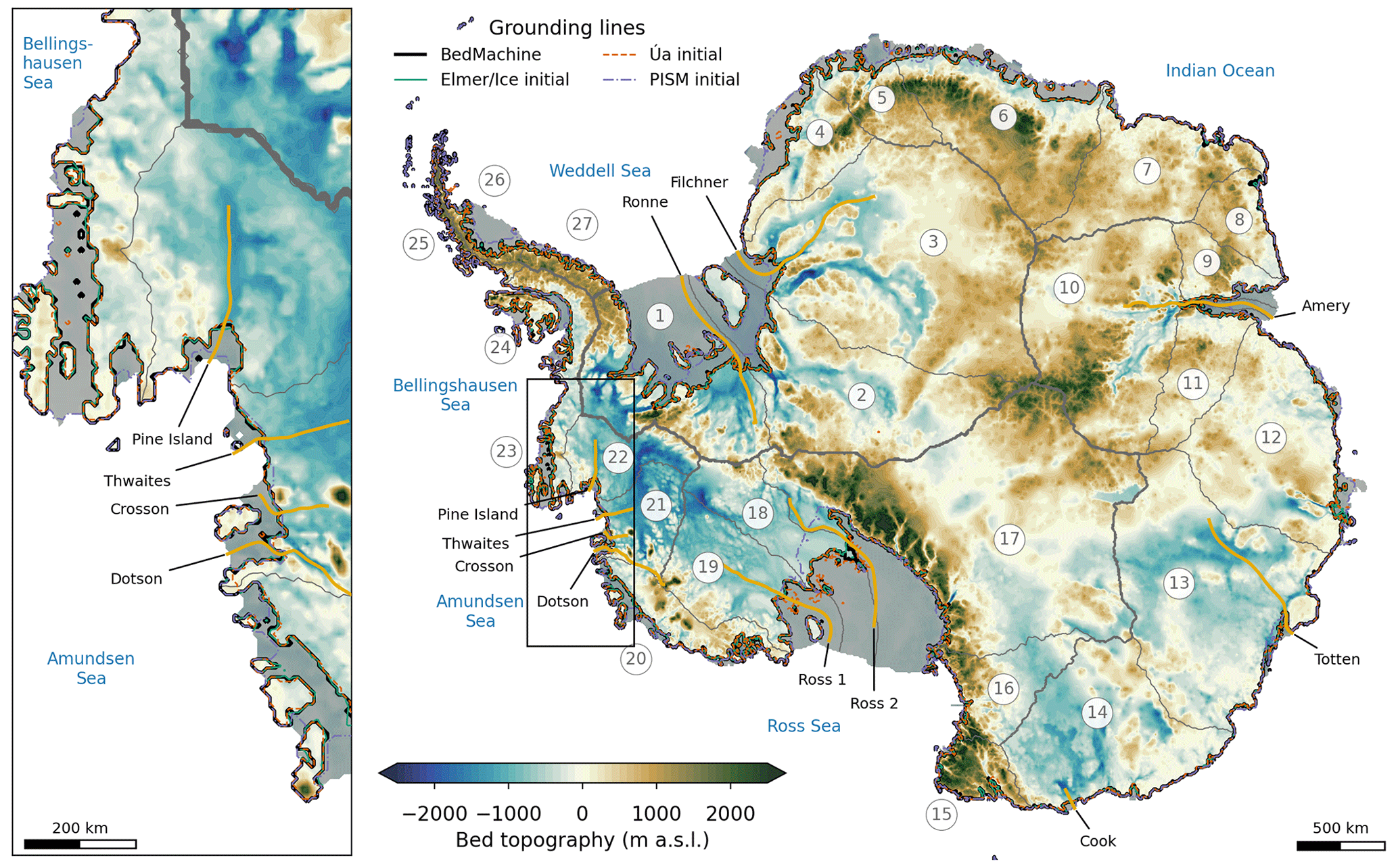
Figure 2 Modelled and observed present-day Antarctic grounding-line locations. Present-day Antarctic bed topography (BedMachine; Morlighem et al., 2020) showing regions where the bed topography is below (blue shading) and above (brown shading) sea level in metres above sea level (m a.s.l.). Modelled initial grounding-line positions are shown as coloured lines; observed grounding-line position is shown in black. Ice shelves are indicated by grey shading. Golden lines denote the locations of the transects shown in Fig. 4. Grey lines mark the boundaries of the IMBIE basins (Zwally et al., 2012). The inset shows a zoom into the Amundsen Sea Embayment sector of West Antarctica.

2.3 Transient state in PISM

To support the findings of this study further, we generate an initial state using PISM. Due to the spin-up procedure of PISM, when it arrives at a steady ice sheet state, by definition that state will be stable. Hence, we would not need to additionally perturb such a state to determine whether it is stable or unstable. Instead, we conduct the trajectory analysis described above whereby we perturb a state including a present-day trend in mass changes. This allows us to examine whether current grounding-line positions stay within the vicinity of the unperturbed control run. More details on the physics modelled in PISM and a comparison to the other models are given in Appendix A3.

2.3.1 Spin-up to pre-industrial conditions and historical run

The strategy adopted to build an initial state with PISM relies on spin-up methods, with the approach taken here detailed in Reese et al. (2023a) and summarized in Fig. 1: we first create a thermal equilibrium with fixed geometry, followed by an ensemble of equilibrium simulations with full dynamics run under constant ∼ 1850 climate conditions (here equilibrium is defined as the integrated ice sheet mass balance being close to zero).

Starting from the 1850 initial configurations, historic simulations are run from 1850 to 2015. We use ISMIP6 historic forcing for the atmosphere and the ocean from 1850 to 2015. Climatologies for the pre-industrial equilibrium state were created such that when adding the historic anomalies the atmosphere and ocean forcings between 1995 and 2014 match the present-day observations. Observed present-day velocities do not directly enter the initialization, but instead they are used, amongst other criteria, indirectly to determine optimal parameters in the initial state related to basal sliding and sub-shelf melting. We select the state that best replicates present-day ice thickness, grounding-line position, mass loss, and ice surface velocities for the “best” PICO parameters (“AIS5” in Reese et al., 2023a).

2.3.2 Initial state

Despite the different initialization procedure of PISM, the resultant ice sheet reference state with respect to geometry and ice velocities is in good agreement with observations and the states obtained in the other models. PISM is capable of locating most, if not all, ice streams in their correct positions and accurately replicating the observed ice thickness and surface velocities after the spin-up (see Figs. S5 and S6).

Due to the spin-up procedure and the coarser grid resolution of PISM, there are some areas with greater deviation in the initial grounding-line position. The overall error in the grounding-line position for PISM is 11.4 km, which, while higher than the other two models, is very close to the horizontal grid size used in the model. Overall there is good agreement between modelled and observed grounding-line positions (Fig. 2), including in regions of particular interest, such as Thwaites Glacier. The model grounding-line positions are calculated using the flotation criterion.

During the historic simulation (1850–2015), the change in sea-level-equivalent volume is −1.88 mm. While this is lower than observed rates of mass loss over the last decades, due to mass gains from snowfall, the pattern of thickness change is comparable to observations (see Reese et al., 2023a). During the control run the present-day climate conditions (2015) are held constant, so the climate forcing itself is steady, but the ice sheet state itself is not in a steady state (ice thickness changes through time are not equal to zero).

2.4 Experimental design

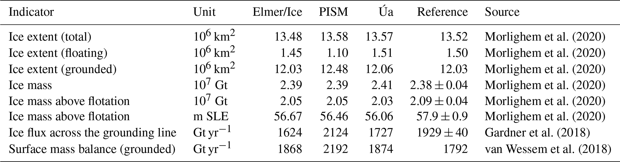
We have generated three ice sheet model initial states which closely replicate the current geometry, surface velocity, and grounding-line positions of the Antarctic Ice Sheet (Table 2). We account for any remaining discrepancies between individual models by running control simulations alongside the perturbation experiments, and the results presented are then with respect to these control runs.

Morlighem et al. (2020)Morlighem et al. (2020)Morlighem et al. (2020)Morlighem et al. (2020)Morlighem et al. (2020)Morlighem et al. (2020)Gardner et al. (2018)van Wessem et al. (2018)

Table 2 Comparison of the initial state indicators for the initial states created using Elmer/Ice, Úa, and PISM. All variables, except for flux across the grounding line, were calculated across the same 2 km resolution grid. Reference values for ice extents (total, floating, and grounded) were calculated using the BedMachine dataset (Morlighem et al., 2020), whereas ice mass values were taken from Table S3 in the dataset paper (Morlighem et al., 2020) (m SLE, metres sea level equivalent). The total flux across the grounding line was calculated in each respective model. Observed grounding-line flux was taken from Gardner et al. (2018), and total surface mass balance is from RACMO2.3p2 (van Wessem et al., 2018).

During the control simulations the mass balance in Elmer/Ice and Úa is

$$\begin{array}{}\text{(2)}& \mathbf{\nabla }\cdot \left(\mathit{v}h\right)+{\displaystyle \frac{\mathrm{d}h}{\mathrm{d}t}}={\dot{m}}_{\mathrm{mod}},\end{array}$$

where $\frac{\mathrm{d}h}{\mathrm{d}t}\approx \mathrm{0}$ and ${\dot{m}}_{\mathrm{mod}}$ are the same as defined for the previous models in Eq. (1). In PISM the mass balance is

$$\begin{array}{}\text{(3)}& \mathbf{\nabla }\cdot \left(\mathit{v}h\right)+{\displaystyle \frac{\mathrm{d}h}{\mathrm{d}t}}={\dot{m}}_{\mathrm{pd}}\end{array}$$

and $\mathrm{d}h/\mathrm{d}t\ne \mathrm{0}$, broadly comparable to present-day rates of ice thickness change.

We apply a perturbation to the current position of the grounding lines by increasing the far-field ocean temperature that drives the melt rates calculated by PICO. Note that, in general, it would be possible to perturb the system using a number of different control parameters in our models. Given the important role that ice shelves play on inland ice sheet dynamics and grounding-line position, via buttressing forces, we here choose to perturb the system by applying a shift in sub-shelf melt rates.

We increase the input ocean temperature, which is assumed to be representative of the conditions at depth on the continental shelf, by $\mathrm{\Delta }T\in \mathit{\{}\mathrm{1},\mathrm{3},\mathrm{5}\mathit{\}}$ ^∘C all around the Antarctic Ice Sheet. This perturbation in temperature is applied for 20 years to create a numerically significant grounding-line retreat. By applying different increases in ocean temperature, we are able to test the robustness of this perturbation and found that a 5 ^∘C perturbation over 20 years remained small; i.e. it resulted in a small but obvious deviation in the position of the grounding line. While +5 ^∘C appears to be an unrealistically high magnitude change, we want to stress that this perturbation is not designed to be realistic and is only applied over a few decades. Instead, we can think of our small perturbation as a small movement of the grounding line away from its current position, on the order of a few grid cells or ice thicknesses at the grounding line. Indeed, the +5 ^∘C perturbation leads to approximately 10 km of retreat along the profiles in the ASE region (see Results) and along other profiles (see Figs. S16 and S17). We note that a recovery for the +5 ^∘C perturbation also implies that a smaller perturbation would also be reversible and indicates that the steady state is stable.

Across the floating ice shelves, during the 20-year perturbation, the mass balance ${\dot{m}}_{\mathrm{\Delta }T}$ is the anomaly in sub-shelf melting calculated using PICO $\mathit{\delta }{\dot{b}}_{\mathrm{PICO}}$ applied to the modified mass balance fields in Elmer/Ice and Úa as

$$\begin{array}{}\text{(4)}& \begin{array}{rl}{\dot{m}}_{\mathrm{\Delta }T}& ={\dot{m}}_{\mathrm{mod}}+\mathit{\delta }{\dot{b}}_{\mathrm{PICO}}\text{where}\mathit{\delta }{\dot{b}}_{\mathrm{PICO}}\\ & ={\dot{b}}_{\mathrm{PICO}}(T+\mathrm{\Delta }T)-{\dot{b}}_{\mathrm{PICO}}\left(T\right).\end{array}\end{array}$$

Across the grounded areas no perturbation is applied, and the mass balance is unchanged (Eq. 1).

In PISM the mass balance field has not been modified from present-day conditions, and unlike the other two models the initial temperatures T in PICO are perturbed directly by ΔT

$$\begin{array}{}\text{(5)}& {\dot{m}}_{\mathrm{\Delta }T}={\dot{b}}_{\mathrm{RACMO}}+{\dot{b}}_{\mathrm{PICO}}(T+\mathrm{\Delta }T).\end{array}$$

We compare the integrated sub-shelf melt perturbation applied in all three models and find that it is comparable for all experiments (see Fig. S10b).

After 20 years we remove the perturbation and allow a recovery phase of the simulation for a further 80 years (Fig. 1). We extend some simulations by 400 years to test the robustness of the grounding-line evolution over longer timescales. Throughout the forward-in-time experiments, the extent of the ice shelves remains unchanged; however, all models impose a minimum ice shelf thickness, which is sufficiently thin to represent ice that has been removed and provides no buttressing.

During the recovery phase (80–480 years after the end of the perturbation), we examine the temporal evolution of the integrated ice flux across the grounding line. We choose grounding-line flux as our metric of the system state because it is found to recover faster to a perturbation than grounded area or volume, due to the long timescales needed for the ice to thicken and re-advance. In the steady-state initial states of Úa and Elmer/Ice, by design, the ice flux across the grounding line balances the surface accumulation upstream. Increased sub-shelf melt in our simulations leads to a sharp increase in ice flux across the grounding line, which is assumed to be due to a loss of buttressing as a result of ice shelf thinning. If the flux across the grounding line returns to its initial value after the perturbation is removed, this indicates that the ice sheet reverts to a steady state with a balance between surface accumulation in the grounded regions and grounding-line flux (note that surface accumulation is altered a little by the grounding-line movement). Hence, it is assumed that a return of the grounding-line flux indicates the grounding line has either reverted back to its initial position or has begun to re-advance towards its former position. When the grounding line does not retreat further, it means that it has found a new stable position very close of the previous one. If the flux were to increase away from its initial value, the grounding line is unstable. To support this we also examine the trend in grounded-line position after the perturbation is removed, which is calculated as the change in grounded area for a constant grounding-line length.

To further analyse the response of the grounding lines after the perturbation is removed, we calculate the e-folding relaxation time, i.e. the time taken for the flux to decrease by a factor of e (Euler's number; ≈2.17). To do this we fit an exponential decay function in the form

$$\begin{array}{}\text{(6)}& \mathrm{\Delta }Q\left(t\right)=\mathrm{\Delta }{Q}_{\text{pert}}{e}^{-t/\mathit{\tau }}\end{array}$$

to the change in flux during the recovery period of 80 years ΔQ(t), where ΔQ_pert is the change in flux at the end of the 20-year perturbation relative to the initial, unperturbed flux. t is time after the perturbation, and τ is the recovery timescale. We repeat this for all three models and perturbation experiments, and these exponential curves can be seen in Figs. S7 to S9.

3 Results

In the following sections we present the results of our perturbation experiments of present-day Antarctic grounding lines as described in Sect. 2.4. Figure 3 shows the integrated ice flux across the entire Antarctic grounding lines in each model during the perturbation experiments. We also present the results integrated across the 27 basins used in the Ice Sheet Mass Balance Inter-comparison Exercise (IMBIE) (Fig. 2; Zwally et al., 2012), excluding basins 7, 8, and 25, which contain only small ice shelves. Additional figures showing grounding-line position change and volume above flotation can be found in the Supplement (Figs. S10 to S15).

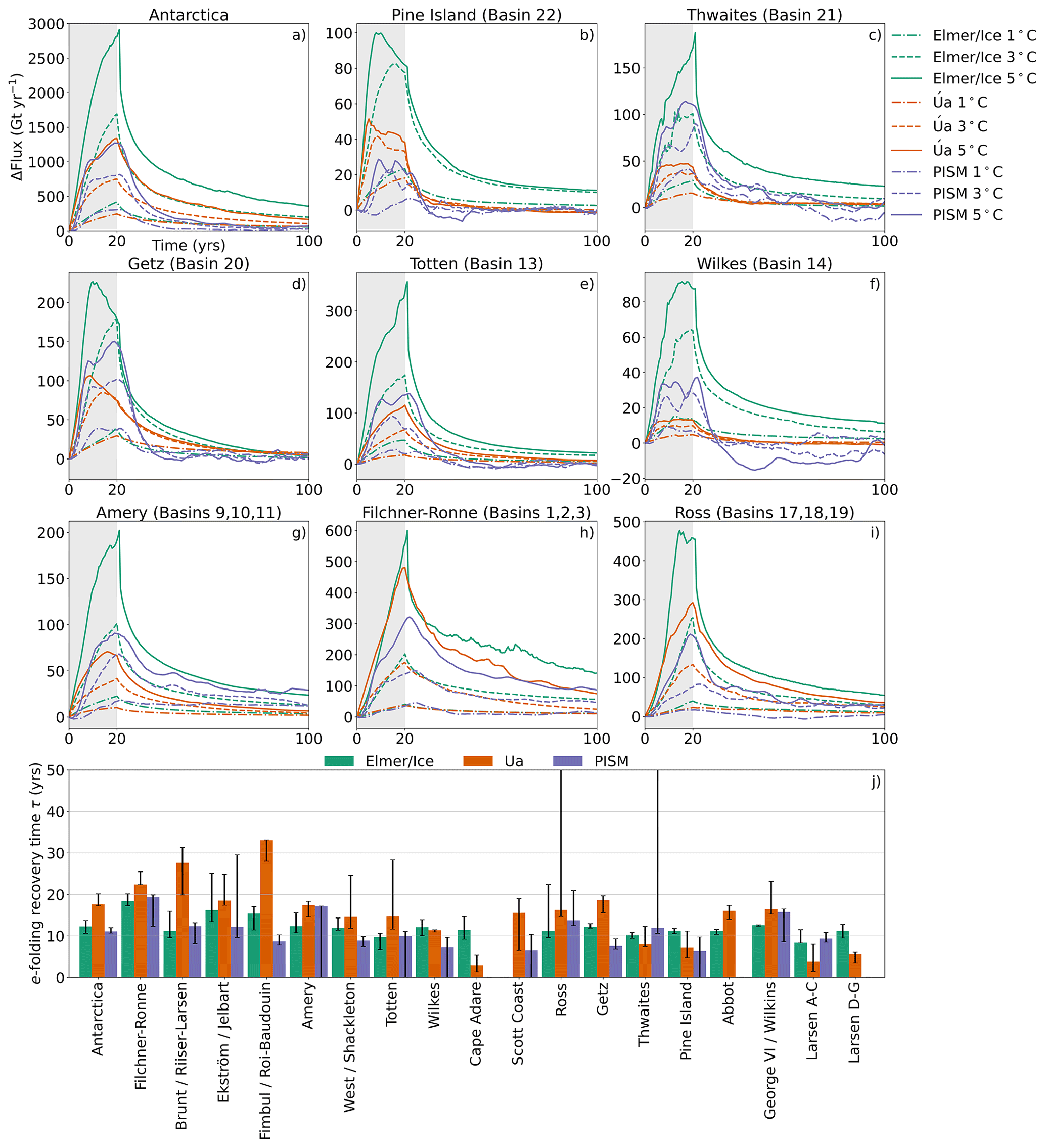
Figure 3 Reversibility experiments and recovery timescales. Change in integrated ice flux across the grounding line for perturbed simulations using three ice sheet models. All three temperature perturbation experiments (1, 3, 5 ^∘C) are shown for selected individual basins. For ease we merge the results for basins flowing into the Amery, Filchner–Ronne, and Ross ice shelves. See Fig. S11 for additional basins. PISM fluxes are smoothed using a running mean filter of 5 years. Grey shading shows the perturbation period. Bar plot shows the e-folding recovery time. Each bar shows the median response time from all three experiments (1, 3, 5 ^∘C) for each model, and error bars show the range. Bars are not shown for individual models for some basins (e.g. Cape Adare for PISM) where the exponential fit to the change in ice flux was deemed poor and the R² value is less than 0.8. There are four individual experiments for PISM where the flux results are noisy (due to coarser grid resolution) such that the exponential fit for that individual temperature perturbation has R²<0.8 (see Fig. S8). We set these values to zero as the lower end of the error bars.

3.1 Antarctic Ice Sheet

On the Antarctic-wide scale, all models and all perturbations show a similar trend: a strong increase in ice flux, reaching a maximum at the end of the 20-year perturbation period, followed by an exponential decrease for the remaining 80 years (Fig. 3). The magnitude of the flux response to the melt perturbations is comparable between all ice sheet models, in particular for the 1 ^∘C temperature experiment, in which ice flux increased by approximately 300 Gt yr⁻¹. In the higher temperature scenarios (3 and 5 ^∘C), the flux responses diverge slightly from one another; PISM and Úa remain similar, while Elmer/Ice shows a stronger increase. This is likely due to subtle differences in the imposed basal melt perturbation in each model, which also diverge with the magnitude of the perturbation (see Fig. S10b).

The calculated e-folding flux response time reveals that the Antarctic-wide recovery time is in good agreement for all models, ranging between 10 and 20 years, and is largely independent of the magnitude of the perturbation (Fig. 3, bottom panel). During the 80-year recovery period, the flux decreases rapidly but is not fully recovered. To check whether it is able to recover eventually, we extended the relaxation period in the 5 ^∘C simulations in all models to 480 years and found that the Antarctic-wide flux returns to within 3.5 % of its original value (see Fig. S13). Alongside the ice flux evolution, the total retreat of the grounding line and ice volume show similar trends: rapid retreat and reduction in ice volume during the perturbation, after which retreat rates subside and grounding lines begin a slow recovery. Furthermore, for the Antarctic-wide signal there is no indication of accelerated retreat (see Fig. S10). The recovery of the ice flux, alongside a short, 2-decade e-folding time, strongly indicates that the majority of Antarctic grounding lines are reversible. Also, ice flux evolution for individual basins (in all models) appears to show an exponential decrease after the perturbation is removed (Fig. 3). However, some basins recover more quickly than others. In the remainder of this section we explore the response of individual basins in more detail.

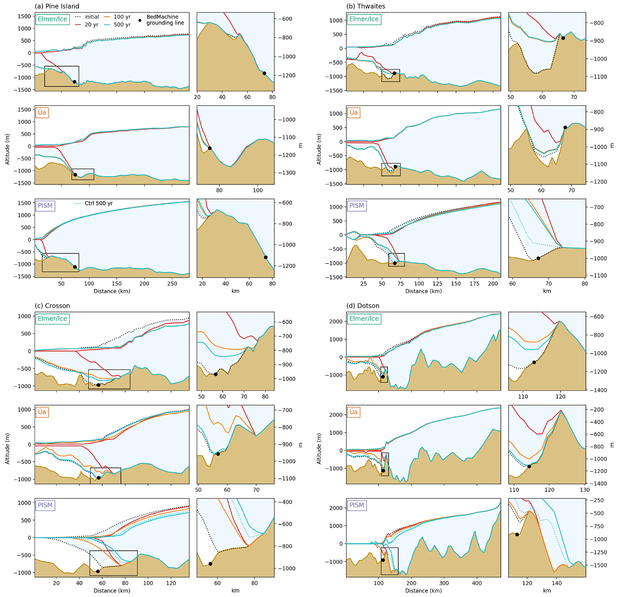
Figure 4 Profiles of the Amundsen Sea Embayment (ASE) sector for the three models at different time intervals during the 5 ^∘C experiment. Shown are the ice sheet geometries of the initial state (dotted line filled with light blue), at the end of the perturbation at 20 years (red line), after 80 years of recovery at 100 years (orange line), and after 500 years (cyan line). The dotted cyan line shows the location of the control simulations after 500 years for the PISM simulations. Observed (BedMachine) grounding-line positions are indicated by a black dots. The small panels show a zoom into the region marked by the black squares. The resolution of each profile depends on the model resolution. Profile locations are shown in Fig. 2.

3.2 Amundsen Sea Embayment sector

The Amundsen Sea Embayment (ASE) sector encompasses the Pine Island, Thwaites, and Getz drainage basins (basin numbers 20 to 22 in Fig. 2). For all three of these basins, our results show a rapid exponential decay in the ice flux (e-folding times <20 years) after the 20-year perturbation (Fig. 3). We extract profiles along four marine glaciers in the ASE sector (Fig. 4) to show the response of a vertical transect along the ice shelves at four critical points of the 5 ^∘C experiment. These flow lines were directly interpolated from the original model grids. We note some differences in the bed geometry due to the different resolution and interpolation methods used by each model.

At Pine Island Glacier, the initial grounding-line position in Úa is close to observations, whereas in Elmer/Ice and PISM the initial grounding-line positions are located downstream at a topographic ridge (Fig. 4a). Grounding lines in Elmer/Ice and Úa retreat approximately 3 to 7 km (Fig. S12) across sections of retrograde sloping bed topography during the perturbation. In PISM the grounding line retreats along a section of pro-grade slope to the top of the ridge. For all models the 5 ^∘C perturbation causes the ice shelf to disappear entirely. After the perturbation is removed, grounding lines in all models advance back to their initial positions and the ice shelves regrow to their initial thickness. Grounding-line flux (Fig. 3) increases during the 20-year perturbation and sharply decreases thereafter. At year 50 the flux in Úa and PISM has decreased either below the control simulation (PISM) or within 0.7 % (Úa) of the initial flux. In Elmer/Ice the recovery is slower (11-year e-folding time) than the other models, and the flux remains 10 % higher than the initial flux at year 100.

Our results for Thwaites Glacier are similar to Pine Island (Fig. 4b). In the entire Thwaites basin (including Dotson and Crosson ice shelves) grounding-line flux increases between 50 and 170 Gt yr⁻¹ during the perturbation, and then it decreases rapidly (response times 8–15 years) in all models after the perturbation is removed. At Thwaites Glacier, the initial grounding lines in all three models are in close agreement with one another (Fig. 4b). For Elmer/Ice and Úa this is slightly downstream of the observed grounding-line position at a topographic ridge, whereas PISM is located at the currently observed position. The retreat during the perturbation is not across a section of reverse bed slope, but instead it remains downstream of a second topographic ridge (located 70 km along the profile). For PISM and Úa, the ice shelf thins strongly during the perturbation, whereas in Elmer/Ice, the ice shelf is relatively thick in the initial state and does not disappear during perturbation. After the end of the perturbation, the ice shelf grows back to its initial shape in all models. In Úa the grounding lines re-advance fully to their initial positions (within 100 years), and PISM re-advances to the position arrived at in the control simulation after 500 years. The recovery in Elmer/Ice is slower than Úa, which corresponds to the longer recovery timescale for the entire Thwaites basin (Fig. 3).

Similar behaviour is also observed for Crosson and Dotson ice shelves for Elmer/Ice and Úa (Fig. 4c–d). The ice shelf thins and the grounding line retreats across a prograde slope during the perturbation. The grounding lines advance towards their initial position after the perturbation is removed, and in Úa it returns fully to its former position after 500 years. In contrast, the Crosson and Dotson grounding lines in PISM show signs of ongoing retreat. Crucially, the grounding lines in PISM start in slightly retreated positions compared to those of observations and the two other models. After the perturbation (20–100 years) the ice shelves thicken and the grounding lines re-advance. However, after 100 years, the ice surface lowers and the grounding lines retreat to a location further inland of the perturbed position (at 20 years). Importantly, the grounding-line positions at year 500 are very similar to their location in the control simulation, showing that they are reversible with respect to the trend in the control simulations. Long-term (10 000-year) simulations under present-day climate forcing also show that the Crosson and Dotson grounding lines will remain (in the absence of additional forcing) at this slightly retreated position in the future (see Fig. 4 in Reese et al., 2023a).

For additional basins in this region of West Antarctica, the Getz (Fig. 3) and those in the Bellingshausen Sea sector (basins 23 and 24 in Fig. S11), the results are similar: the ice flux tends toward its initial value, the grounding lines re-advance to their former positions (Fig. S12), and the response times are less than 20 years (Fig. 3). In summary, despite strong ice shelf thinning and retreat of the grounding lines in the ASE sector of the ice sheet during our perturbation experiments, we find that the grounding lines return to their initial positions after the perturbation is removed.

3.3 East Antarctica

Our experiments for basins in East Antarctica show a similarly strong signal of recovery to those in the ASE region. In particular, Wilkes, Totten, and Amery basins all display a rapid exponential decay in flux (e-folding times <20 years) after the perturbation is removed (Fig. 3). The flux in these basins appears to be reversible in Úa and PISM within 100 years and within 500 years in Elmer/Ice (Fig. S15). Grounding lines in these basins also show a strong signal of re-advance after the perturbation is removed (Fig. S12). This is also evident in selected glacier profiles at Totten and Cook glaciers (Fig. S17b–c). At both glaciers, the ice shelves disappear under the strongest perturbation (5 ^∘C), but at year 100 the ice shelves have almost recovered their former ice thickness and grounding-line positions. At Cook Glacier the grounding lines have fully returned to their initial positions after 500 years in Úa and PISM, and in Elmer/Ice it tends towards the initial position. At Totten Glacier, all models start close to the observed grounding-line position and retreat approx. 3 to 6 km inland (Fig. S12). After the perturbation is removed, Úa fully recovers by 500 years and Elmer/Ice has regrounded at the observed position (Fig. S17). In PISM the grounding line has not reverted to its initial position after 500 years but has instead approached the same location in the control simulation and can therefore still be considered reversible.

At Amery Ice Shelf, all models show that the ice shelves thicken, and the ice flux has almost fully recovered within 100 years, but the grounding line has not returned to its former position. However, it appears to have found a new stable grounding-line position within a short (approx. <10 km) distance inland, and it does not experience accelerated retreat thereafter (Fig. S17a). We note that a number of smaller basins surrounding Totten, Wilkes, and Amery (basins 12, 15, and 16) show a similar recovery of the ice flux within approximately <20 years and re-advance of the grounding lines.

In Dronning Maud Land (basins 4, 5, and 6), the signal of recovery is similar; all three ice sheet models show an increase in ice flux and retreat of the grounding line during the perturbation and a decreasing trend in ice flux after the perturbation is removed (Figs. S11 and S12). In general, the recovery of the grounding-line position is slower in these basins (e-folding times >15 years; Fig. 3). However, the extended relaxation period shows that the flux in the 5 ^∘C experiment recovers to within 3 % of its initial value for all models and all three basins (4–6). Concurrently, all grounding lines slowly re-advance to their former positions and show no signs of accelerated retreat.

3.4 Filchner–Ronne and Ross ice shelf sectors

Elsewhere, the large basins draining into the Filchner–Ronne and Ross ice shelves show more complicated behaviour. In general, we do not see any strong signs of instability; i.e. the flux decays towards its initial value after the perturbation is removed, similar to the previously discussed basins. However, for the Filchner–Ronne basin in particular, the ice flux in all models remains 20 %–40 % away from its initial value after the 80-year relaxation period in the 5 ^∘C experiment, and all models show response times of approximately 20 years (Fig. 3). In addition, all models show some signs of further retreat after the perturbation is removed (between 20–100 years in Fig. S12) but at a reduced rate. However, we find that in our extended simulations (for 5 ^∘C) the grounding lines either (1) tend to re-advance towards their initial positions, (2) show a re-advance of a few to several kilometres before appearing to reach a new steady position (Fig. S14), or (3) settle on a slightly retreated position a short distance inland. In no case do we see further retreat inland by the end of the simulations after 500 years. For both the Filchner–Ronne and Ross basins, the flux decreases to within 10 % (Elmer/Ice) or 6 % (PISM and Úa) of its initial value after 500 years.

We extract profiles at major outlets feeding into the large Filchner–Ronne and Ross ice shelves (see Fig. S16). For both profiles feeding the Ross Ice Shelf and the Ronne Ice Shelf, all models show signs of thinning and some additional retreat after the perturbation is removed (between 20 and 100 years). However, during the extended relaxation period (100 to 500 years), the ice shelves have begun to thicken again and the grounding lines do not retreat further inland. In the Filchner profile we find similar behaviour, with some additional retreat after the end of the perturbation (20 years). The grounding lines in PISM and Elmer/Ice do not retreat further after 100 years but remain in the same (slightly inland) position. In Úa the grounding line begins to re-advance and has almost returned to its initial (and full) ice shelf extent after 500 years. Overall, there are no signs of accelerated retreat in these basins, and instead the grounding lines of the larger ice shelves may need longer to recover from a perturbation.

4 Discussion

The perturbation experiments described above all showed that with time the grounding lines reverted back towards the state prior to the application of the perturbation. Where we ensured that the initial state was steady, as done in experiments using Elmer/Ice and Úa, the grounding lines migrated back to their original steady-state locations. Hence, these steady states are stable. In other experiments, where the grounding lines were allowed to migrate freely following the initialization procedure, the grounding-line migration rates reverted back to those of the reference (i.e. unperturbed) runs. In no experiments conducted with the three ice-sheet models did we see any indication of self-enhanced irreversible retreat from the currently observed locations of the grounding lines of the Antarctic Ice Sheet.

Previous studies have suggested that the retrograde bed slopes of Pine Island and Thwaites glaciers may mean they could undergo phases of internally driven (MISI) retreat (e.g. Joughin et al., 2010; Rignot et al., 2014; Joughin et al., 2014; Favier et al., 2014; Mouginot et al., 2014; Seroussi et al., 2017; Milillo et al., 2022). Our results suggest that the current grounding lines in the ASE sector of West Antarctica are reversible in response to a small deviation from their current position. While previous work has indeed shown that the bed topography further inland could cause tipping points to be crossed at Pine Island Glacier (Rosier et al., 2021), our results show that it is unlikely that the current retreat of Pine Island is due to MISI. Importantly, once the grounding line retreats further towards the critical regions identified in Rosier et al. (2021), internal instability is likely to be found.

We find similar results for Thwaites Glacier where an entire removal of the ice shelf (in the strongest perturbation) is not sufficient to destabilize the current grounding-line position, as has been suggested by previous studies (e.g. Wild et al., 2022). Several modelling studies have also shown that once the grounding lines retreat further inland under future increases in ocean forcing (and in the absence of any changes in surface mass balance from present day), it is possible that they will enter phases of accelerated retreat (Joughin et al., 2014; Seroussi et al., 2017). This accelerated retreat could be an indication of the onset of MISI. Note however that the projected grounding-line evolution of Thwaites Glacier in response to future ocean changes is associated with large uncertainties (Nias et al., 2019; Robel et al., 2019). To assess whether present-day Antarctic grounding lines are committed to enter irreversible retreat under current climate forcing, we conduct multi-millennial-scale simulations using an ensemble of present-day configurations in PISM (including the state used here); see our accompanying paper (Reese et al., 2023a). Indeed, we find that current climate conditions can force grounding lines in the ASE sector to eventually enter irreversible retreat but not within 300 years of constant present-day climate. This supports previous suggestions that present-day climate conditions may be sufficient to trigger rapid grounding-line retreat in West Antarctica in the long term (Golledge et al., 2021; Garbe et al., 2020; Joughin et al., 2014).

While our experiments, performed with three different ice sheet models, have shown consistent results, in the following paragraphs we note several caveats and potential sources of uncertainty. First, we parameterize the sub-shelf melt rates using the PICO sub-shelf melt model. While any parameterization of sub-shelf melt has associated uncertainties and may not capture certain physical processes in sub-shelf cavities, the sub-shelf melt distribution is not considered to greatly influence our results for two main reasons. First, our results are consistent across a wide range of temperature perturbations, including the strongest perturbation (+5 ^∘C) in which several ice shelves disappear. Second, our results are consistent across all three models despite the different implementations of PICO, which lead to subtly different melt rate distributions. In addition, we could have perturbed the grounding line using different model parameters, e.g. relating to ice viscosity or basal sliding. Indeed, we modified the basal sliding using Úa, and the results were consistent with those presented here; grounding lines re-advanced after the perturbation was removed.

Secondly, the results of our experiments are dependent on accurate representations of the ice thickness and bedrock topography. One approach to assess the impact of ice thickness and bedrock topography on our results would be to conduct additional perturbation experiments with modifications to the topography within some bounds. In part, we have achieved this by using three different ice sheet models with different grid resolutions, where in particular the bed topography around the grounding lines in PISM is smoother than the other models (see Fig. 4). Grid resolution itself is a source of uncertainty in ice sheet model simulations, in particular around the grounding line (Durand et al., 2009; Pattyn et al., 2013), but again this is captured by our experiments with different models and grids. In addition, we repeated some experiments in Úa in which we modified the mesh resolution around the grounding line and found that our results were not affected by a finer resolution (500 m) at the grounding line.

An additional source of uncertainty in our results is the absence of dynamic calving front positions in our models. In Elmer/Ice and Úa the ice front is fixed and the ice shelves maintain a numerically required minimum thickness, due to the numerical challenges of removing ice entirely from the domain. It is possible that this thin layer of ice promotes ice shelf regrowth at a quicker rate than a true re-advance of the ice front, due to the external forcing, surface, and basal mass balance, which are still applied across areas that have reached the minimum ice thickness. However, we note that the experiments conducted with PISM show similar recovery timescales, where in this case ice shelf cells are converted to ocean cells when the ice thickness decreases to zero. In addition, as the calving fronts are kept fixed, they are unable to advance beyond our prescribed initial position, which could also alter the stability of the grounding lines. We do not expect this to be relevant, because previous studies have shown that downstream regions (close to the calving fronts) of ice shelves provide little to no buttressing to upstream flow (Fürst et al., 2016; Reese et al., 2018b). We acknowledge that an evolving calving front may produce different results, especially as recent work has shown that (in the presence of buttressing) iceberg calving could impact the stability regime of grounding lines (Haseloff and Sergienko, 2022). Future studies should seek to include calving in such stability analyses.

Alongside calving, ice shelf damage can have an important impact on the magnitude of grounding-line retreat due to weakening in the shear zones (Lhermitte et al., 2020). Hence, it is possible that, with damage included, the retreat of the grounding line in our perturbation experiments would be larger. However, damage is not yet sufficiently well parameterized for inclusion in our models, and implementing time-dependent damage in particular is an ongoing (computational) challenge. An additional source of uncertainty is that we do not incorporate the surface melt elevation feedback during our simulations (Sergienko, 2022). Another point to make is that in our study here we only consider steady climate conditions in our experiments. Studies have shown that variability in the climate can cause noise-induced tipping, which causes a system to transgress towards a qualitatively different state before the actual tipping point is crossed (e.g. Ashwin et al., 2012). Future work would benefit from incorporating time-varying climate conditions to explore the possibility of noise-induced tipping in the real Antarctic Ice Sheet.

5 Conclusions

Our key finding is that the grounding lines of Antarctica, including Pine Island and Thwaites glaciers, show no indication of marine ice sheet instability (MISI) in their current state. We arrive at this conclusion by showing the existence of stable steady-state model configurations of the Antarctic Ice Sheet which closely resemble the observed present-day configuration as well as by showing reversibility of transient model configurations of the Antarctic Ice Sheet, under steady climate conditions. Our results indicate that MISI is not causing the present-day grounding-line migration.

There is a general consensus within the ice sheet modelling community that the West Antarctic Ice Sheet is susceptible to MISI. Here, we have argued that the currently observed changes of the Antarctic Ice Sheet are not a manifestation of ongoing positive feedback related to MISI. While our experiments suggest that an internal instability threshold has not yet been crossed in Antarctica, future retreat driven by changes in climate conditions could force the grounding lines to cross a tipping point, after which retreat becomes driven by MISI. Further work is needed to quantify the amplitude and duration of forcing required for the Antarctic Ice Sheet to enter a phase of a large-scale irreversible collapse involving grounding-line retreat over hundreds of kilometres and a concomitant sea level rise of potentially several metres.

Appendix A: Ice sheet models

A1 Elmer/Ice

A1.1 Model description

Elmer/Ice (https://elmerice.elmerfem.org/, last access: 25 July 2023) is an open-source finite element software for ice sheets, glaciers, and ice flow modelling built on the multi-physics finite element model suite Elmer (Ruokolainen et al., 2023). Elmer/Ice is a very general and flexible tool and as such has been used for a large diversity of applications (181 publications since 2004). The main features and capabilities of Elmer/Ice have been described in Gagliardini et al. (2013) and in the associated publications (https://elmerice.elmerfem.org/publications, last access: 25 July 2023). Here, only the main characteristics relevant for our analysis will be presented. Regarding the physics included in Elmer/Ice, the ice flow velocity is computed solving the shallow shelf approximation (SSA) assuming an isotropic rheology following Glen's flow law. The initial viscosity field is computed using the 3D ice temperature field given by Van Liefferinge and Pattyn (2013) and using the values given in Cuffey and Paterson (2010) for the activation energies and prefactors used to compute the temperature-dependent rate factor A in Glen's flow law. This initial viscosity is then modified using inverse methods. Regarding the boundary conditions, the ice front of ice shelves is assumed to be fixed (i.e. the sum of calving flux and frontal melt flux equals the ice flux at the front). For the grounded part, the sliding-law parameter field is inferred using inverse methods (see Sect. 2.2). For the floating part of the basal boundary, basal melt from the ocean is applied using the PICO model (Reese et al., 2018a), and no melt is applied to partially floating mesh elements. The grounding line is determined using a flotation criterion, and a sub-grid scheme is applied for the basal drag over partially floating elements: SEP3 in Seroussi et al. (2014). Regarding the mesh, we use an anisotropic mesh adaptation scheme that uses the observed ice velocities and thickness. The mesh is preferentially refined along the directions of highest curvature of these two fields with an additional criterion function of the distance to the grounding line. The resulting mesh contains 545 837 nodes and 1 070 444 linear elements, and the size varies from 1 km close to the grounding line to 50 km in the interior. The mesh is held constant during the transient simulations.

Details concerning the model initialization, relaxation, and the basal sliding law used in the transient simulations are given below.

A1.2 Model inversion

To initialize the model, we use an inverse method to estimate model parameters that control the basal slipperiness and the ice rate factor by minimizing the misfit between observed (u_obs) and modelled (u_mod) velocities. We optimize β in a linear sliding law that relates the basal shear stress, t_b, to the basal sliding velocity, v_b:

$$\begin{array}{}\text{(A1)}& {\mathit{t}}_{\mathrm{b}}=-{\mathrm{10}}^{\mathit{\beta }}{\mathit{v}}_{\mathrm{b}}=-C_{\mathrm{eff}}{\mathit{v}}_{\mathrm{b}}.\end{array}$$

This ensures that C_eff=10^β is positive. For the ice rheology, the vertically averaged effective viscosity used in the SSA is written as

$$\begin{array}{}\text{(A2)}& \begin{array}{rl}\overline{\mathit{\mu }}& ={\mathit{\eta }}^{\mathrm{2}}{\overline{\mathit{\mu }}}_{\mathrm{ini}}{I}_D^{(\mathrm{1}-n)/n},\\ & \text{with}{\overline{\mathit{\mu }}}_{\mathrm{ini}}=\mathrm{1}/H\underset{z_{\mathrm{b}}}{\overset{z_s}{\int }}(\mathrm{2}A{)}^{-\mathrm{1}/n}\mathrm{d}z,\end{array}\end{array}$$

where n is the Glen exponent, I_D is the second invariant of the strain-rate tensor D defined as $I_D^{\mathrm{2}}=\mathrm{2}\mathit{D}:\mathit{D}$, and ${\overline{\mathit{\mu }}}_{\mathrm{ini}}$ is the initial vertically averaged ice rigidity computed using the 3D ice temperature field given by Van Liefferinge and Pattyn (2013) as explained above; to ensure that the viscosity remains positive, we optimize the parameter η starting from an initial guess of one (i.e. no modification from the viscosity initially predicted from the temperature field).

We apply a standard inverse methodology in which a cost function J(β,η), which is the sum of misfit (I) and regularization (R) terms, is minimized. The gradients of J with respect to β and η are determined in a computationally efficient way using the adjoint method. The misfit I and regularization R terms are defined as

$$\begin{array}{}\text{(A3)}& {\displaystyle }I={\displaystyle \frac{\mathrm{1}}{\mathrm{2}}}\sum _{i=\mathrm{1}}^{N_{\mathrm{obs}}}\Vert {\mathit{u}}_{\mathrm{mod}}^i-{\mathit{u}}_{\mathrm{obs}}^i{\Vert }^{\mathrm{2}}\text{(A4)}& {\displaystyle }\begin{array}{rl}R& ={\mathit{\lambda }}_{\mathrm{1}}{\displaystyle \frac{\mathrm{1}}{\mathrm{2}}}\underset{\mathrm{\Omega }}{\int }(\mathbf{\nabla }\cdot ({\mathit{u}}_{\mathrm{mod}}h)-\dot{a}{)}^{\mathrm{2}}\mathrm{d}\mathrm{\Omega }\\ & +{\mathit{\lambda }}_{\mathrm{2}}{\displaystyle \frac{\mathrm{1}}{\mathrm{2}}}\underset{\mathrm{\Omega }}{\int }\Vert \mathbf{\nabla }\mathit{\beta }{\Vert }^{\mathrm{2}}\mathrm{d}\mathrm{\Omega }+{\mathit{\lambda }}_{\mathrm{3}}{\displaystyle \frac{\mathrm{1}}{\mathrm{2}}}\underset{\mathrm{\Omega }}{\int }\Vert \mathbf{\nabla }\mathit{\eta }{\Vert }^{\mathrm{2}}\mathrm{d}\mathrm{\Omega }\end{array}.\end{array}$$

As the velocity observation grids might be incomplete or have a better spatial resolution than the finite element mesh in the ice sheet interior, the difference between the model and the observations in I (Eq. A3) is evaluated at the N_obs locations where observations are present. The model velocities are interpolated using the natural finite element interpolation functions. For the regularization term R (Eq. A4), the first term computes the misfit between the modelled flux divergence ∇⋅(u_modh) and the apparent point mass balance $\dot{a}$ integrated over the model domain Ω. Due to uncertainties in other model parameters that are not controlled during the inversion (e.g. the bed elevation), it is not possible in general to match both the velocities and the apparent point mass balance. So this term acts more as a regularization term that penalizes the highest ice flux divergence anomalies. The remaining anomalies are then dampened during a relaxation period (see next section). Here, for the apparent point mass balance we use the parameterization by DeConto and Pollard (2016) for the basal mass balance and RACMO for the surface mass balance and neglect the thickness rate of changes. The two other terms impose a smoothness constraint for the two inferred parameters β and η.

The regularization weights used in this study are ${\mathit{\lambda }}_{\mathrm{1}}=\mathrm{3.162}\times {\mathrm{10}}^{-\mathrm{5}}$, ${\mathit{\lambda }}_{\mathrm{2}}=\mathrm{1.259}\times {\mathrm{10}}^{\mathrm{2}}$, and ${\mathit{\lambda }}_{\mathrm{3}}=\mathrm{7.943}\times {\mathrm{10}}^{\mathrm{4}}$. Following the principle of the L-curve analysis, they have been empirically chosen from a large set of inversions, as those that give a good compromise with a low misfit and small regularization terms.

As the velocity dataset used for the common initial state is spatially incomplete, the inversion is first performed with a mosaic that aggregates observations from 2007 to 2018 (Mouginot et al., 2019) and thus has a nearly complete spatial coverage, but this comes at the expense of the accuracy in areas where velocities have largely changed. The minimization is then continued for 100 iterations using the 2015–2016 dataset to get closer to those observations while staying close to the initially inverted values in areas where observations are missing.

A1.3 Relaxation

The role of the relaxation is to reduce the inconsistency between input data and inverted data when we switch from a diagnostic to a prognostic simulation (Gillet-Chaulet et al., 2012), which results in an unreasonably high surface elevation rate of change.

The model relaxation in Elmer/Ice is divided into three different steps. During the first 5 years, the relaxation is applied with the linear sliding law used for the inversion and the inverted friction coefficient. In floating areas, the friction parameter cannot be inverted, but it is set to a fixed value of $C=\mathrm{1}\mathrm{Pa}{\mathrm{m}}^{-\mathrm{1}}\mathrm{a}$ to allow some friction if the grounding line were to advance. Then, to use a more realistic friction law, the regularized law from Joughin et al. (2019) (see section below) is applied for the following 15 years of relaxation. The conversion from the linear friction law to the regularized one is also described in Sect. A1.4. The last part of the relaxation is applying the mass balance modification as explained in Sect. 2.2. It consists of 1 year of balanced flux relaxation, in which the mass balance term is defined from Eq. (1) and the term ${\left.\frac{\mathrm{d}h}{\mathrm{d}t}\right|}_{\mathrm{relax}}$ is defined as the thickness rate of change from the last time step of the previous relaxation step. This step allows the model to reach a near-steady state.

A1.4 Regularized Coulomb sliding law

For basal sliding, we adopt the regularized Coulomb sliding law proposed by Joughin et al. (2019):

$$\begin{array}{}\text{(A5)}& {\mathit{t}}_{\mathrm{b}}=-\mathit{\lambda }{C}_{\mathrm{s},m}{\left({\displaystyle \frac{\Vert {\mathit{v}}_{\mathrm{b}}\Vert }{\Vert {\mathit{v}}_{\mathrm{b}}\Vert +u_{\mathrm{0}}}}\right)}^{\mathrm{1}/m}{\displaystyle \frac{{\mathit{v}}_{\mathrm{b}}}{\Vert {\mathit{v}}_{\mathrm{b}}\Vert }},\end{array}$$

which depends on the two parameters C_s,m and u₀ and where

$$\begin{array}{}\text{(A6)}& \mathit{\lambda }=\left\{\begin{array}{ll}\mathrm{1},& \text{for}{h}_{\mathrm{af}}\ge h_{\mathrm{T}}\\ {\displaystyle \frac{h_{\mathrm{af}}}{h_{\mathrm{T}}}},& \text{otherwise},\end{array}\right.\end{array}$$

with h_af the height of ice above flotation and h_T a threshold height. Following Joughin et al. (2019), we adopt m=3, u₀=300 m a⁻¹, and h_T=75 m.

This sliding law (Eq. A5) exhibits two asymptotic behaviours: a Weertman regime ${\mathit{t}}_{\mathrm{b}}=-C_{\mathrm{s},m}/u_{\mathrm{0}}^{\mathrm{1}/m}\Vert {\mathit{v}}_{\mathrm{b}}{\Vert }^{\mathrm{1}/m-\mathrm{1}}{\mathit{v}}_{\mathrm{b}}$ for $\Vert {\mathit{v}}_{\mathrm{b}}\Vert \ll u_{\mathrm{0}}$ and a Coulomb regime ${\mathit{t}}_{\mathrm{b}}=-\mathit{\lambda }{C}_{\mathrm{s},m}{\mathit{v}}_{\mathrm{b}}/\Vert {\mathit{v}}_{\mathrm{b}}\Vert$ for $\Vert {\mathit{v}}_{\mathrm{b}}\Vert \gg u_{\mathrm{0}}$. It does not include a direct dependency on effective pressure N, whose role is subsumed in the model parameters. In pressure-dependent sliding laws like that used in Úa (Eq. A10), u₀ depends on the effective pressure. However, assuming a perfect hydrological connection between the sub-glacial drainage system and the ocean to compute N usually restricts the Coulomb regime to a small area close to the grounding line where the ice is close to flotation. Note that, in this particular case, we have $N=\mathit{\rho }g{h}_{\mathrm{af}}=\mathit{\rho }g{h}_{\mathrm{T}}\mathit{\lambda }$ such that both Eqs. (A5) and (A10) have the same dependency to water pressure in the vicinity of the grounding line. As the sliding-law parameter C_s,m is determined through an inversion, it should include the dependency to N so that keeping it constant through time implicitly assumes that N does not change. Because this assumption is certainly not valid as the ice column approach flotation, the factor λ imposes a linear correction to the friction when h_af drops below the threshold h_T so that the friction decreases smoothly toward zero at the grounding line.

With the inversion being done assuming a linear Weertman sliding law (Eq. A1), C_s,m is inferred from the inverted effective sliding-law coefficient C_eff such that

$$\begin{array}{}\text{(A7)}& C_{\mathrm{s},m}=C_{\mathrm{eff}}\Vert {\mathit{v}}_{\mathrm{b}}\Vert {\left({\displaystyle \frac{\Vert {\mathit{v}}_{\mathrm{b}}\Vert +u_{\mathrm{0}}}{\Vert {\mathit{v}}_{\mathrm{b}}\Vert }}\right)}^{\mathrm{1}/m}/\mathit{\lambda }.\end{array}$$

In floating areas, where C_s,m is not constrained by the inversion, we set a constant value of $C_{\mathrm{s},m}=\mathrm{10}$ kPa.

A2 Úa

A2.1 Model description

Úa is an open-source finite element ice flow model (Gudmundsson et al., 2012; Gudmundsson, 2020). The model is based on a vertically integrated formulation of the momentum equations and can be used to simulate the flow of large ice sheets such as the Antarctic and Greenland ice sheets, ice caps, and mountain glaciers. Úa solves the ice dynamics equations using the shallow-shelf approximation (SSA) (MacAyeal, 1989) and Glen's flow law (Glen, 1955). The location of the grounding line is determined using the flotation condition. During forward transient experiments Úa allows for fully implicit time integration, and the non-linear system is solved using the Newton–Raphson method. A minimum ice thickness constraint is used to ensure that ice thicknesses remain positive.

To initialize the Antarctic-wide model we take the ice extent from BedMachine Antarctica (Morlighem et al., 2020), and within this boundary we generated a finite element mesh with 194 193 nodes and 385 097 linear elements using the Mesh2D Delaunay-based unstructured mesh generator (Engwirda, 2015). Element sizes were refined based on effective strain rates and distance to the grounding line and have a maximum size of 226 km in the very interior of the ice sheet, a mean size of 3.8 km, a median size of 1.57 km, and a minimum size of 0.68 km. Element sizes close to the grounding line are 1 km in size. We then linearly interpolated ice surface, thickness, and bed topography from BedMachine Antarctica (Morlighem et al., 2020) onto the model mesh. The surface boundary condition is stress-free, allowing the surface to respond freely to changes in surface velocity and surface mass balance. Surface mass balance is initially prescribed using output from RACMO2.3p2 (van Wessem et al., 2018), and sub-shelf melt is parameterized using an implementation of the PICO model (Reese et al., 2018a). Parameters of the basal slipperiness coefficient C in the sliding law and ice rate factor A in the flow law are determined using an inverse approach described in the following section.

A2.2 Model inversion

To initialize the model we use a data assimilation approach in which we estimate unknown parameters C and A by minimizing the misfit between observed (u_obs) and modelled (u_mod) velocities. Observed ice velocities (Mouginot et al., 2019) were linearly interpolated onto the model mesh. Úa uses a standard inverse methodology in which a cost function J, which is the sum of a misfit (I) and regularization (R) term, is minimized. The gradients of J with respect to A and C are determined in a computationally efficient way using the adjoint method and Tikhonov-type regularization. The misfit I and regularization R terms are defined as

$$\begin{array}{}\text{(A8)}& {\displaystyle }I={\displaystyle \frac{\mathrm{1}}{\mathrm{2}\mathcal{A}}}\int (u_{\mathrm{mod}}-u_{\mathrm{obs}}{)}^{\mathrm{2}}/{\mathit{ϵ}}_{\mathrm{obs}}^{\mathrm{2}}\mathrm{d}\mathcal{A}\text{(A9)}& {\displaystyle }\begin{array}{rl}R& ={\displaystyle \frac{\mathrm{1}}{\mathrm{2}\mathcal{A}}}\int \left({\mathit{\gamma }}_{\mathrm{s}}^{\mathrm{2}}\right(\mathrm{\nabla }{\log }_{\mathrm{10}}(p/\widehat{p}){)}^{\mathrm{2}}\\ & +{\mathit{\gamma }}_{\mathrm{a}}^{\mathrm{2}}\left(\mathrm{\nabla }{\log }_{\mathrm{10}}\right(p/\widehat{p}\left){)}^{\mathrm{2}}\right)\mathrm{d}\mathcal{A},\end{array}\end{array}$$

where $\mathcal{A}=\int \mathrm{d}\mathcal{A}$ is the area of the model domain, ϵ_obs denotes measurement errors, and $\widehat{p}$ denotes the prior values for model parameters ($\widehat{A}$ and $\widehat{C}$). We use a uniform prior $\widehat{A}\approx \mathrm{1.15}\times {\mathrm{10}}^{-\mathrm{8}}{\mathrm{kPa}}^{-\mathrm{3}}{\mathrm{yr}}^{-\mathrm{1}}$ equivalent to an ice temperature of approx. −10 ^∘C using an Arrhenius temperature relation. For $\widehat{C}$ we estimate the prior as $\widehat{C}=u_{\mathrm{obs}}/{\mathit{\tau }}_{\mathrm{b}}^m$ with and τ_b=80 kPa and m=3. The value of C beneath the ice shelves does not deviate from this prior value. Tikhonov regularization parameters γ_s and γ_a control the slope and amplitude of the gradients in A and C. Optimum values were determined using L-curve analysis and are equal to γ_s=10 000 and γ_a=1. The inversion was run for 10 000 iterations, after which the cost function had converged.

Here we invert the model to estimate C using a commonly used sliding law (Eq. A10) that relates the basal traction t_b to the horizontal components of the bed tangential basal sliding velocity v_b. This was proposed by Asay-Davis et al. (2016) (Eq. 11 in that paper) and used in a recent inter-comparison experiment (Cornford et al., 2020). In our notation it reads

$$\begin{array}{}\text{(A10)}& {\mathit{t}}_{\mathrm{b}}=-{\displaystyle \frac{{\mathit{\mu }}_{k}N\mathcal{G}{\mathit{\beta }}^{\mathrm{2}}\Vert {\mathit{v}}_{\mathrm{b}}\Vert }{\left[\right({\mathit{\mu }}_{k}N{)}^m+(\mathcal{G}{\mathit{\beta }}^{\mathrm{2}}\Vert {\mathit{v}}_{\mathrm{b}}\Vert {)}^m{]}^{\mathrm{1}/m}}}{\displaystyle \frac{{\mathit{v}}_{\mathrm{b}}}{\Vert {\mathit{v}}_{\mathrm{b}}\Vert }},\end{array}$$

where μ_k is a coefficient of kinetic friction, and 𝒢 is the grounding–floating mask, with 𝒢=1, where the ice is grounded and 𝒢=0 otherwise. Here β² is defined as

$$\begin{array}{}\text{(A11)}& {\mathit{\beta }}^{\mathrm{2}}=C^{-\mathrm{1}/m}\Vert {\mathit{v}}_{\mathrm{b}}{\Vert }^{\mathrm{1}/m-\mathrm{1}},\end{array}$$

where C is the slipperiness coefficient, and we set m=3. When calculating the effective pressure, N, we assume a perfect hydrological connection with the ocean, i.e. $N=\mathcal{G}\mathit{\rho }g(h-h_{\mathrm{f}})=\mathcal{G}\mathit{\rho }g{h}_{\mathrm{af}}$, where h_f is the flotation ice thickness (maximum ice thickness possible for a given ocean water column thickness, H, where $H=S-B$ and S is the ocean surface and B is the bedrock) or $h_{\mathrm{f}}=H{\mathit{\rho }}_{\mathrm{w}}/\mathit{\rho }$. This ensures that the basal drag approaches zero as the grounding line is approached from above, i.e. t_b=0 at the grounding line.

The sliding law (Eq. A10) combines basal drag as calculated separately by the Coulomb and Weertman sliding laws through reciprocal weighting and, thus, represents a combination of those two sliding laws. Equation (A10) gives the limits:

$$\begin{array}{}\text{(A12)}& \begin{array}{rl}& \Vert {\mathit{t}}_{\mathrm{b}}\Vert =\\ & \left\{\begin{array}{ll}-\mathcal{G}{\mathit{\beta }}^{\mathrm{2}}\Vert {\mathit{v}}_{\mathrm{b}}\Vert ,& \text{for}N\to +\mathrm{\infty }\text{or}\Vert {\mathit{v}}_{\mathrm{b}}\Vert \to \mathrm{0}\text{(Weertman)}\\ -{\mathit{\mu }}_{k}N,& \text{for}N\to \mathrm{0}\text{or}\Vert {\mathit{v}}_{\mathrm{b}}\Vert \to +\mathrm{\infty }\text{(Coulomb)}\end{array}\right.\end{array}.\end{array}$$

A2.3 Relaxation

Similar to Elmer/Ice as described above (Sect. A1.3), Úa requires a period of relaxation after the inversion to dampen ice flux anomalies. Here, we use a two-step, semi-iterative approach to apply a modification to the mass balance term in Eq. (1). First, we take rates of thickness change that are calculated at the end of the inversion ${\left.\mathrm{d}h/\mathrm{d}t\right|}_{\mathrm{inv}}$ and use these as input to Eq. (1). Then, we relax the model forward in time for 1 year using this initial modification to $\dot{m}$, after which we take rates of thickness change ${\left.\mathrm{d}h/\mathrm{d}t\right|}_{\mathrm{relax}}$ and use these as the second modification to the mass balance. This modified mass balance field is sufficient to bring the model into a steady state, in which ice volume changes are approximately zero. This modified mass balance field then remains fixed for all of the remaining control and perturbation simulations.

A3 PISM

We here extend on the model description of PISM. For more details on the spin-up procedure, please see Reese et al. (2023a).

A3.1 Model description

The Parallel Ice Sheet Model (PISM; https://www.pism.io, last access: 25 July 2023; Bueler and Brown, 2009; Winkelmann et al., 2011) is an open-source ice dynamics model developed at the University of Alaska, Fairbanks, and the Potsdam Institute for Climate Impact Research. Ice flow velocities are obtained from a superposition of the SSA and the shallow ice approximation (SIA) velocity fields. PISM is thermo-mechanically coupled and solves the enthalpy evolution on a three-dimensional grid. The ice rate factor is calculated taking into account the ice enthalpy and following the Glen–Paterson–Budd–Lliboutry–Duval flow law (Lliboutry and Duval, 1985), assuming a Glen exponent of n=3 and a SSA flow enhancement factor of E_SSA=1. The SIA flow enhancement factor is varied in the parameter ensemble. For the run presented in this article, we use a value of E_SIA=2.

Basal sliding is parameterized in the form of a generalized power-law formulation (Schoof and Hindmarsh, 2010):

$$\begin{array}{}\text{(A13)}& {\mathit{t}}_{\mathrm{b}}=-{\mathit{\tau }}_c{\displaystyle \frac{{\mathit{v}}_{\mathrm{b}}}{u_{\mathrm{0}}^q\Vert {\mathit{v}}_{\mathrm{b}}{\Vert }^{\mathrm{1}-q}}},\end{array}$$

where t_b is the basal shear stress, τ_c is the yield stress for basal till (see below), v_b is the SSA basal sliding velocity, and u₀ is a threshold velocity. The sliding-law exponent $q=\mathrm{1}/m$ can vary between 0 (purely plastic Coulomb sliding) and 1 (linear relationship between basal velocity and shear stress with coefficient ${\mathit{\tau }}_c/u_{\mathrm{0}}$). For the experiments presented here we adopt values of $u_{\mathrm{0}}=\mathrm{100}\mathrm{m}{\mathrm{yr}}^{-\mathrm{1}}$ and q=0.75, respectively.

Basal shear stress in the vicinity of the grounding line is linearly interpolated on a sub-grid scale between adjacent grounded and floating grid cells according to the height above buoyancy (Feldmann et al., 2014), which allows the grounding line to evolve freely. Note that sub-shelf melt is not interpolated across the grounding line and not applied in partially floating grid cells, as usually done in PISM. The yield stress τ_c is a function of parameterized till material properties (heuristic till friction angle ϕ) and effective till pressure N_till (“Mohr–Coulomb criterion”; Bueler and van Pelt, 2015):

$$\begin{array}{}\text{(A14)}& {\mathit{\tau }}_c=\tan \left(\mathit{\varphi }\right)N_{\mathrm{till}},\end{array}$$

where N_till is a function of the ice overburden pressure and the modelled effective amount of water in the till layer. No connection to the ocean is assumed in the calculation of the till water content; however, the till is assumed to be fully saturated when in contact with the ocean (in grid cells with floating ice or ice-free ocean), which means that freshly grounded grid cells are usually slippery.

In the simulations presented here, for consistency with the other models, glacial isostatic adjustment is not considered, and we only calve floating ice that extends beyond the present-day extent of Antarctic ice shelves.

In contrast to Úa and Elmer/Ice, PISM simulations use a finite difference scheme to solve the momentum balance on a regular grid of 8 km horizontal resolution. While Seroussi et al. (2014) report that a horizontal resolution of 2 km is required to accurately represent grounding-line dynamics, Feldmann et al. (2014) find that, by using a subgrid interpolation of friction, grounding-line reversibility in PISM is also captured at coarser (Δx>10 km) resolutions. While a higher horizontal resolution is desirable, we here employ this interpolation to be able to run PISM over millennial timescales at 8 km horizontal resolution. Despite the above-mentioned differences, we find that PISM results are in line with results from Elmer/ice and Úa that employ finer resolution around the grounding lines.