Statistically parameterizing and evaluating a positive degree-day model to estimate surface melt in Antarctica from 1979 to 2022

Surface melting is one of the primary drivers of ice shelf collapse in Antarctica and is expected to increase in the future as the global climate continues to warm because there is a statistically significant positive relationship between air temperature and melting. Enhanced surface melt will impact the mass balance of the Antarctic Ice Sheet (AIS) and, through dynamic feedbacks, induce changes in global mean sea level (GMSL). However, the current understanding of surface melt in Antarctica remains limited in terms of the uncertainties in quantifying surface melt and understanding the driving processes of surface melt in past, present and future contexts. Here, we construct a novel grid-cell-level spatially distributed positive degree-day (PDD) model, forced with 2 m air temperature reanalysis data and spatially parameterized by minimizing the error with respect to satellite estimates and surface energy balance (SEB) model outputs on each computing cell over the period 1979 to 2022. We evaluate the PDD model by performing a goodness-of-fit test and cross-validation. We assess the accuracy of our parameterization method, based on the performance of the PDD model when considering all computing cells as a whole, independently of the time window chosen for parameterization. We conduct a sensitivity experiment by adding ±10 % to the training data (satellite estimates and SEB model outputs) used for PDD parameterization and a sensitivity experiment by adding constant temperature perturbations (+1, +2, +3, +4 and +5 ^∘C) to the 2 m air temperature field to force the PDD model. We find that the PDD melt extent and amounts change analogously to the variations in the training data with steady statistically significant correlations and that the PDD melt amounts increase nonlinearly with the temperature perturbations, demonstrating the consistency of our parameterization and the applicability of the PDD model to warmer climate scenarios. Within the limitations discussed, we suggest that an appropriately parameterized PDD model can be a valuable tool for exploring Antarctic surface melt beyond the satellite era.

1 Introduction

Surface melting is common and well-studied over the Greenland Ice Sheet (GrIS; e.g. Mernild et al., 2011; Colosio et al., 2021; Sellevold and Vizcaino, 2021) and is known to play an important role in ice sheet net mass balance and changes in global mean sea level (GMSL), both now and in the past (e.g. Ryan et al., 2019). It is likely to become even more important in the future. Antarctica is currently much colder than Greenland. Antarctic ice shelves have shown a statistically significant negative trend in annual melt days (Banwell et al., 2023) and no significant increase in melt amount in East Antarctica in the past 40 years (Stokes et al., 2022). However, climate projections have suggested that surface melt will increase in the current century (e.g. Trusel et al., 2015; Kittel et al., 2021; Stokes et al., 2022) – both in terms of area and volume of melting (Trusel et al., 2015; Lee et al., 2017). Studies have suggested that Antarctic surface melt can impact ice sheet mass balance through surface thinning and runoff that can increase ice shelf vulnerability, as meltwater can pond, drain and further contribute to the structural weakness of ice shelves (Glasser and Scambos, 2008; Bell et al., 2018; Stokes et al., 2022). However, the roles of surface meltwater production in relation to ice shelf hydrofracture, surface rivers acting as buffers and ice shelf surface hydrology are currently less understood for Antarctica than Greenland (Bell et al., 2018). This is concerning as surface melting will likely become an increasingly important player in the Antarctic environment through this century and the next. Surface melting will not only impact the dynamics of the ice shelves and ice sheet through meltwater production (e.g. Bell et al., 2018) but will also impact the habitat of the Antarctic biodiversity (Lee et al., 2017).

Continental-scale spaceborne observations of surface melt are limited to the satellite era (1979–present), meaning that current estimates of Antarctic surface melt are typically derived from surface energy balance (SEB) or positive degree-day (PDD) models. SEB models are employed in regional climate models such as the Regional Atmospheric Climate MOdel (RACMO; Van Wessem et al., 2018) and Modèle Atmosphérique Régional (MAR; Agosta et al., 2019). PDD models are employed in ice sheet models such as the SImulation COde for POLythermal Ice Sheets (SICOPOLIS; Nowicki et al., 2013), Ice Sheet System Model (ISSM; Larour et al., 2012) and Parallel Ice Sheet Model (PISM Winkelmann et al., 2011). SEB models require diverse and detailed input data that are not always available and require considerable computational resources. The PDD model, by comparison, has fewer input and computational requirements and is therefore better suited for exploring surface melt scenarios in the past and future. PDD models calculate surface melt based on the temperature–melt relationship (Hock, 2005). A typical PDD model has two parameters: (1) the threshold temperature (T₀), which controls the decision of melt or no-melt and (2) the degree-day factor (DDF), which controls meltwater production.

Although PDD models are empirical, they are often sufficient for estimating melt on the catchment scale (Hock, 2003, 2005) because of their two physical bases: (a) the majority of the heat required for snow and ice melt is primarily a function of near-surface air temperature and (b) the near-surface air temperature is correlated with longwave atmospheric radiation, shortwave radiation and sensible heat fluxes (Ohmura, 2001). Wake and Marshall (2015) suggest that Antarctic surface melt can be estimated solely from monthly temperature.

However, as the DDF is related to all terms of the SEB (Hock, 2005), a robust PDD model needs to incorporate DDFs that vary spatially and temporally (e.g. Hock, 2003, 2005; van den Broeke et al., 2010), not simply a uniform value that covers a wide region. This is because of the variability in energy partitioning, which is affected by the different climate, seasons and surfaces (Hock, 2003). Spatial and temporal variability in DDF can result from topographic variation, such as the gradient of elevation, which affects albedo and direct input solar radiation (Hock, 2003), and seasonal variations in radiation. Spatial and temporal parameterization of DDF (model calibration), as well as model verification, therefore need to be considered.

Although PDD schemes have been used in many Antarctic numerical ice sheet models (e.g. Winkelmann et al., 2011; Larour et al., 2012) as empirical approximations to compute the ice ablation for the computation of surface mass balance and in several studies for exploring surface melt in Antarctica, particularly in the Antarctic Peninsula (e.g. Golledge et al., 2010; Barrand et al., 2013; Costi et al., 2018), the spatial variability in PDD parameters is rarely considered. Moreover, compared to PDD model approaches developed (e.g. Reeh, 1991; Braithwaite, 1995) and improved (Fausto et al., 2011; Wilton et al., 2017) for Greenland over many decades, such assessments for the PDD approach for the Antarctic domain are limited, and a spatially parameterized Antarctic PDD model has not yet been achieved.

In this study, we focus on constructing a computationally efficient cell-level (spatially variable) PDD model to estimate surface melt in Antarctica through the past 4 decades, by statistically optimizing the parameters of the PDD model individually in each computing cell. We use the European Centre for Medium-Range Weather Forecasts Reanalysis v5 (ECMWF ERA5; Hersbach et al., 2023a, b) 2 m air temperature as input and compare the simulated presence of melt to satellite estimates of melt days from three satellite products and the Regional Atmospheric Climate Model version 2.3p2 (RACMO2.3p2; Van Wessem et al., 2018) surface melt amount simulations. We also use the same data and method to parameterize a spatially uniform PDD model. We then examine the distributions of melt days and melt amount from PDD outputs against satellite melt day estimates and RACMO2.3p2 melt amount simulations respectively. Following this, we perform a three-fold cross-validation, together with sensitivity experiments to evaluate our parameterization method and the PDD model.

2 Data

2.1 Reanalysis data

Hersbach et al. (2023b)Zwally et al. (2012)Picard and Fily (2006)Picard et al. (2007)Van Wessem et al. (2018)

Table 1 Table of data that we use in this study.

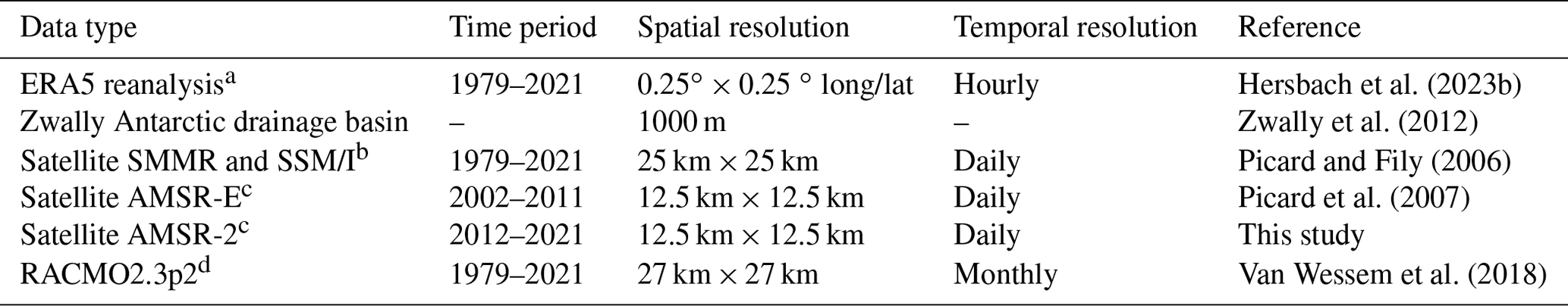
^a The 2 m air temperature data are on single level (Hersbach et al., 2023b). ^b Satellite local acquisition times over Antarctica are around 06:00 and 18:00. ^c Satellite local acquisition times over Antarctica are around 00:00 (descending) and 12:00 (ascending). ^d RACMO2.3p2 surface melt simulations.

The dataset we use in this study is the ECMWF ERA5 reanalysis (Hersbach et al., 2023b) (Table 1). It has hourly data for three-dimensional (pressure level) atmospheric fields (Hersbach et al., 2023a) and on a single level for the atmosphere and land surface (Hersbach et al., 2023b). It replaced the previous ECMWF reanalysis product ERA-Interim in 2019 (Hersbach et al., 2020), and has become the new state-of-the-art ECMWF reanalysis product for global and Antarctic weather and climate (Hersbach et al., 2020; Gossart et al., 2019).

The particular ERA5 product we use in this study is the hourly 2 m air temperature data, which have been evaluated and used previously for studies in Antarctica (e.g. Gossart et al., 2019; Tetzner et al., 2019; Zhu et al., 2021). Assessments have shown that ERA5 near-surface (or 2 m) air temperature data are a robust tool for exploring the Antarctic climate (e.g. Gossart et al., 2019; Zhu et al., 2021). ERA5 performs better at representing near-surface temperature than its predecessors, the Climate Forecast System Reanalysis (CFSR), and the Modern-Era Retrospective Analysis for Research and Applications, version 2 (MERRA-2; Gossart et al., 2019). It is continuously being updated and is one of the most state-of-the-art reanalysis datasets available. However, compared to 48 automatic weather station (AWS) observations, it is reported to have a cold bias over the entire continent apart from the winter months (June–July–August; Zhu et al., 2021). This cold bias is reported at 0.34 ^∘C annually and at 1.06 ^∘C during December–January–February (DJF; Zhu et al., 2021).

2.2 Satellite data

The number of melt days retrieved from the satellite observations is used to parameterize the threshold temperature (T₀) for the PDD model. We use the 42-year daily (once every 2 d before 1988) satellite Antarctic surface melt dataset produced by Picard and Fily (2006) (Table 1). The dataset contains daily estimates as a binary of melt or no-melt on a 25 km × 25 km southern polar stereographic grid. The dataset is obtained by applying the melt detecting algorithm (Torinesi et al., 2003; Picard and Fily, 2006) to detect the presence of surface liquid water on the Scanning Multichannel Microwave Radiometer (SMMR) and three Special Sensor Microwave Imager (SSM/I) observed passive-microwave data from the National Snow and Ice Data Center (NSIDC; Picard and Fily, 2006). SMMR and SSM/I sensors are carried by sun-synchronous orbit satellites observing Earth at least twice per day (Picard and Fily, 2006). For Antarctica, the local acquisition times are around 06:00 and 18:00. The brightness temperature is the daily average of all the passes (those around 06:00 and those around 18:00). There is a reported data gap longer than 1 month during the period from December 1987 to January 1988 (Torinesi et al., 2003; Johnson et al., 2022), and we find additional missing data during the prolonged summer (from November to March) in 1986/1987 (13 d), 1987/1988 (44 d), 1988/1989 (8 d) and 1991/1992 (9 d), which are significantly longer than the length of the missing data period of the remaining 38 years (0 or 1 d, Fig. A1 in Appendix A). We therefore omit those periods from our comparison to the satellite estimates.

We also use a more recently developed satellite melt day dataset which uses a similar algorithm as Torinesi et al. (2003) and Picard and Fily (2006) used for the Advanced Microwave Scanning Radiometer on the Earth Observation Satellite (AMSR-E) and the Advanced Microwave Scanning Radiometer 2 (AMSR-2) observed passive-microwave data from the Japan Aerospace Exploration Agency (JAXA, Table 1). This dataset is on a 12.5 km × 12.5 km southern polar stereographic grid. It has twice-daily observations over Antarctica covering 2002 to 2011 (AMSR-E) and 2012 to 2021 (AMSR-2, Table 1). These sensors have a local acquisition time over Antarctica of around 00:00 (descending) and 12:00 (ascending).

2.3 Regional climate model SEB output

To parameterize the DDF for the PDD model, we compare our ERA5 forced numerical experiments to the Antarctic surface melt simulations from RACMO2.3p2 (Van Wessem et al., 2018). RACMO2.3p2 simulates Antarctic surface melt by solving the SEB model which is defined as (Van Wessem et al., 2018):

$$\begin{array}{}\text{(1)}& Q_{\mathrm{M}}={\mathrm{SW}}_{\downarrow }+{\mathrm{SW}}_{\uparrow }+{\mathrm{LW}}_{\downarrow }+{\mathrm{LW}}_{\uparrow }+\mathrm{SHF}+\mathrm{LHF}+G_{\mathrm{s}},\end{array}$$

where Q_M is the energy available for melting, SW_↓ and SW_↑ are the downward and upward shortwave radiative fluxes, LW_↓ and LW_↑ are the downward and upward longwave radiative fluxes, SHF and LHF are the sensible and latent turbulent heat fluxes and G_s is the subsurface conductive heat flux (Van Wessem et al., 2018).

RACMO2.3p2 Antarctic surface melt simulations used here cover the time period from January 1979 to February 2021 with monthly temporal resolution and 27 km × 27 km spatial resolution (Table 1).

2.4 Interpolation and research domain

The spatially coarsest dataset used in this study is the ERA5 reanalysis data, which are in 0.25^∘ longitude × 0.25^∘ latitude geographic coordinates (Table 1). For consistency with the other data we analyse, we use the southern polar stereographic coordinates instead of the geographic coordinates. We use the Climate Data Operators (CDO; Schulzweida, 2021) to bilinearly remap ERA5 reanalysis data from longitude–latitude geographic coordinates to NSIDC Sea Ice Polar Stereographic South Projected Coordinate System (NSIDC, 2022) (hereafter “polar stereographic grid”). We use a spatial resolution of 30 km, minimizing the number of missing pixels and maximizing the resolution. For consistency, we also use CDO to remap all data products used in this study (Table 1) to the same 30 km × 30 km polar stereographic grid. The research domain is shown in Fig. 1.

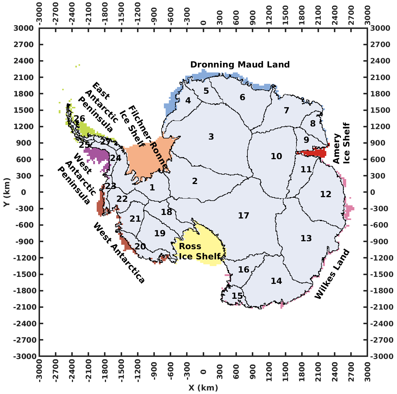
Figure 1 The research domain and 27 Antarctic drainage basins (Zwally et al., 2012) used in this study.

3 Methods

3.1 PDD model

Using an empirical relationship between air temperature and melt, temperature index models are the most commonly used method for assessing surface melt of ice and snow due to their simplicity as they are only meteorologically forced by the air temperature (Hock, 2005). Not only does the simplicity of the approach enable fast run times and require low computational resources, but the air temperature input data are also much easier to obtain than the full inputs (e.g. radiation fluxes, temperature, wind speed, humidity, ice/snow density and surface roughness (van den Broeke et al., 2010)) required by the SEB model. If appropriately parameterized, the temperature index approach offers accurate performance (Ohmura, 2001) and provides a robust surface melt representation. However, because of the temperature dependency, the robustness of the temperature index approach is therefore attributed to the temperature–melt correlation.

The PDD model calculates the water equivalent of surface snow melt (M, $\mathrm{mm}\mathrm{w}.\mathrm{e}.$). It integrates the near-surface air temperatures above a predefined threshold, which are multiplied by the empirical DDF ($\mathrm{mm}\mathrm{w}.\mathrm{e}.{}^{\circ }{\mathrm{C}}^{-\mathrm{1}}{\mathrm{d}}^{-\mathrm{1}}$; e.g. Hock, 2005). The adjusted PDD model we use in this study can be written as

$$\begin{array}{}\text{(2)}& \begin{array}{rl}\sum _{i=\mathrm{1}}^{\mathrm{day}}M& ={\displaystyle \frac{\mathrm{1}}{\mathrm{24}}}\mathrm{DDF}\sum _{i=\mathrm{1}}^{\mathrm{day}}\sum _{j=\mathrm{1}}^{\mathrm{24}}{T}^{\star }\\ & T^{\star }=\left\{\begin{array}{ll}T-T_{\mathrm{0}}& \text{if}T-T_{\mathrm{0}}>\mathrm{0}\\ \mathrm{0}& \text{otherwise}\end{array}\right.,\end{array}\end{array}$$

where T is the hourly temperature and T₀ is the threshold temperature.

3.2 Model parameterization

3.2.1 Threshold temperature T₀

To parameterize the threshold temperature (T₀) for our PDD model, we firstly focus on the binary melt/no-melt signal. We use the ERA5 2 m air temperature data to force the model and run 151 numerical experiments for T₀ ranging from −10.0 to +5.0 ^∘C with a 0.1 ^∘C interval. We define a melt day (MD^⋆) as a day in which the daily input of the ERA5 2 m air temperature (T) exceeds T₀. Note that T is either the daily mean of 06:00 and 18:00 or the daily mean of 00:00 and 12:00 depending on the satellite estimates we compare (detailed in the paragraph below). In each T₀ experiment, we calculate the total number of melt days from 1 April of that year to 31 March of the following year as the “annual number of melt days”. The modified Eq. (2) can be written as

$$\begin{array}{}\text{(3)}& \begin{array}{rl}\text{Annual number of melt days}& =\sum _{i=t_{\mathrm{1}}}^{t_{\mathrm{2}}}{\mathrm{MD}}^{\star }\\ & t_{\mathrm{1}}=\mathrm{1}\mathrm{April}\mathrm{Year}\\ & t_{\mathrm{2}}=\mathrm{31}\mathrm{March}(\mathrm{Year}+\mathrm{1})\\ & {\mathrm{MD}}^{\star }=\left\{\begin{array}{ll}\mathrm{1}& \text{if}T-T_{\mathrm{0}}>\mathrm{0}\\ \mathrm{0}& \text{otherwise}\end{array}\right.\end{array}.\end{array}$$

Because the satellite melt day product of SMMR and SSM/I (Table 1) is retrieved from the local acquisition times at around 06:00 and 18:00, we compute the mean of 06:00 and 18:00 ERA5 2 m air temperature data for the input T for the PDD model (Eq. 3). For the satellite product from AMSR-E and AMSR-2 (Table 1), we compute the mean of 00:00 and 12:00 ERA5 2 m air temperature data as of their local acquisition times. Next, we calculate the result of Eq. (3) for each T₀ experiment.

In order to obtain the optimal T₀, we calculate the root mean square error (RMSE) between the time series of the annual number of melt days for the satellite estimates and the model experiments in the overlapping years. As we treat each computing cell individually, all calculations are carried out on each cell independently in each iteration (T₀ experiment). Although these three satellite products have different time periods (Table 1), we assume their comparability as these satellite products are derived from the same algorithm and threshold (Picard and Fily, 2006). Therefore, we calculate the mean of RMSE between three satellite estimates for each cell. Finally, we define the optimal T₀ of each computing cell, where the T₀ experiment has the minimal RMSE. If there are multiple T₀ experiments that have same minimal RMSE for their computing cell, we calculate the mean of those T₀ as the optimal T₀ (this only happens on the cells that have very few melt days).

3.2.2 Degree-day factor, DDF

The DDF is a scaling parameter that controls the meltwater production and is related to all terms of the SEB (Hock, 2005). To parameterize the DDF for our PDD model, we substitute the optimal T₀ found in Sect. 3.2.1 into the Eq. (2), and run a series of numerical experiments forced by the hourly ERA5 2 m air temperature data: we firstly set the DDF to 1 $\mathrm{mm}\mathrm{w}.\mathrm{e}.{}^{\circ }{\mathrm{C}}^{-\mathrm{1}}{\mathrm{d}}^{-\mathrm{1}}$; then we iterate 291 times with 0.1 $\mathrm{mm}\mathrm{w}.\mathrm{e}.{}^{\circ }{\mathrm{C}}^{-\mathrm{1}}{\mathrm{d}}^{-\mathrm{1}}$ increments.

In order to determine the optimal DDF, we repeat the calculations for the RMSE between the annual melt amount calculated in each DDF experiment and the melt amount from RACMO2.3p2 simulations for each computing cell. Similarly, we define the optimal DDF where the experiment has the minimal RMSE for each computing cell. If there are multiple DDF experiments that have the same minimal RMSE for their computing cell, we calculate the mean of these DDF as the optimal DDF (this only happened for the cells with very low melt amounts).

3.3 Model evaluation

3.3.1 Goodness-of-fit testing

Limited by the duration of the satellite era and reanalysis data, the time series of annual data for each computing cell is no larger than 45 years with non-normality. We use the two-sample Kolmogorov–Smirnov test (hereafter, two-sample KS test) to evaluate the dissimilarity between the PDD results and RACMO2.3p2 melt volume outputs at a confidence level of 5 %. We define a “same distribution cell” as a cell with no statistically significant evidence from the two-sample KS test for the rejection of the null hypothesis (that the two samples are from the same continuous distribution).

3.3.2 K-fold cross-validation

We consider the spatial variability in PDD parameters by parameterizating the model in each computing cell for the whole time period. However, this does not allow us to explore the variability in the PDD parameters in a temporal sense, as Ismail et al. (2023) suggest that the temporal variability in DDF should also be considered. Due to the short period of the satellite-era and the scarcity of in situ Antarctic surface melt data (Gossart et al., 2019), our PDD model is parameterized and evaluated using the same dataset covering the past 4 decades.

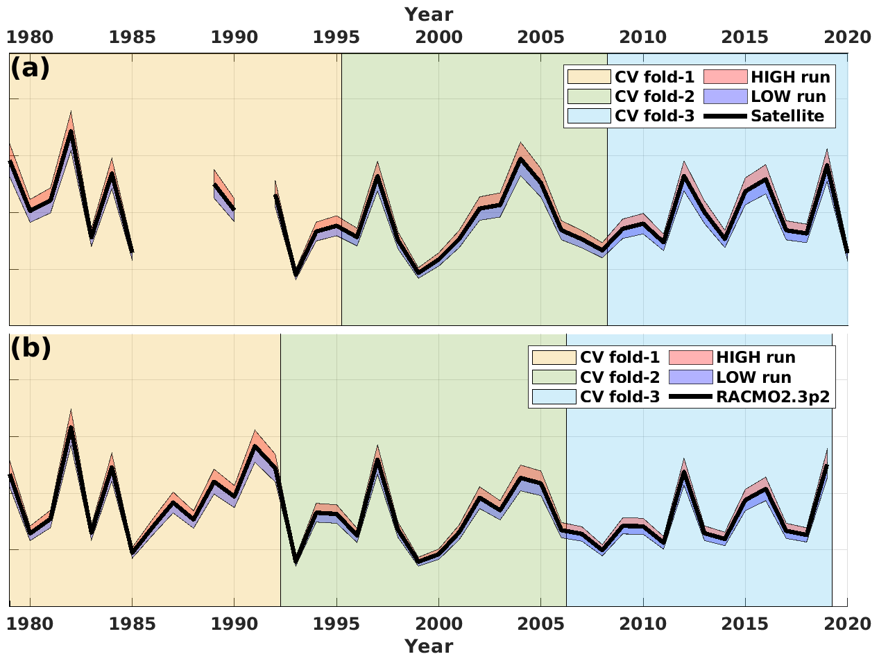
Figure 2 Schematic overview of the time periods for each CV folders and the HIGH/LOW sensitivity experiments. Panel (a) is for satellite estimates and PDD melt day calculations. Panel (b) is for RACMO2.3p2 simulations and PDD melt amount calculations.

Table 2 Periods of training and testing folds for the T₀ and DDF three-fold cross-validation respectively.

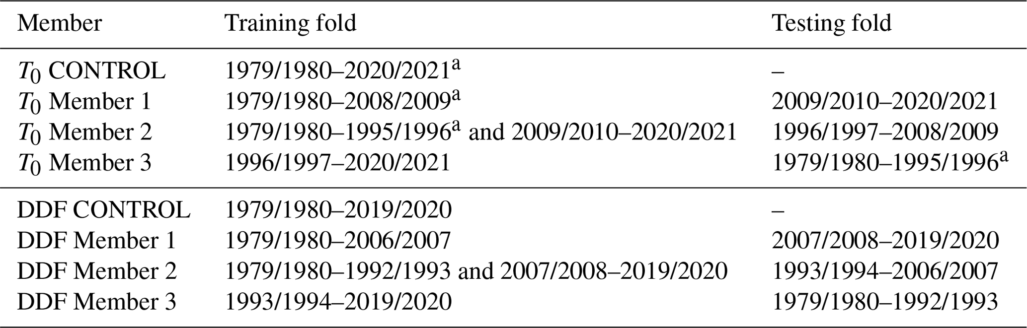
^a periods of 1986/1987 to 1988/1989 and 1991/1992 are omitted.

To therefore assess the temporal dependency of the PDD parameters, we perform an adjusted three-fold cross-validation (hereafter 3-fold CV). The satellite melt occurrence estimates used in this study cover 38 years (four years have been omitted). Therefore, we sequentially divide the satellite estimates into two 13-year folds and one 12-year fold (Fig. 2a and Table 2). Note that in Sect. 3.2.1, we calculate the RMSE between the PDD and three satellite estimates in their overlapping period respectively and calculate the mean of these three RMSE. However, the second fold has actually only 7 years of overlap between the SMMR and SSM/I sensors and the AMSR-E sensor. Here, we firstly calculate the mean of satellite estimates between their overlapping periods prior to the 3-fold CV and then we perform the 3-fold CV. The 3-fold CV has three independent members. In Member 1, we take the first and second fold to parameterize the PDD model and test the model on the third fold. In Member 2, we take the first and third fold to parameterize the PDD model and test the model on the second fold. In Member 3, we take the second and third fold to parameterize the PDD model and test the model on the first fold. Similarly, we repeat the calculations for RACMO2.3p2 surface melt amount but the folds are divided into two 14-year folds and one 13-year fold (Fig. 2b and Table 2).

3.3.3 Sensitivity experiments

Although RACMO2.3p2 is suggested to be one of the best models for reconstructing Antarctic climate, a cold bias of −0.51 K for the near-surface temperatures is also reported (Mottram et al., 2021). However, it is unclear how much this cold bias influences the output of RACMO2.3p2 snowmelt simulations, at least on the spatial scale. Satellite estimates are more direct products for Antarctic surface melt. However, biases in satellite products are likely due to the inconsistency in the characteristics of satellite sensors caused by frequent equipment replacements, which occurred four times in the period 1979–2005 (Picard and Fily, 2006; Picard et al., 2007).

To explore the sensitivity of PDD parameters and model outputs to biases in both the satellite and RACMO2.3p2 products, we perform two sensitivity experiments. In the first sensitivity experiment, we explore the response of T₀ and the PDD melt day and cumulative melting surface (CMS) outputs to perturbations in satellite estimates. The CMS, also known as a melt index (e.g. Trusel et al., 2012), is calculated by multiplying the cell area (km²) by the total annual melt days (d) in that same cell (Trusel et al., 2012). We increase/decrease (HIGH/LOW run) satellite CMS estimates by 10 % (Fig. 2a) for each grid cell; then we repeat the T₀ parameterization as described in Sect. 3.2.1 respectively. In the second sensitivity experiment, we explore the sensitivity of the DDF and the PDD melt amount outputs to perturbations in RACMO2.3p2 melt estimates. We increase/decrease (HIGH/LOW run) RACMO2.3p2 melt estimates by 10 % (Fig. 2b) for each grid cell; we then repeat the DDF parameterization as described in Sect. 3.2.2 respectively. Note that in the context of the sensitivity experiments, our optimal parameterization of T₀ and DDF in Sect. 3.2.1 and 3.2.2 constitutes our CONTROL run.

To assess the applicability of our PDD model in simulating melt under warmer climate scenarios, we conduct temperature–melt sensitivity experiments. To do this, we add constant temperature perturbations of +1, +2, +3, +4 and +5 ^∘C to the whole 43-year (1979/1980 to 2021/2022) ERA5 2 m air temperature field to force our PDD model.

4 Results and discussion

4.1 Optimal PDD parameters

Figure 3a shows the spatial distribution of the optimal T₀ values selected through 151 T₀ experiments conducted on each computing cell based on the minimal RMSE criterion. The mean of all optimal T₀ is −2.32 ^∘C. The majority of cells have a negative T₀, indicating that using T₀=0 ^∘C as a melt threshold may substantially underestimate melt events, a finding consistent with other work (Jakobs et al., 2020).

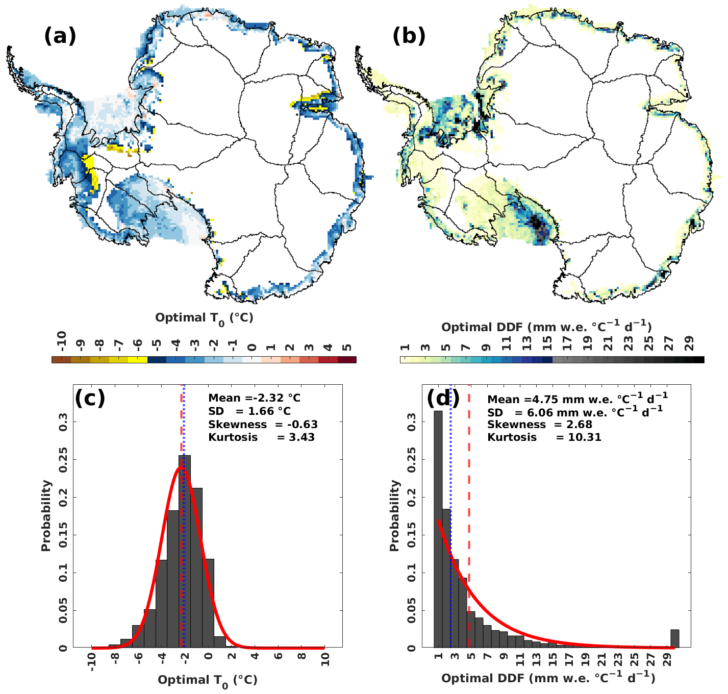
Figure 3 (a) The optimal T₀ (^∘C) of each computing cell. (b) The optimal DDF ($\mathrm{mm}\mathrm{w}.\mathrm{e}.{}^{\circ }{\mathrm{C}}^{-\mathrm{1}}{\mathrm{d}}^{-\mathrm{1}}$) for each computing cell. (c) Probability histogram of the optimal T₀ (^∘C). Red curve is the fitted normal distribution. Vertical dashed red line is the mean of T₀ for all computing cells. Dotted blue line is the median of T₀ for all computing cells. (d) Probability histogram for the optimal DDF ($\mathrm{mm}\mathrm{w}.\mathrm{e}.{}^{\circ }{\mathrm{C}}^{-\mathrm{1}}{\mathrm{d}}^{-\mathrm{1}}$). Red curve is the fitted exponential distribution. Vertical dashed red line is the mean of DDF for all computing cells. Dotted blue line is the median of DDF for all computing cells.

The probability distribution of T₀ across all grid cells is approximately normal (Fig. 3c). There is a small number of cells distributed below −5.5 ^∘C, which is around 1.96 standard deviations lower than the mean (−5.57 ^∘C, Fig. 3c). We highlight these lower-end tail cells in yellow in Fig. 3a. These cells are mainly distributed in two areas. One is the interior boundary of the satellite observational area (Fig. A2 in Appendix A) over the drainage basins (e.g. Basin 1, 9, 21 and 22), which is not surprising as the optimal T₀ values there might not be significant given the non-statistically significant (p≥0.05) temperature–melt correlation over those cells (Fig. B1 in Appendix B). The other area is the central Amery Ice Shelf (Fig. 3a). We speculate that this feature may be related to the presence of local rocks (e.g. Fricker et al., 2021; Spergel et al., 2021) or it could be a result of frequent surface melt events over the central Amery Ice Shelf (as suggested by the low T₀ value), which are likely to have a low intensity (as indicated by the low DDF value).

Figure 3b shows the spatial map of the optimal DDFs identified for each computing cell. We show that a large number of DDFs with relatively low magnitude (from 1 to 4.5 $\mathrm{mm}\mathrm{w}.\mathrm{e}.{}^{\circ }{\mathrm{C}}^{-\mathrm{1}}{\mathrm{d}}^{-\mathrm{1}}$, coloured light yellow) are distributed over ice shelves other than the Ross Ice Shelf and Filchner–Ronne Ice Shelf (Fig. 3b). We highlight DDFs larger than 15.5 $\mathrm{mm}\mathrm{w}.\mathrm{e}.{}^{\circ }{\mathrm{C}}^{-\mathrm{1}}{\mathrm{d}}^{-\mathrm{1}}$ in red in Fig. 3b. Although the magnitude of the DDF over the cells located in the west Ross Ice Shelf and south-east Filchner–Ronne Ice Shelf may exceed the upper boundary (30 $\mathrm{mm}\mathrm{w}.\mathrm{e}.{}^{\circ }{\mathrm{C}}^{-\mathrm{1}}{\mathrm{d}}^{-\mathrm{1}}$) of our DDF experiments that we heuristically defined in Sect. 3.2.2, we do not expand the upper boundary of the DDF or perform more DDF experiments. This is because (1) the temperature–melt correlations over those cells are not statistically significant (p≥0.05, Fig. B1), and therefore the PDD model which is based on the temperature–melt relationship for these cells may not be significant; (2) the total number of these cells is less than 5 % of the total number of the computing cells (Fig. 3d); (3) surface melting in these cells is negligible under present-day conditions and even remains negligible in RCP8.5 2100 future projection (Trusel et al., 2015); (4) these parameters are empirically defined by minimizing the RMSE between PDD experiments and satellite estimates/RACMO2.3p2 simulations, which means the optimal parameters are likely less robust over cells where melt is rare. Figure 3d summarizes the statistics of DDFs. The probability distribution of the DDFs is asymmetrical and strongly right-skewed (Fig. 3d).

We also use the same method and data to parameterize a spatially uniform PDD (hereafter, “uni-PDD”) model (one T₀ and DDF for all computing cells, Appendix C). For convenience, we name the grid-cell-level spatially distributed PDD “dist-PDD”. The optimal T₀ for uni-PDD is −2.6 ^∘C and the optimal DDF is 1.9 $\mathrm{mm}\mathrm{w}.\mathrm{e}.{}^{\circ }{\mathrm{C}}^{-\mathrm{1}}{\mathrm{d}}^{-\mathrm{1}}$ (Fig. C1 in Appendix C).

4.2 Model evaluation

4.2.1 Goodness-of-fit

We evaluate the parameterized dist-PDD and uni-PDD model outputs (melt day and melt amount) for each computing cell by testing the statistical significance of the similarity between the satellite estimates or RACMO2.3p2 simulations and the dist-PDD/uni-PDD model-derived empirical distribution functions. Figure 4 shows the two-sample KS test results for each computing cell. The dist-PDD model improves the proportion of cells with the same distribution of melt days and melt amount from 60.04 %/65.94 % to 86.07 %/71.16 % respectively compared to the uni-PDD model. Overall, the dist-PDD model shows good agreement with the satellite estimates and RACMO2.3p2 simulations in estimating both the annual total of melt days and melt amount (Fig. 4c and d). Our dist-PDD model is particularly well suited for estimating surface melt over the ice shelves in the Antarctic Peninsula, while cells located in other ice shelves, such as the Filchner–Ronne Ice Shelf, ice shelves in Dronning Maud Land, Amery Ice Shelf and Ross Ice Shelf, do not perform as well for both the surface melt days and amount (Fig. 4c and d). It is especially encouraging that the PDD model performs well in the Antarctic Peninsula given the fact that it is the region of Antarctica experiencing most intense surface melting both at the present (Trusel et al., 2013; Johnson et al., 2022) and in future projections (Trusel et al., 2015).

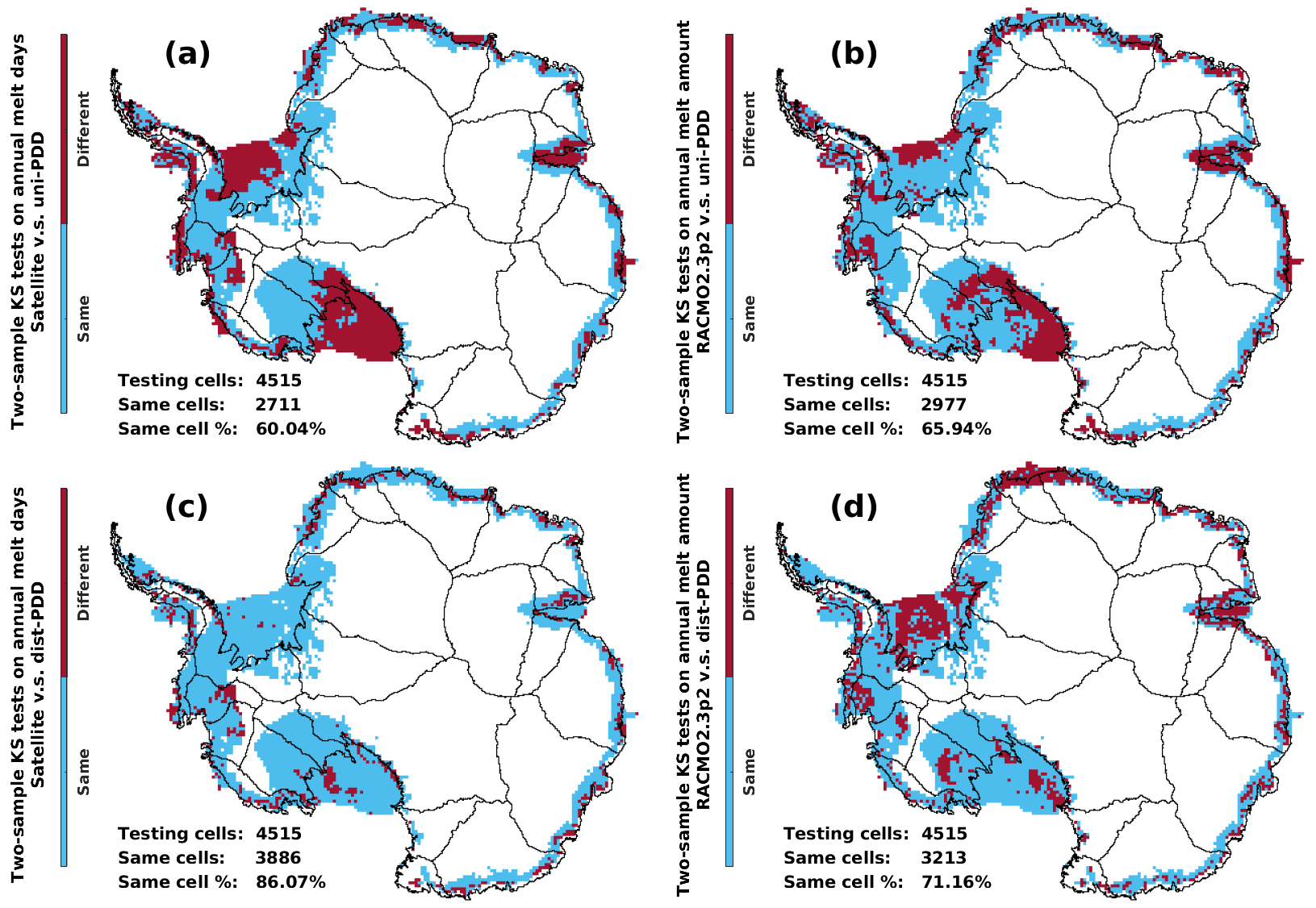
Figure 4 The two-sample KS test results. The two-sample KS tests are performed individually for each of the 4515 computing cells. The test result “Same” means the tested cell is a “same distribution cell” where there is no statistically significant evidence for the rejection of the null hypothesis that the testing two samples are from the same continuous distribution (Sect. 3.3.1). Otherwise, the cell is a “different distribution cell” (“Different”). Panels (c) and (a): the two-sample KS test results for testing the annual number of melt days between the satellite estimates and the dist-PDD/uni-PDD model outputs. Panels (d) and (b): the two-sample KS test results for testing the annual melt amount between RACMO2.3p2 simulations and the dist-PDD/uni-PDD model outputs.

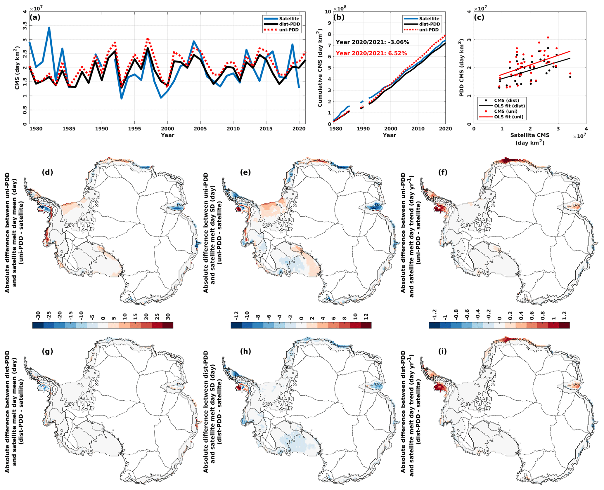
Figure 5 (a) Time series for the cumulative melting surface (CMS; d km²) for satellite estimates during the period from 1979/1980 to 2020/2021 (with 1986/1987 to 1988/1989 and 1991/1992 omitted), and for dist-PDD/uni-PDD outputs during the period from 1979/1980 to 2021/2022. (b) CMS for satellite estimates and dist-PDD/uni-PDD outputs from 1979/1980 to 2020/2021 (with 1986/1987 to 1988/1989 and 1991/1992 omitted). (c) scatter plot and ordinary least squares (OLS) fit between satellite CMS and dist-PDD/uni-PDD CMS. Panels (d) to (i): absolute differences between mean, standard deviation (SD) and trend of dist-PDD/uni-PDD outputs and satellite estimates of the annual melt days. Mean, SD and trend for the dist-PDD/uni-PDD outputs and satellite estimates are calculated over the period from 1979/1980 to 2020/2021 (with 1986/1987 to 1988/1989 and 1991/1992 omitted) respectively. Note that for all panels the satellite estimates from 2002/2003 to 2010/2011 are the average of the SMMR and SSM/I sensors and the AMSR-E sensor. The satellite estimates from 2012/2013 to 2020/2021 are the average of the SMMR and SSM/I sensors and the AMSR-2 sensor.

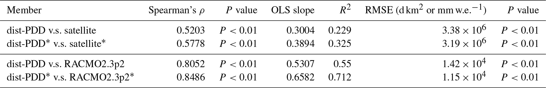
Table 3 Summary of the statistics for Fig. 5c. The Spearman's ρ and P value for dist-PDD/uni-PDD CMS with the satellite CMS. Slope, R², RMSE and P value for the ordinary least squares (OLS) fit between dist-PDD/uni-PDD CMS and satellite CMS. Note that the satellite estimates from 2002/2003 to 2010/2011 are the average the SMMR and SSM/I sensors and the AMSR-E sensor. The satellite estimates from 2012/2013 to 2020/2021 are the average the SMMR and SSM/I sensors and the AMSR-2 sensor. All the statistics are calculated over the period from 1979/1980 to 2020/2021 (with 1986/1987 to 1988/1989 and 1991/1992 omitted).

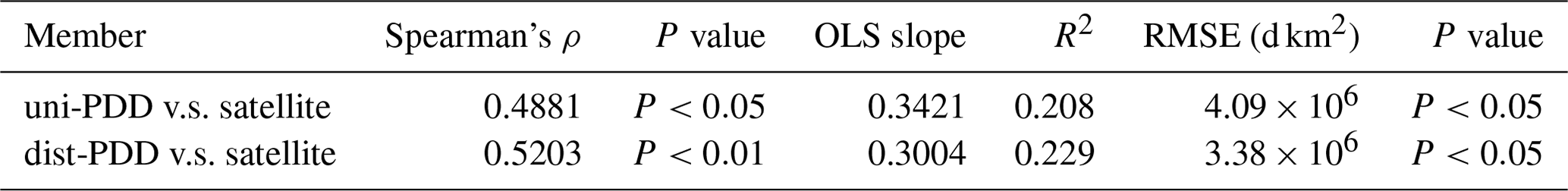
Next, we evaluate the parameterized dist-PDD/uni-PDD model outputs for the whole of Antarctica. Firstly, we evaluate the parameterized optimal T₀ and its related dist-PDD/uni-PDD outputs on the surface melt day. To do this, we calculate the CMS (d km²) for satellite estimates and dist-PDD/uni-PDD outputs respectively. We show that in Fig. 5a that the dist-PDD and satellite CMS time series are generally in good agreement regarding both the amplitude and the temporal variability, apart from a small number of years including from 1979/1980 to 1982/1983, the year 2014/2015, the year 2016/2017 and the year 2019/2020. Although there is a dist-PDD underestimation of CMS for the first decade (1980 to 1990), the CMS of dist-PDD at the end of the 38-year period is in good agreement with the CMS of satellite estimates (−3.06 % PDD CMS underestimation compared to the satellite CMS, Fig. 5b). The positive correlation between the satellite CMS and the dist-PDD CMS is strongly statistically significant (Spearman's ρ=0.5203, p<0.01, Table 3). The probability histogram for biases between the dist-PDD and satellite CMS also indicates good agreement between the dist-PDD and satellite CMS (Fig. D1 in Appendix D). The biases are distributed symmetrically around the mean, which is approximated to zero (Fig. D1).

Globally, we show that the accuracy of the PDD models in estimating the surface melt days has improved from the uni-PDD model to the dist-PDD model (Table 3 and Fig. 5), and the dist-PDD model has the ability to capture the main spatial patterns of surface melt days when compared to the satellite estimates for a majority of the computing cells (Fig. 5). The computing cells that have relatively large disagreement between the mean annual melt days of dist-PDD outputs and of satellite estimates are mainly located over the ice shelves in the Antarctic Peninsula ($\sim -\mathrm{2.5}$ to −22.5 d), over the Abbot Ice Shelf ($\sim -\mathrm{5.5}$ to −12.5 d over the marine edge and $\sim +\mathrm{2.5}$ to +7.5 d over the interior) and over the Shackleton Ice Shelf ($\sim +\mathrm{7.5}$ to +12.5 d). However, these cells, with large absolute differences, experience frequent surface melt (Fig. D2a and d in Appendix D), meaning that the relative differences in melt are low (Fig. D2g). In addition, these cells only amount to around 5 % of the total computing cells (Fig. D1b), and overall for all computing cells, the mean of the average differences between the dist-PDD and satellite annual melt days is approximately zero (−0.12 d, Fig. D1b). It is not surprising that the dist-PDD model captures the main spatial patterns of melt given the statistically significant positive correlation between surface melt and 2 m air temperature in most of the Antarctic ice shelf and coastal cells used in the calculations (Fig. B1).

The computing cells that have relatively large absolute differences in SD are mainly located over the Wilkins Ice Shelf ($\sim +\mathrm{4.5}$ to +13.5 d) and over the south of Larsen C Ice Shelf ($\sim -\mathrm{7.5}$ to −10.5 d). Similar to the cells that have relatively large absolute differences in their means, the relative differences are low (Fig. D2h) and these cells amount only to a negligible proportion (less than 5 %) of the total number of the computing cells (Fig. D1b). However, around 20 % of the computing cells have −1 to −3 d SD biases (Fig. D1b), spatially distributed widely over the eastern Ross Ice Shelf, West Antarctica drainage basins 18 and 19, the Abbot Ice Shelf, ice shelves in Dronning Maud Land and the Amery Ice Shelf (Fig. 5h). The biases in trend are not symmetrical about zero, both shown by the dominant area of red colour (all ice shelves in the Antarctic Peninsula, almost all ice shelves in Dronning Maud Land and nearly the whole Amery Ice Shelf) to blue (some computing cells over the Wilkes Land) in Fig. 5i and a slightly right-skewed probability histogram of trend biases with a positive mean (+0.04 d yr⁻¹, Fig. D1c).

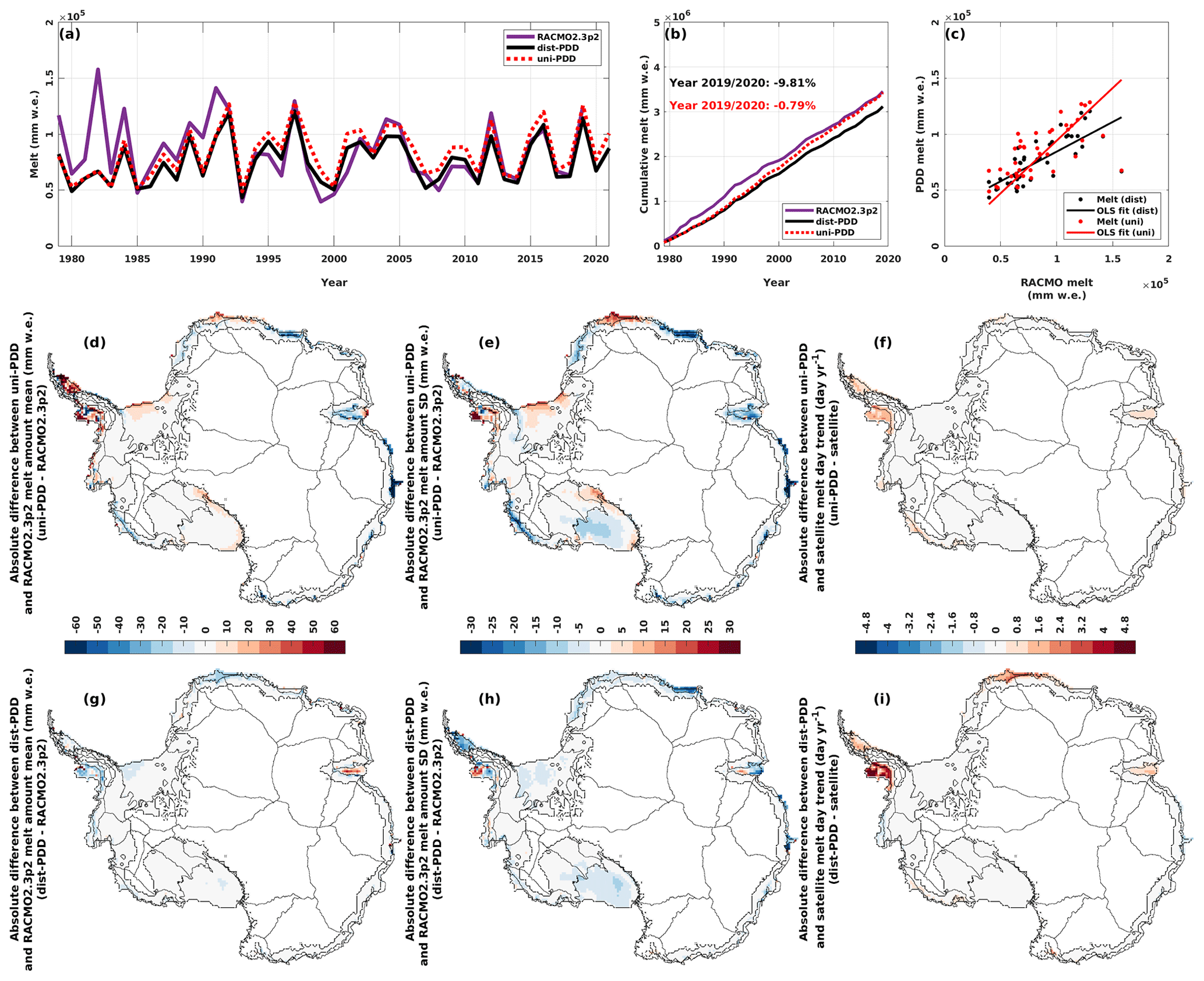
Figure 6 (a) Time series for the annual melt amount (mm w.e.) for RACMO2.3p2 simulations during the period from 1979/1980 to 2019/2020 and for dist-PDD/uni-PDD outputs during the period from 1979/1980 to 2021/2022. (b) Cumulative annual melt amount for RACMO2.3p2 simulations and dist-PDD/uni-PDD outputs from 1979/1980 to 2019/2020. (c) Scatter plot and ordinary least squares (OLS) fit between satellite annual melt amount and dist-PDD/uni-PDD annual melt amount. Panels (d) to (i): absolute differences between mean, standard deviation (SD) and trend of dist-PDD/uni-PDD outputs and RACMO2.3p2 simulations on the annual melt amount. Mean, SD and trend for the dist-PDD/uni-PDD outputs and satellite estimates are calculated over the period from 1979/1980 to 2019/2020 respectively.

Table 4 Summary of the statistics for Fig. 6c. The Spearman's ρ and P value for dist-PDD/uni-PDD melt amount with the RACMO2.3p2 melt amount. Slope, R², RMSE and P value for the ordinary least squares (OLS) fit between dist-PDD/uni-PDD melt amount and RACMO2.3p2 melt amount. All the statistics are calculated over the period from 1979/1980 to 2019/2020.

Secondly, we evaluate the parameterized optimal DDF and the simulated surface melt amount. Similar to the negative biases between the dist-PDD and the satellite estimates for the CMS for the period from 1979/1980 to 1982/1983 (Fig. 5a), the negative biases of dist-PDD against RACMO2.3p2 are also present when compared to the annual melt amount for 1982/1983 (Fig. 6a). The abnormally extensive melt in 1982/1983 has been reported by previous studies (Zwally and Fiegles, 1994; Liu et al., 2006; Johnson et al., 2022). It is suggested to be driven by the Southern Annular Mode (SAM) because of an inverse relationship between the number of melt days in Dronning Maud Land and the southward migration of the southern westerly winds (Johnson et al., 2022). The disagreement of the dist-PDD model for this extensive melt event is most likely explained by the absence of any substantial temperature anomaly in the ERA5 2 m temperature input (Fig. E1 in Appendix E) because of the temperature dependency of the PDD model (Eq. 2) and the temperature–melt relationship (Fig. B1). It could also partly be explained by the fact that the dist-PDD parameters were defined based on fitting multi-decadal time series between dist-PDD experiments and satellite/RACMO2.3p2 (Sect. 3.2.1 and 3.2.2), meaning that some inter-/intra-annual signals may not be fully captured.

Apart from the 1982/1983 event, other negative biases from dist-PDD are also evident in the period from 1991/1992 to 1992/1993 (Fig. 6a). However, we cannot compare this dist-PDD melt amount bias period to the dist-PDD CMS bias as the year 1991/1992 is omitted for the entire analysis related to the satellite estimates due to the missing satellite data. Excluding these periods, the time series of annual melt amount of the dist-PDD outputs and RACMO2.3p2 simulations are generally in good agreement, especially after 1992/1993, when the two curves start to overlap (Fig. 6a), while the dist-PDD-satellite CMS values show some disagreement (e.g. 1995/1996, 1999/2000, 2014/2015, 2016/2017 and 2019/2020, Fig. 5a). It is also evident from the statistically significant strong positive correlation (Spearman's ρ=0.8052, p<0.01, Table 4) that the dist-PDD is in good agreement with RACMO2.3p2 annual melt amount. However, the probability histogram of dist-PDD melt biases is slightly left-skewed with a negative mean (−0.08 × 10⁵ mm w.e., Fig. D3 in Appendix D) and the dist-PDD model underestimates around 9.81 % for the 41-year integrated annual melt amount compared to RACMO2.3p2 (Fig. 6b). Nevertheless, this underestimation of the 41-year integrated annual melt amount does not change through the past 4 decades, as we show that in Fig. 6b, the two curves differ in the first decade (i.e. the gap between the two curves is increasing from ∼1980 to ∼1990) and become parallel for the following 3 decades. Although the 41-year integrated annual melt amounts for 2019/2020 between uni-PDD and RACMO2.3p2 show very good agreement (−0.79 %, as shown in Fig. 6b), the two cumulative curves are not parallel. The uni-PDD curve diverges from the RACMO2.3p2 curve for around 15 years and then converges to RACMO2.3p2 for the rest of the time period (as shown in Fig. 6b). This indicates that the uni-PDD model is not sufficiently flexible to accurately estimate surface melt amount.

Figure 6d to i show the spatial maps for the difference between the mean, SD and trend of the dist-PDD/uni-PDD annual melt amount and RACMO2.3p2 mean annual melt amount for the period from 1979/1980 to 2019/2020. The spatial maps for the mean, SD and trend of the dist-PDD/uni-PDD annual melt amount and RACMO2.3p2 mean annual melt amount for the same period are shown in Fig. D4 in Appendix D. Consistent with the PDD melt day estimates, using the dist-PDD model improves the accuracy of surface melt amount estimation compared to using spatially uniform PDD parameters. As shown in Fig. 6g, h and i, the differences over most of the computing cells are equal to or close to zero, which is similar to the spatial difference maps between the dist-PDD outputs and satellite estimates shown in Fig. 5g, h and i. This indicates that the dist-PDD model has the ability to capture the main spatial patterns of both the surface melt days and amount, when compared to the satellite estimates and RACMO2.3p2 simulations, for the majority of the computing cells. Less than 5 % of the total number of all computing cells are 15 mm w.e. below or above the bias in the mean (Fig. 6g). These cells are distributed over the western Antarctic Peninsula, ice shelves in Dronning Maud Land and the Amery Ice Shelf. For the disagreement in SD, around 10 % of the total number of the computing cells are biased by −5 to −15 mm w.e. (Fig. 6h). The computing cells that have relatively large disagreement in SD are spatially distributed over the Antarctic Peninsula, ice shelves in eastern Dronning Maud Land, the Amery Ice Shelf and ice shelves in western Wilkes Land (Fig. 6h). The bias in trends between the dist-PDD and RACMO2.3p2 annual melt amount is similar to the bias in trends between the dist-PDD and satellite annual melt days, as they both have the same positive spatial bias patterns (Antarctic Peninsula, Dronning Maud Land and Amery Ice Shelf, Figs. 5i and 6i) and similar right-skewed probability histograms with positive means (Figs. D1c and D3c). This could be explained by other players driving surface melting, such as the SAM (Torinesi et al., 2003; Tedesco and Monaghan, 2009; Johnson et al., 2022), which explains ∼11 %–36 % of the melt day variability (Johnson et al., 2022). However, these biases in trends are a reflection of the trend of the input temperature (Fig. D5 in Appendix D) because of the correlation between air temperature and surface melt (Fig. B1). The disagreement in trends, therefore, is actually between the satellite/RACMO2.3p2 and ERA5 2 m temperature, rather than between the satellite/RACMO2.3p2 and the dist-PDD model itself.

4.2.2 Temporal dependency of the dist-PDD parameters

To evaluate our dist-PDD model in a temporal sense, we perform 3-fold CV for T₀ and DDF (as described in Sect. 3.3.2) respectively.

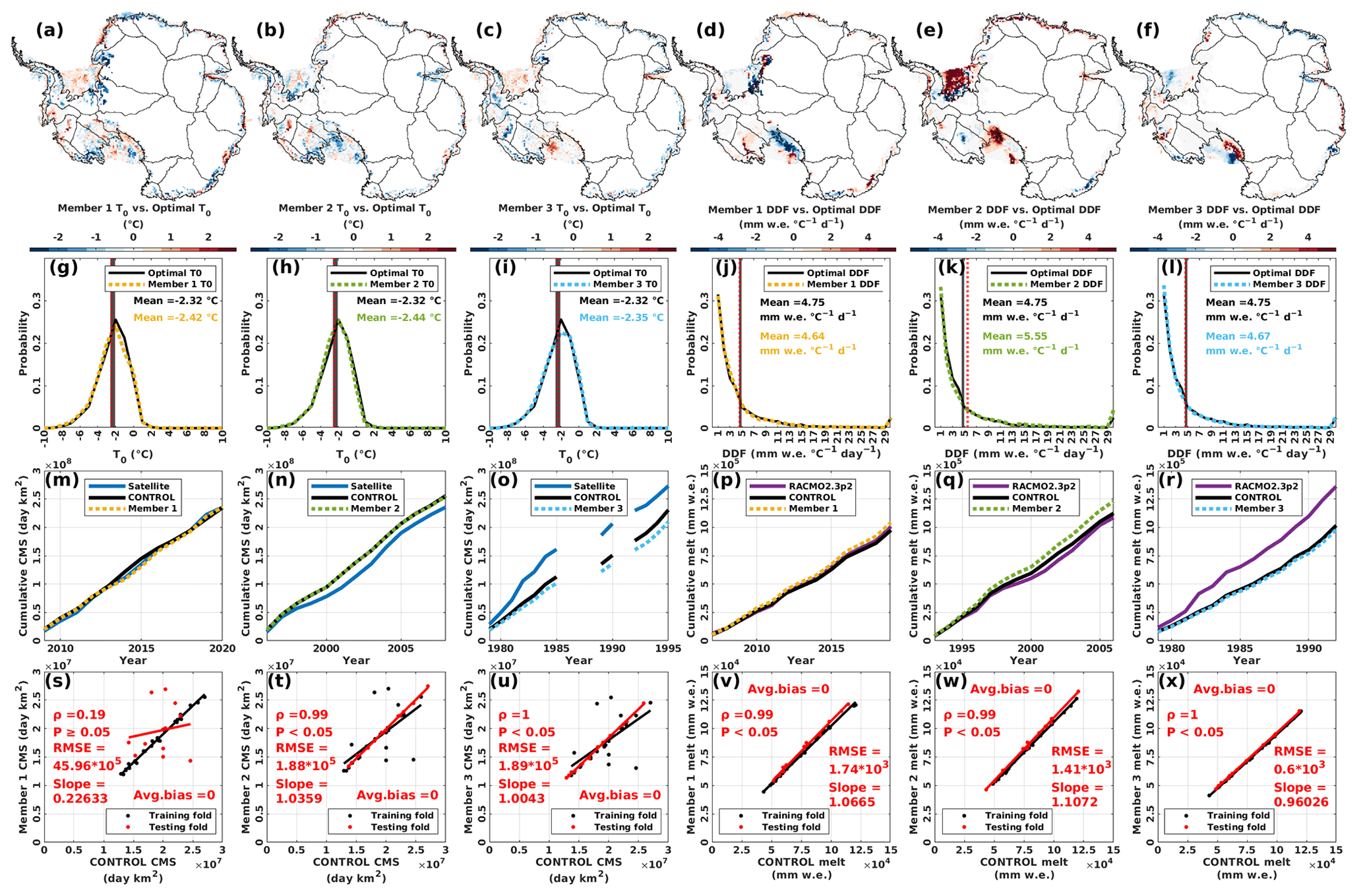
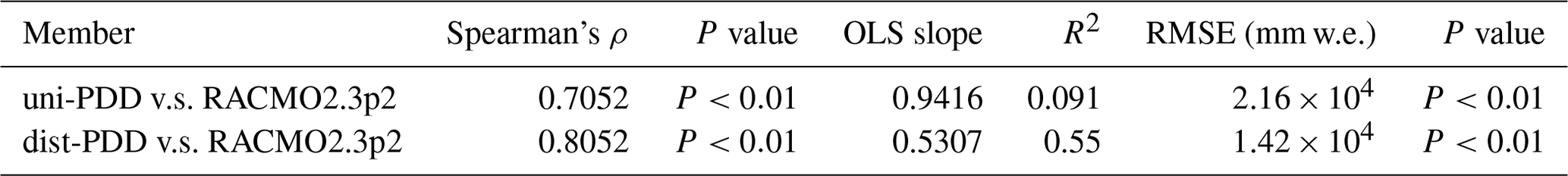
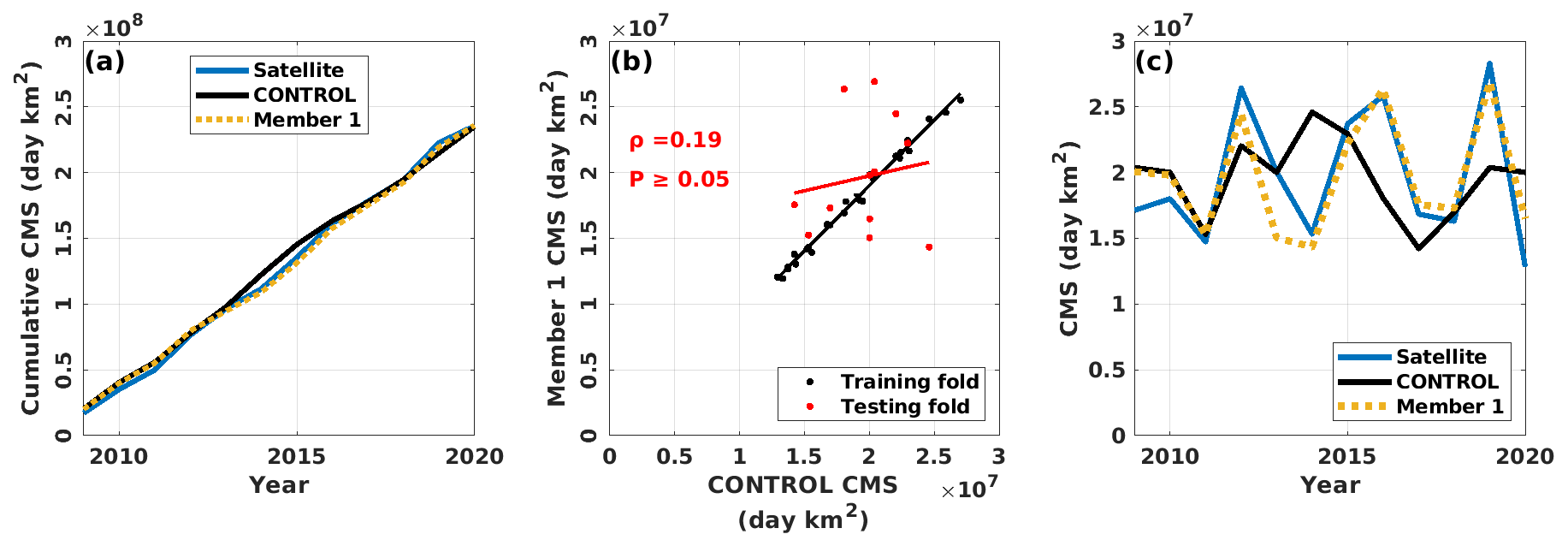
Figure 7 Panels (a) to (f): differences between the T₀/DDF parameterized in each member of the T₀/DDF 3-fold CV and the optimal T₀/DDF respectively. Panels (g) to (l): probability distributions for the T₀/DDF of each T₀/DDF 3-fold CV and the optimal T₀/DDF respectively. Vertical black lines indicate the mean of optimal T₀s/DDFs. Vertical dotted red lines indicate the mean of T₀/DDF for each member respectively. Panels (m) to (r): CMS/annual melt amount for satellite estimates/RACMO2.3p2 simulations, CONTROL (which is the PDD model run with optimal T₀ and DDF) and each member for the period of the testing fold respectively. We calculate the difference in CMS/annual melt amount between each member and the CONTROL, at the end of the testing fold respectively. Panels (s) to (x): scatter plots for the CMS/annual melt amount of each 3-fold CV member against the CONTROL respectively. The Spearman's ρ and its statistical significance, as well and the slope, RMSE and average bias for the OLS fit, for the testing fold between each member and the CONTROL are calculated respectively. This analysis is based on dist-PDD.

Figure 7 shows the results of the 3-fold CV on T₀ and DDF. We show that in Fig. 7a to f that there are changes in the value of T₀ and DDF for a dominant number of the computing cells, depending on the time window (i.e. the training fold) we choose to parameterize the dist-PDD model. Especially for the DDF members, we show conspicuous changes in the values of the DDFs in the computing cells over the western and southern Ross Ice Shelf, the Filchner–Ronne Ice Shelf and coastal basins 2 and 3 (Fig. 7d, e and f), which indicates that a large temporal variability in dist-PDD parameters may exist. However, this indication may not be reliable for the western and southern Ross Ice Shelf and coastal basin 2, given that there is no statistically significant evidence for the temperature–melt relationship (Fig. B1).

Although we show parameter changes associated with the time windows for the dominant number of the computing cells, these changes diminish when we look at the whole population of the parameters in each member (Fig. 7g to l). It is evident that the probability histogram of the optimal parameters and the probability histogram of each member's parameters are closely comparable, with negligible differences between means (excluding DDF Member 2 where the differences between means is relatively larger: +0.8 $\mathrm{mm}\mathrm{w}.\mathrm{e}.{}^{\circ }{\mathrm{C}}^{-\mathrm{1}}{\mathrm{d}}^{-\mathrm{1}}$, Fig. 7k).

Next, we evaluate each member's parameters on the testing fold. Firstly, we calculate the CMS/annual melt amount for the time windows of the testing folds from the dist-PDD models that are parameterized by the training folds for each T₀ and DDF members respectively. Overall, the curves of each member are comparable and overlapping with the CONTROL (Fig. 7m to r), indicating the temporal consistency of our dist-PDD model and the ability of our dist-PDD model in estimating the Antarctic-wide surface melt in terms of the melt occurrence (CMS) and the melt totals (amount) is independent of the time windows chosen for the parameterization. Although the parameters in each computing cells vary through the parameterization time window, the overall performance of the dist-PDD model for all the computing cells as a whole is generally consistent.

Secondly, we calculate the Spearman's ρ and its statistical significance for the testing fold between each member and the CONTROL (Fig. 7s to x). Apart from T₀ Member 1, we show that each member's dist-PDD estimates are significantly (ρ≥0.99, p≤0.05) correlated with the CONTROL dist-PDD estimates (Fig. 7t to x). However, this is not surprising given the comparable probability distributions of parameters and the indistinguishable cumulative curves between each member's dist-PDD and the CONTROL dist-PDD (Fig. 7g to r). The estimates of T₀ Member 1 dist-PDD estimates and dist-PDD CONTROL are strongly correlated with the training fold (black dots in Fig. 7s), which is not surprising as T₀ Member 1 dist-PDD is parameterized by those dist-PDD CONTROL estimates. Estimates of T₀ Member 1 dist-PDD and dist-PDD CONTROL are not significantly correlated (ρ=0.19, p≥0.05) with the testing fold (red dots, Fig. 7s).

To further explore this disagreement in the testing fold, we plot the time series of CMS for satellite estimates, CONTROL estimates and T₀ Member 1 estimates in Fig. F1 in Appendix F. We find that T₀ Member 1 estimates in the testing fold are likely not unrealistic values. Instead, they are in good agreement with the satellite estimates over the testing fold period, as the time series of satellite CMS and Member 1 CMS almost overlap. Therefore the disagreement between T₀ Member 1 estimates and the CONTROL estimates over the testing fold period might explain the disagreement between the satellite estimates and CONTROL estimates as the time series of satellite CMS and Member 1 CMS almost overlap. Although the abilities of Member 1 T₀ and optimal T₀ in capturing the cumulative satellite estimates are robust and indistinguishable (Fig. 7m), the agreement between the time series of Member 1 T₀ and satellite CMS may suggest that T₀ parameterized by the Member 1 training fold (which is the period from 1979/1980 to 2008/2009 with 1986/1987–1988/1989 and 1991/1992 omitted) are more robust in capturing the inter-annual variability in the satellite estimates (for the period from 2009/2010 to 2020/2021) than the optimal T₀ that is parameterized by the full 38-year period. However, the data sample used to parameterize the Member 1 T₀ is only two-thirds the full data length used to estimate the optimal T₀, giving us less confidence in the reliability of the Member 1 T₀s for the full 38-year period.

4.2.3 Sensitivity experiments and implementation in future predictions

Figure 8 shows the result from our sensitivity experiments. We show changes in the dist-PDD parameters associated with the increase (HIGH run, +10 % magnitude of the satellite/RACMO2.3p2 data) and decrease (LOW run, −10 % magnitude of the satellite/RACMO2.3p2 data) in the satellite estimates and RACMO2.3p2 simulations (Fig. 8a to d). It is expected that T₀ decreases/increases with the increase/decrease in the satellite estimates because a decrease in the threshold temperature is expected to increase the occurrence of temperatures above the threshold to produce more melt days, and vice versa. The increase/decrease in RACMO2.3p2 simulations leads to an increase/decrease on the DDFs, which is also expected because T₀ is predefined for the DDF parameterization; thus the sum of the degrees above T₀ becomes invariant. Therefore, as a scaling number, the DDF is expected to increase to amplify the sum of the degrees above T₀ to match the increase in RACMO2.3p2 melt amount simulations, and vice versa.

Figure 8 Panels (a) and (b): difference between T₀ parameterized in the HIGH/LOW experiment and the CONTROL (optimal) T₀. Panels (c) and (d): spatial maps for the difference between the DDF parameterized in the HIGH/LOW experiment and the CONTROL (optimal) DDF. Panels (e) and (g): CMS/annual melt amount for the satellite estimates/RACMO2.3p2 simulations and dist-PDD outputs. Note that the period for (e) is from 1979/1980 to 2020/2021 (with 1986/1987 to 1988/1989 and 1991/1992 omitted). The period for (g) is from 1979/1980 to 2019/2020. The upper and lower boundaries of the semi-transparent shaded areas indicate the HIGH/LOW satellite estimates and the HIGH/LOW dist-PDD outputs. The percentage difference annotated in the bottom-left corner is calculated between the HIGH/LOW and the CONTROL for each variable (by “variable”, we mean satellite melt occurrence data/dist-PDD melt occurrence and amount data/RACMO2.3p2 melt amount data) respectively. Panels (f) and (h): scatter plots and the Spearman’s ρ (with its statistical significance) for dist-PDD outputs and satellite/RACMO2.3p2, from each sensitivity experiment (HIGH, LOW and CONTROL). This analysis is based on dist-PDD.

Figure 8e shows that the dist-PDD model is less sensitive to the low melt scenario than the satellite estimates as the dist-PDD estimates only decrease by 9.78 % for the integrated 38-year CMS, while the satellite estimates decrease by 10 %. Although the dist-PDD model is more sensitive to the high melt scenario than the satellite estimates, where we show that dist-PDD increases by 10.84 % in the 38-year integrated CMS with the 10 % increase in the satellite estimates, this increase in dist-PDD estimates is linear with respect to the increase in satellite estimates and is of the same proportion (Fig. 8e). For the sensitivity experiments on the DDF, we show that the dist-PDD model is less sensitive than RACMO2.3p2 in both the HIGH and LOW melt scenarios. Taken together, the sensitivity of the dist-PDD model is linear (the correlations do not change much across different sensitivity experiments, Fig. 8f and h) and by the same order of magnitude to both the satellite estimates and RACMO2.3p2 simulations, suggesting that our parameterization method is consistent with both the high and low melt scenarios.

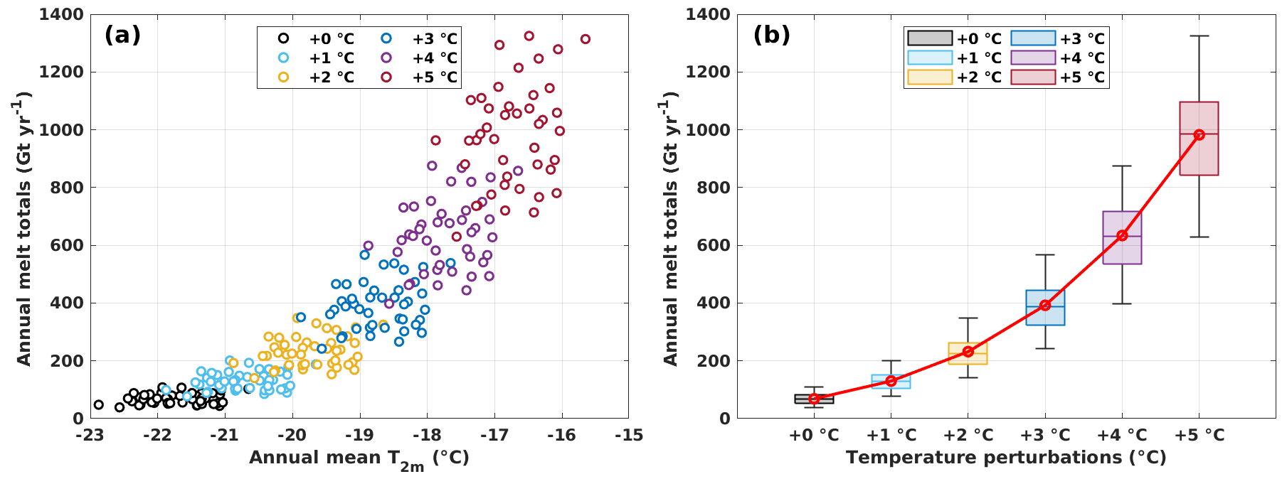
Figure 9 (a) Scatter plot between annual mean 2 m air temperature (T_2m) and Antarctic annual melt totals for each temperature–melt sensitivity experiment for the period from 1979/1980 to 2021/2022. (b) Boxplot of Antarctic annual melt totals for each temperature–melt sensitivity experiment for the period from 1979/1980 to 2021/2022.

Figure 9 shows the results from our temperature–melt sensitivity experiments. We show a nonlinear increase in our dist-PDD estimates of Antarctic surface melt totals as the temperature perturbation gradually rises from +0 to +5 ^∘C. It is not surprising that both the mean and standard deviation increase, given the anticipated nonlinear growth in melt volume resulting from the expansion of both the melt area and amount. The nonlinearity of temperature–melt sensitivity of our dist-PDD model is consistent with the nonlinearity temperature–melt relationship that is reported by other studies (Trusel et al., 2015; Bell et al., 2018; Banwell et al., 2023), further implying the applicability of our dist-PDD model to warmer climate scenarios.

4.3 Limitations of the PDD model

The PDD model has the notable advantage of high computational efficiency due to its one-dimensional nature and being solely forced by 2 m air temperature. However, in reality the 2 m air temperature is not the sole driver of Antarctic surface melting (Fig. B1). A primary limitation of the PDD model is systematically introduced by the temperature dependency, making it difficult to accurately estimate surface melt strengthened/weakened or triggered by other components of the surface energy budget that may accompany katabatic winds (Lenaerts et al., 2017) and climatic phenomena such as the SAM (e.g. Tedesco and Monaghan, 2009; Johnson et al., 2022), El Niño–Southern Oscillation (Tedesco and Monaghan, 2009; Scott et al., 2019), Föhn winds (e.g. Turton et al., 2020), atmospheric rivers (Wille et al., 2019), sea ice concentrations (Scott et al., 2019), or proximity to dark surfaces such as bare rock (Kingslake et al., 2017). Although we combine observations and model simulations to robustly establish our dist-PDD parameterization and consider the spatial variability in model parameters, the dist-PDD model cannot fully replicate a few of the extensive melt events captured by satellites and RACMO2.3p2 (Figs. 5a and 6a).

In addition, the model simply multiplies a scaling number (DDF) by the summation of temperature above a certain threshold (T₀). It lacks the ability to simulate or account for other physical mechanisms such as meltwater ponding, percolation through the snowpack, refreezing and so on. As the model is parameterized and calibrated by satellite- and SEB-derived estimates, it is also limited by the various assumptions and shortcomings inherent in these methods. Although we perform a number of cross-validation and sensitivity experiments, due to the scarcity of surface melt data from in situ measurements (Gossart et al., 2019), our dist-PDD output has yet to be confirmed by other datasets.

5 Conclusions

We have constructed a PDD model with spatially varying parameters (dist-PDD) and with spatially uniform parameters (uni-PDD) based on the temperature–melt relationship (e.g. Hock, 2005; Trusel et al., 2015) and used them to estimate surface melt in Antarctica through the past 4 decades. We parameterized the dist-PDD and uni-PDD models by running numerical experiments on each individual computing cell to iterate over various combinations of the threshold temperature and the DDF (Sect. 3.2). We individually selected an optimal parameter combination by locating the minimal RMSE between the dist-PDD/uni-PDD and satellite estimates and SEB simulations, for every computing cell(s). We independently performed two-sample KS tests on each computing cell in order to assess the goodness-of-fit for the parameterized dist-PDD and uni-PDD models. We also temporally and spatially compared the dist-PDD/uni-PDD estimations, satellite estimates and RACMO2.3p2 simulations to evaluate the parameterized dist-PDD/uni-PDD model. We found that our dist-PDD model improves the accuracy of Antarctic surface melt estimates compared to the uni-PDD setting and has the ability to capture the main spatial and temporal features for a majority of cells in Antarctica under a range of melt regimes (Sect. 4.2.1).

As the parameters were parameterized spatially, the dist-PDD is overall in good agreement with the spatial patterns shown by the satellite and RACMO2.3p2 data, with the exception of an underestimation of melt days and amounts in the ice shelves of the western Antarctic Peninsula and an overestimation of melt days on Shackleton Ice Shelf and of melt amount on Amery Ice Shelf. The most inadequate estimation was in 1982/1983, for which we found large dist-PDD underestimation of both the melt days and amount. We suggest that this underestimation corresponds to SAM-influenced climatic conditions and that the dist-PDD lacks the ability to accurately capture melt if it arises from effects such as Föhn winds that are not reflected in the input ERA5 2 m air temperature fields used to force the calculations (e.g. Turton et al., 2020).

These limitations aside, we found overall high fidelity of the dist-PDD model, as suggested by the 3-fold CV. Although the dist-PDD parameters vary on the cell level through the different time window chosen for parameterization, the probability distribution for all computing cells changes negligibly and the overall performance of the dist-PDD model when considering all computing cells is consistent. From the sensitivity experiments, we found the changes in the dist-PDD estimates are comparable to the changes in training data (satellite and RACMO2.3p2 data). The correlations between the dist-PDD estimates and training data exhibit stability regardless of the changes in the training data.

The dist-PDD model not only relatively accurately estimates surface melt in Antarctica compared with the satellite estimates and more sophisticated SEB model; it is also highly computationally efficient. These advantages may allow us to use the dist-PDD model to explore Antarctic surface melt in a longer-term context into the future and over periods of the geological past for which neither satellite observations nor SEB components are available. This efficiency also allows our model to be employed at a far higher spatial resolution than regional climate models. However, due to the systematical limitations of the PDD model and the scarcity of Antarctic surface melt data available (Gossart et al., 2019), more work is needed, such as model evaluation by independent melt data and discussions of approximations to the physical processes (e.g. refreezing) taking place after surface melting. Nevertheless, PDD models have been used in many numerical ice sheet models for the empirical approximation of surface mass balance computations due to their unique advantages in terms of their simple temperature dependency and computational efficiency. We propose that our spatially parameterized implementation extends the utility of the PDD approach and, when parameterized appropriately, can provide a valuable tool for exploring surface melt in Antarctica in the past, present and future.

Appendix A: Satellite data

The number of melt days and the area of surface melt can be detected using microwave brightness temperature data since 1979 (e.g. Torinesi et al., 2003; Picard and Fily, 2006). The theoretical basis of this approach is that changes between dry and wet snow can be distinguished by the upwelling microwave brightness temperature change (Chang and Gloersen, 1975). When dry snow is melting, the meltwater at the surface significantly changes the dielectric properties of the surface by increasing absorption and increasing microwave emission (Chang and Gloersen, 1975; Zwally and Fiegles, 1994). By applying an empirical threshold with an appropriate surface melt detecting algorithm (Torinesi et al., 2003), the number of melt days and the spatial extent of surface melt can be detected (e.g. Torinesi et al., 2003; Picard and Fily, 2006). This satellite observational approach has been developed and used for Antarctic surface melt investigations (e.g. Picard and Fily, 2006; Johnson et al., 2022), showing it as a valuable and powerful tool that can be used to study and understand the surface melt frequency in Antarctica on both continental and regional scales (Johnson et al., 2022). However, this approach does not allow for melt volume to be retrieved.

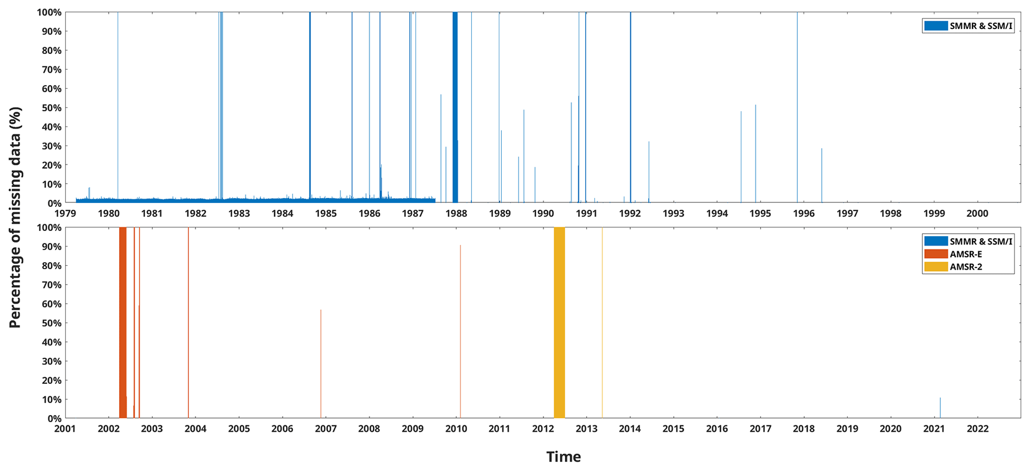
Figure A1 Daily percentage of missing data for satellite estimates. Satellite SMMR and SSM/I cover the period from 1 April 1979 to 31 March 2021. Satellite AMSR-E covers the period from 1 April 2002 to 31 March 2011. Satellite AMSR-2 covers the period from 1 April 2012 to 31 December 2021.

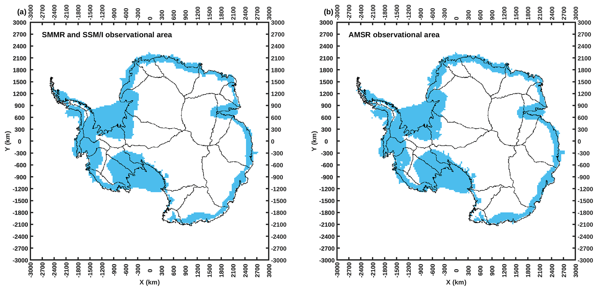
Figure A2 (a) Mask of the satellite SMMR and SSM/I observational area. (b) Mask of the satellite AMSR (AMSR-E and AMSR-2) observational area. Both masks are bilinearly remapped to the 30 km × 30 km polar stereographic grid.

Appendix B: Temperature–melt relationship

The positive relationship between 2 m air temperature and surface melt on Antarctic ice shelves (Trusel et al., 2015) allows us to use temperature to empirically estimate Antarctic surface melt via the PDD model. To assess this positive relationship, we calculate the Spearman's rank correlation between the mean summer (DJF) ERA5 2 m air temperature and RACMO2.3p2 annual surface melt amount for the period from 1979/1980 to 2019/2020. Figure 3 indicates that most of the cells in Antarctic ice shelves and drainage basin coastal zones, apart from the Ross Ice Shelf or nearby basins (17, 18 and 19), have statistically significant (p<0.05) positive correlations. Although the interior basins 19, 20 and 21 show negative correlations without statistical significance (p≥0.05), the annual melt there is negligible compared to the ice shelves and coastal areas. Overall, the correlation map shows a result consistent with Trusel et al. (2015): Antarctic ice-shelf near-surface temperature and surface melt are positively correlated, which allows us to empirically construct a temperature index model to explore surface melt in Antarctica, especially in Antarctic ice shelves.

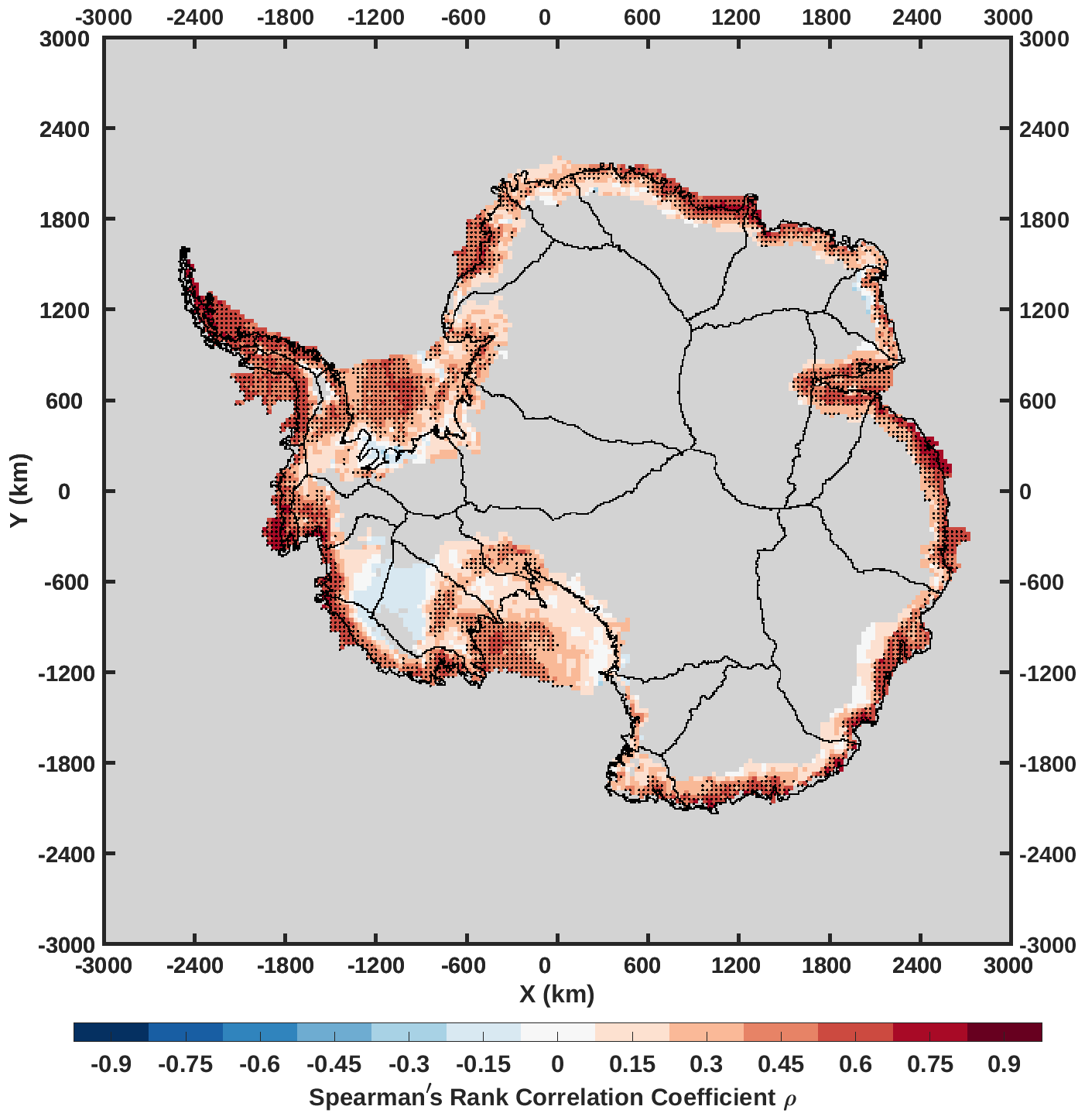
Figure B1 Correlation map between the mean DJF ERA5 2 m air temperature and RACMO2.3p2 annual surface melt amount for the period from 1979/1980 to 2019/2020. It is calculated by the Spearman's rank correlation coefficient on each cell. Black dots mark the cells where the correlations are statistically significant (p<0.05). Grey cells are either outside our research area (as shown in Fig. 1) or did not ever melt during the period.

Appendix C: Spatially uniform PDD model

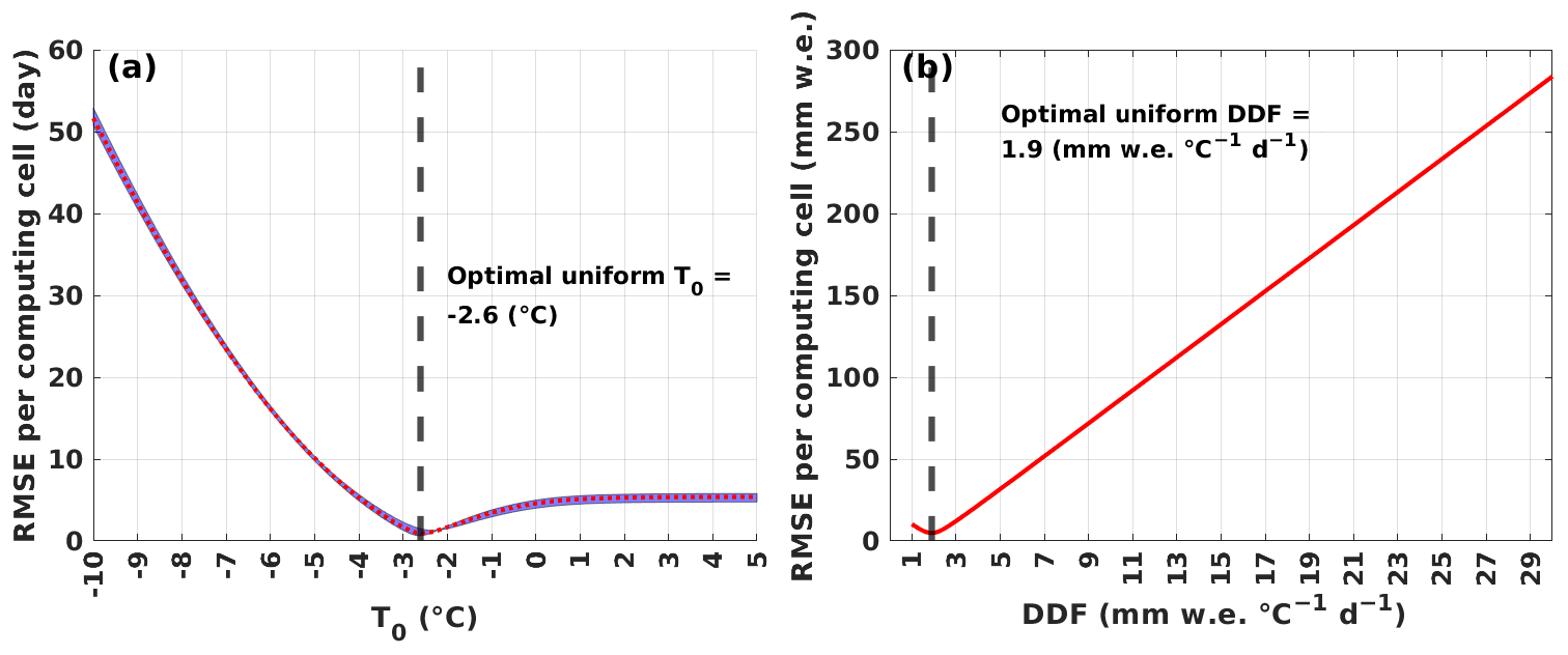
Figure C1 (a) Dotted red curve is the average of the RMSE across all satellites along each uni-PDD T₀ experiment. In each uni-PDD T₀ experiment, we calculate the RMSE between the time series of the annual sum of melt days over all computing cells between the uni-PDD model and each satellite estimate. Blue envelope covers the span of the three individual satellite results. Vertical dashed black line marks the optimal uni-PDD T₀ suggested by the minimal RMSE. (b) Red curve is the RMSE along each uni-PDD DDF experiment. In each uni-PDD DDF experiment, we calculate the RMSE between the time series of the annual sum of melt amount over all computing cells between the uni-PDD model and RACMO2.3p2. Vertical dashed black line marks the optimal uni-PDD DDF suggested by the minimal RMSE.

Appendix D: PDD model evaluation

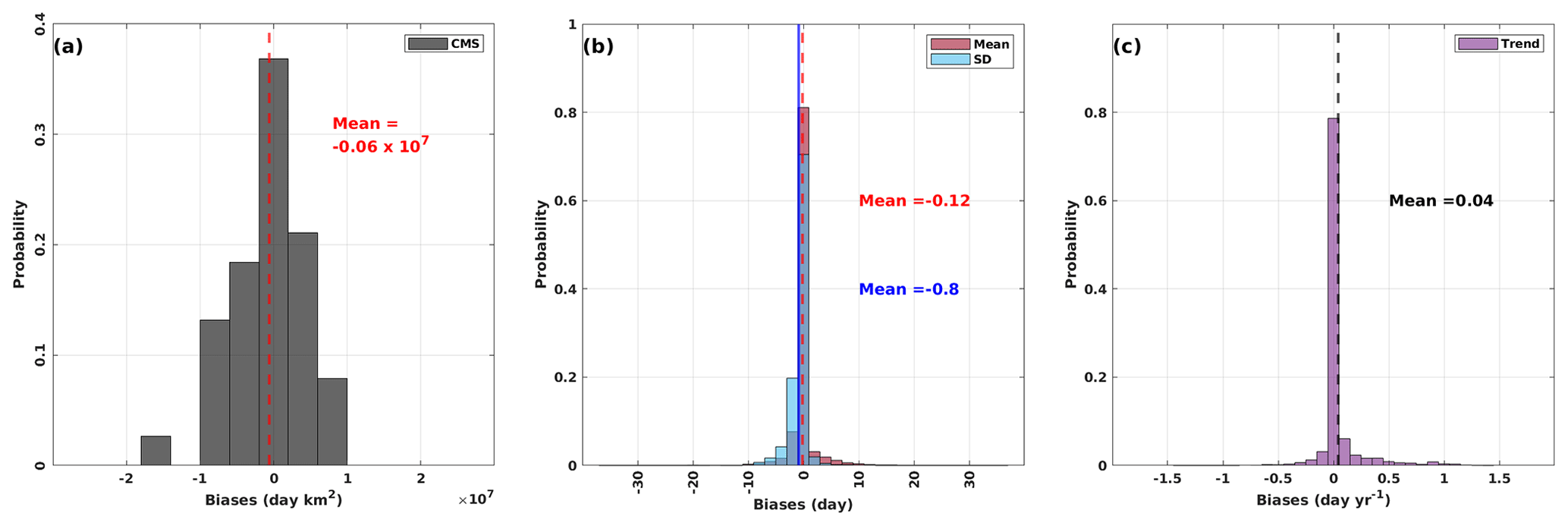
Figure D1 Panel (a): probability histogram for the biases between the dist-PDD and satellite CMS. Vertical dashed red line indicates the mean of all biases. Panels (b) and (c): probability histograms for the biases between the dist-PDD outputs and satellite estimates of mean, SD and trend. Vertical dashed red line indicates the mean of all biases between means. Vertical blue line indicates the mean of all biases between SDs. Vertical dashed black line indicates the mean of all biases between trends. Note that for all panels the satellite estimates from 2002/2003 to 2010/2011 are the average the SMMR and SSM/I sensors and the AMSR-E sensor. The satellite estimates from 2012/2013 to 2020/2021 are the average the SMMR and SSM/I sensors and the AMSR-2 sensor.

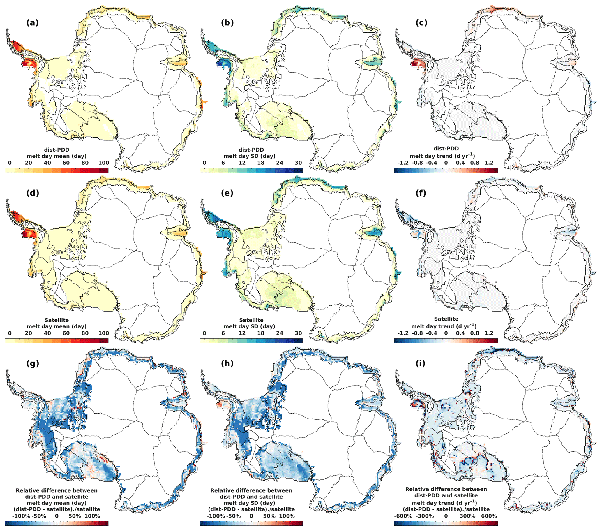
Figure D2 Panels (a) to (f): mean, SD and trend of dist-PDD/satellite melt days for the period 1979/1980 to 2020/2021 respectively. Panels (g) to (i): relative difference between dist-PDD and satellite melt day mean, SD and trend for the period 1979/1980 to 2020/2021 respectively. Note that for all panels the satellite estimates from 2002/2003 to 2010/2011 are the average the SMMR and SSM/I sensors and the AMSR-E sensor. The satellite estimates from 2012/2013 to 2020/2021 are the average the SMMR and SSM/I sensors and the AMSR-2 sensor. For all panels, the periods 1986/1987, 1987/1988, 1988/1989 and 1991/1992 are omitted.

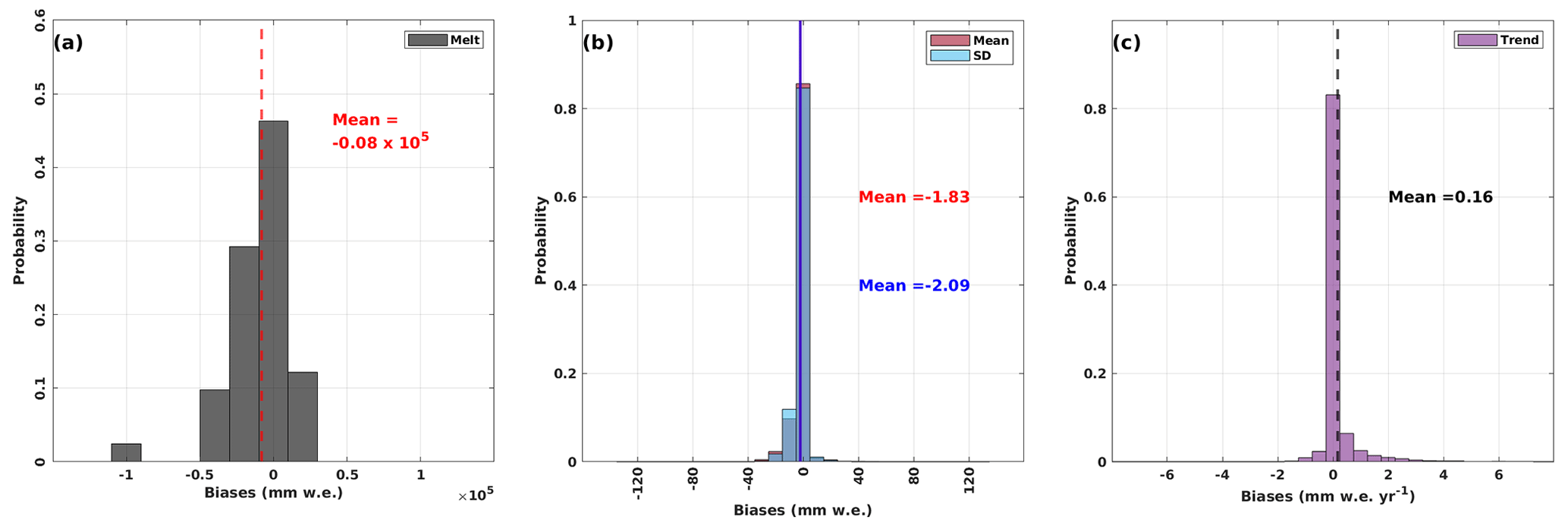
Figure D3 Panel (a): probability histogram for the biases between the dist-PDD and RACMO2.3p2 melt amounts. Vertical dashed red line indicates the mean of all biases. Panels (b) and (c): probability histograms for the biases between the dist-PDD outputs and RACMO2.3p2 simulations on mean, SD and trend. Vertical dashed red line indicates the mean of all biases between means. Vertical blue line indicates the mean of all biases between SDs. Vertical dashed black line indicates the mean of all biases between trends.

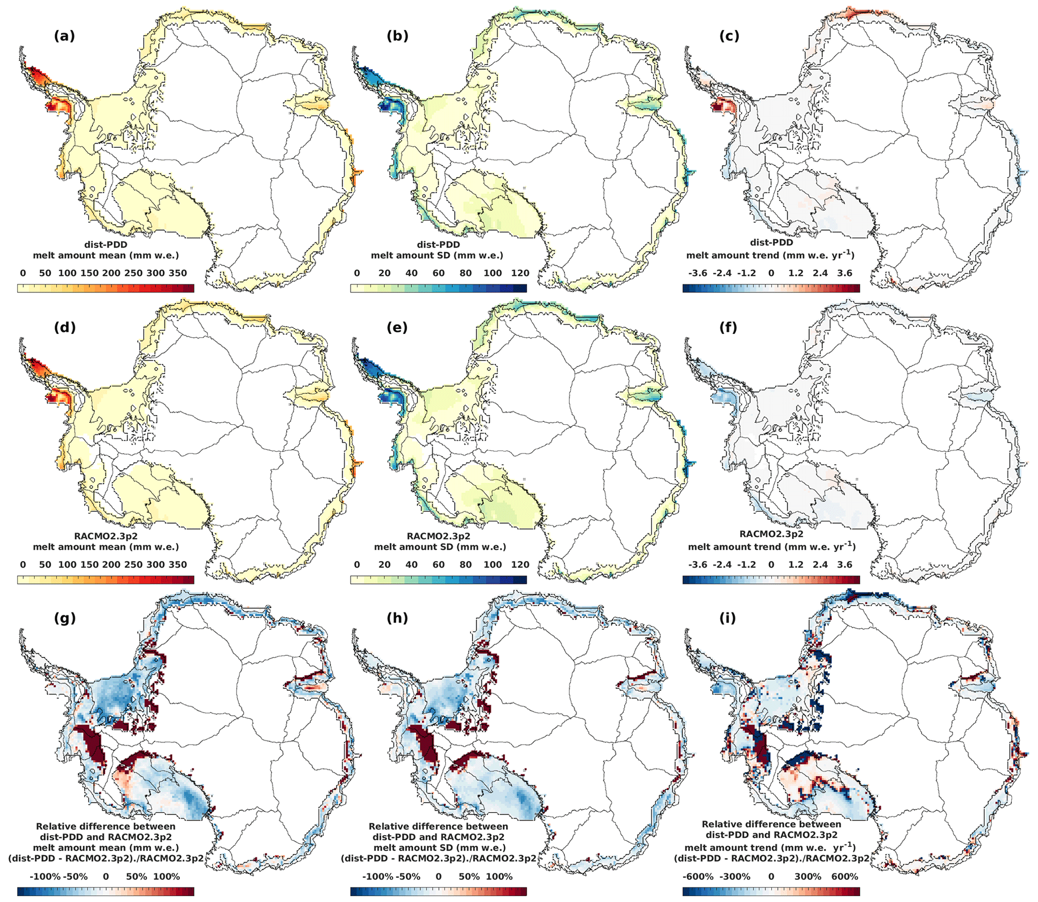
Figure D4 Panels (a) to (f): mean, SD and trend of dist-PDD/RACMO2.3p2 melt amounts for the period 1979/1980 to 2019/2020 respectively. Panels (g) to (i): relative difference between dist-PDD and RACMO2.3p2 melt amount mean, SD and trend for the period 1979/1980 to 2019/2020 respectively.

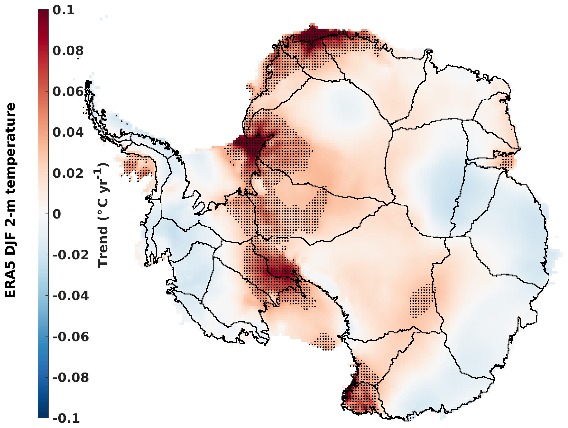
Figure D5 Trend of the mean DJF ERA5 2 m air temperature on each computing cell during the period 1979/1980–2019/2020. Black dots mark the trends that are statistically significant (p<0.05).

Appendix E: 1982/1983 event

Figure E1d and e suggest that there is a positive surface melt anomaly in the ice shelves around Amundsen Sea, Ross Ice Shelf, Amery Ice Shelf and ice shelves in Dronning Maud Land during the period 1982/1983. However, our dist-PDD model does not capture this event (Fig. E1a and b). Our dist-PDD model shows significant negative bias in both surface melt days and amounts compared to satellite estimates and RACMO2.3p2 simulations for this 1982/1983 event (Fig. E1g and h).

Both ERA5 and RACMO2.3p2 exhibit similar spatial patterns for the 1982/1983 DJF 2 m air temperature anomaly (Fig. E1c and f). Although RACMO2.3p2 is forced by ERA5 2 m air temperature, its 2 m air temperature is consistently warmer than that of ERA5 during the 1982/1983 DJF period. This is particularly noticeable in the computing cells over the ice shelves around the Amundsen Sea, Ross Ice Shelf, Amery Ice Shelf and Dronning Maud Land, where we show that significant negative biases for dist-PDD surface melt days and amounts compared to satellite and RACMO2.3p2. These cells also align with the cells where negative ERA5 2 m air temperature biases towards RACMO2.3p2 are found.

We then assess the goodness-of-fit of the dist-PDD model after removing the 1982/1983 period for dist-PDD, satellite and RACMO2.3p2. The exclusion of the 1982/1983 period significantly improves the accuracy of the dist-PDD model in comparison to satellite and RACMO2.3p2 (Fig. E2). Although there is a slight negative bias of dist-PDD (excluding 1982/1983) CMS compared to satellite data (excluding 1982/1983) in the first decade, the two CMS curves converge after approximately the first decade and almost overlap for the rest of the time period (Fig. E2a). Similarly, the cumulative melt curves for dist-PDD (excluding 1982/1983) and RACMO2.3p2 (excluding 1982/1983) show a slight divergence in the first decade but remain parallel for the rest of the time period (Fig. E2b). By the end of the integration period, the relative difference between dist-PDD and satellite CMS decreased from −3.06 % to −0.73 % (Fig. E2a), while the relative difference between dist-PDD and RACMO2.3p2 melt amounts decreased from −9.81 % to −7.52 % (Fig. E2b). These improvements are consistent across correlations and OLS linear regression analyses, as shown in Table E1, indicating the enhanced performance of the dist-PDD model in estimating both surface melt days and amounts compared to satellite and RACMO2.3p2 after excluding the 1982/1983 period.

On the basis of this additional experimentation, we are able to confidently conclude that our model is accurate for the vast majority of the time series and that any previously apparent bias was almost entirely due to the anomalous conditions of a single year.

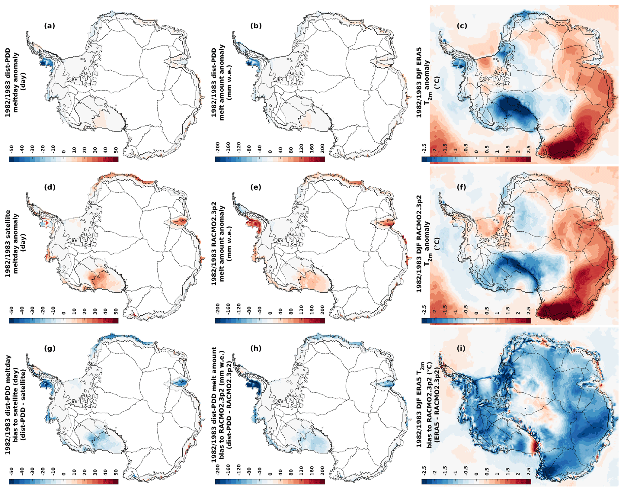
Figure E1 Panels (a) and (d): 1982/1983 dist-PDD/satellite melt day anomaly to the dist-PDD/satellite mean melt day over the period 1979/1980–2020/2021 (with 1982/1983, 1986/1987, 1987/1988, 1988/1989 and 1991/1992 omitted). Panel (g): absolute differences between 1982/1983 dist-PDD and satellite melt day. Panels (b) and (e): 1982/1983 dist-PDD/RACMO2.3p2 melt amount anomaly to the dist-PDD/RACMO2.3p2 mean melt amount over the period 1979/1980–2019/2020 (with 1982/1983 omitted). Panel (h): absolute differences between 1982/1983 dist-PDD and RACMO2.3p2 melt amount. Panels (c) and (f): 1982/1983 DJF ERA5/RACMO2.3p2 2 m air temperature anomaly to the DJF ERA5/RACMO2.3p2 mean 2 m air temperature over the period 1979/1980–2019/2020 (with 1982/1983 omitted). Panel (i): absolute differences between 1982/1983 DJF EAR5 and RACMO2.3p2 2 m air temperature. Note that for all panels the satellite estimates from 2002/2003 to 2010/2011 are the average the SMMR and SSM/I sensors and the AMSR-E sensor. The satellite estimates from 2012/2013 to 2020/2021 are the average the SMMR and SSM/I sensors and the AMSR-2 sensor.

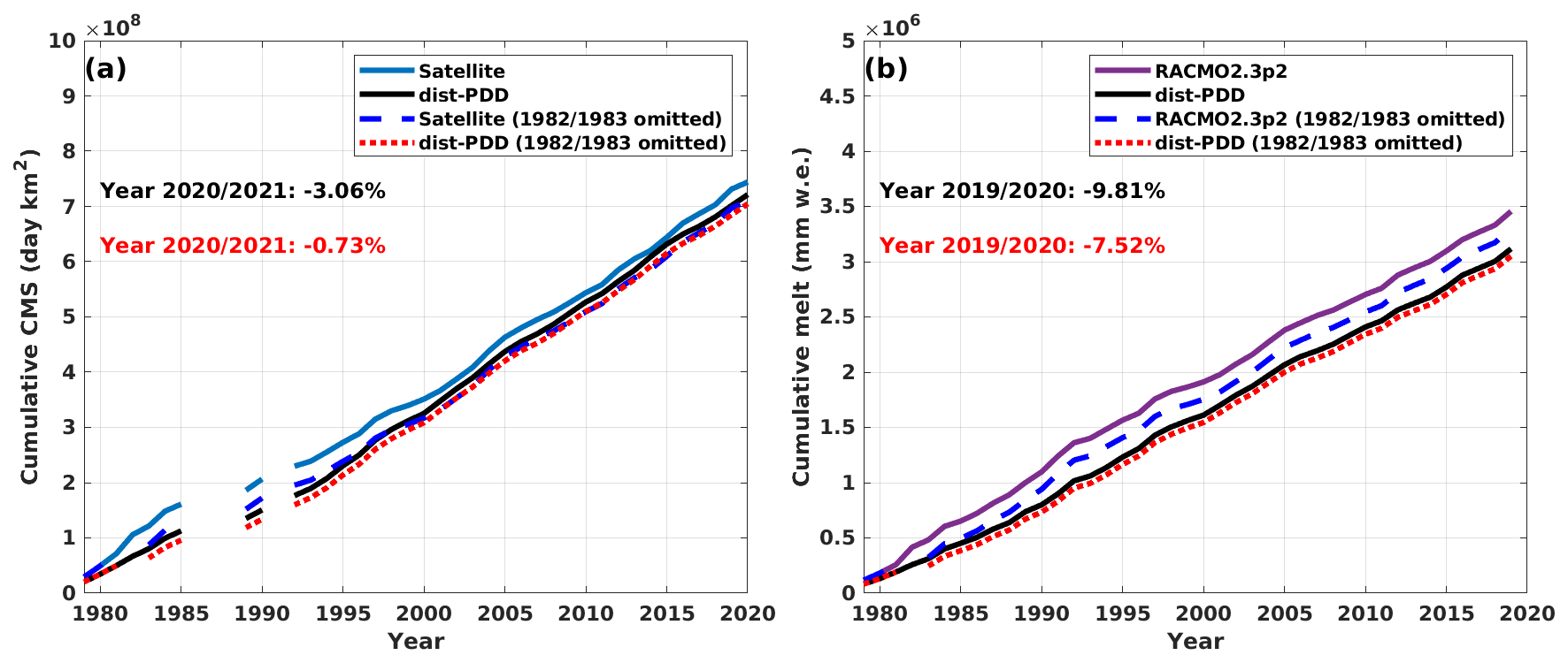
Figure E2 (a) CMS for satellite estimates and dist-PDD/dist-PDD (1982/1983 omitted) outputs from 1979/1980 to 2020/2021 (with 1986/1987 to 1988/1989 and 1991/1992 omitted. (b) Cumulative annual melt amount for RACMO2.3p2 simulations and dist-PDD/dist-PDD (1982/1983 omitted) outputs from 1979/1980 to 2019/2020.

Table E1 The Spearman's ρ and P value for dist-PDD/dist-PDD (1982/1983 omitted) CMS/melt amounts with the satellite CMS/RACMO2.3p2 melt amounts. Slope, R², RMSE and P value for the ordinary least squares (OLS) fit between dist-PDD/dist-PDD (1982/1983 omitted) CMS/melt amounts and satellite CMS/RACMO2.3p2 melt amounts. Note that the satellite estimates from 2002/2003 to 2010/2011 are the average the SMMR and SSM/I sensors and the AMSR-E sensor. The satellite estimates from 2012/2013 to 2020/2021 are the average the SMMR and SSM/I sensors and the AMSR-2 sensor. All the dist-PDD with satellite statistics are calculated over the period from 1979/1980 to 2020/2021 (with 1986/1987 to 1988/1989 and 1991/1992 omitted). All the dist-PDD with RACMO2.3p2 statistics are calculated over the period from 1979/1980 to 2019/2020.

^* 1982/1983 is omitted.

Appendix F: 3-fold CV T₀ Member 1

Figure F1 Panels (a) and (b) are same as Fig. 7m and s. (c) Time series of the CMS for satellite estimates, CONTROL and Member 1 during the testing fold period.