Multi-decadal analysis of past winter temperature, precipitation and snow cover data in the European Alps from reanalyses, climate models and observational datasets

Assessing past distributions, variability and trends in the mountain snow cover and its first-order drivers, temperature and precipitation, is key for a wide range of studies and applications. In this study, we compare the results of various modeling systems (global and regional reanalyses ERA5, ERA5-Land, ERA5-Crocus, CERRA-Land, UERRA MESCAN-SURFEX and MTMSI and regional climate model simulations CNRM-ALADIN and CNRM-AROME driven by the global reanalysis ERA-Interim) against observational references (in situ, gridded observational datasets and satellite observations) across the European Alps from 1950 to 2020. The comparisons are performed in terms of monthly and seasonal snow cover variables (snow depth and snow cover duration) and their main atmospherical drivers (near-surface temperature and precipitation). We assess multi-annual averages of regional and subregional mean values, their interannual variations, and trends over various timescales, mainly for the winter period (from November through April).

ERA5, ERA5-Crocus, MESCAN-SURFEX, CERRA-Land and MTMSI offer a satisfying description of the monthly snow evolution. However, a spatial comparison against satellite observation indicates that all datasets overestimate the snow cover duration, especially the melt-out date. CNRM-AROME and CNRM-ALADIN simulations and ERA5-Land exhibit an overestimation of the snow accumulation during winter, increasing with elevations.

The analysis of the interannual variability and trends indicates that modeling snow cover dynamics remains complex across multiple scales and that none of the models evaluated here fully succeed to reproduce this compared to observational reference datasets. Indeed, while most of the evaluated model outputs perform well at representing the interannual to multi-decadal winter temperature and precipitation variability, they often fail to address the variability in the snow depth and snow cover duration. We discuss several artifacts potentially responsible for incorrect long-term climate trends in several reanalysis products (ERA5 and MESCAN-SURFEX), which we attribute primarily to the heterogeneities of the observation datasets assimilated.

Nevertheless, many of the considered datasets in this study exhibit past trends in line with the current state of knowledge. Based on these datasets, over the last 50 years (1968–2017) at a regional scale, the European Alps have experienced a winter warming of 0.3 to 0.4 ^∘C per decade, stronger at lower elevations, and a small reduction in winter precipitation, homogeneous with elevation. The decline in the winter snow depth and snow cover duration ranges from −7 % to −15 % per decade and from −5 to −7 d per decade, respectively, both showing a larger decrease at low and intermediate elevations.

Overall, we show that no modeling strategy outperforms all others within our sample and that upstream choices (horizontal resolution, heterogeneity of the observations used for data assimilation in reanalyses, coupling between surface and atmosphere, level of complexity, configuration of the snow scheme, etc.) have great consequences on the quality of the datasets and their potential use. Despite their limitations, in many cases they can be used to characterize the main features of the mountain snow cover for a range of applications.

1 Introduction

Emissions of greenhouse gases by industrial societies since the 1850s have led to an increase in the global mean surface temperature of 1.07 ^∘C (0.8–1.3 ^∘C) and 1.59 ^∘C (1.34–1.83 ^∘C) over land (IPCC, 2021), inducing a series of modifications in the components of the Earth system. In mountainous areas, composed of a large number of systems and environments sensitive to climate change, the temperature rise has already led to major impacts (Hock et al., 2019). Observations from the past decades generally show a decrease in glacier mass, a temperature rise of the permafrost and a general decline in the snow cover duration by 5 d per decade on average at low elevations (Hock et al., 2019). These changes already impact water resources and agriculture in snow-dominated and glacier-fed river basins, as well as alter the magnitude and location of natural hazards in mountainous regions such as snow avalanches, floods and landslides (Hock et al., 2019). While many physical changes in mountain regions are already well understood in general terms, some physical processes remain imperfectly characterized such as the elevation-dependent climate changes (Pepin et al., 2015, 2022), as well as numerous impacts on a large variety of related domains, such as water resources, ecosystems and natural hazards.

Reliable observational data on essential climate variables (e.g., near-surface temperature, precipitation, snow cover area, snow water storage) are critically needed to further investigate past changes, improve process understanding, and characterize the present state of the different systems and environments under a changing climate. Yet due to multiple constraints on the installation and maintenance of a dense observational network related to the accessibility and the extreme climate conditions, the historical and current in situ coverage is sparse over mountainous regions, specifically at high elevations, even in the European Alps, one of the most extensively studied mountain ranges in the world. Multiple approaches have been developed to complement the information from sparse in situ observation networks and to gather information about the past state of the climate system in mountain regions.

Remote sensing data have the advantage of almost exhaustive spatial coverage at a high resolution (down to a few tens of meters of horizontal resolution). However, only a limited number of climate variables can be derived from them, with a short and generally partial temporal coverage that does not allow the reconstruction of past changes over the last century. MODIS (Justice et al., 1998), for example, provides records from February 2000 onwards, a time period less than the conventional 30 years required to define a climatology, let alone a climate trend. Additionally, the quality of remote sensing data is weakest in mountainous regions due to the complex topography compared to flatlands (Largeron et al., 2020).

Reanalyses are generated using a numerical weather prediction (NWP) model simulating the state of atmospheric and surface variables, using observational constraints through data assimilation. The aim of reanalyses is to provide information about the state of the atmosphere and its interfaces consistent with the observed chronology of meteorological events. Over the last decade, a new series of global and regional reanalyses have been released, taking advantage of the rise in model performance and assimilation procedures, providing high-resolution climate information. Among them, ERA5 (Hersbach et al., 2020) and ERA5-Land (Muñoz-Sabater et al., 2021) are global reanalyses recently produced by the ECMWF (European Centre for Medium-Range Weather Forecasts) and are already extensively used in a wide range of applications. UERRA MESCAN-SURFEX and CERRA-Land are high-resolution regional reanalyses resulting from a series of European projects (EURO4M, UERRA, now implemented as part of the Copernicus Climate Change Service and named CERRA), taking advantage of their high resolution and the use of a new surface analysis system MESCAN (Soci et al., 2016) to provide a robust estimation of surface variables over Europe. These new reanalyses are promising tools but are still limited for some applications. Besides their high computational cost, they remain dependent on model limitations and an assimilation system that can lead to spurious trends due in particular to the spatiotemporal heterogeneity of assimilated observations (Thorne and Vose, 2010; Vidal et al., 2010; Vernay et al., 2022).

Regional climate simulations forced by a larger-scale reanalysis are continuous long-term simulations over a limited area. They are, by design, constrained to follow the large-scale chronology of meteorological episodes and avoid some of the issues induced by the assimilation steps of regional reanalyses but inherit biases from the atmospherical model. Regional climate simulations driven by larger-scale reanalyses are mostly used as a benchmarking tool to assess the reliability of climate simulations used for climate projections. In Europe, climate simulations produced within the EURO-CORDEX framework have been used in various applications ranging from physical changes to climate change impacts (Jacob et al., 2014; Beniston et al., 2018; Terzago et al., 2017; Kotlarski et al., 2023). More recently, the EURO-CORDEX Flagship Pilot Study “Convection” has lead to the production of high-resolution regional climate simulations using climate models at kilometer scale over a domain that covers the Alpine ridge (Coppola et al., 2020; Pichelli et al., 2021). These simulations have demonstrated their potential for the study of rare events such as high precipitation events (HPEs) (Caillaud et al., 2021), as well as improved the representation of mountain variables such as temperature, precipitation and snow cover over the Alps (Lüthi et al., 2019; Monteiro et al., 2022). A recent review from Lundquist et al. (2019) suggests that high-resolution climate simulation are now able to produce a better estimate of meteorological variables over mountainous areas than gridded datasets based on in situ observations, limited by the scarcity of in situ observations and some of their observation limitations, e.g., snow precipitation wind-induced undercatch.

Several studies have focused on evaluating datasets and reanalyses in various contexts with the aim of outlining their adequate areas of use. Muñoz-Sabater et al. (2021) provide an extensive comparison of ERA5 and ERA5-Land against in situ observations for a set of surface variables (near-surface air temperature, soil moisture, snow depth). Their study highlights that besides a clear added value of ERA5-Land against ERA5 in the western US considering the representation of snow, their comparison over Scandinavia and the northern part of the Alps leads to more nuanced results which they attributed to the quality of ERA5 due to the variable density of the assimilated observation network (too low and/or unevenly distributed) in ERA5 in these regions. Isotta et al. (2015) and Bandhauer et al. (2022) focus on precipitation characteristics over the European Alps from numerous datasets (ERA5, MESCAN, EURO4M-APGD, E-OBS, etc.). They report on a widespread overestimation of accumulated precipitation and wet-day frequency of ERA5 and UERRA against gridded observational datasets and show that their local-scale performances depends on the density of the rain gauge network. Li et al. (2022) provide an intercomparison of snow depth from ERA5, ERA5-Land and Weather Research and Forecasting (WRF) climate simulations against remote sensing and observational datasets over the Tianshan Mountains in China and find contrasting results. There, ERA5-Land is prone to lower errors (RMSE and mean error, ME) compared to ERA5 at low and intermediate elevations but shows larger biases at high elevations. They both perform poorly regarding the annual evolution of snow, with an overestimated accumulation phase for ERA5 and an underestimation of the melting rate for ERA5-Land. Overall, the WRF climate simulation performs well at all elevations and gives the closer estimates of the annual cycle of snow cover. Orsolini et al. (2019) study the ERA5 abilities to represent snow characteristics (i.e., snow depth, snow cover and snow duration) over the Tibetan Plateau (TP) and find that ERA5 strongly overestimates the amount and duration of snow cover over the TP which they relate to the lack of assimilated observations in this region, as well as a strong overestimation of precipitation. Scherrer (2020) compares near-surface temperature interannual variability and trends for a set of reanalyses and gridded datasets (i.e., ERA5, MESCAN, E-OBS and COSMO-REA) against a gridded dataset for Switzerland and finds that they all perform well at low elevations but have increasing errors in terms of trends and internal variability at high elevations. Kaiser-Weiss et al. (2019) perform a broad evaluation over Europe of multiple reanalyses (those from the UERRA project and COSMO-REA) for wind, solar radiation, precipitation and temperature and find that the quality of the dataset for a given area is for a large part determined by the number of assimilated observations.

The above studies lead to nuanced results concerning the ability of recent reanalyses, gridded observation-based datasets and climate simulations to provide reliable long-term information relevant to characterize mountain meteorological conditions and the snow cover state. None of them outperforms other datasets in every region and analyzed aspects of the climatology (i.e., mean values, seasonal patterns, spatial patterns, interannual variability, trend), but they hold promising potential to complement in situ observation records. Multiple factors are involved and strongly depend on the study area such as the quality of atmospheric forcing driving the land surface model, the number and quality of the assimilated observations, and the inherited biases from the underlying model used (atmospherical model and land surface model). Thus, it is clear that extensive studies are needed to qualify the robustness of these emerging tools for their appropriate use in a wide range of downstream scientific applications.

The objective of the present study is to compare the performance of different datasets from different modeling strategies in the European Alps in order to better understand their different characteristics and assess how to provide the best possible estimate of the snow cover spatiotemporal variability and trends and its first-order drivers: wintertime near-surface temperature and precipitation. We investigate and evaluate mean seasonal and annual values, spatial variability and patterns, and interannual variability and trends over the last decades. We take advantage of the recent study by Matiu et al. (2021a) providing a consolidated dataset of in situ snow depth observations in the European Alps. We also exploit two gridded observational reference datasets: LAPrec (Frei and Isotta, 2019) for the precipitation (specifically covering the European Alps) and E-OBS for the near-surface temperature (Cornes et al., 2018). By doing so, we aim to provide information on the reliability of several commonly used and most recent reanalyses as well as other modeling approaches in the European Alps and provide estimates of climate trends in the variables from these datasets.

2 Data and methods

2.1 Study domain

Our study domain is the European Alps (see Fig. 1a), using the boundaries of the Alpine Convention (Piva Aureliano, 2020). We carry out analyses over the whole region or for the four subregions following the HISTALP division from Auer et al. (2007). These four subregions correspond to four climatically homogeneous areas: the western side (northwest and southwest) influenced by the Atlantic and a Eurasian continental regime on the eastern side. The north–south border distinguishes the warmer and drier Mediterranean side on the south (southwest and southeast) and the wetter northern part (northwest and northeast), blocking most of the western lows. This division into four main subregions based on temperature, precipitation, air pressure, sunshine and cloudiness was recently confirmed to be relevant by Matiu et al. (2021a) based on snow depth in situ observations.

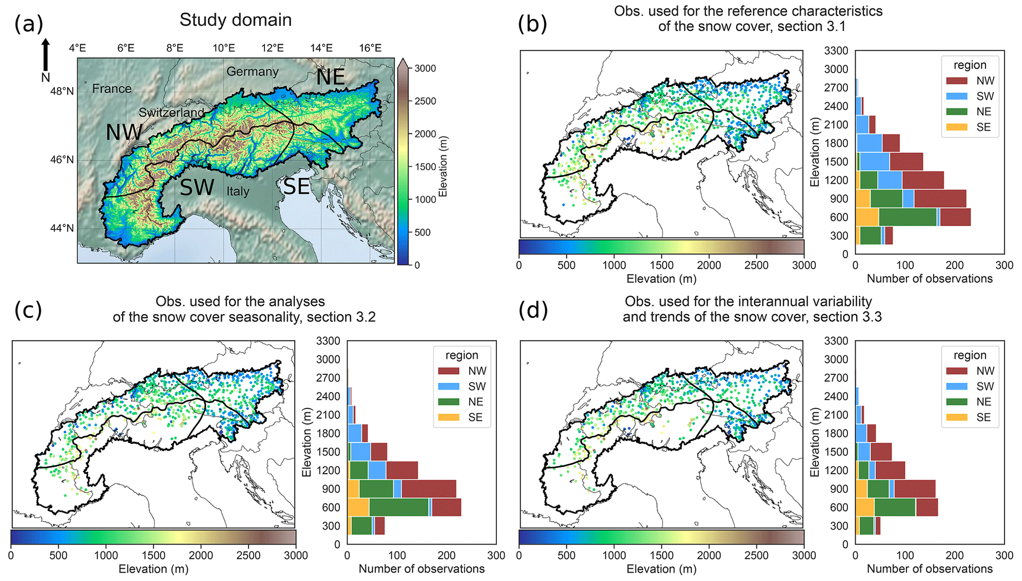
Figure 1 (a) Study domain with the DEM (digital elevation model) at 1 km resolution and contour of the Alpine Convention outline of the Alps and the four subregions. (b) Location of observations used in Sect. 3.1 with their associated number per elevation band of 300 m width for each region. (c) Same as (b) for the observations used in Sect. 3.2. (d) Same as (b) for the observations used in Sect. 3.3.

2.2 Variables of interest and indicators

Based on the availability of the variables across the datasets used in this work (model output and observations; see below), we focus on snow depth to evaluate their snow cover component.

In order to compare the evaluated datasets against remote sensing data from MODIS Terra (MOD10A1F) processed by the National Snow and Ice Data Center (NSIDC) (Hall and Riggs, 2020), three indicators are analyzed. Consecutive snow cover duration (SCD) is defined as the longest consecutive number of days in a hydrological year with a snow depth value above a given threshold value. The snow onset date (SOD) and the snow melt-out date (SMOD) characterize the beginning and the ending dates of the corresponding time period. In this study, the snow depth threshold is set at 1 cm, motivated by the minimization of error metrics, described in Sect. 2.4.3.

In the case of MODIS data, the normalized difference snow index (NDSI) value was converted to a series of binary snow cover maps (absence or presence of snow) using a threshold value NDSI >0.2. This threshold corresponds to a snow cover fraction of approximately 30 % (Salomonson and Appel, 2004). These snow cover maps were used to compute SCD, SOD and SMOD.

In addition to the state of the snow cover, we focus on near-surface temperature (2 m temperature) and precipitation amounts at the seasonal scale relevant to the winter snow cover (average and cumulated values from November to April, respectively).

2.3 Data

2.3.1 Reference datasets

In situ snow depth observation

The reference snow depth dataset is an ensemble of daily in situ observations spanning the 1971–2019 period (Matiu et al., 2021a). In this study, we used three different subsets from the overall dataset, depending on the analysis. Their locations and elevation distributions are displayed in Fig. 1. Section 3.1 focuses on the reference characteristics of the snow cover over the longest common time period from which the evaluated datasets are available. In order to have the largest spatial coverage to compute monthly to seasonal mean snow depth over large regions, we keep all station data that have at least 70 % valid daily values from November to April for the 1985–2015 period (see Fig. 1b). Section 3.2 focuses on the snow cover seasonality, using the indicators SCD, SOD and SMOD computed using continuous daily values of snow depth over the winter period, and compares it to satellite observations from MODIS (record starting in 2000). Most of the missing values happen in summer (for most of the observation stations, no snow is present during this period). In this section, we keep stations with more than 80 % valid daily values over all years of the 2000–2015 period (see Fig. 1c). Section 3.3 focuses on the interannual variability and trends. This requires the most homogeneous possible dataset along with a sufficiently long time period, so we only keep stations with more than 90 % valid daily values from November to April of the 1968–2017 period (see Fig. 1d).

MODIS remote sensing satellite observations

In order to address the spatial variability and the snow cover seasonality, we used the MODIS Terra daily normalized difference snow index (NSDI) field over the 2000–2015 period. These data from the MODIS Terra sensor have been treated by the National Snow and Ice Data Center (NSIDC) (Hall and Riggs, 2020), and they correspond to a daily gap-filled product using an algorithm described in Hall et al. (2010). In this study, MODIS NDSI data are used at their native horizontal resolution (approximately 500 m) and regridded to match different dataset resolutions (from 2.5 to 30 km) using a first-order conservative method.

Near-surface air temperature

The reference dataset of air temperature at 2 m is the E-OBS v23.1 daily mean air temperature field (Cornes et al., 2018). E-OBS is a gridded observational dataset available at 0.1^∘ (12 km) horizontal resolution over the 1950–2020 period. It is obtained by interpolating station data gathered from national meteorological services (NMSs) by the ECA&D initiative (Klein Tank et al., 2002; Klok and Klein Tank, 2009). Uncertainties (due to climatological standard error values and from the kriging procedure) are estimated using stochastic simulations to produce en ensemble of 100 realizations of each daily field, and then the spread is calculated using the 95th and 5th percentiles. In Sect. 3.3, focusing on interannual variability and trends, we used the homogenized version v19.0HOM of E-OBS. It uses a restricted number of observations, quality checked and homogenized following a procedure described in Squintu et al. (2019). E-OBS temperature values in high-mountain areas present limitations. They are known to feature a high warm bias (that can reach up to 5 ^∘C against the MeteoSwiss gridded dataset in Switzerland), resulting from the scarcity of observations used in this region at high elevations. Furthermore, the uncertainty values may be underestimated, particularly in areas with low observation density (Cornes et al., 2018).

Precipitation

The reference for precipitation is LAPrec (Frei and Isotta, 2019), a gridded dataset of monthly precipitation at 5 km horizontal resolution covering the European Alps and spanning the 1901–2019 period. It relies on a statistical approach (reduced space optimal interpolation – RSOI) combining information from a set of long-term observation stations used in HISTALP (Auer et al., 2007) and from the high-resolution gridded dataset EURO4M-APGD (Isotta et al., 2015). It is specifically appropriate for long-term studies that need a high temporal consistency while staying at a relatively large spatial scale, therefore matching the scope of this study. The user guide (Isotta et al., 2021) of this product provides an estimation of the interpolation error (in terms of mean absolute error – MAE and ME) at observation locations. The value of the MAE is 18 mm per month (all stations and months included) but is found to be larger in areas with a lower density of observations (i.e., generally at high elevations) and in summer due to the larger proportion of convective precipitation events. Additionally, systematic error measurements are not taken into account, such as the rain gauge undercatch due to wind-induced deflections of hydrometeors, known to be particularly strong at high elevations in winter (i.e., the underestimation can occasionally exceed 40 %) (Isotta et al., 2021; Kochendorfer et al., 2018, 2021).

2.3.2 Evaluated datasets

Reanalyses and climate simulations are evaluated in this study against the references described above. We however emphasize that these references are not immune to errors and serve as a common reference dataset for the purpose of this work. Figure 2 shows an overview of the evaluated datasets, their configurations, their temporal availability and their main components of interest for this study (i.e., land surface model and complexity of their snow scheme).

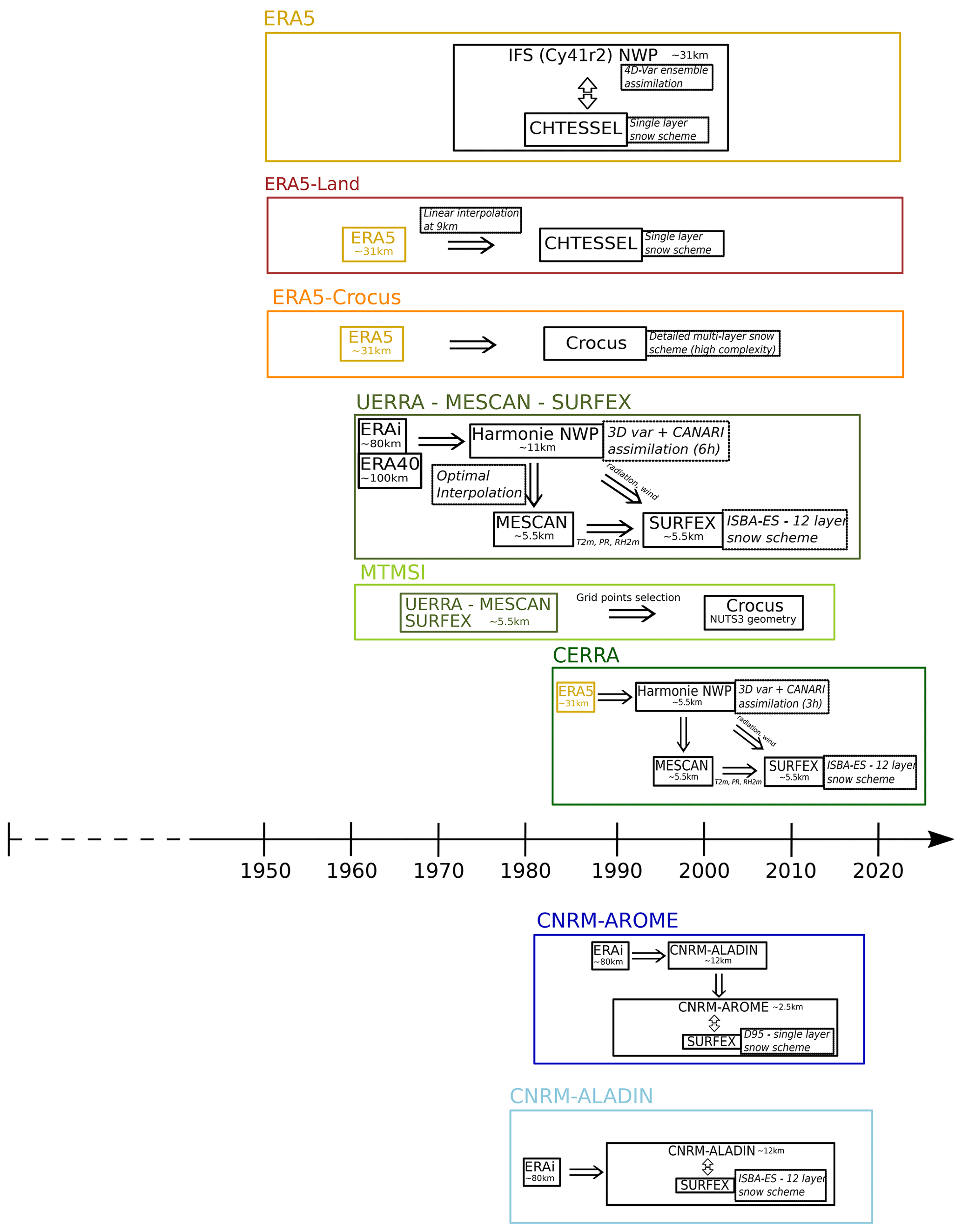
Figure 2 Schematic description of the evaluated datasets. Each dataset is represented in a colored rectangle with a width adjusted to fit its temporal coverage on the timeline. A one-way arrow indicates a driving element that is used inside another model in stand-alone mode (e.g., global driving data for regional model, atmospherical field for offline LSM run). A two-way arrow indicates a coupling between a driving element and another model. Dashed squares give specifications on their associated element.

2.3.3 Reanalyses

ERA5

ERA5 is the latest global reanalysis produced by the ECMWF using the Cy41r2 of the Integrated Forecasting System (IFS). This reanalysis provides hourly atmospherical and surface fields at a horizontal resolution of 31 km. Here we use the latest release, at the time of writing, of the reanalysis starting in 1959, while a previous version of the reanalysis was produced, starting in 1950, and is used for ERA5-Land and ERA5-Crocus (see below). A 4D-Var (variational) assimilation framework including variational bias correction is used for atmospherical fields, 2D optimal interpolation for 2 m temperature, relative humidity and snow (depth and density), and 1D optimal interpolation for soil and snow temperature (Hersbach et al., 2020). The land surface model (LSM) CHTESSEL integrates a single-explicit-layer snow model. It is an energy and mass balance model that represents an additional layer on top of the upper soil layer (Dutra et al., 2010), with its own energy budget, taking into account heat exchanges with the underlying soil and atmosphere above. It has a comparable physics to the D95 snow cover model (Douville et al., 1995) but accounts for more processes: the representation of liquid water content (as a diagnostic) and the compaction and thermal metamorphism in its snow density formulation (see Dutra et al., 2010, for more details). It is worth noting that some issues affect the ERA5 reanalysis snow depth data. Hersbach et al. (2020) note that above 1500 m in mountainous areas, snow depth can be unrealistically large due to the underestimation of melting within the snow scheme parameterization.

ERA5-Crocus

ERA5-Crocus corresponds to driving the LSM SURFEX (Masson et al., 2013) used in standalone mode along with the detailed multilayer snowpack model Crocus (Vionnet et al., 2012), using as input the meteorological fields from the ERA5 reanalysis at 31 km horizontal resolution covering the 1950–2020 period over the Northern Hemisphere. ERA5-Crocus has been used in recent analyses of Northern Hemisphere snow cover and snow cover trends, based on previous work using ERA-Interim surface atmospheric fields as input to Crocus simulations (Decharme et al., 2016; Derksen and Mudryk, 2023).

ERA5-Land

ERA5-Land is a global reanalysis produced by the ECMWF for the land component from 1950 onwards at a horizontal resolution of 9 km. It uses the ERA5 atmospherical fields downscaled at 9 km resolution using a linear interpolation with an altitudinal correction for the air temperature, humidity and pressure. The altitudinal correction is achieved using a daily environmental lapse rate derived from ERA5 vertical profiles (Dutra et al., 2020). We note that Dutra et al. (2020) only show nuanced benefits of this altitudinal correction on temperature over the western US, with even a strengthening of a cold bias against station observations when ERA5 elevation is corrected towards higher elevation, the dominant situation over high mountain ranges. These downscaled atmospherical fields are then used to force the LSM CHTESSEL (using a similar configuration as the one used in the ERA5 reanalysis), producing hourly surface fields.

UERRA: MESCAN-SURFEX

UERRA was a European project focused on the development of regional-scale atmospheric and land surface reanalyses. Multiple datasets were produced within the framework of the UERRA project. Here we used the MESCAN-SURFEX reanalysis. It is a regional reanalysis covering Europe and spanning the 1961–2019 period. It provides analyzed near-surface atmospherical and surface fields every 6 h at a horizontal resolution of 5.5 km and hourly forecast fields. It uses ERA-40 (Uppala et al., 2005) prior to 1979 and ERA-interim (Dee et al., 2011) thereafter as lateral boundary conditions (global forcing) to run the HARMONIE (HIRLAM–ALADIN Regional Mesoscale Operational NWP In Europe) NWP system at 11 km resolution (Ridal et al., 2016). An analysis is done every 6 h using a 3D-Var assimilation for the upper atmosphere and CANARI (Taillefer, 2002) for the surface. The analyzed atmospherical fields at 11 km horizontal resolution are downscaled to 5.5 km and passed to the MESCAN system (Bazile et al., 2017; Soci et al., 2016), producing an analysis of the air temperature at 2 m, the humidity at 2 m and the precipitation. These surface fields along with radiation and wind fields from the atmospherical analysis are used to drive the SURFEX LSM in standalone mode to produce surface fields at 5.5 km grid spacing. For this study, precipitation and air temperature correspond to the MESCAN analyzed fields, and snow depth values are produced by the LSM SURFEX used in standalone mode. In this configuration SURFEX uses the intermediate complexity 12-layer snow scheme ISBA-ES (Explicit Snow) (Boone and Etchevers, 2001; Decharme et al., 2016).

MTMSI

The Mountain Tourism Meteorological and Snow Indicators (MTMSI) correspond to a series of indicators generated at the pan-European scale based on a selection of grid points from the UERRA MESCAN-SURFEX meteorological reanalysis over a specific geometry (elevation bands every 100 m of elevation within each mountainous NUTS3 – Nomenclature of Territorial Units for Statistics – area) used as inputs for the detailed snowpack model Crocus from 1961 to 2015. Temperature and precipitation fields are directly derived from the MESCAN analysis, while snow depth is produced by the snowpack model Crocus. See Morin et al. (2021) for further details about this dataset.

CERRA-Land

CERRA-Land is the latest-generation regional reanalysis covering Europe from 1984 onwards, produced as part of the Copernicus Climate Change Service (Schimanke et al., 2022). It provides near-surface atmospherical and surface analyzed fields every 3 h at a horizontal resolution of 5.5 km. Its setup is almost similar to UERRA MESCAN-SURFEX. The main differences are the use of ERA5 as lateral boundary conditions, the fact that the atmospherical model (HARMONIE) runs natively at 5.5 km horizontal resolution and that an analysis takes place every 3 h using a different set of observations (higher density in some areas, different quality control).

2.3.4 Climate simulations

CNRM-ALADIN

The CNRM-ALADINv6 regional climate model (Nabat et al., 2020) uses a 12.5 km horizontal grid spacing over a large pan-European domain, 91 vertical levels and a 450 s internal time step. It is hydrostatic, which involves the parameterization of deep convection, using the PCMT (prognostic condensates microphysics and transport) scheme (Guérémy, 2011). The coupling with the LSM SURFEX includes the snow cover model ISBA-ES, using a 12-layer snowpack discretization scheme. Here, we used an evaluation run spanning the 1979–2018 period, using ERA-interim as its lateral boundaries.

CNRM-AROME

This study relies on simulations carried out with CNRM-AROME (cycle 41t1) at 2.5 km horizontal grid spacing (Caillaud et al., 2021; Monteiro et al., 2022). This version of the model was the one used operationally for NWP at Météo-France from 2015 to 2018 (Termonia et al., 2018). CNRM-AROME includes a coupling with the LSM SURFEX, using the single-layer D95 snow scheme (Douville et al., 1995). Here, we used an evaluation run spanning the 1982–2018 period that used the CNRM-ALADIN evaluation run, driven by ERA-Interim, as lateral boundary conditions (Monteiro et al., 2022).

2.4 Evaluation methods

2.4.1 Regional averaged analyses

In order to provide a common basis for the evaluation of these diverse datasets, we aggregate the temperature, precipitation and snow cover data for relatively large areas (full European Alps domain or subregions) and over elevation bands.

2.4.2 Elevation-band-based analyses

Figure 3a displays the relative frequency of the number of grid points for a digital elevation model (DEM) at 100 m horizontal resolution by elevation band and region. The DEM at 100 m is derived from the European Digital Elevation Model (EU-DEM), version 1.1 (EEA, 2016), at 25 m horizontal resolution. Figure 3b shows the difference in the relative frequency of the number of grid points for each dataset topography compared to the DEM at 100 m. It highlights that the elevation distribution over the subregions is substantially different for the various datasets investigated. Moreover, mountainous regions are known to feature a large altitudinal gradient concerning the variables of interest for this study, at least for the snow cover state and near-surface air temperature. Comparing multiple datasets at different resolutions without taking into account this unequal repartition of grid points per elevation band would inevitably induce strong systematic biases in the analysis results. Here, the analyses are carried out using averages over 300 m width elevation bands, meaning that for a given elevation band of elevation z, all stations and/or grid points with an elevation ranging between a z±150 m elevation band are combined (usually through averaging). This choice results from a trade-off between the heterogeneity within an elevation band for a given region and the inclusion of a maximum of grid points or observations within.

For most of the analyses, we chose to focus on three elevation bands, acting as a representation of three distinct environments: 600 m ± 150 m for the valleys and low-elevation hills, 1500 m ± 150 m for the intermediate elevations near the snow line, and 2400 m ± 150 m for the high-mountain conditions. Note that the results for the intermediate elevation bands (i.e., between visualized elevation bands) are generally consistent with the main patterns observed across the elevation bands analyzed and visualized.

Section 3.3 includes figures averaged over multiple elevation bands at the scale of the entire Alps. To circumvent biases induced by the large differences in the representation of the hypsometry in the different datasets (Fig. 3b), the averages over multiple elevation bands have been weighted by the relative fraction of each elevation band using the DEM at 100 m resolution as a common reference. This method ensures the same representativeness of each elevation band in the average value, regardless of the horizontal resolution of the dataset under consideration. We also exclude data below 450 m since snow has a very limited role at these elevations and above 2550 m as our datasets used are generally not designed to represent the conditions encountered at very high elevations. Overall, this leads to the exclusion of less than 12 % of the total surface area based on the DEM at 100 m resolution (see Fig. 3a).

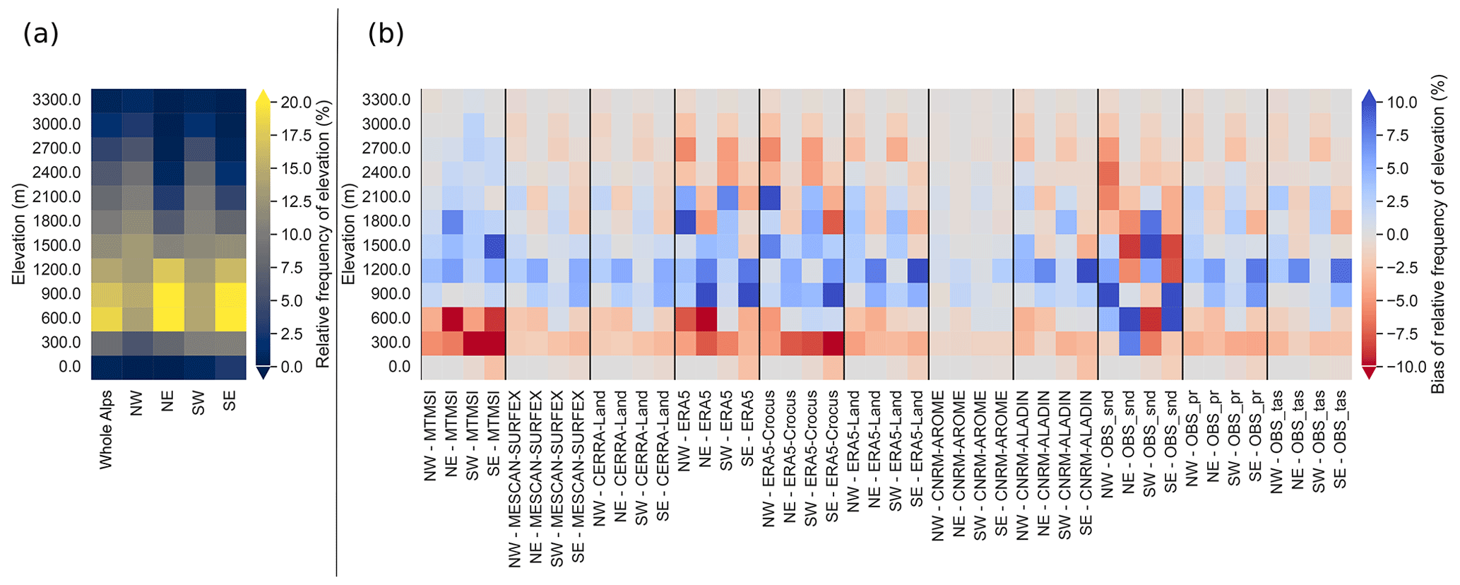
Figure 3 (a) Relative frequency of the number of grid points for 300 m width elevation bands for each region using a digital elevation model at 100 m horizontal resolution. (b) Differences in the frequency of the number of stations or grid points for 300 m width elevation bands for each region and dataset.

2.4.3 Determination of the snow depth threshold

The computation of the snow cover duration (SCD), snow onset date (SOD) and snow melt-out date (SMOD) requires as a first step converting any snow data (e.g., snow depth, snow water equivalent, NDSI) into binary data, indicating either the presence or the absence of snow. As no consensus exists for a snow depth threshold to determine the absence or presence of snow at a given location, we choose the threshold that maximizes the agreement of the snow cover detection between MODIS (with an NDSI threshold set at 0.2 to correspond to approximately 30 % of the snow-covered pixel; Salomonson and Appel, 2004) and in situ station observations (with a varying threshold of snow depth), as well as minimizing error metrics on the indicators used (SCD, SOD and SMOD). The agreement metrics used are skill scores based on the confusion matrices calculated using daily values of presence or absence of snow, considering in situ observations as the truth:

• true positive rate (TPR) corresponding to the proportion of the number of points flagged as the presence of snow in the MODIS pixel and in the corresponding in situ station

• true negative rate (TNR) corresponding to the proportion of the number of points flagged as the absence of snow in the MODIS pixel and in the corresponding in situ station

• positive predictive value (PPV) or precision being the proportion of the number of points correctly flagged as the presence of snow in the MODIS pixel

• negative predictive value (NPV) being the proportion of the number of points correctly flagged as the absence of snow in the MODIS pixel

• accuracy corresponding to the proportion of the total number of predictions that were correct (both presence and absence of snow).

Then, differences for the different thresholds between MODIS and station observations for our three indicators (SCD, SOD, MOD) are quantified using mean absolute error (MAE) and mean error (ME) values.

The stations used in Sect. 3.2 and described in Fig. 1c have been chosen because this subset covers all the elevations of interest for this study with a satisfying spatial coverage. In order to avoid altitudinal biases, stations that present elevation differences greater than 100 m with their corresponding MODIS pixel have been removed, as well as stations below 450 and above 2550 m (247 out of 941 stations have been removed). In total 694 stations over the period from 1 April 2000 to 31 December 2015 have been used, providing 3 886 400 daily observations for the calculation of skill scores and 15 seasons (2000–2001 to 2014–2015) for the SCD, SOD, SMOD MAE and biases.

Figure 4a shows that the threshold that maximizes the TNR, PPV and the accuracy while keeping a high scores of TPR and NPV is 1 cm. This threshold is lower than the 10 to 15 cm optimum found by Gascoin et al. (2015) for the Pyrenees. Possible factors that could explain the differences are a larger number of observations used in our study, covering a larger area with a larger number of low-elevation sites and a wider range of land cover. Giving a clear explanation of the differences would require further sensitivity studies that are beyond the scope of this study.

Figure 4b show the mean error metrics of the SCD, SMOD and SOD between the set of in situ observations and the corresponding MODIS pixels for the 15 seasons (from 2000–2001 to 2014–2015). On this graph, snow cover duration from the in situ observations is calculated with a varying threshold of snow depth to determine the absence or presence of snow (from 1 to 15 cm), while MODIS SCD is defined using a constant threshold of NDSI set at 20 %. Solid lines represent the mean error metrics of all locations and seasons, and shaded areas around them are the standard deviation of these error metrics between elevation classes when gathered by elevation bands of 300 m from 600 m ± 150 m to 2400 m ± 150 m.

SOD appears to be weakly sensitive to this threshold, meaning that the beginning of the continuously snow-covered season generally starts with immediately “high” values of snow depth. SMOD and SCD are more sensitive, and error metrics grow continuously with the increase in the threshold. The standard deviation is rather low for the 1 cm threshold (i.e., less than 5 d for mean error and mean absolute error), meaning that the detection performs rather similarly at all elevations. This short sensitivity study leads us to the choice of 1 cm for setting the snow depth threshold used to determine the absence or presence of snow with an uncertainty that can be large for a given station (i.e., on average 10 to 20 d) but well centered, as mean error values are close to 0. This threshold was applied to all the datasets compared with MODIS in Sect. 3.2, regardless of their horizontal resolutions, which can be considered one of the limitations of the method.

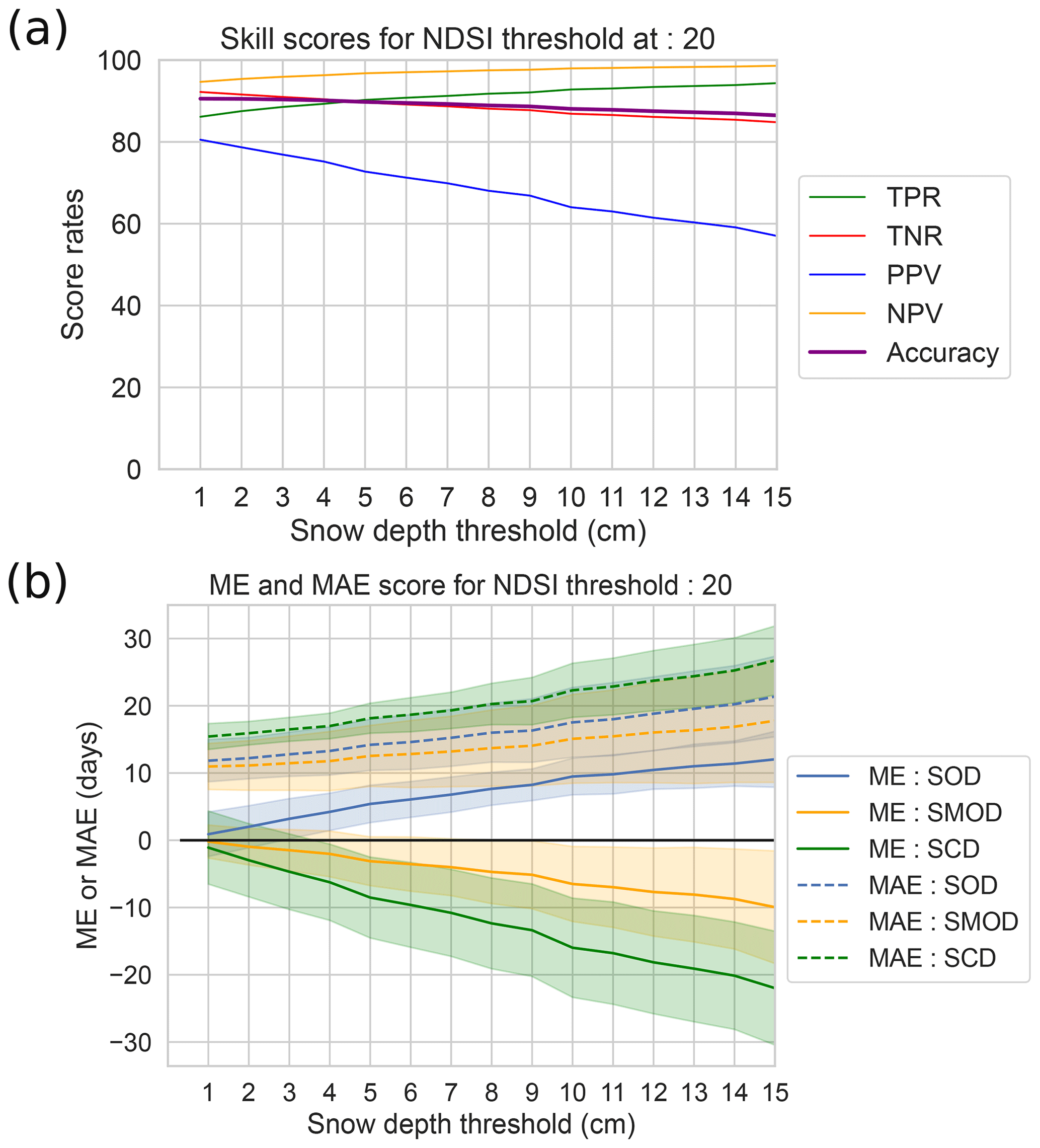
Figure 4 (a) Skill scores (true positive rate or recall – TPR, true negative rate – TNR, positive predictive value – PPV, negative predictive value – NPV, and the accuracy), calculated using the daily values of absence or presence of snow on the ground between in situ stations and MODIS pixels at station locations for various values of the threshold used to assess whether snow is present or not. See text for more details. (b) Corresponding mean errors and mean absolute errors for the SOD, SMOD and SCD indicators between the set of in situ observations and the corresponding MODIS pixels for the 15 seasons (from 2000–2001 to 2014–2015). Shaded areas represent the standard deviations between the elevation classes (from 600 m ± 150 m to 2400 m ± 150 m every 300 m).

2.4.4 Time periods, statistics and trends analyses

The reference period for the analyses in Sect. 3.1 is the longest common period available for all datasets: 1985–2015 (see Fig. 2). The method in Sect. 3.2 that focuses on snow cover seasonality mainly against MODIS data is performed over the 2000–2015 period. In these two sections, most values of the different variables are presented on average over the time period, spatially averaged for a given elevation band, over a subregion or the entire Alps.

The error metrics used are defined as follows:

• mean error $\left(\mathrm{ME}\right)=\frac{{\sum }_{i=\mathrm{1}}^N(x_i-y_i)}{N}$

• mean absolute error $\left(\mathrm{MAE}\right)=\frac{{\sum }_{i=\mathrm{1}}^N|x_i-y_i|}{N}$

• root mean square error $\left(\mathrm{RMSE}\right)=\sqrt{\frac{{\sum }_{i=\mathrm{1}}^N(x_i-y_i{)}^{\mathrm{2}}}{N}}=\sqrt{\mathrm{1}-r^{\mathrm{2}}}{\mathit{\sigma }}_y$

• correlation (Pearson linear correlation) $r_{xy}=\frac{\sum x_i{y}_i-N\stackrel{\mathrm{‾}}{x}\stackrel{\mathrm{‾}}{y}}{\sqrt{(\sum x_i^{\mathrm{2}}-N{\stackrel{\mathrm{‾}}{x}}^{\mathrm{2}})}\sqrt{(\sum y_i^{\mathrm{2}}-N{\stackrel{\mathrm{‾}}{y}}^{\mathrm{2}})}}$

with x_i and y_i being data x and y at time step i; σ_x and σ_y, respectively, the standard deviations of x and y; and N the sample size. For convenience, ME, MAE and RMSE are normalized by the mean values of the reference dataset for snow depth and precipitation.

Section 3.3 compares trends for the different variables of interest using seasonal mean winter values (November to April) for the reference and the evaluated datasets. Trends are calculated using the robust nonparametric Theil–Sen estimator, insensitive to the changing variance of the residuals (Sen, 1968), along with a Mann–Kendall test for significance assessment based on a p value threshold of 0.05. In order to verify the robustness of the method, we tested the use of the standard ordinary least squares regressions (OLSs) and the generalized least squares (GLSs) with an autoregressive component (AR(1)) to account for the effect of the interannual variability on the calculated trends, known to lead to an increase in the size of the confidence intervals (Ribes et al., 2016) and thus affect the number of trends detected as being significant. The resulting trends were of comparable values for the three methods, but the OLS method leads to the detection of more significant trends compared to the GLS with AR(1) and the Theil–Sen methods which generally share similar thresholds significance levels for our analyzed time series.

3 Results

3.1 Reference characteristics of the snow cover in the European Alps

This section presents a general evaluation of snow depth characteristics, air temperature at 2 m and precipitation for each of the datasets by comparing them against the reference datasets presented in Sect. 3.1 for the 1985–2015 period. Comparisons are described at the scale of the entire Alps, and there are not many differences in the results at the subregional scale. Figures for the four subregions are however provided in the Supplement.

3.1.1 Snow depth

Figure 5 shows an overview of the snow depth monthly time series for the different datasets over the whole European Alps. The corresponding values for the correlation, mean errors (MEs) and mean absolute errors (MAEs) compared to the reference calculated using the monthly values for the snow season (November to April) are shown in Fig. 6. In these two figures, three elevation bands are presented: 600 m (from 450 to 750 m; low elevations), 1500 m (from 1350 to 1650 m; intermediate elevations) and 2400 m (from 2250 to 2550 m; high elevations).

At all elevations in Fig. 5, all datasets present similar interannual variability, reflecting a satisfactory agreement concerning the chronology of events (see Sect. 3.3 for a more in-depth comparison of the interannual variability). This leads to high correlation scores in Fig. 6, ranging from 0.67 to 0.96, most of which are above 0.85. At low elevations in Fig. 6, CNRM-ALADIN and ERA5 present the lower correlation scores of 0.67 and 0.87, respectively, mostly explained by a shifted timing of the snow accumulation and melting phase than the reference. Their normalized mean errors are negative (−76 % for CNRM-ALADIN and −31 % for ERA5) due to a snow cover that is too thin (see Fig. 5c), a behavior that is also found for the other datasets with the exception of ERA5-Land that overestimates the amount of snow with a normalized mean error of +29 %. At intermediate and high elevations, climate simulations (CNRM-ALADIN and CNRM-AROME) and ERA5-Land systematically overestimate peak winter monthly snow depth values (see Figs. 5a, b and 6), leading to a normalized mean error between 49 % and 84 % at intermediate elevations (77 % to 184 % at high elevations). Figure 5a shows that at high elevations, snow depth values never drop below a given value for some products (0.2 and 0.3 m for CNRM-ALADIN and CNRM-AROME and 1.8 m for ERA5-Land). MESCAN-SURFEX, MTMSI, CERRA, ERA5 and ERA5-Crocus display the lowest mean errors, with normalized MAE values rarely exceeding 30 %, as well as correlation values always close to 0.9 for every elevation bands.

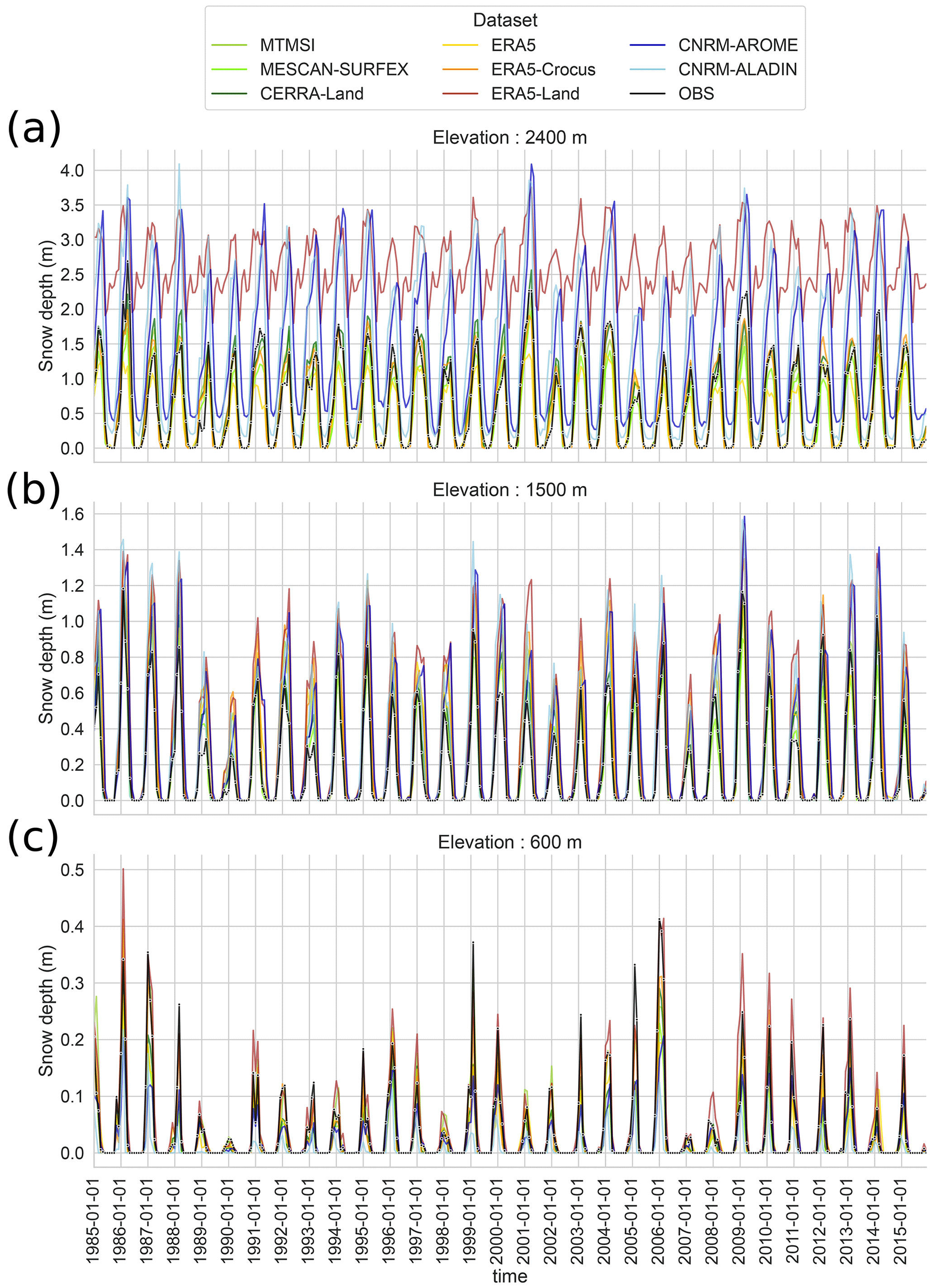
Figure 5 Time series of monthly snow depth values for each dataset for three elevation bands for the available common period, 1985–2015, over the entire European Alps domain. The reference OBS (in situ observations of snow depth) is the black line with circle markers. (a) Time series for the elevation band 2400 m ± 150 m, (b) time series for the elevation band 1500 m ± 150 m and (c) time series for the elevation band 600 m ± 150 m.

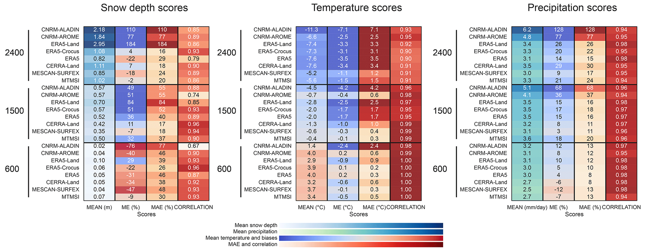
Figure 6 Mean values and scores of mean errors (MEs), mean absolute errors (MAEs) and correlations calculated using mean monthly values from November to April over the 1985–2015 period for the entire Alps and compared to the reference (in situ observations dataset for the snow depth, E-OBS for the temperature and LAPrec for the precipitation) for each dataset for three elevation bands (600 m ±150 m, 1500 m ± 150 m, 2400 m ± 150 m). Scores are presented for snow depth, temperature and precipitation, and scores of MAE and bias are normalized by the mean values of the reference (given in %) for snow depth and precipitation.

Figure 7a, b and c show, in the form of boxplots for three elevation bands, the distribution of the mean snow depth values from November to April for each dataset. Figure 7d, e and f show the corresponding annual cycle. It confirms the previous analysis and allows a more in-depth analysis of the behavior of some datasets.

At all elevations, ERA5-Land overestimates the amount of snow. In winter, snow depth values are about twice larger than the reference values at low and high elevations and around 50 % higher at intermediate elevations. It also leads to a snowpack lasting too long until melt, particularly at intermediate and high elevations, reaching its peak winter value and with a beginning of the melting period 1 month later than the reference.

CNRM-AROME also overestimates the snow depth and the duration of the snow cover at intermediate and high elevations. In this case, it is combined with a delayed accumulation phase depicted by an underestimation of the snow depth until it reaches its peak winter value. CNRM-ALADIN also exhibits an overestimation of the snow depth at intermediate and high elevations but with a reversed behavior concerning the accumulation timing. It overestimates snow accumulation at the beginning of the season with an earlier snow onset date but starts melting the snowpack 1 month earlier than the reference, similar to what was found by Monteiro et al. (2022) in the French Alps.

The amplitude and timing of the beginning, peak and end of the season are close to the reference for MESCAN-SURFEX, CERRA and MTMSI, with discrepancies concerning the snow depth within 20 % during the season. It is not surprising that only subtle differences can be seen between these three datasets, as MTMSI is a selection of MESCAN-SURFEX grid points (although with a different snow cover model), and MESCAN-SURFEX and CERRA reanalyses roughly share the same modeling systems.

The same conclusions for MESCAN-SURFEX, CERRA and MTMSI can generally be reached for ERA5 and ERA5-Crocus. They both present a satisfying average monthly evolution of the snowpack over the Alps, with differences against the reference that do not exceed 25 % and no strong deviations concerning the timing of the accumulation, peak and melting phase of the snow season. Neither of the two outperform the other in terms of mean values, ERA5 showing alternatively fewer and more differences than the reference compared to ERA5-Crocus. Nonetheless, Fig. 7d, e and f show that the use of Crocus offline driven by the atmospherical analysis of ERA5 improves slightly the monthly evolution of snow depth, leading to values closer to the reference during the accumulation and melting time periods (this is also seen for individual subregions; see Fig. A1 in Appendix A).

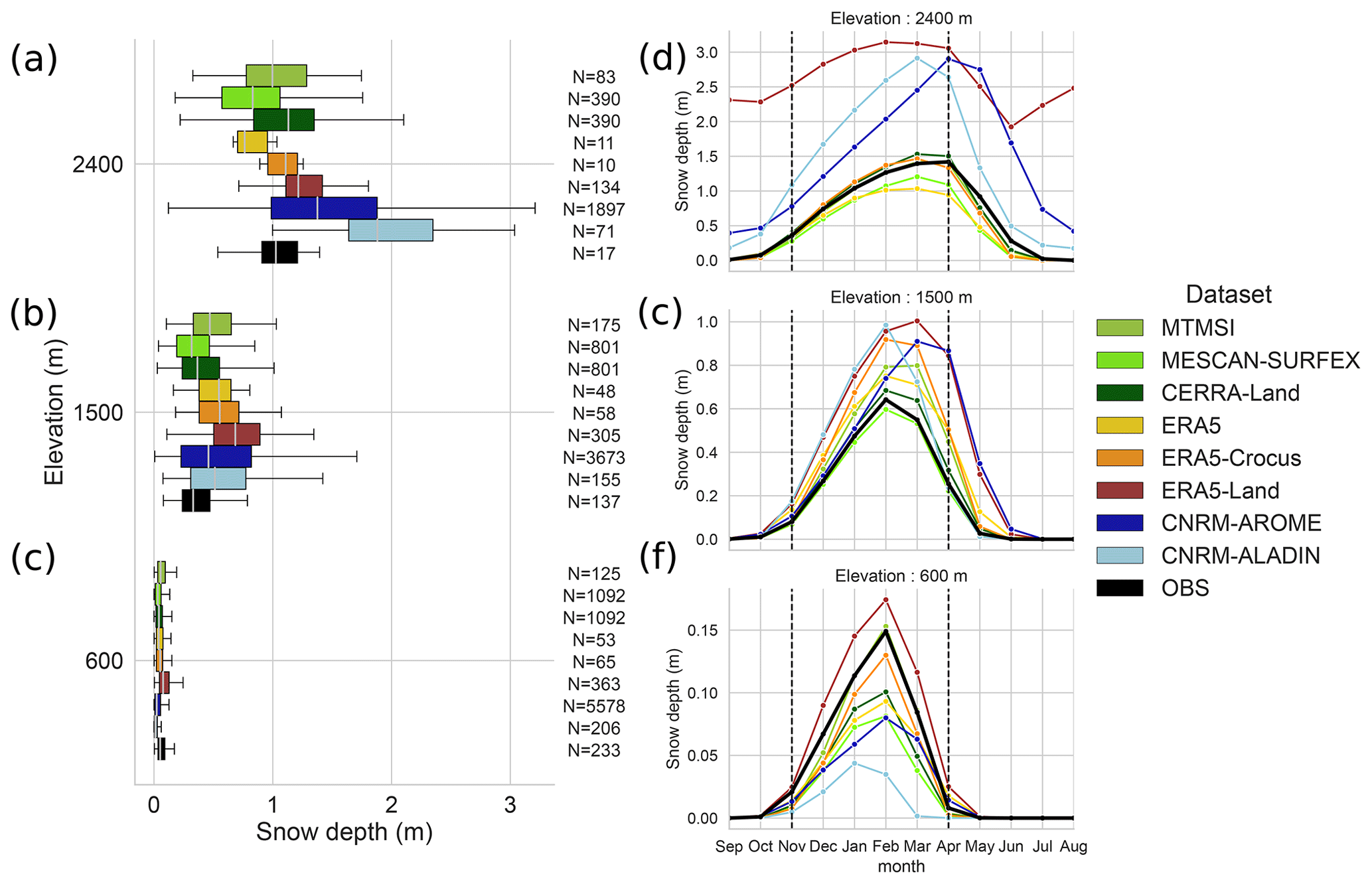
Figure 7 (a, b, c) Boxplot representing the spatial distribution of mean winter season (November to April) snow depth values over the 1985–2015 period for each dataset for three elevation bands (600 m ± 150 m, 1500 m ± 150 m, 2400 m ± 150 m) over the entire European Alps domain. (d, e, f) Annual cycle of the mean monthly snow depth values for the 1985–2015 period for each dataset for three elevation bands (600 m ± 150 m, 1500 m ± 150 m, 2400 m ± 150 m).

3.1.2 Snow driving variables: temperature and precipitation

The following subsections are dedicated to the evaluation of temperature and precipitation, following similar analyses to snow depth. Because temperature and precipitation can be considered the first-order driving variables influencing the state of the snow cover, we also aim at identifying features that could be related to the specific behavior of snow depth described before. Figure 8 shows similar results to Fig. 7 but for temperature and precipitation.

Air temperature at 2 m

At low elevations (Fig. 8c, f), most of the datasets do not exhibit significant differences with respect to the reference (i.e., outside the uncertainty range of E-OBS, ±1 ^∘C), except climate simulations (CNRM-AROME and CNRM-ALADIN), presenting similar patterns of deviations to the reference. CNRM-AROME temperature values are 1 ^∘C higher than the reference during the winter, and CNRM-ALADIN temperature values are 3 ^∘C lower at most during the spring season. These features, displayed here at the scale of the European Alps, have already been identified in the French Alps (Arnould et al., 2021; Monteiro et al., 2022).

Intermediate- and high-elevation bands in Fig. 8a, b, d and e show more contrasting results. At intermediate elevations CNRM-ALADIN and CNRM-AROME show larger discrepancies compared to E-OBS, with similar patterns overall. CNRM-AROME differences reach −1.8 ^∘C during spring and −5 ^∘C for CNRM-ALADIN in February. For ERA5-based products (ERA5, ERA5-Crocus and ERA5-Land), negative temperature differences are found and range from −2 to −3.5 ^∘C from November to February, peaking in December and January. The strongest discrepancies are found between ERA5-Land and the reference dataset. At this elevation, for MESCAN-SURFEX, MTMSI and CERRA, negative temperature differences of 1 ^∘C at most are also found for the winter months but remain within the E-OBS uncertainty range. At high elevations, there are larger differences for all datasets. Similar to low and intermediate elevations, climate simulations (CNRM-ALADIN and CNRM-AROME) exhibit negative deviations with respect to E-OBS. The strongest differences are in winter, peaking from December through February with CNRM-ALADIN temperature values being 7 ^∘C lower than E-OBS and CNRM-AROME 2.5 ^∘C lower. ERA5-based products show larger discrepancies compared to the intermediate elevation band, showing negative temperature differences around −5 ^∘C with respect to E-OBS. At this elevation, MESCAN-SURFEX, MTMSI and CERRA also display negative temperature differences for the winter months, with MESCAN-SURFEX differences from E-OBS of around −2 ^∘C and CERRA differences reaching −4 ^∘C.

For the intermediate- and high-elevation comparisons, we need to remain cognizant of the questionable reliability of E-OBS at these elevations (see Sect. 2.3.1). The negative temperature difference between all datasets and E-OBS could indeed be due to a bias of E-OBS itself. Indeed Cornes et al. (2018) show that E-OBS can exhibit higher temperature values, up to 5 ^∘C at high-elevation locations, compared to the MeteoSwiss reference temperature dataset (Frei, 2014). Nonetheless, part of these differences could also reflect a genuine negative temperature bias in the evaluated dataset as has already been shown in previous studies. Dutra et al. (2020) showed that ERA5 and ERA5-Land present a median negative temperature bias of −1 ^∘C in winter in the western US compared to a large number of in situ observations, including the Rocky Mountains. Monteiro et al. (2022) showed that over the French Alps, CNRM-AROME and CNRM-ALADIN also exhibit a negative temperature bias in winter at high elevations compared to the S2M reanalysis.

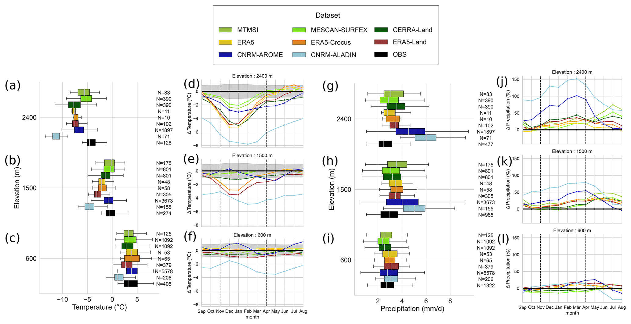
Figure 8 Panels (a), (b), (c), (g), (h) and (i) are boxplots representing the spatial distribution of mean winter (November to April) values of temperature and precipitation over the 1985–2015 period for each dataset for three elevation bands (600 m ± 150 m, 1500 m ± 150 m, 2400 m ± 150 m) for the entire European Alps domain. Panels (d), (e), (f), (j), (k) and (l) are annual cycles of the mean monthly differences in temperature and precipitation compared to the corresponding reference (E-OBS for temperature, LAPrec for precipitation) for the 1985–2015 period for each dataset for three elevation bands (600 m ± 150 m, 1500 m ± 150 m, 2400 m ± 150 m). For the temperature, the shaded areas represent the uncertainties associated with E-OBS dataset.

Precipitation

Figure 8l shows that at low elevations, rather small differences can be seen between the datasets and the reference, ranging between ±25 % of the reference precipitation amount over the winter period (November to April). The boxplot in Fig. 8i confirms that the winter distribution of the mean values at low elevations for the different datasets stays close to the reference, with slightly higher precipitation values for ERA5-derived datasets and climate simulations (CNRM-AROME and CNRM-ALADIN). MESCAN-SURFEX, CERRA and MTMSI values are close to the LAPrec distribution and mean values (Fig. 8i, l).

At intermediate and high elevations, Fig. 8g, h, j and k show that all datasets indicate a higher amount of precipitation than LAPrec, particularly during the winter season. Apart from the climate simulations CNRM-AROME and CNRM-ALADIN, differences in monthly values range between 10 % and 30 % at the beginning of winter (November) and slightly increase throughout the winter to peak in March, ranging from 25 % to 50 % at most, with the strongest discrepancies always found for ERA5-Land and CERRA. Climate simulations strongly exceed LAPrec values by 50 % and 100 % for CNRM-AROME to 80 % and 150 % for CNRM-ALADIN at intermediate and high elevations, respectively, with the largest differences at the end of winter (February to April). Figure 8g, h and i confirm that the spread in winter precipitation values and difference from the reference dataset increase with elevation.

Although winter precipitation differences are consistent among regions (not shown here; see Fig. A3 in Appendix A) and datasets, summer precipitation values display more contrasting results. Indeed, except for CNRM-AROME, most of the datasets show an overestimation of summer precipitation in the western part of the Alps at mid and high elevations, while low elevations and the eastern part of the Alps only show low and inconclusive differences. Note that the overestimation of summer precipitation for the HIRLAM model (used to produced MESCAN-SURFEX, CERRA-Land and MTMSI), ERA5 and CNRM-ALADIN has already been reported in the literature (Isotta et al., 2015; Bandhauer et al., 2022; Monteiro et al., 2022) and is attributed to their resolutions and the parameterization of deep convection.

Overall, most of the datasets simulate winter precipitation rather close to the reference, except for the climate simulations CNRM-AROME and CNRM-ALADIN that strongly overestimate it at intermediate and high elevations. Our results are in line with Bandhauer et al. (2022), who compared ERA5, E-OBS and APGD over the European Alps domain. They found an overestimation of 15 %–20 % of ERA5 winter precipitation compared to the LAPrec dataset. However, the origin of the overestimation also identified for the other datasets during the winter period may be in part due to LAPrec deficiencies. Indeed, Isotta et al. (2021) indicate that the LAPrec framework does not account for snowfall gauge undercatch. Bandhauer et al. (2022) estimated the underestimation to be close to 30 % above 1500 m in winter, and Vionnet et al. (2019) showed that a regional reanalysis assimilating unshielded rain gauges can underestimates up to 50 % of snow mass accumulation over glaciers in the French Alps. We therefore expect that, except climate simulations CNRM-AROME and CNRM-ALADIN that lead to overestimated precipitation amounts above 1500 m, the overestimation found for the other datasets could rather be due to a more realistic estimate of the winter precipitation than LAPrec. Such results are also suggested from studies in North America (Wrzesien et al., 2019). We however mention that if our results give confidence to monthly and seasonal mean winter values of precipitation for most of the datasets, they do not provides information on the temporal distribution of precipitation. For that point, it has for example been documented in Bandhauer et al. (2022) that ERA5 strongly overestimates the wet day frequency (up to a factor 2) over the Alps.

3.2 Timing of the snow cover duration against MODIS observations

In this section, we investigate further the timing of the snow season by comparing the evaluated datasets against remote sensing data from Terra/MODIS MOD10A1F (MODIS in the following) over the 2000–2015 period. The comparison is carried out using indicators that can be defined using either the snow depth or the normalized difference snow index (NDSI): the snow cover duration (SCD), the snow onset date (SOD) and the snow melt-out date (SMOD) (see Sect. 2.2 and 2.4.3 for further details). Figure 9a and b show maps and boxplots of the mean error between the evaluated datasets and MODIS. To this end, MODIS-based indicators were interpolated using a first-order conservative regridding over each dataset grid. This section does not include the MTMSI dataset because of its peculiar geometry (elevation bands over NUTS3 areas). We also exclude CNRM-ALADIN simulations because daily snow depth values are not available.

Figure 9a and b reveal positive differences across elevation bands, regions and datasets compared to MODIS, indicating a general overestimation of the snow season duration (SCD) in the evaluated datasets. Looking at the boxplot differences for the entire Alps (Fig. 9b) brings more details about the elevational distribution of differences as well as their magnitude. All datasets display differences from MODIS values, which differ with elevation, peaking at intermediate elevations with median mean error (ME) ranging from 20 to 70 d.

The amplitude of the overestimation compared to MODIS is the strongest and the most spatially extended for ERA5-Land, exceeding 100 d in some locations (Fig. 9a) with median mean error ranging from 40 to 75 d (Fig. 9b). This confirms the issues with ERA5-Land snow cover data, consistent with the general overestimation of snow depth values and the spurious snow accumulation occurring above 2000 m, shown in Sect. 3.1 and Figs. 5, 6 and 7.

ERA5 and ERA5-Crocus data show lower mean error values than ERA5-Land, with the largest differences in the western part of the Alps for ERA5. The median of the mean error values ranges from 20 to 50 d for ERA5 and 10 to 40 d for ERA5-Crocus. While ERA5-Crocus does not show substantial improvements over ERA5 in terms of snow depth (see Sect. 3.1.1), it provides results closer to the reference in terms of snow cover duration. MESCAN-SURFEX and CERRA snow cover duration data show similar patterns with either over- or underestimations compared to MODIS. Indeed, Fig. 9a shows an underestimation of the SCD of 10 to 30 d (beyond 50 d at specific locations) over the inner-Alpine ridge near the northwestern and southwestern boundary and an overestimation elsewhere, ranging from 10 to 50 d. Their distribution of mean error values are overall more centered around 0 than the other datasets. MESCAN-SURFEX shows the lowest differences overall, and we note that CERRA particularly overestimates the SCD in the western Italian Alps.

For CNRM-AROME, the map in Fig. 9a shows an elevational pattern with a slight underestimation of the snow cover duration in valleys and an overestimation elsewhere. The boxplot in Fig. 9b confirms it, revealing biases centered around 0 at low elevations and a generalized overestimation above. This is in line with its snow depth underestimation at low elevations and overestimation at intermediate and high elevations described in Sect. 3.1.

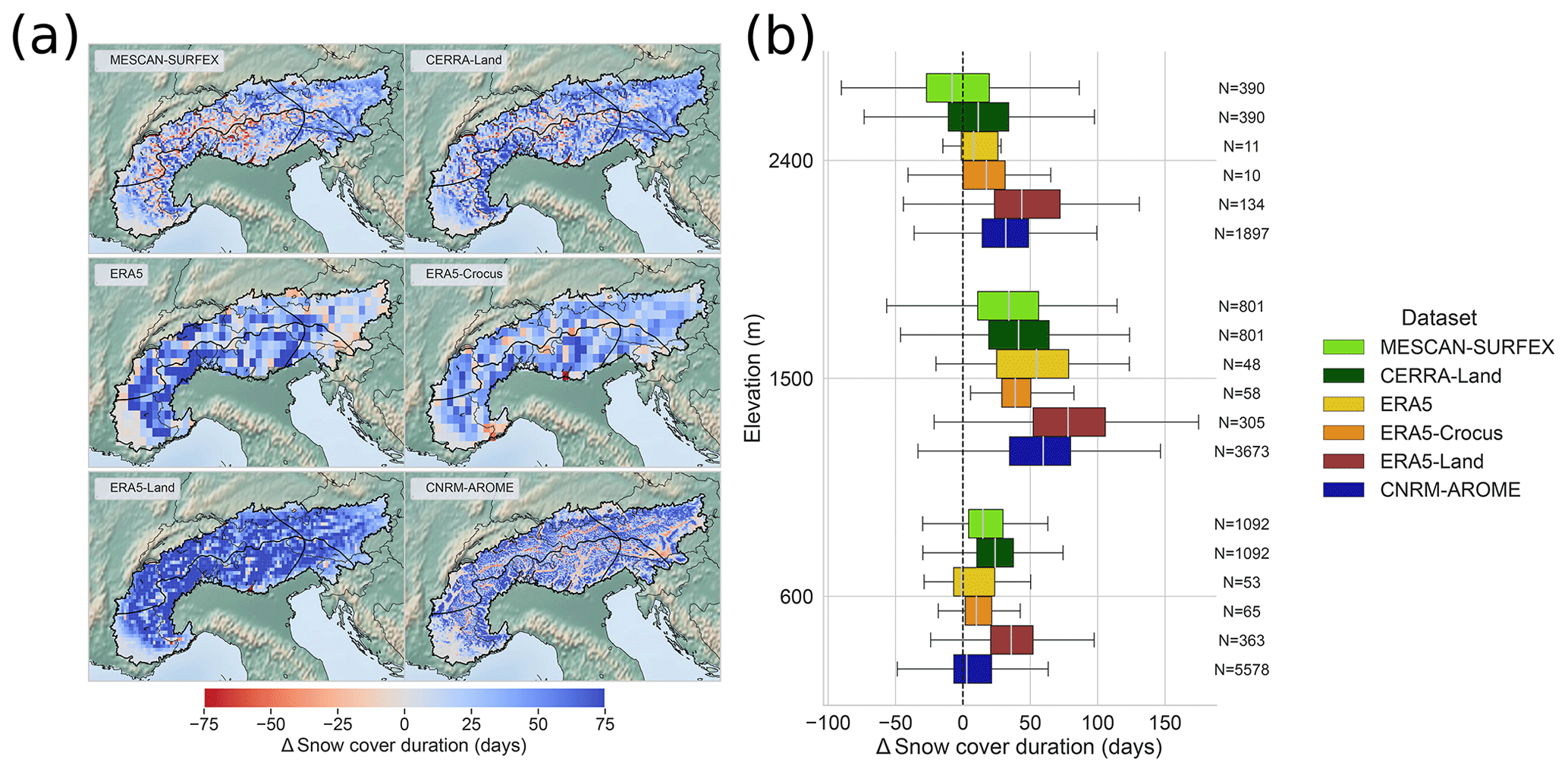
Figure 9 Snow cover duration differences between the evaluated datasets and MODIS observations in the European Alps. Note that MODIS products initially at 500 m horizontal resolution have been regridded over each dataset grid using a first-order conservative method. (a) Map of the average differences (mean error) in the snow cover duration (SCD) over 15 seasons (2000–2001 to 2014–2015) for each dataset compared to MODIS SCD. (b) Boxplot representing the spatial distribution of the average differences (mean error) of the SCD over 15 seasons (2000–2001 to 2014–2015) compared to MODIS SCD for each dataset for multiple elevation bands.

Figure 10 provides information about the timing of the snow season by displaying the mean values of the snow onset date (SOD) and snow melt-out date (SMOD) as the edges of the bar plot, while the bar plot length corresponds to the snow cover duration (SCD). The error bar represents the spatial variability (using the standard deviation) of the SOD and SMOD for each dataset and MODIS at its native resolution.

Combining the information of Figs. 9a and b and 10a, b and c shows that the snow cover duration is overestimated by all datasets, compared to MODIS, for all elevation bands. From Fig. 10a, b and c, the size of the error bars informs us about the spatial variability in the SOD and the SMOD. From it, we can conclude that it is underestimated in all datasets except for CNRM-AROME, but it may be partly related to the lack of horizontal resolution in most of the datasets.

At low elevations (Fig. 10c), MESCAN-SURFEX, CERRA and ERA5-Land provide SOD values close to MODIS, but SMOD values are too late by up to 15 d, i.e., 30 % longer SCD altogether. At this elevation ERA5-Crocus SOD and SMOD are rather close to the MODIS values, while ERA5 SOD occurs 15 d later and CNRM-AROME SOD 7 d earlier, despite a close overall SCD. We note that in situ observations also provide values towards a later beginning and longer lasting snow season compared with MODIS estimates.

At intermediate elevations (Fig. 10b), all datasets overestimate the duration of the snow season from 30 to 100 d at most, with an earlier SOD and a later SMOD compared to the MODIS dataset. ERA5-Land and ERA5 results provide the longest SCD (around 170–200 d), while MESCAN-SURFEX, CERRA, ERA5-Crocus and CNRM-AROME provide SCD values, ranging from 135 to 150 d closer to MODIS values (about 100 d). At this elevation, the range of values of in situ observations of SOD and SMOD are close to the range of values of MODIS, with an earlier mean of SOD and later mean of SMOD for the in situ observations that may be due to the oversampling of sites with a longer snow cover duration.

At high elevations (Fig. 10a), whereas all datasets indicate a SOD value earlier than MODIS (around 15 d earlier), MESCAN-SURFEX, CERRA, ERA and ERA5-Crocus SMOD values are in agreement with MODIS values. ERA5-Land and CNRM-AROME SMOD values are 15 to 30 d later than MODIS-based estimates.

This comparison with MODIS indicators adds another perspective to Sect. 3.1: despite different behaviors concerning snow depth values at the monthly or seasonal scale, all datasets overestimate the duration of the snow season at all elevations compared to MODIS-based information. This is rather due to a late snow melt-out date rather than an earlier snow onset date, with the largest discrepancies occurring at intermediate elevations. This relates to the fact that the snow melt-out date results from cumulated processes throughout the winter season, making it more difficult to estimate than other snow cover indicators.

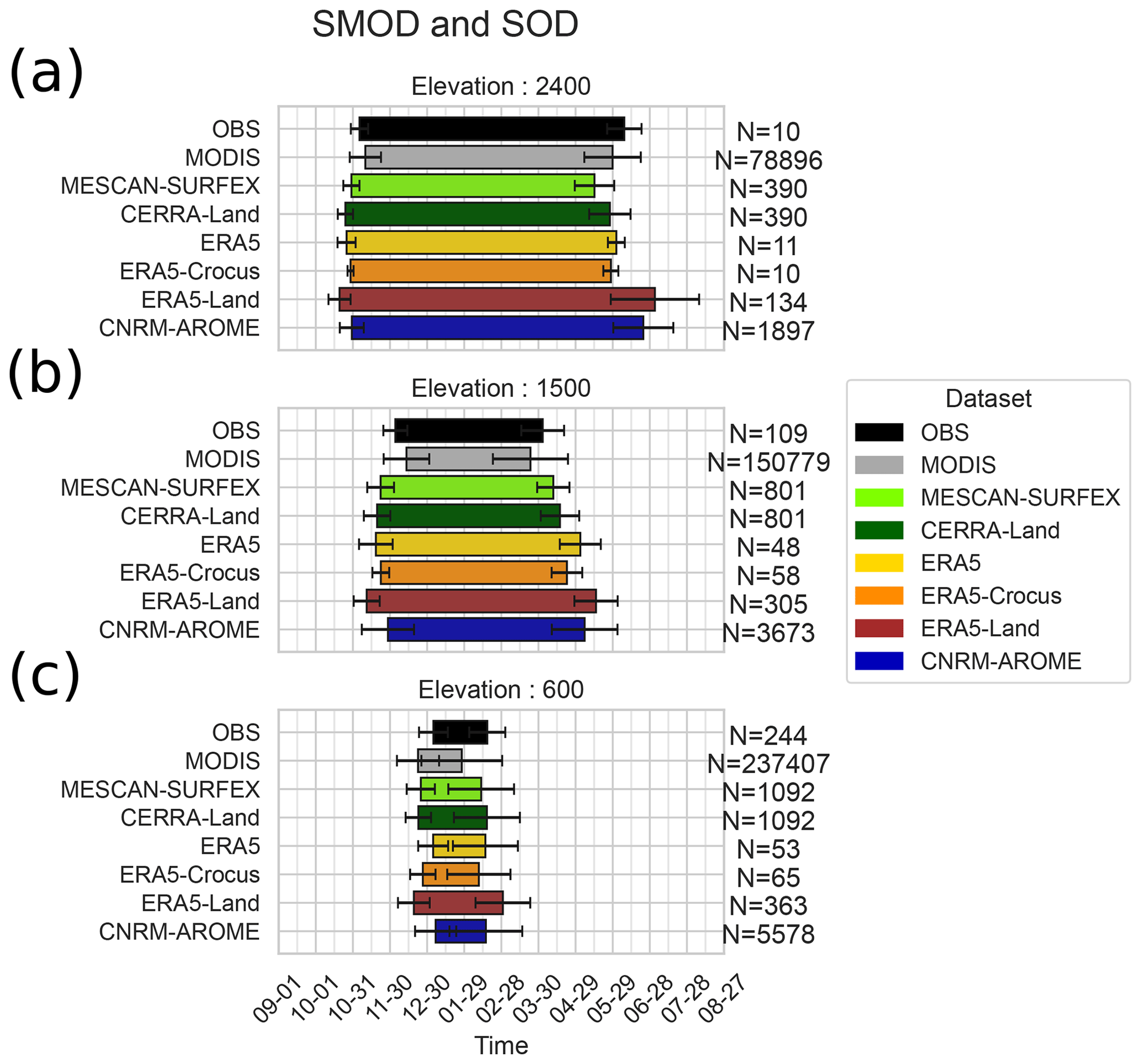
Figure 10 Bar plot whose edges represent the spatial mean over the Alps of the snow onset date (SOD) and the snow melt-out date (SMOD) for 15 seasons (2000–2001 to 2014–2015) for three elevation bands (a – 2400 m ± 150 m; b – 1500 m ± 150 m; c – 600 m ± 150 m) for each dataset at their native resolution. The error bars surrounding the edges of each bar represent the standard deviation of the spatial distribution of mean values of the SOD and the SMOD.

3.3 Interannual variability and trends

In this section we analyze and compare the time variability and past trends for the winter season (November to April) obtained using our reference and evaluated datasets over multiple time periods for most of the indicators addressed in this study: the snow depth, the snow cover duration, the air temperature at 2 m and total precipitation. For both the anomaly and the trend analyses, we use a subset of in situ snow observation stations with less than 10 % missing values during the 1968–2017 snow period (taking the daily values from November to April) (see Fig. 1d and Sect. 2.3.1 for more details). For the same reason, we use the homogenized version of E-OBS (v19.0HOM) for air temperature at 2 m.

Anomalies are computed using the 1985–2015 climatology as reference (absolute differences for snow cover duration and temperature, relative differences for precipitation and snow depth). Taylor diagrams are calculated using anomalies for the common available time period: 1985–2015 (also used in Sect. 3.1). Linear trends are estimated using the Theil–Sen nonparametric estimator along with a Mann–Kendall test for significance assessment based on a p value threshold of 0.05.

3.3.1 Representation of the interannual variability in the evaluated dataset

This subsection compares the representation of the interannual variability between the different products and the reference datasets.

Figure 11 shows the time series of winter (November to April) anomalies for temperature, precipitation, snow depth and snow cover duration. For each variable and dataset, Taylor diagrams based on winter anomaly time series for the 1985–2015 period are also displayed. In addition, Figs. B1, B2, B3 and B4 in Appendix B display the anomalies at a subregional scale.

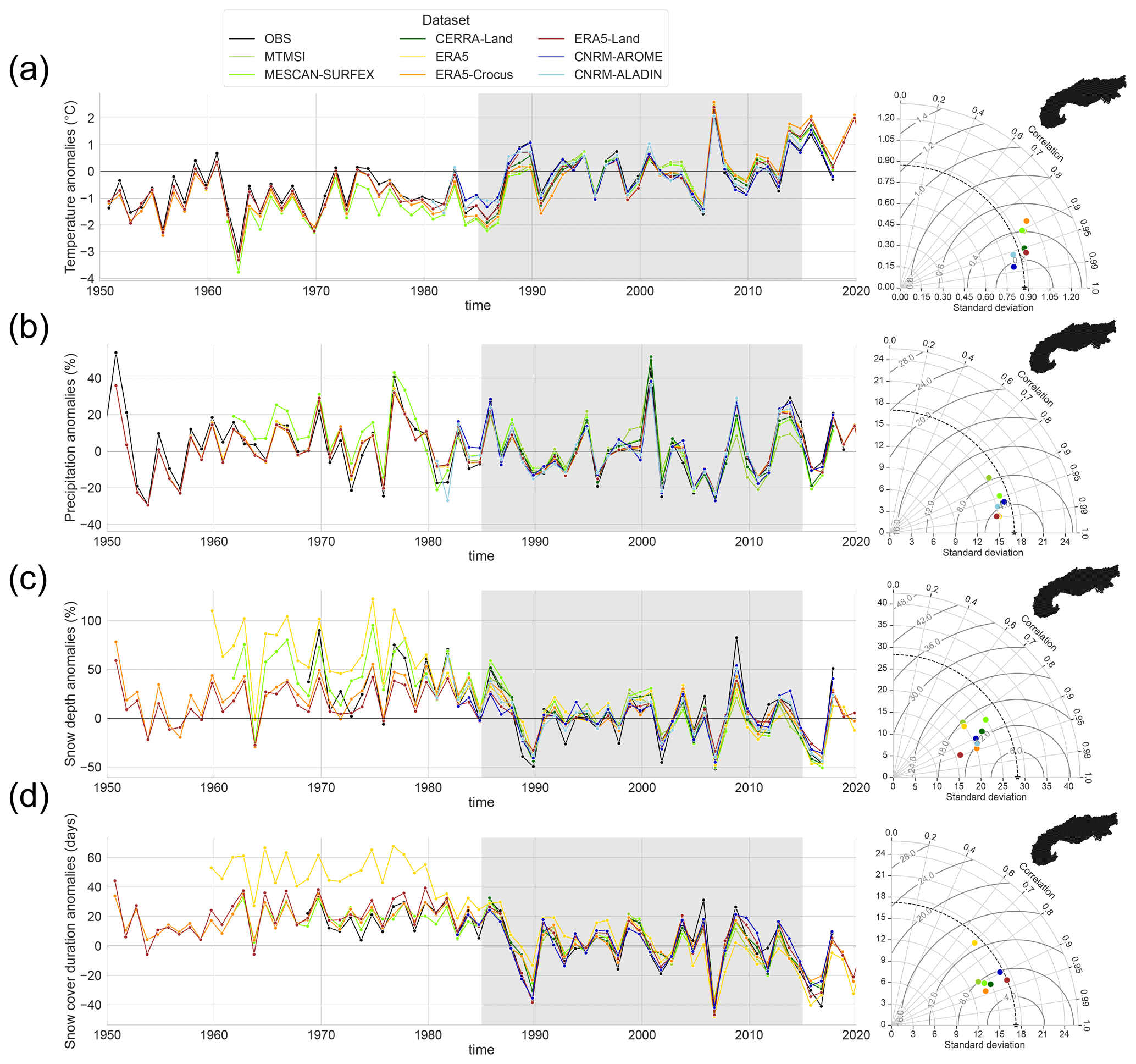
Figure 11 Anomalies of mean winter (November to April) values in the European Alps for the whole available time period for each dataset compared to the mean winter values of the 1985–2015 period (shaded area). On the right, Taylor diagrams calculated using the anomalies of winter values for the 1985–2015 period (shaded area). The reference used is described in Sect. 2.3.1. Four variables are displayed: (a) temperature, (b) precipitation, (c) snow depth and (d) snow cover duration.

Temperature anomalies in Fig. 11a show high correlation values (always above 0.8) with respect to the reference dataset, with a standard deviation of anomalies close to the standard deviation of the reference (0.8 to 1.0 ± 0.2 ^∘C, i.e., less than 20 % difference from the reference) meaning that anomalies are of comparable amplitudes between datasets. Climate simulations (CNRM-AROME and CNRM-ALADIN) and ERA5-Land show the highest scores of correlations. CNRM-AROME and CNRM-ALADIN slightly underestimate the amplitude of the anomalies, while ERA5-Land is closer to the reference in this respect or with a slight overestimation. ERA5, MESCAN-SURFEX, MTMSI and CERRA datasets show the lowest correlation values and overestimate the amplitude of anomalies. Figure B1 in Appendix B shows that the anomalies follow comparable fluctuations among subregions, indicating that most of the interannual variability occurs at a larger spatial scale, affecting the whole Alpine region similarly. In a comparison of temperature anomaly errors between multiple datasets including MESCAN-SURFEX, ERA5, E-OBS (v19.0HOM) and COSMO-REA6 (a regional reanalysis at 6 km horizontal resolution that does not assimilate near-surface temperature) against a set of homogenized in situ observations over the Swiss Alps, Scherrer (2020) came to similar conclusions: the lowest scores (higher mean errors in this case) are found in winter and at elevations above 1000 m for MESCAN-SURFEX and ERA5, whereas COSMO-REA6 does not present significant error differences between summer and winter and low and high elevations. The explanations put forward are twofold: (i) the insufficient resolution of ERA5 that does not allow us to capture the altitudinal gradient of temperature anomalies that can be strong in winter when there are interplays between synoptic flow and local topography and (ii) the assimilation of near-surface temperature for MESCAN-SURFEX that seems to be problematic in high-elevation regions. We note that in the eastern part of the Alps (regions NE and SE in Fig. B1 in Appendix B), CERRA provides better scores than MESCAN-SURFEX, and it may be the result of a more selective assimilation procedure in this region (i.e., the assimilation of fewer and/or higher-quality observations).

Precipitation anomalies (Fig. 11b) show a good agreement between datasets with all correlation values above 0.85 and a rather close, albeit slightly underestimated standard deviations of anomalies for all datasets. A graphical comparison of the time series of anomalies in Fig. B2 in Appendix B shows rather strong differences between subregions. Indeed, winter precipitation anomalies appear to be weakly correlated between subregions compared to the temperature anomalies, implying that interannual variability in winter precipitation has a strong subregional component within the European Alps.

Snow depth anomalies (Fig. 11c) show lower agreements between datasets than temperature and precipitation anomalies, with correlation values varying from 0.75 to 0.95, with an amplitude of anomalies underestimated by all the datasets compared to the in situ observation dataset. At every scale (i.e., regional to subregional), snow depth exhibits a higher variability than temperature or precipitation. The amplitudes of anomalies of mean winter snow depth span ±100 %, with peaks over ±200 % for the eastern regions in Fig. B3 in Appendix B. Comparing the amplitude and the correlation of the anomalies with the reference dataset does not allow us to identify a dataset which outperforms all others. However, we note that ERA5 between 1950 and 1980 shows significantly higher anomaly values along with a large increase in their standard deviations specifically for the western region (northwestern and southwestern), a behavior specific to ERA5. It is due to some low-elevation grid points (below 1000 m) showing a strong decrease in their mean winter snow depth values from 1980 onwards that may be in part an artifact induced by the strong increase in the number of assimilated snow depth observations after the 1980s.

Snow cover duration anomalies (Fig. 11d) also present a lower agreement among the datasets than winter temperature and precipitation with correlation values between 0.7 and 0.95. The amplitudes of anomalies are also slightly underestimated by most of the datasets as shown by the ratio of the standard deviation between the datasets and the reference within the Taylor diagram in Fig. 11d. Figure B4 in Appendix B confirms that no dataset outperforms the others in terms of correlation scores, RMSE and ratio of the standard deviation, just as for snow depth, but ERA5 systematically shows the lowest scores. Correlation scores of ERA5 barely exceed 0.7 and drop to 0.6 for the northwestern region, indicating a low agreement concerning the fluctuations in the anomalies. Additionally, ERA5 snow cover duration anomalies also show the strong shift in the mean values of anomalies from before 1980 to after that we relate to the same causes as for the snow depth.

3.3.2 Running window trend analysis

This section compares the long-term trends in the snow variables (snow depth and snow cover duration), temperature and precipitation. Trends are calculated using the mean seasonal values for the winter period (November to April) using the Theil–Sen linear regression, and significance levels are assessed using a Mann–Kendall test based on a p value threshold of 0.05. As for Sect. 3.2, CNRM-ALADIN is not included for the SCD indicators because daily fields of snow depth values are not available.

Figures 12 and 13 display the trend values for the winter values of temperature, precipitation, snow depth and snow cover duration for each dataset, calculated using different window time durations (10, 20, 30, 40, 50 and 60 years), with a moving central year of the window by steps of 5 years. The longest time period, with a duration of 60 years, is obtained for ERA5, ERA5-Land and ERA5-Crocus, spanning 1961–2020, centered on 1990.

For all variables, trends computed with a 10-year window length show large values, with strong fluctuations from one time period to the next (shifted by 5 years). The increase in the window length leads to an increasing number of trends detected as being significant, a decrease in the trend values and a progressive loss of these fluctuations. This is related to the progressive smoothing of the effect of the shorter-scale interannual variability, increasing the ratio signal over noise and thus letting longer-scale variability and forced response of the climate system become dominant in the value of the trends.

Winter temperature trends (Fig. 12) calculated on window lengths of at least 30 years show a temperature increase over the Alps, varying in their amplitudes from 0.1 to 0.8 ^∘C per decade depending on the years and datasets considered, with a generalized increasing warming over the recent decades. The trend values are highest for the ERA5 and ERA5-Crocus datasets regardless of the window length or the central year of the window used for calculation, with 30-year-long trends varying between 0.1–0.2 ^∘C per decade centered on 1975 (±15 years) to 0.8 ^∘C per decade centered on 2000 (±15 years), as well as 60-year-long trends between 0.2 and 0.5 ^∘C per decade. Trends obtained from MESCAN-SURFEX, CERRA and MTMSI are close to ERA5 and ERA5-Crocus, and rather similar trend values are found for climate simulations CNRM-AROME and CNRM-ALADIN, as well as ERA5-Land for window lengths between 10 to 30 years. In a study comparing interannual variability and trends in temperature over Switzerland from multiple datasets against a set of homogenized in situ observations, Scherrer (2020) shows that the homogenized version of E-OBS provides the closest estimates of anomalies and trends for the Swiss Alps, with winter trend values around 0.3 ^∘C per decade. Pepin et al. (2022) reviewed mountain temperature and precipitation trends worldwide and found values for the temperature trends varying from 0.2 to 0.5 ^∘C per decade over the last decades for the European Alps. Winter temperature trends calculated here with E-OBS are in line with these findings, with values close to 0.2–0.3 ^∘C per decade on a 50- to 60-year-long window length. This implies that the other datasets (MESCAN-SURFEX, ERA5, ERA5-Land, ERA5-Crocus) tend to slightly overestimate this trend.

Winter precipitation trends (Fig. 12) display small values with only a few trend values, compared to temperature trends, computed as being significant, considering a window length of 20 to 60 years. Calculated on 10-year-long time periods, trends can exhibit reversed signs from two consecutive time periods with values varying from −25 % per decade to +25 % per decade. Even trends calculated on a 30-year-long window length show periods of slight increases and slight decreases thereafter, with trend values lower than ±10 % per decade. We note that MESCAN-SURFEX, CERRA and MTMSI provide opposite trend values compared to the other datasets regarding the sign of the trend for a 10-, 20- and 30-year time period centered on the year 2005 (2000 to 2010 for the 20-year time period). This behavior may be due to the impact of the assimilation through the heterogeneity in the number and quality of the assimilated observation. Nevertheless, it makes little sense to compute trend values over such short time periods. Concerning the other datasets, they are in broad agreement concerning the signs and amplitudes of trends, in line with LAPrec taken as reference regardless of the window length considered. Overall, long-term (i.e., on a 40- to 60-year window length) winter precipitation trends are small with changes between +5 % per decade and −5 % per decade at most. Very few of these trend values are detected as being significant to conclude a change in the winter precipitation over the whole European Alps. Long-term subregional trends (see Fig. C2 in Appendix C) show more contrasting results. Whereas the northern part only shows weak and alternating-sign trend values always lower than 3 % per decade, the southern part exhibits a winter drying trend over the last decades, with trend values ranging from −4 % per decade to −12 % per decade, consistent among the different datasets. This decrease in winter precipitation in the southern part of the European Alps is in line with previous studies, such as Masson and Frei (2016), who calculated trends with EURO4M-APGD, a gridded precipitation dataset used to construct the LAPrec dataset, and Ménégoz et al. (2020), who used regional climate simulations driven by ERA-20C (Poli et al., 2016).

Figure 13 displays a generalized decrease in the mean winter (November to April) snow depth over the recent decades ranging from −2 % per decade to −18 % per decade for window lengths of 40 years and above, showing higher discrepancies between datasets than temperature and precipitation trends. Similarly to the time series of anomalies (see Fig. 13), fluctuations for trends in consecutive shorter time periods (10, 20 and 30 years) exhibit larger values, with frequent reversed signs of the trend values. In such cases, trend values for different datasets strongly diverge, with large differences concerning the trend values and even cases of opposed signs. On window lengths longer than 30 years and for the common available years, MESCAN-SURFEX and ERA5 snow depth datasets show stronger trend values than the reference in situ observation dataset, ranging from −5 % per decade to −22 % per decade compared to +7 % per decade to −16 % per decade. For longer window lengths, ERA5-Land and ERA5-Crocus show trend values closer to the trend values calculated using the observational dataset, from −3 % per decade to −10 % per decade. It is interesting that despite similar atmospherical forcings and a broad agreement in trend values for temperature and precipitation, there are such large differences between the three ERA5-based datasets. Overall, the snow depth negative trend is already widespread over window lengths of 30 years and generalized for all datasets on window lengths from 40 to 60 years. For 40- to 60-year window lengths, trend values range from 0 % per decade to −18 % per decade but mostly around −5 % per decade to −10 % per decade. These values are consistent with the recent literature on this topic using “purely” observational datasets. Indeed, Fontrodona Bach et al. (2018) found mean winter snow depth to have decreased from −5 % per decade to −25 % per decade over the northern part of the European Alps between 1951–2017 using the ECA&D observational dataset. Matiu et al. (2021a), who gathered the observational dataset used as the snow depth reference in this study, have also computed trends and found them to vary on average between −6 % per decade and −10 % per decade over the 1971–2019 period for the European Alps stations below 2000 m elevation.

Snow cover duration trends are in line with the mean winter snow depth trends for long-term window length (40 years and above), with a generalized decline over the last decades ranging from −3 to −18 d per decade depending on the year and dataset considered. Nevertheless, if short-term trends calculated on a 10-year window length exhibit a similar behavior to snow depth, with large values and divergence between consecutive periods and between datasets for a given period, the decreasing duration of the snow season has already been widespread since the 1980s on window lengths of 20 and 30 years. For longer window lengths (40 to 60 years), all datasets except ERA5 are in broad agreement with the reference, showing a decline mostly comprised between −3 and −8 d per decade, whereas ERA5 strongly overestimates it, with a range of values more than twice the values of the other datasets for the same period. This strong overestimation has to be linked to the one also shown concerning the mean winter snow depth and may be in part induced by heterogeneities concerning the assimilation, strongly reducing the amount and duration of snow (closer to the observation) for the most recent decades. The long-term (last 50 years) decline of around −6 d per decade provided by ERA5-Land, ERA5-Crocus, MESCAN-SURFEX and the reference dataset is largely in line with the literature on that topic. Indeed, this rate lies within the likely range of decline reviewed in Hock et al. (2019) of 0 to −10 d per decade, also close to the −8.9 d per decade over the 1970–2015 period found by Klein et al. (2016) over 11 stations in the Swiss Alps, the average −7 d per decade simulated over Austria for the 1960–2019 period by Olefs et al. (2020), and the range of −4.5 to −7.0 d per decade found by Matiu et al. (2021a) in the 1971–2019 period using a large set of in situ observations over the entire Alps.

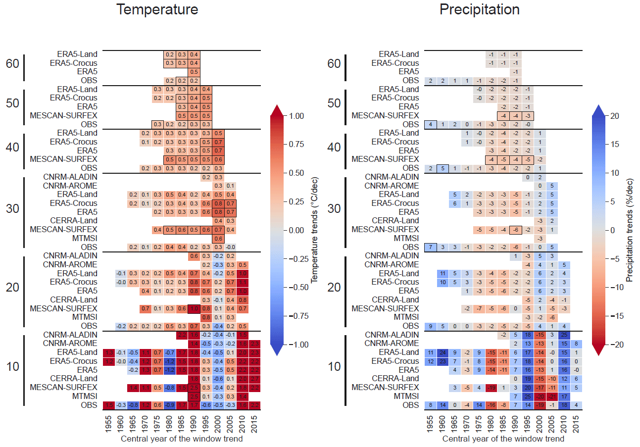
Figure 12 Winter (November–April) trend values for the whole European Alps calculated using Theil–Sen linear regression for two variables (temperature and precipitation). The horizontal axis shows the central year used for the computation of the trend values. The vertical axis provides the series of datasets used for various lengths of the window time periods (10, 20, 30, 40, 50 and 60 years) used for the computation of the trend values. A black-framed square indicates a trend detected as being statistically significant (confidence interval at 95 % excludes zero). Precipitation trends are expressed as relative (% per decade) decrease or increase compared to the mean of the period, while temperature trends are provided as warming rate (^∘C per decade).

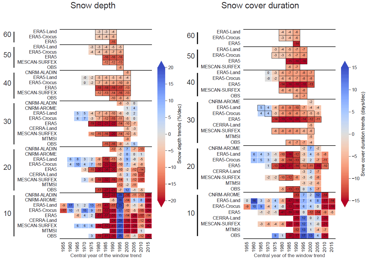
Figure 13 Winter (November–April) trend values for the whole European Alps calculated using Theil–Sen linear regression for two variables (snow depth and snow cover duration). The horizontal axis shows the central year used for the computation of the trend values. The vertical axis provides the series of datasets used for various lengths of the window time period (10, 20, 30, 40, 50 and 60 years) used for the computation of the trend values. A black-framed square indicates a trend detected as being statistically significant. Snow depth trends are expressed as relative (% per decade) decrease or increase compared to the mean of the period, while snow cover duration trends are provided in days per decade (d per decade).

3.3.3 Elevation-dependent climate change (EDCC) and spatial variability in the trends over the 1968–2017 period

The following analyses are dedicated to the spatial variability in the trends: their elevational gradients and their spatial distribution. Trends are calculated over the 1968–2017 period using the available datasets for this time period: OBS (i.e., in situ observations of snow depth for the mean winter snow depth and snow cover duration: E-OBS v19.0HOM for the winter temperature and LAPrec for the winter precipitation), ERA5, ERA5-Land, ERA5-Crocus and MESCAN-SURFEX. The choice of a window length of 50 years relies on the analyses presented in Sect. 3.3.2, showing that at least 40 years is the minimum time duration required to get a consistent signal at the scale of the entire Alps.

Winter temperature trends in Figs. 14 and 15 show different spatial patterns depending on the dataset. E-OBS v19.0HOM, here taken as the reference, displays a rather smooth winter temperature trend field in Fig. 15 with most of the trends detected as being significant (i.e., non-hatched areas). Not surprisingly, the three ERA5 products show similar patterns with higher warming rates ranging from 0.5 to 1.0 ^∘C per decade in the eastern half of the Alps, and all were detected as being significant compared to the lower trends (i.e., below 0.4 ^∘C per decade) elsewhere. MESCAN-SURFEX exhibits the highest warming rates, with stronger values over the Alpine ridge, corresponding to higher-elevation areas, which can also be noticed in the boxplot in Fig. 14 through the strong elevational gradient. Given the amplitude of the elevational gradient simulated by MESCAN-SURFEX above 1500 m (i.e., median shifted by 0.5 ^∘C per decade per 1000 m), as well as the fact that the other datasets agree more on a slightly decreasing elevational gradient at these elevations similar to what Rottler et al. (2019) found over the Swiss Alps for the 1981–2017 period, MESCAN-SURFEX behaviors may be considered spurious artifacts.

Winter precipitation trends are weak for all datasets except for MESCAN-SURFEX. For the reference and the three ERA5 products, spatial patterns are similar in Fig. 15, with a widespread light decrease in precipitation, higher in the western part of the Alps but still lower than 7 % (not detected significant), and no elevational gradient in Fig. 14. The MESCAN-SURFEX trend field in Fig. 15 shows larger values, exceeding ±15 % per decade with a patchy appearance (i.e., alternating strong positive/negative values) and a strong elevational gradient, both more reminiscent of artifacts than a realistic pattern.

Snow variables (i.e., snow cover duration and mean winter snow depth) present similar geographical patterns (see Fig. 15). ERA5-Land and ERA5-Crocus expose a rather similar decline in both variables: a bit stronger in the southern and in the eastern parts of the Alps. The decrease is around −10 % per decade and −7 d per decade, respectively, for the mean winter snow depth and the snow cover duration, values that are close to the ones given as reference using the set of in situ observations. As shown above in Sect. 3.3.2, ERA5 displays spurious values, almost twice the reference values, that we link to a heterogenous assimilation procedures that have corrected an overly thick modeled snowpack over the last decades, artificially reinforcing the decreasing trend. MESCAN-SURFEX snow variable trend fields show similar patterns to its precipitation trend field, with a patchy field displaying a strong horizontal gradient, probably inherited from the precipitation field. Concerning the elevational gradient in Fig. 14, all datasets are in broad agreement for both variables. They simulate a stronger relative decline of the mean winter snow depth at low elevations, decreasing with the altitude. Snow cover duration trends also present a weak elevational gradient for all the datasets, with a stronger decline at low and intermediate elevations and with a median near −7 d per decade compared to the −5 d per decade at high elevations for ERA5-Land, ERA5-Crocus, MESCAN-SURFEX and the reference. The highest changes in snow conditions at low and intermediate elevations (near the snowline) have already been documented in multiple studies. Indeed, the Kuhn and Olefs (2020) review of EDCC over the European Alps shows that the decline of both snow cover duration and snow depth over the 1961–2018 period is linearly related to elevations (i.e., with a stronger decline at low and intermediate elevations).

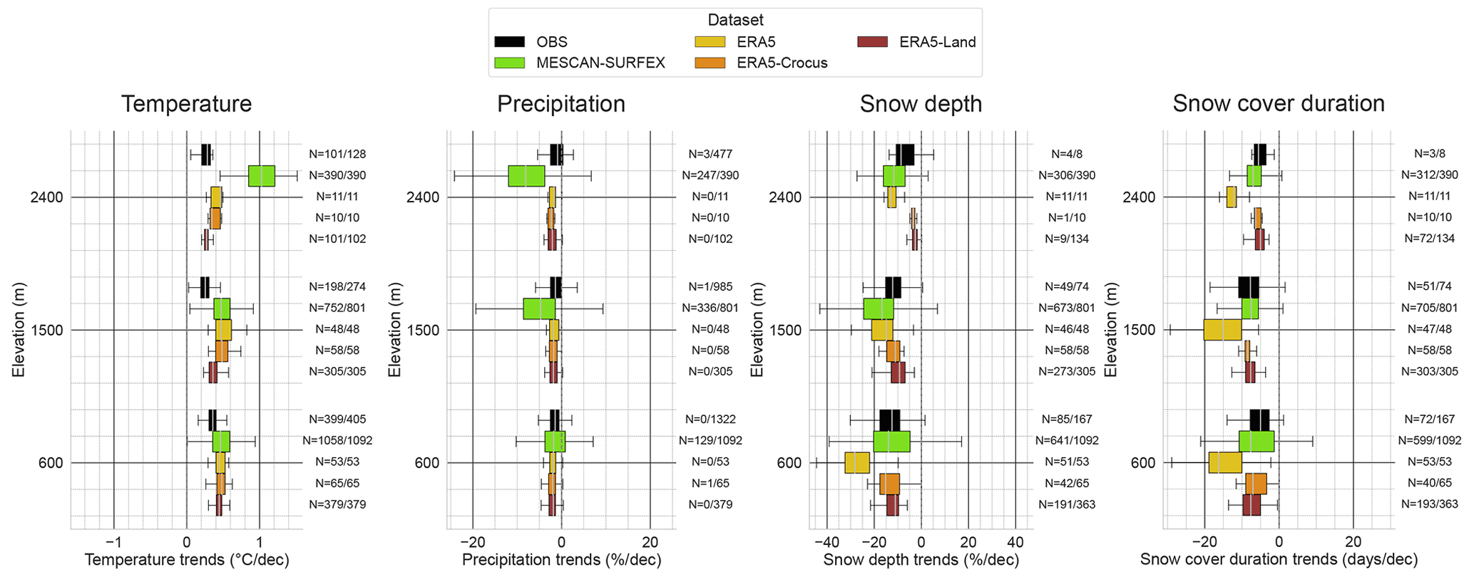
Figure 14 Boxplot of the winter (November–April) trend values calculated over the 1968–2017 period (50 years) for each grid point of the entire Alps (grid points included within the 450–2550 m elevation range) using Theil–Sen linear regression for four variables (temperature, precipitation, snow depth and snow cover duration). For this length of the period, five datasets are available: observations (E-OBS v19.0HOM for temperature, LAPrec for precipitation, and the set of in situ observations for snow depth and snow cover duration), MESCAN-SURFEX, ERA5, ERA5-Land and ERA5-Crocus. Precipitation and snow depth trends are expressed as relative (% per decade) decrease or increase compared to the mean of the period, while temperature and snow cover duration trends are provided as absolute rate. The N number represents the number of trends detected as being significant out of the total number of trends calculated.

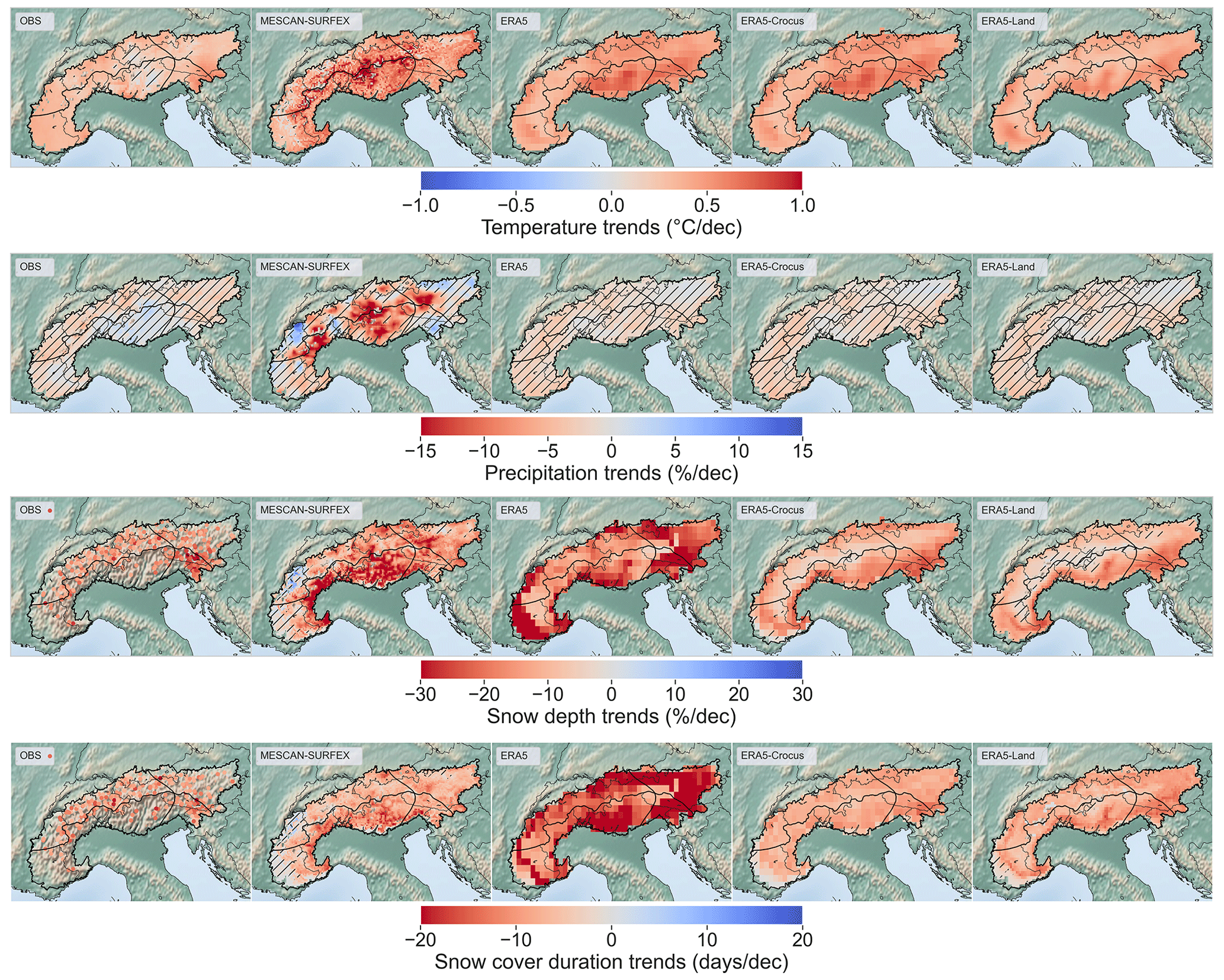
Figure 15 Maps of the winter (November–April) trend values calculated over the 1968–2017 period (50 years) for each grid point of the entire Alps (grid points included for three elevation bands (±150 m) given on the y axis) using Theil–Sen linear regression for four variables (temperature, precipitation, snow depth and snow cover duration). Non-hatched areas indicate trends detected as being statistically significant (i.e., p value of the Mann–Kendall test below 0.05). Precipitation and snow depth trends are expressed as relative (% per decade) decrease or increase compared to the mean of the period, while temperature and snow cover duration trends are provided as warming rate (d per decade).

4 Discussion

In this study, we have compared the results of various modeling systems (global and regional reanalyses and regional climate model simulations driven by a global reanalysis) against observation references (in situ, kriged datasets and satellite observation). The comparisons are performed in terms of monthly and seasonal snow depth values, snow cover duration, snow onset date, and snow melt-out date, addressing multi-annual averages of regional and subregional mean values, their interannual variations, and trends over various timescales. Here we discuss the main findings of the study and draw implications for further use of these datasets in various contexts. Remember that this study investigates mean seasonal to monthly snow characteristics and their main driving variables (temperature and precipitation) at the scale of the European Alps and for four subregions. The diversity of the datasets involved in this study and the difficulties of carrying an unbiased point-scale (station vs. grid points) comparison over mountainous terrain (i.e., due to the scarcity of the observations and to the strong horizontal gradients) led us to constrain the investigation to statistics over large areas. Consequently, the study does not address the characteristics of the datasets at local scale, and these may differ from their large-scale characteristics.

4.1 Snow cover characteristics as seen by different modeling systems

This subsection is dedicated to the discussion of the different behaviors of the datasets concerning the snow conditions, characterized by snow depth, snow cover duration, snow onset date and snow melt-out date.

Compared to the observational references, the worst performances (lowest scores and strongest deviations from the reference) concerning the representation of the snow characteristics are obtained with ERA5-Land, CNRM-AROME and CNRM-ALADIN. CNRM-AROME and ERA5-Land both overestimate the snow depth, the snow season lasts too long (about 1 month later than the other datasets), and there are areas with spurious snow accumulation above 2000 m. For CNRM-AROME, these issues have already been documented by Monteiro et al. (2022) over the French Alps; the finding also applies at the scale of the European Alps. Monteiro et al. (2022) attributed these issues to the deficiencies of the snow scheme physics (i.e., missing processes that lead to an underestimated melt), along with a biased surface energy balance related to both a misrepresentation of surface–atmosphere exchanges and the underestimation of upwelling infrared radiation (due to the underestimation of nighttime cloud cover). Muñoz-Sabater et al. (2021) evaluated snow depth results of ERA5-Land and ERA5 against in situ snow depth observations, mainly in the Rocky Mountains (western US). They do not report any snow accumulation issues at high elevations, and for low and intermediate elevations, ERA5-Land shows a lower mean absolute error compared to ERA5. In their study, only 30 observation points were used in the European Alps, and they show a higher mean absolute error in ERA5-Land results compared to ERA5, in line with our analyses. This was interpreted as an effect of the dense SYNOP (surface synoptic) observation network incorporated in the snow assimilation system of ERA5, allowing it to perform better than ERA5-Land over this region. Compared to CNRM-AROME, at a regional to subregional scale, no strong overestimation of precipitation was shown in ERA5-Land, which could explain the spurious accumulation of snow, but they have in common the use of a single-layer snow scheme and a strong negative temperature difference in winter.

The simplicity of these snow schemes, through the underestimation of melting processes, along with atmospherical forcing leading to too much snow accumulation (likely overestimation of winter/spring precipitation) and weaker melting conditions (underestimation of winter/spring temperatures and erroneous surface mass balance), could explain part of the observed differences in snow depth values compared to the reference observations. Despite the use of the same snow scheme, it is likely that these errors are strongly reduced in ERA5 thanks to the data assimilation of snow depth observations. Orsolini et al. (2019) showed that over the Tibetan Plateau where no observations of snow depth are assimilated, ERA5 strongly overestimates the snow cover and the snow depth and attributes part of it to the overestimation of snowfall. These give us evidence that assimilation (snow depth but also precipitation and near-surface temperature) potentially strongly benefits the ERA5 results in the European Alps. In ERA5-Crocus, the use of a detailed representation of the snowpack within the Crocus snow model is intended to provide a better representation of the accumulation and melting processes. ERA5 and ERA5-Crocus, potentially for different reasons, provide snow depth values and simulate a seasonality of the snowpack closer to the reference snow cover than ERA5-Land, although with a coarser horizontal resolution.

The combination of a strong negative temperature bias in CNRM-ALADIN and its strong overestimation of winter precipitation (already identified by Terzago et al., 2017, and common to numerous regional climate models of EURO-CORDEX) is a possible explanation for the overestimation of snow accumulation at the beginning of the season for intermediate- and high-elevation bands. While the negative temperature bias should favor late melting, the opposite phenomenon is observed, which points towards other problems with the snow schemes and would require additional sensitivity studies to precisely identify the causes.

The regional reanalyses MESCAN-SURFEX, CERRA and MTMSI provide snow depth values and snow seasonality closest to the reference. Although they do not assimilate snow depth values, it appears that their surface analysis through the MESCAN system provides reliable snow cover first-order atmospherical drivers (precipitation and temperature) along with a fair representation of the snow physics within ISBA-ES or Crocus.

Overall, our analysis finds that there are multiple combinations of atmospheric and land surface modeling systems (Essery et al., 2020; Menard et al., 2020) and their corresponding data assimilation frameworks (or not), leading to various snow cover datasets generated through numerical modeling. The performance of these datasets vary, and none are found to be totally irrelevant for the variables analyzed in this study. However, no system is found to outperform all of the other ones in all of the dimensions of the evaluation, which can also be traced to the fact that none of the currently available systems combine the “best” of all worlds (high resolution, sufficiently sophisticated snow cover model well adapted to the land surface model, surface data assimilation including precipitation, snow cover data assimilation, etc.).

4.2 On the complexity of assessing differences between modeling systems

In addition to the general discussion provided above, here we insist that the comparison between all of the evaluated datasets, and in particular the three ERA5 datasets and CNRM-AROME, is not straightforward. Even if ERA5 and ERA5-Land have in common their land surface model and snow scheme configuration, ERA5-Land does not simulate the feedback from the surface to the atmosphere at its resolution, while ERA5 is constrained by a large number of observations through its land data assimilation system. ERA-Crocus is run in standalone mode too, but the configuration of the land surface snow scheme is somewhat specific (e.g., it considers a fully snow-covered surface even if only a thin layer (i.e., 10 cm) of snow is presents). CNRM-AROME shares a rather similar single-layer snow scheme to ERA5-Land and ERA5 but simulates a coupling with near-surface atmosphere without assimilating any observations. Finally, CHTESSEL (for ERA5 and ERA5-Land) and SURFEX (for CNRM-AROME, ERA5-Crocus) are two different land surface models, based upon different ways of taking into account the presence of snow over the surface, particularly its impact on energy balance calculations. This implies a wide range of responses of the different snow schemes (notably according to their complexities) for atmospheric forcings that can be of very variable quality as underlined by Terzago et al. (2020). Furthermore, even in the case of a similar configuration of the model's atmospheric components, different configurations of the same snow scheme are generally possible and can lead to large differences in the simulated snowpack (Lafaysse et al., 2017; Napoly et al., 2020). Thus, a clear attribution of the different factors conducive to the different behaviors of the modeling systems turns out to be virtually impossible in the absence of an extensive sensitivity study to apportion the contribution of each possible factor, which is beyond the scope of this study (and may remain an elusive goal due to the complexity involved in disentangling such complex modeling frameworks).

4.3 Representation of the interannual variability

The study of the interannual variability in the snow conditions through two variables, the mean winter snow depth and the annual snow cover duration, as well as their main driving variables (near-surface temperature and precipitation), sheds light on multiple aspects of the variability in the snow conditions in the European Alps.

Near-surface winter temperature anomalies are rather homogenous among the different subregions with a small subregional variability, meaning that most of the interannual variability affects the whole Alpine region similarly. All datasets reproduce correctly the anomalies compared to the reference, and even if no strong discrepancies are found between them, climate simulations (CNRM-AROME and CNRM-ALADIN), CERRA-Land and ERA5-Land perform better than ERA5, MTMSI and MESCAN-SURFEX.

Winter precipitation shows a strong subregional variability, varying from ±50 % from one year to the next but rather similarly inside a given subregion. This is coherent with past classifications such as HISTALP (Auer et al., 2007), making winter precipitation vary for a significant part independently from one subregion to the others. On these anomalies, datasets only show little discrepancies with LAPrec taken as reference, and no dataset outperforms the others in every subregion.

Mean winter snow depth and snow cover duration show the largest interannual variabilities across and within subregions of the European Alps. Datasets show the lowest correlation scores with the reference value, with a generalized underestimation of the amplitude of the interannual variability. In fact, both indicators are influenced by a large set of components (temperature, precipitation, wind, radiation, etc.) and result from the integration, over the course of the winter season, of many processes operating at multiple space scales and timescales. These contribute to widening the discrepancies concerning the snowpack characteristics between locations nearby all throughout the winter periods and increase the interannual variability at a very local scale. Additionally, the accuracy of precipitation and temperature fields throughout the snow season, as well as the snowpack modeling system, is widely different across the datasets, and this ultimately determines a large fraction of the quality of the simulated snow depth time series. Overall, these analyses demonstrate that the snowpack interannual variability is still challenging to simulate, and as the interannual variability in precipitation and air temperature is already rather well represented according to our analysis, efforts might be directed towards the improvement of the snow modeling framework.

4.4 Reliability of the trend values

The analysis of mean winter values at the scale of the entire Alps assessed in Sect. 3.3.2 confirmed that detecting a trend needs to be done cautiously. First of all, our analysis confirms that trends analyzed over time periods that are too short (typically, less than 30 years) are prone to large errors and the influence of decadal climate variability. This is illustrated in Fig. 13, which confirms that, in particular, snow cover trends analyzed over the past 20 years only cannot be considered representative of longer-term climate trends. As a consequence, key data records, such as satellite observations, which only cover such a limited time span, should be used with special care when they are used for trend analysis because this could lead to erroneous results. Instead, our study shows that there is potential to use satellite information together with other sources of information (in situ, numerical simulation and their combination) to overcome the time resolution and target variables conundrum (Gascoin et al., 2022).

In addition to this reminder on some key safeguarding principles related to the calculations of snow cover trends, this analysis bears some relevance with respect to the sources of variability and trends for snow cover variables in mountain regions. Indeed, the different variables investigated are affected at different timescales (i.e., from annual to multi-decadal) by fluctuations that can alternatively favor particular climate conditions (e.g., warm and dry or cold and wet conditions). These oscillations of the climate system generally occur at a larger scale than the European Alps and can be described through modes of variability. The two main modes that affect the variables investigated here on the European Alps are the North Atlantic Oscillation (NAO) and the Atlantic Multi-decadal Oscillation (AMO or AMV) (Cassou et al., 2021). They typically favor winter and in their positive phase warmer and wetter conditions for the NAO and colder and wetter conditions for the AMO, implying a potentially strong influence on the snowpack evolution (Scherrer and Appenzeller, 2006; Durand et al., 2009). However, while a relationship between past decreases in spring precipitation in the southern Alps and the positive phase of the AMO has been reported (Brugnara and Maugeri, 2019), as well as winter precipitation in the western Italian Alps with the NAO (Terzago et al., 2013), to our knowledge, only a few studies have attempted to link snow conditions in the European Alps to large-scale modes of variability (NAO, AMO, El Niño–Southern Oscillation – ENSO, etc.). Due to the low amplitudes of these oscillations and the large number of superimposed factors affecting the snowpack at different spatiotemporal scales, no clear consensus has been found so far. Overall, our analyses show that below 30- to 40-year time lengths, many of the trends are not detected as being significant and can fluctuate between strong negative or positive values for consecutive time periods. Beyond 40-year window lengths, the signal-to-noise ratio becomes larger and can lead to the detection of meaningful and significant changes in the mean values.

This study also brought to light artifacts affecting the trends held by datasets incorporating information from observations. ERA5 (and to a lesser extent ERA5-Land) and MESCAN-SURFEX winter temperature trends are systematically overestimated compared to the reference E-OBS and past studies. Figures 14 and 15 show that in the case of ERA5 products, warming is particularly overestimated in the eastern part of the Alps, whereas MESCAN-SURFEX simulated a much stronger warming at high elevations, leading to a spurious elevation-dependent warming. Similarly, MESCAN-SURFEX winter precipitation trend fields display an unrealistic geographical distribution of values associated with strongly overestimated amplitudes. These spurious precipitation trends are reflected in comparable snow depth and snow cover duration trend fields and are also overestimated. Finally, ERA5 snow depth and particularly snow cover duration trends are strongly overestimated (twice the amplitudes of the reference).

These behaviors point at least in part to a common cause: the assimilation of a varying (in quantity and in quality) number of observations over time that better correct model biases in spaces and times where observations are dense. This leads to a shift in the distribution of a variable, therefore inducing artificial trends.

ERA5 and MESCAN-SURFEX are based on modeling strategies that favor the maximization of the agreement between model and observations at the expense of temporal consistency, which would better enable the product to be used for trend assessment.

Users of these products should therefore be aware of the limits of the quality of a dataset incorporating information from observations. As reminded by Cornes et al. (2018), Kaiser-Weiss et al. (2019), and Bandhauer et al. (2022), their quality highly varies depending on the spatiotemporal scale considered (i.e., their effective resolutions) and the areas considered, both of which are strongly affected by the density of the observations used in the product. In addition, the use of a heterogenous number of observations can lead to a differential correction of the products over time, inducing artificial trends within it, as we see here for the Alps with MESCAN-SURFEX winter precipitation trends or ERA5 snow variables.

5 Conclusions

In this study, we investigate the ability of various modeling systems (global and regional reanalyses and regional climate model simulations driven by a global reanalysis) to represent past snow conditions and the main atmospherical drivers over the European Alps, using observational references (in situ, kriged datasets and satellite observation). The comparisons are performed in terms of monthly and seasonal values, addressing multi-annual averages of regional and subregional mean values, their interannual variations, and trends over various timescales.

The comparisons of the datasets over a common period of 30 years (1985–2015), in terms of the average of monthly and seasonal values of the snow depth and snow cover duration at a regional scale, shed light on a variety of behaviors that can lead to strong differences between the evaluated and the reference datasets. ERA5, ERA5-Crocus, CERRA-Land, UERRA MESCAN-SURFEX and MTMSI simulate a monthly evolution of the snow rather close to the reference, at a regional and subregional scale, with no dataset systematically outperforming the others. CNRM-AROME and ERA5-Land are both found to overestimate the amount of snow and its persistence throughout the snow season, a phenomenon that increases with elevation, leading to spurious snow accumulation above 2000 m. CNRM-ALADIN shows an overestimated accumulation of snow at the beginning of the season and a total melt that occurs about 1 month earlier than the reference dataset for elevations above 1500 m.

The spatial comparison against MODIS remote sensing data supports what appears to be a common issue of all datasets, namely the overestimation of the snow cover duration above 1000 m, with stronger errors near the snow line (around 1500 m) and concentrated on the melt-out date.

The discrepancies concerning the past climatology of snow conditions found between the reference and evaluated datasets may have multiple sources, affecting each of the datasets differently, and we can only hypothesize them here. Indeed, setting a clear attribution of the different factors leading to the different behaviors of the modeling systems would required multiple extensive sensitivity studies addressing independently the impact of multiple error sources. Among the various plausible factors, we suspect biases from the atmospherical forcings, limitations of land surface data assimilation procedures for mountainous areas, and the misrepresentation of surface–atmosphere exchange and key snow processes (i.e., wind-transport, glacier accumulation), along with potentially inadequate configurations of the snow schemes leading to erroneous melt rate.

The study also addresses the representation of the interannual variability by the different evaluated datasets and their simulated trends over various timescales. Temperature and precipitation interannual variabilities are found to be rather well represented by most of the datasets. However, the simulation of the interannual variability in snow cover variables appears to remain difficult for all datasets. Their lowest performance may come from several causes related to the difficulty of representing the strong variance of the interannual fluctuations and the local variability in the snow conditions. This may be due partly to misrepresented processes related to the problems mentioned above and to the specificity and the complexity of the modeling of the snowpack. We mention that snow variables are somehow specific, as they result from a cumulative history all throughout the snow season. Therefore, errors from atmospherical forcings, snow modeling, and coupling between surface–atmosphere and assimilation also cumulate over time.

The computation of trends over various timescales leads us to reiterate some safeguarding principles on the matter. Indeed, computing trends over timescales shorter than 30 years results in the detection of noisy signals, strongly affected by interannual to multi-decadal variability and often not statistically robust. In addition, some datasets (MESCAN-SURFEX and CERRA-Land for precipitation and snow variables and ERA5 for snow variables only) lead to spurious trends (i.e., strongly overestimated amplitudes and incoherent geographical patterns even for long-term trends), probably induced by spatiotemporal heterogeneities in their assimilation procedures. These datasets should be used carefully for climate change applications as some of the simulated variables may be affected by artifacts, impacting the reliability of the resulting trends.

Overall, no dataset outperforms the other in terms of the multiple aspects investigated here. Upstream modeling choices have indeed great consequences on the downstream uses of these datasets. Reanalyses (and datasets based upon observation sources) hold the potential to partially fulfill the gap of in situ observations in mountainous areas and provide a consistent and reliable baseline of the key variables describing the evolution of climate conditions in mountainous areas. Nonetheless, we find that the quality of these datasets is scale and location dependent. As mentioned by Isotta et al. (2015), Kaiser-Weiss et al. (2019), and Bandhauer et al. (2022), the quality of the datasets incorporating observations (using assimilation procedures or direct kriging method) is strongly dependent upon the density of the observations used (and their spatiotemporal homogeneity), and the effective resolution of these datasets is in fact generally lower than the provided grid resolution. In mountainous regions the scarcity of observations remains a strong obstacle, and standard assimilation techniques can lead to a deterioration in the quality of simulated fields, as the spatial variability is high over mountainous areas, and the influence of an observation should be restrained to its domain of applicability (same elevation, slope, aspect, etc.). Furthermore, observation-based products (including reanalyses) necessarily result from a trade-off between reproducing a climatically relevant time evolution and using the maximum number of available observations to produce the best possible description of the state of the atmosphere and snow cover at any given time. Ultimately, this type of dataset continues to rely on the density and quality of the past observational network, which cannot be extended retrospectively. Here we also evaluated the regional climate simulations driven by a robust larger-scale (global) reanalysis. Our results indicate that this can offer an alternative to computationally intensive high-resolution reanalyses for climate studies. Indeed, they can simulate climatically homogenous atmospherical and surface conditions (depending on the quality of the driving, larger-scale reanalysis) and even provide an estimate of the modeling uncertainties if combined with a set of simulations from different regional climate models, although they do not directly incorporate high-resolution data through a data assimilation framework. However, our study shows that for mountain regions several issues with such models need to be tackled. In particular, be it for high-resolution climate modeling or numerical weather prediction models used for the production of reanalyses, investigations into the behavior of the snow cover scheme (and their broader relationship with the rest of the land surface models interacting with the atmosphere) are crucially required. This will hopefully enable us to address these issues in forthcoming versions of these modeling systems.

Appendix A: Reference characteristics of the snow cover in the European Alps

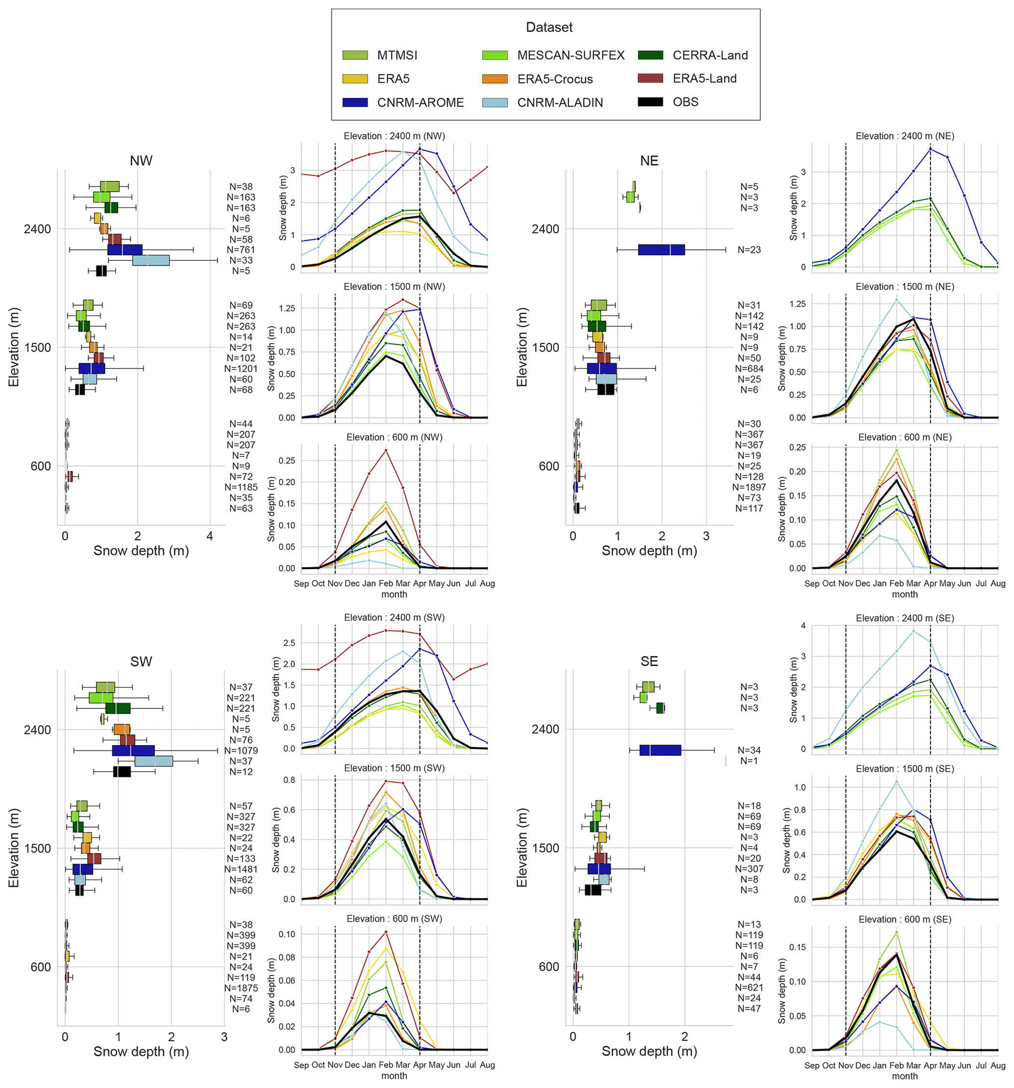
Figure A1 For each subregion of the European Alps: boxplot representing the spatial distribution of mean winter season (November to April) snow depth values over the 1985–2015 period for each dataset for three elevation bands (600 m ± 150 m, 1500 m ± 150 m, 2400 m ± 150 m). Annual cycle of the mean monthly snow depth values for the 1985–2015 period for each dataset for three elevation bands (600 m ± 150 m, 1500 m ± 150 m, 2400 m ± 150 m).

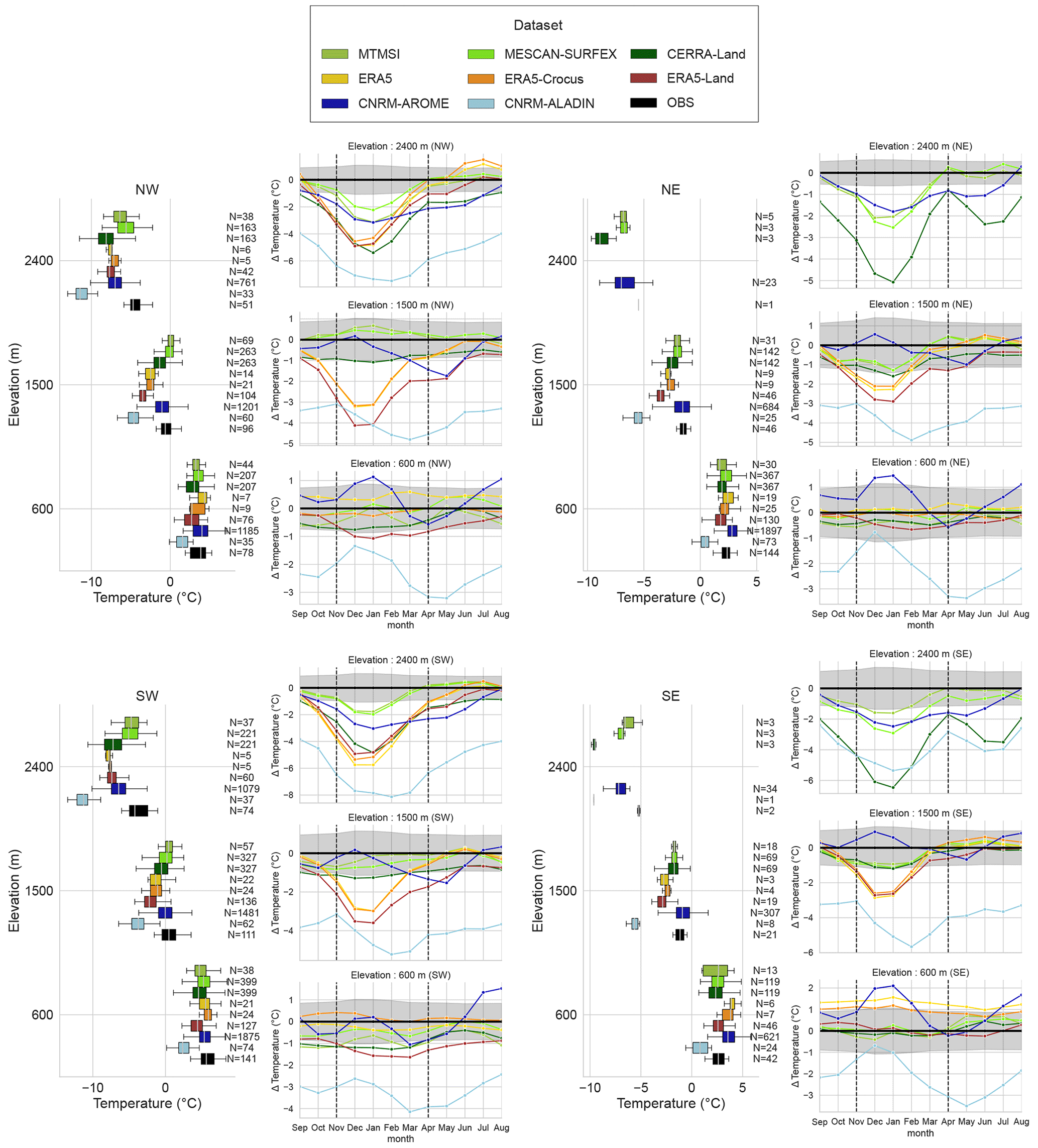
Figure A2 For each subregion of the European Alps: boxplot representing the spatial distribution of mean winter season (November to April) temperature values over the 1985–2015 period for each dataset for three elevation bands (600 m ± 150 m, 1500 m ± 150 m, 2400 m ± 150 m). Annual cycle of the mean monthly error values of temperature for the 1985–2015 period for each dataset for three elevation bands (600 m ± 150 m, 1500 m ± 150 m, 2400 m ± 150 m).

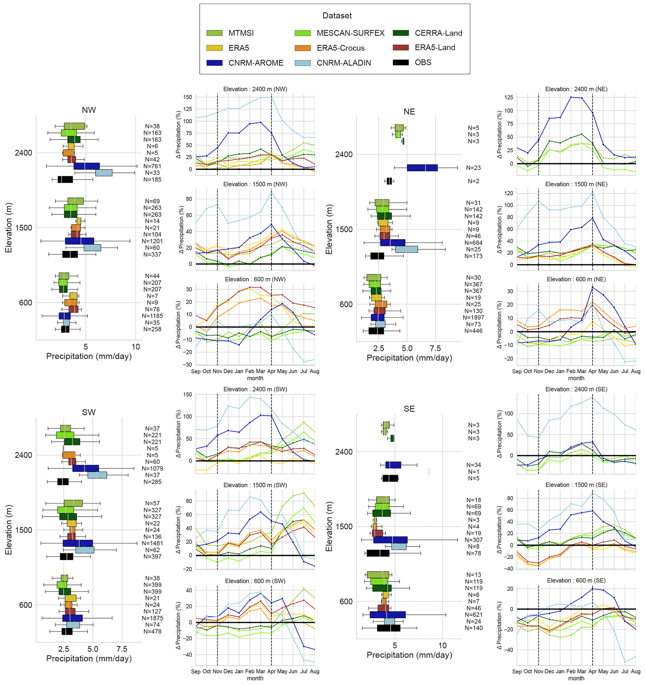
Figure A3 For each subregion of the European Alps: boxplot representing the spatial distribution of mean winter season (November to April) precipitation values over the 1985–2015 period for each dataset for three elevation bands (600 m ± 150 m, 1500 m ± 150 m, 2400 m ± 150 m). Annual cycle of the mean monthly error values of precipitation for the 1985–2015 period for each dataset for three elevation bands (600 m ± 150 m, 1500 m ± 150 m, 2400 m ± 150 m).

Appendix B: Interannual variability

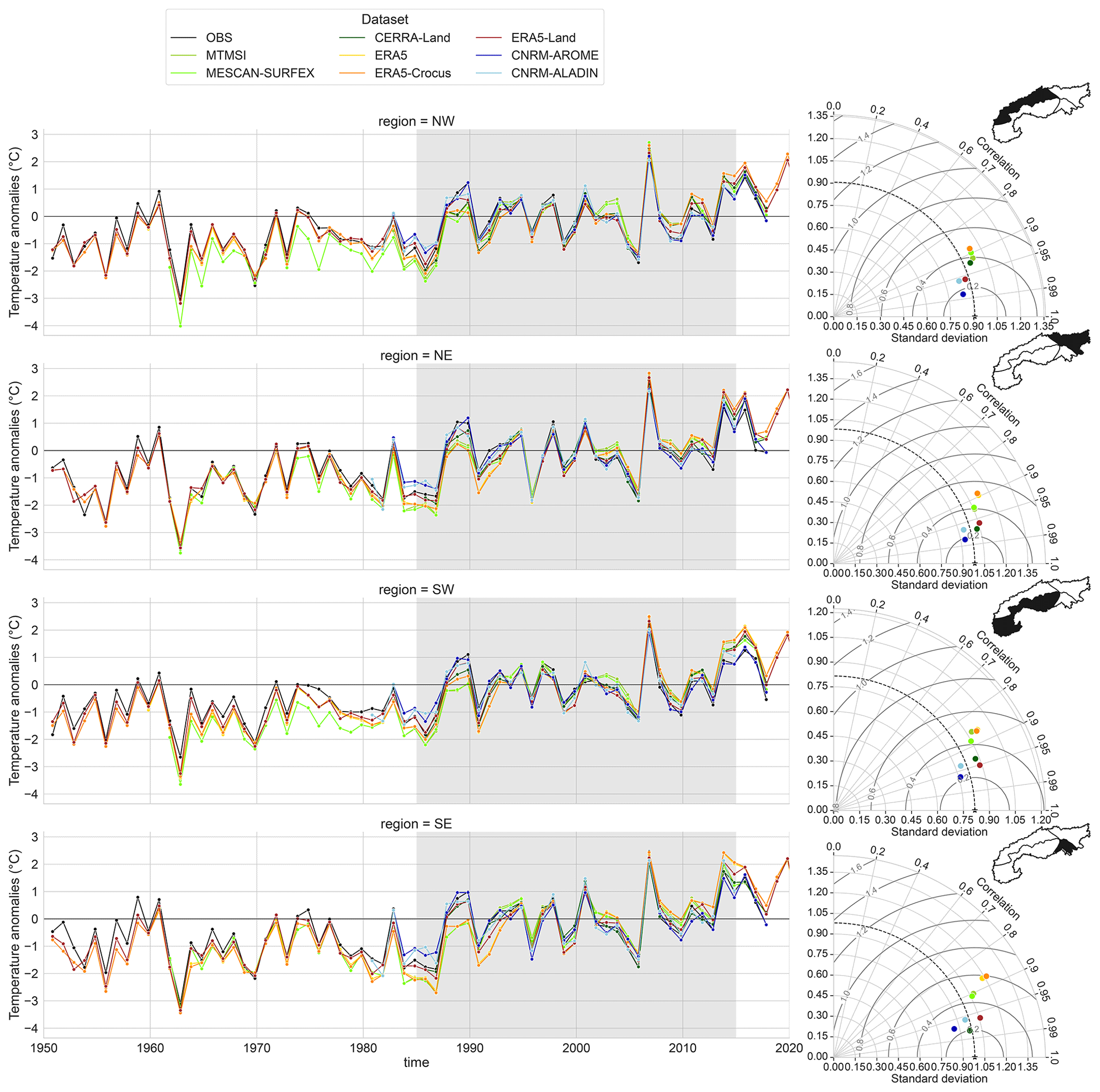
Figure B1 Anomalies of mean winter (November to April) values of temperature in the European Alps for the whole available time period for each dataset compared to the mean winter values of the 1985–2015 period (shaded area). On the right, Taylor diagrams calculated using the anomalies of winter values of temperature for the 1985–2015 period (shaded area). The reference used is described in Sect. 2.3.1.

Figure B2 Same as Fig. B1 but for precipitation.

Figure B3 Same as Fig. B1 but for snow depth.

Figure B4 Same as Fig. B1 but for snow cover duration (SCD).

Appendix C: Trends

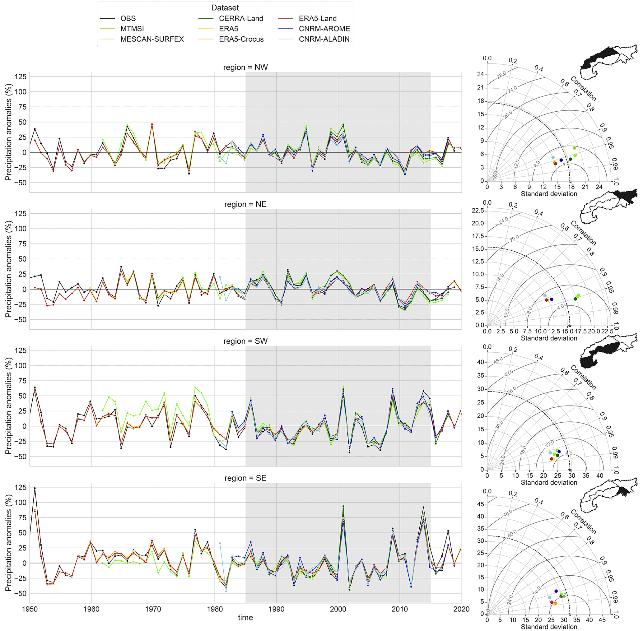
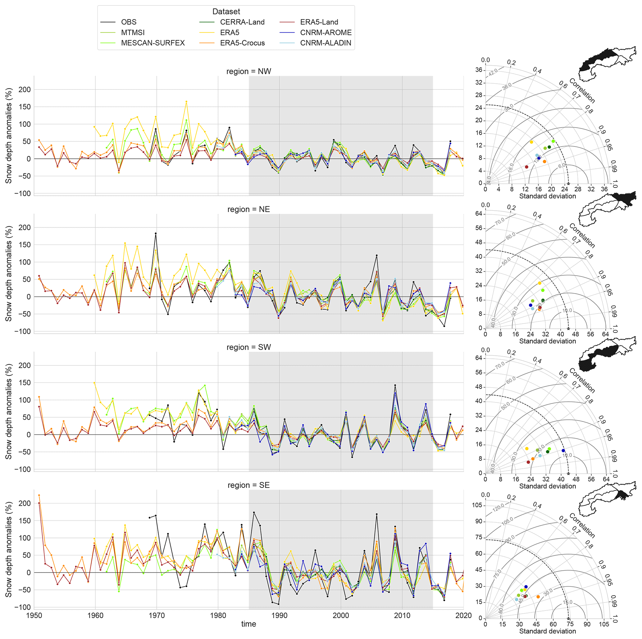
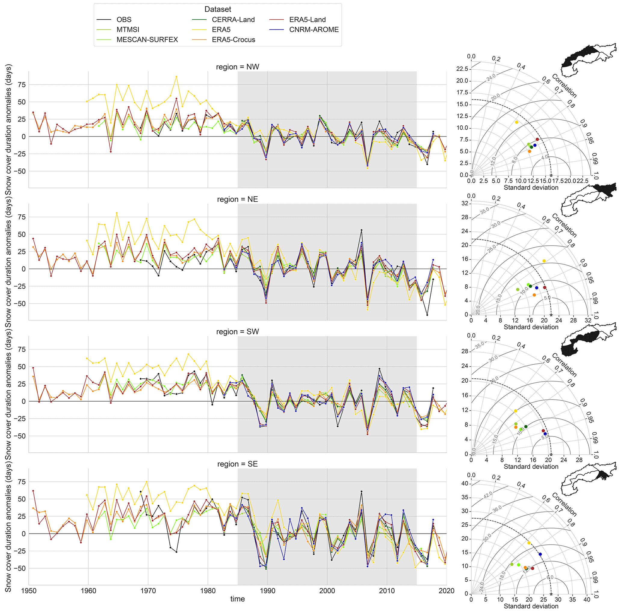
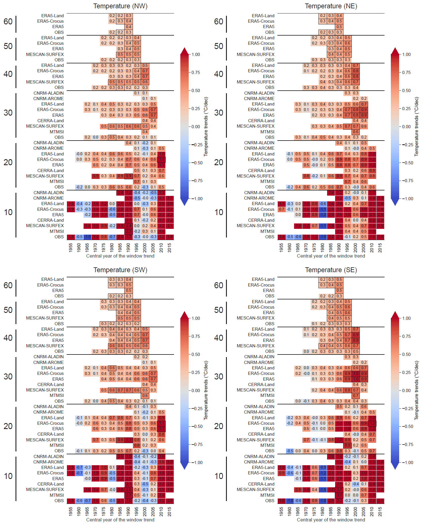
Figure C1 Winter trend values for each subregion of the European Alps calculated using Theil–Sen linear regression for the air temperature at 2 m. The horizontal axis shows the central year used for the computation of the trend values. The vertical axis provides the series of datasets used for various lengths of the window time period (10, 20, 30, 40, 50 and 60 years) used for the computation of the trend values. A black-framed square indicates a trend detected as being statistically significant. Trends are provided as warming rate per decade (^∘C per decade).

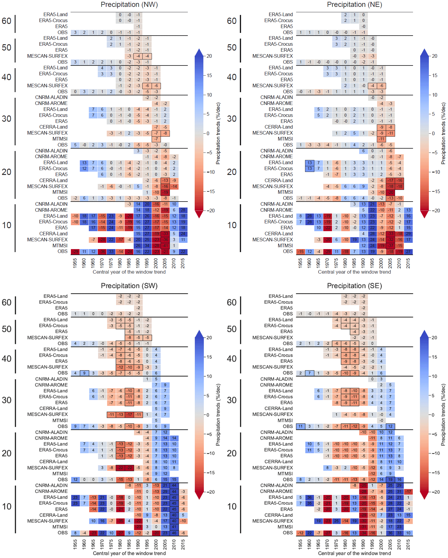
Figure C2 Winter trend values for each subregion of the European Alps calculated using Theil–Sen linear regression for the precipitation. The horizontal axis shows the central year used for the computation of the trend values. The vertical axis provides the series of datasets used for various lengths of the window time period (10, 20, 30, 40, 50 and 60 years) used for the computation of the trend values. A black-framed square indicates a trend detected as being statistically significant. Trends are provided in relative rate per decade (% per decade).

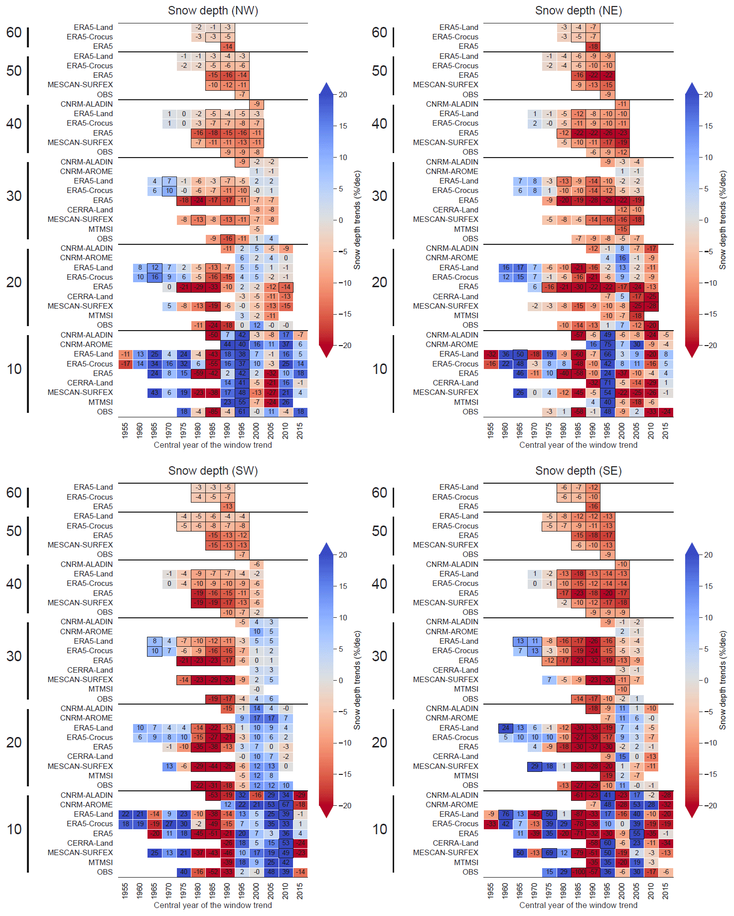
Figure C3 Winter trend values for each subregion of the European Alps calculated using Theil–Sen linear regression for the snow depth. The horizontal axis shows the central year used for the computation of the trend values. The vertical axis provides the series of datasets used for various lengths of the window time period (10, 20, 30, 40, 50 and 60 years) used for the computation of the trend values. A black-framed square indicates a trend detected as being statistically significant. Trends are provided in relative rate per decade (% per decade).

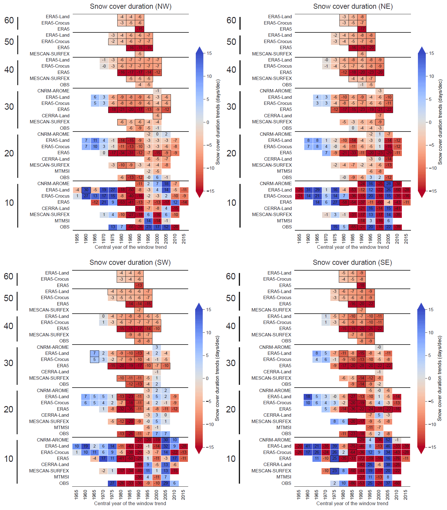
Figure C4 Winter trend values for each subregion of the European Alps calculated using Theil–Sen linear regression for the snow cover duration. The horizontal axis shows the central year used for the computation of the trend values. The vertical axis provides the series of datasets used for various lengths of the window time period (10, 20, 30, 40, 50 and 60 years) used for the computation of the trend values. A black-framed square indicates a trend detected as being statistically significant. Trends are provided in days per decade (d per decade).