the Creative Commons Attribution 4.0 License.
the Creative Commons Attribution 4.0 License.
 | 25 Aug 2023
Summer sea ice floe perimeter density in the Arctic: high-resolution optical satellite imagery and model evaluation
Byongjun Hwang
Adam William Bateson
Yevgeny Aksenov
Christopher Horvat
Size distribution of sea ice floes is an important component for sea ice thermodynamic and dynamic processes, particularly in the marginal ice zone. Recently processes related to the floe size distribution (FSD) have been incorporated into sea ice models, but the sparsity of existing observations limits the evaluation of FSD models, thus hindering model improvements. In this study, perimeter density has been applied to characterise the floe size distribution for evaluating three FSD models – the Waves-in-Ice module and Power law Floe Size Distribution (WIPoFSD) model and two branches of a fully prognostic floe size-thickness distribution model: CPOM-FSD and FSDv2-WAVE. These models are evaluated against a new FSD dataset derived from high-resolution satellite imagery in the Arctic. The evaluation shows an overall overestimation of floe perimeter density by the models against the observations. Comparison of the floe perimeter density distribution with the observations shows that the models exhibit a much larger proportion for small floes (radius <10–30 m) but a much smaller proportion for large floes (radius >30–50 m). Observations and the WIPoFSD model both show a negative correlation between sea ice concentration and the floe perimeter density, but the two prognostic models (CPOM-FSD and FSDv2-WAVE) show the opposite pattern. These differences between models and the observations may be attributed to limitations in the observations (e.g. the image resolution is not sufficient to detect small floes) or limitations in the model parameterisations, including the use of a global power-law exponent in the WIPoFSD model as well as too weak a floe welding and enhanced wave fracture in the prognostic models.
- Article
(4535 KB) - Full-text XML
-
Supplement
(3941 KB) - BibTeX
- EndNote


Over the past decades, the extent and concentration of Arctic sea ice have been dramatically declining (Meier et al., 2022). This results in the changing marginal ice zone (MIZ), defined as the ice-covered region affected by waves and swell by the World Meteorological Organization (WMO, 2014). Another alternative definition of MIZ is a sea ice-covered area with sea ice concentration (SIC) of 15 %–80% (e.g. Strong and Rigor, 2013; Aksenov et al., 2017; Rolph et al., 2020; Bateson et al., 2020; Horvat, 2021). Several SIC products are available to define the MIZ, whereas observing waves in sea ice using satellite-derived observations is still an ongoing area of research. Similarly, sea ice modelling studies often do not include an explicit representation of waves in sea ice. Although this SIC-based definition of MIZ is not directly related to the dynamics in this region (Dumont, 2022), due to the lack of techniques for detecting wave–ice interactions (Horvat et al., 2020), this definition has been widely applied in previous studies. One of the major characteristics of the MIZ is the presence of discrete ice floes in different sizes and shapes, forming the floe size distribution (FSD) (Rothrock and Thorndike, 1984).
Previous studies have suggested the FSD is important for sea ice processes in the MIZ. The FSD is linked to the total perimeter of the ice floes in the fragmented sea ice field, which is an important parameter influencing the sea ice melt occurring around the side of floes and ocean eddy processes (Steele, 1992; Tsamados et al., 2015; Arntsen et al., 2015; Horvat et al., 2016). Floe size influences the ocean surface heat budget and affects sea ice rheology (Shen et al., 1986; Feltham, 2005; Rynders, 2017), which in turn can affect lead dynamics. The FSD also affects the atmosphere–ocean momentum transfer (Tsamados et al., 2014). In the MIZ, small ice floes (the diameter <100 m) significantly increase the floe edge contribution to form drag and surface roughness (Steele et al., 1989; Herman, 2010; Lüpkes et al., 2012; Tsamados et al., 2014; Rynders et al., 2018; Brenner et al., 2021). This increases the momentum transfer between the atmosphere and the ocean (Steele et al., 1989; Birnbaum and Lüpkes, 2002; Herman, 2010; Martin et al., 2016). The FSD affects the ocean surface wave propagation and attenuation through the ice; i.e. floes smaller than a characteristic wavelength of swells attenuate wave energy through dissipative processes, while larger floes attenuate the wave energy through scattering (Kohout and Meylan, 2008; Williams et al., 2013a; Thomson and Rogers, 2014; Montiel et al., 2016; Meylan et al., 2021; Dumas-Lefebvre and Dumont, 2023; Horvat and Roach, 2022).
Given the crucial role of the FSD in various processes within the MIZ, a proper treatment of the FSD-related processes has become a key issue in simulating sea ice. Recently FSD parameterisations have been incorporated into sea ice models (Horvat and Tziperman, 2015; Zhang et al., 2016; Bennetts et al., 2017; Rynders, 2017; Roach et al., 2018a; Bateson et al., 2020). For example, current FSD prognostic models consider the FSD evolution driven by thermodynamic and dynamic processes, including lateral melt (Horvat and Tziperman, 2015; Zhang et al., 2015; Roach et al., 2018a), ice ridging and ice fragmentation (Zhang et al., 2015; Horvat and Tziperman, 2015), wave-induced fracture (Horvat and Tziperman, 2015; Bennetts et al., 2017; Roach et al., 2018a), new ice formation (Roach et al., 2018a), floe welding (Roach et al., 2018a), and brittle fracture (Bateson et al., 2022). Some other modelling studies have assumed a particular shape of the FSD (e.g. Bennetts et al., 2017; Rynders, 2017; Bateson et al., 2020). To enhance the understanding of the FSD evolution in various seasons and regions in the Arctic, a wide range of observations from aerial vehicles (e.g. Perovich and Jones, 2014; Toyota et al., 2016); optical satellites, e.g. Landsat (e.g. Rothrock and Thorndike, 1984; Gherardi and Lagomarsino, 2015; Wang et al., 2016); MEDEA (Measurements of Earth Data for Environmental Analysis; e.g. Denton and Timmermans, 2022; Hwang and Wang, 2022); MODIS (Toyota et al., 2016; Stern et al., 2018a); and synthetic-aperture radar (SAR), e.g. TerraSAR-X (Hwang et al., 2017b; Stern et al., 2018a), have been used to derive floe sizes. Previous observational studies reported a power-law behaviour existing in the tail of the FSD, i.e. a straight line in logarithmic axes, leading to the parameterisations of fixing the FSD as a truncated power law (Burroughs and Tebbens, 2001). However, the floe size power-law hypothesis has been contested by recent observations (Steer et al., 2008; Herman, 2010; Herman et al., 2021), which suggest that different shapes or functions can be better at describing FSDs. Results from laboratory experiments (Herman et al., 2018; Passerotti et al., 2022) and models (Herman, 2017; Montiel and Squire, 2017; Mokus and Montiel, 2022; Montiel and Mokus, 2022) indicate that a power-law FSD may be not the most appropriate way to describe the FSD due to wave-induced sea ice breakup.
Accurate model projections of Arctic climate change are needed to guide research and the response to climate change. The development of the FSD models is therefore essential to improve confidence in sea ice models. A major difficulty is the lack of FSD observations, especially high spatial-resolution data to constrain the model parameters and evaluate model performance. Hence, we derived a new FSD dataset from 1 m resolution MEDEA imagery and 0.5 m resolution WorldView imagery products and used the dataset to assess the performance of three selected FSD models. The new FSD data can resolve small floes (up to a few metres), providing a unique opportunity to evaluate the FSD model performance in the Arctic.
In this study, the three FSD models are evaluated against the new FSD dataset. The three models are the diagnostic Waves-in-Ice module and Power law Floe Size Distribution (WIPoFSD) model (e.g. Bateson et al., 2020, 2022) and two fully prognostic FSD models that have branched off from the FSTD model of Roach et al. (2018a, 2019), hereafter FSDv2-WAVE and CPOM-FSD. The FSDv2-WAVE model is developed by Roach et al. (2019), and CPOM-FSD is a branch of this model developed by the Centre for Polar Observation and Modelling (CPOM) with additional features. This paper is organised as follows. The study regions are shown in Sect. 2. In Sect. 3, we introduce the FSD models and the new FSD dataset, and the methods applied to process satellite images to derive the FSD and the metrics used to evaluate the models are described. Section 4 presents the model evaluation results. The discussion and conclusion are given in Sect. 5.
Two study regions were selected for the model evaluation (Fig. 1). The Chukchi Sea region covers an area of 66–80∘ N, 156–180∘ W (blue outline in Fig. 1), and the Fram Strait region covers an area of 77–87∘ N, 20∘ W–20∘ E (red outline in Fig. 1). These regions are where the model outputs were extracted and analysed. The satellite images were acquired over a small area of 70∘ N, 170∘ W in the Chukchi Sea (black dot within the blue outline in Fig. 1) and 84.9∘ N, 0.5∘ E in the Fram Strait region (black dot within the red outline in Fig. 1). The grid cell size of the three models evaluated in this study is 1∘ × 1∘, ranging from 541 km2 for the grid cells near the North Pole to 3802 km2 for the grid cells near the Equator in the study regions. Within every grid cell, the external forcing is homogeneous, and the model accuracy is dependent on the accuracy of external forcing. Compared to the satellite observation, much larger model study regions were selected, which could better represent the inhomogeneous effects of external forcing on the evolution of the FSD and decrease the effects of external forcing bias in a few grid cells on FSDs. In this way, we minimise the bias caused by lower-resolution model outputs than observations and ensure that the model outputs include the ice edge, so better representing the mean state of the FSD in the models. Although both regions represent early-to-late spring sea ice conditions, the observations from the Chukchi Sea region capture a more dynamic and fragmented ice condition (e.g. Fig. 1b), while the observations from the Fram Strait capture a less dynamic environment (e.g. Fig. 1c).
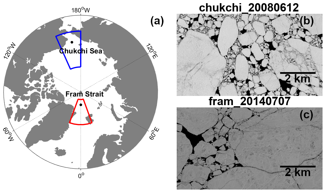
Figure 1(a) Map of the study regions. Satellite images acquired on (b) 12 June 2008 in the Chukchi Sea and (c) 7 July 2014 in the Fram Strait. The blue and red outlines are the boundary of the Chukchi Sea region and the Fram Strait region respectively. The black dots within the study regions mark the locations where satellite imagery data were acquired (70∘ N, 170∘ W in the Chukchi Sea and 84.9∘ N, 0.5∘ E in the Fram Strait).
3.1 Observations
3.1.1 Satellite imagery
In this study we use two types of satellite imagery data. The first is 1 m resolution visual-band panchromatic images provided by the Measurements of Earth Data for Environmental Analysis (MEDEA) group (Kwok and Untersteiner, 2011; Kwok, 2014). The images were accessed from the Global Fiducials Library (GFL) (http://gfl.usgs.gov/, last access: 8 August 2023) of the United States Geological Survey (USGS) and are also known as Literal Image Derived Products (LIDPs). A total of 63 MEDEA images were acquired during May to August over the study period of 2000–2014 at the two fixed locations in the Chukchi Sea and the Fram Strait (Fig. 1). The original MEDEA images of an area larger than 225 km2 (Kwok, 2014) were cropped to remove cloud-covered areas and missing data. The size of the cropped images ranges between 30 and 250 km2 (see Table S2 in the Supplement). We also collected one WorldView-1 (WV1) and four WorldView-2 (WV2) images at the Chukchi Sea and Fram Strait sites (Fig. 1), which are collected in a 50 cm panchromatic band (WV1) at 0.52 m spatial resolution (Satellite Imaging Corporation, WorldView-1 satellite sensor, 2023) and a 50 cm panchromatic band and a 2 m four-band multispectral bundle (WV2) at 0.47 and 0.58 m spatial resolution respectively (Satellite Imaging Corporation, WorldView-2 Satellite Sensor, 2023). The size of the WorldView (WV) images used in this study is ∼ 40 km2.
3.1.2 FSD retrieval from satellite image
Both the MEDEA and the WV images were processed to derive the FSD using the algorithm developed by Hwang et al. (2017a). The algorithm combines speckle filtering, kernel graph cutting (KGC) for the segmentation of water and ice regions, distance transformation, and watershed transformation, a rule-based boundary revalidation to split ice floes boundaries and final manual validation. The minimum size of floes that can be resolved by the algorithm is dependent on the resolution and type of the images. For 1 m resolution MEDEA images, the retrievable floe size ranges between tens of metres to a few kilometres. Small floes with radii smaller than 5 m can be difficult to resolve due to the limitation in splitting the floe boundaries, so the number of small floes is generally underestimated when applying the algorithm to MEDEA images (Hwang et al., 2017a). For the FSD retrieval, we applied the same filter parameter and KGC algorithm parameter as in Hwang et al. (2017b). The SIC was calculated by counting the number of ice pixels out of the total number of image pixels. Segmented water–ice images were then used to split boundaries of sea ice floes using distance transformation and watershed transformation as described by Ren et al. (2015).
3.1.3 Sea ice concentration
Two types of SIC products were used in this study: National Snow and Ice Data Center (NSIDC) SIC of 25 km spatial resolution (Meier et al., 2017; Peng et al., 2013) and the ARTIST Sea Ice (ASI) algorithm 6.25 km SIC (Spreen et al., 2008; Melsheimer and Spreen, 2019, 2020). The collected SIC data cover between May and July during the analysis period of 2000–2014. We note that ASI algorithm SIC is unavailable in April–August 2000–2001, April–May 2002 and April–June 2012. During these periods, we only applied the NSIDC SIC for the model–observation comparison. The SIC data were extracted for the study areas of the Chukchi Sea and the Fram Strait (blue and red outlines in Fig. 1) to compare them with the SIC outputs from the FSD models.
3.2 Sea ice models with floe size distribution
In this study, three FSD models are evaluated. An overview of the configuration of these three FSD models is given in Table 1. In Sects. 3.2.1–3.2.3, we will briefly describe the three models and highlight the major differences between them in simulating the FSD-related processes.
Table 1Summary of model simulations used in this study.
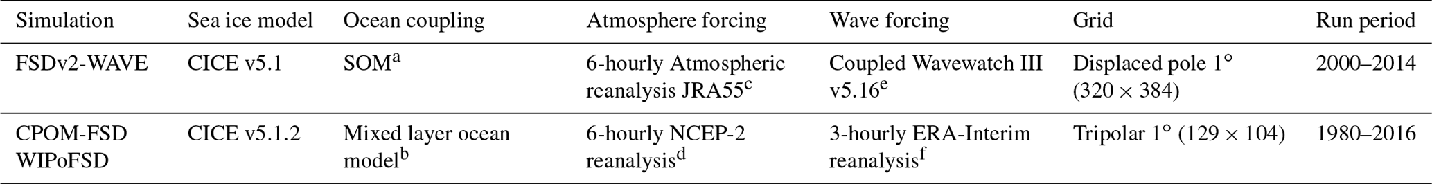
a Slab Ocean Model (SOM) (Bitz et al., 2012). b Petty et al. (2014). c Japan Meteorological Agency (2013). d Kanamitsu et al. (2002). e WAVEWATCH III Development Group (2016). f Dee et al. (2011)
3.2.1 FSDv2-WAVE model
The FSDv2-WAVE model is based on a sub-grid-scale floe size and thickness distribution (FSTD) model by Horvat and Tziperman (2015, 2017). It uses the Los Alamos Sea Ice model CICE version 5.1 (Hunke et al., 2015) and is an upgraded version of FSDv2 by coupling with a wave model. Roach et al. (2018a) further implemented this FSTD model into a global ocean–sea-ice model on the displaced gx1v6 grid (320 × 384 for a horizontal grid), which is approximately 1∘ resolution horizontally. This is the first global model that simulates emergent floe size evolution by physical processes, including lateral melt, growth, new ice formation, floe welding, and wave-induced fracture. FSDv2-WAVE uses the slab ocean model (SOM) (Bitz et al., 2012) coupled with the global ocean surface wave model Wavewatch III v5.16 (WAVEWATCH III Development Group, 2016) and incorporates a new wave-dependent ice production scheme (Roach et al., 2019). Attenuation of wave energy in the MIZ is modelled using multiple wave scattering theory developed by Meylan et al. (2021), which accounts for the sea ice floe size, sea ice thickness and sea ice concentration. To address the deficiency of the attenuation of waves when wavelengths are much greater than floe sizes in this theory, an additional attenuation scheme is applied as the reciprocal of the wave period squared in FSDv2-WAVE. Among the three selected models, FSDv2-WAVE is the only one that has a fully coupled ocean surface wave model to improve the modelling of wave attenuation, wave–ice interactions, and the associated ice thermodynamic and dynamic processes in the MIZ (Roach et al., 2019).
3.2.2 CPOM-FSD model
The CPOM-FSD model is initiated with the ice-free Arctic and run with the tripolar 1∘ (129 × 104) grids for 37 years from 1 January 1980, including a 10-year period spin-up during 1980–1989 in a pan-Arctic domain excluding Hudson Bay and the Canadian Arctic Archipelago. CPOM-FSD is adapted from the global FSTD model developed by Roach et al. (2018a, 2019) and built on a modified version of CICE v5.1.2 for sea ice simulation (hereafter referred to as CPOM-CICE) (Hunke et al., 2015; Bateson et al., 2022). CPOM-CICE is an updated version by CPOM at the University of Reading to include (i) a modified prognostic mixed-layer ocean model to better capture sea-ice–ocean feedbacks resulting from lateral and basal melt rate (Petty et al., 2014; Bateson et al., 2022), (ii) a form drag scheme for a better simulation of turbulent heat and momentum fluxes between the sea ice, ocean and atmosphere interface and representing the FSD effects on the form drag scheme (Tsamados et al., 2014; Bateson et al., 2022), and (iii) further amendments to alter maximum meltwater and snow erosion and add the “bubbly” conductivity formulation (Pringle et al., 2007; Schröder et al., 2019). A description of detailed differences between CPOM-CICE and standard CICE is available in Bateson et al. (2022). CPOM-FSD is not coupled with a wave model but instead retains the internal wave scheme from Roach et al. (2018a) and uses 3-hourly ERA-Interim reanalysis as ocean surface wave forcing. CPOM-FSD incorporates the in-plane brittle fracture and the associated FSD processes, which was shown to improve model performance in simulating the FSD (Bateson et al., 2022).
3.2.3 WIPoFSD model
WIPoFSD is a diagnostic power-law FSD model within CPOM-CICE (Bateson et al., 2020, 2022) and has the same horizontal grid, spin-up and run period as CPOM-FSD. The WIPoFSD model implements the wave-in-ice model (WIM), originally based on the ice–wave interaction theory described by Williams et al. (2013a, b) and updated to coupled ocean-waves-in-ice model NEMO–CICE–WIM at the National Oceanography Centre (NOC), UK (Hosekova et al., 2015; Rynders, 2017; Aksenov et al., 2022). Unlike the two prognostic models (FSDv2-WAVE and CPOM-FSD), the WIPoFSD model simulates an FSD following a power law with a fixed exponent of α=2.56 to constrain the FSD shape over a variable range of floe sizes. The fixed power-law exponent is determined from the satellite imagery data in Bateson et al. (2022), which is derived from MEDEA images acquired at three locations: the Chukchi Sea (70∘ N, 170∘ W), the East Siberian Sea (82∘ N, 150∘ E) and the Fram Strait (84.9∘ N, 0.5∘ E). Bateson et al. (2022) applied a power-law fit for the floe size in each image first and then calculated the averaged power-law exponent in each location. The fixed power-law exponent α=2.56 is the mean of these three locations. There are three differences between the MEDEA imagery data used by Bateson et al. (2022) for calculating the power-law exponent (hereafter Obs1) and in this study for model evaluation (hereafter Obs2). (1) The image resolution of the satellite data used for deriving Obs1 was reduced to 2 m, while the original image resolution (1 m) was kept for Obs2. (2) Obs1 was derived from three sites: the Chukchi Sea, the East Siberian Sea and the Fram Strait. Obs2 was derived from two sites (the Chukchi Sea and the Fram Strait). (3) The Obs1 datasets include 14 cases in the Chukchi Sea, 9 cases in the East Siberian Sea and 12 cases in the Fram Strait. The Obs2 datasets however include 24 cases in the Chukchi Sea and 32 cases in the Fram Strait. In addition to the exponent, the model also simulates the FSD evolution through the floe size parameter rvar, varying between minimum floe radius rmin and the maximum floe radius rmax in the distribution. rvar evolves according to four FSD processes: lateral melt, wave-induced fracture, floe growth in winter and ice advection (Bateson et al., 2020, 2022). The full details of rvar, including a physical interpretation of this value, are provided in Bateson et al. (2020).
3.3 FSD definition and evaluation metrics
In this study, the floe effective radius is used to define floe size, which is the radius of a circle that has the same area, a, as a floe. The FSD is usually defined as the fractional-area distribution, f(r)dr, and number-density distribution, n(r)dr (Rothrock and Thorndike, 1984; Toyota et al., 2006; Perovich and Jones, 2014; Horvat and Tziperman, 2015; Zhang et al., 2015; Hwang et al., 2017b; Bateson et al., 2020), corresponding to the area and the number of floes per unit ocean surface area with a radius between r and r+dr. For the evaluation of FSD models, we consider the perimeter density distribution, p(r)dr (units: km km−2), which is proportional to r⋅n(r)dr. Perimeter density distribution is defined here as the perimeter of floes per unit ice area with a radius between r and r+dr. The integral of p(r) between rmin and rmax in a radius is defined as total perimeter density:
which is the perimeter per unit ice area of floes between rmin and rmax. Roach et al. (2019) suggested that P is more related to the thermodynamic processes of sea ice floes, which is an important metric in evaluating an FSD model. Additionally, the concept of a perimeter density to characterise the overall floe size has been used in several previous observational studies (e.g. Perovich, 2002; Arntsen et al., 2015) because P reduces the impacts of partially captured floes at the edge of the image for the FSD retrieval (Perovich, 2002; Perovich and Jones, 2014). In this study, P (units: km km−2) is used to present comparisons between observations and models. Whilst information about FSD shape is lost when calculating P, we also apply p(r) (units: km km−2 km−1) to evaluate the model performance (e.g. Fig. 2), which can refer to the full perimeter density distribution. There are different ways to calculate P. In the following, we describe how the FSD models calculate P, as well as how P can be calculated from the observational FSD data, which also show the relationships between number/areal FSD and P.
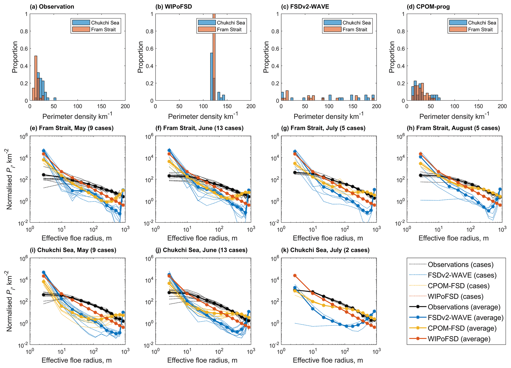
Figure 2Frequency histograms of floe P from (a) observation, (b) WIPoFSD, (c) FSDv2-WAVE and (d) CPOM-FSD. In (a)–(d), blue colour indicates the frequency distribution of P for the Chukchi Sea, and red colour is used for the Fram Strait. The p(r) value is shown for (e) May, (f) June, (g) July and (h) August in the Fram Strait as well as for (i) May, (j) June and (k) July in the Chukchi Sea. In (e)–(k), the observations are shown as a black line and the three models in different colours (FSDv2-WAVE – blue; CPOM-FSD – yellow; WIPoFSD – red). In (e)–(k), dash lines correspond to the frequency distribution of P of individual cases in each month and solid lines are their mean.
In prognostic FSD models, P is calculated from the areal FSD fi distributed into floe size categories i as follows:
where ri and wi are the midpoint and the bin width respectively for each floe size category i. Here cice represents the area-weighted SIC in the selected region and γ is a floe shape parameter, the ratio of floe perimeter to twice the floe effective radius. For example, γ=π is for circular floes. From the analysis of MEDEA-derived FSD results, the mean floe shape parameter γ is 3.60 in the Chukchi Sea region and 3.69 in the Fram Strait region, which will be used for the calculation of P in this study. Due to the limitation of image resolution in capturing the shapes of small floes, the floes of d<5 m are discarded for calculating γ.
P for WIPoFSD can be calculated from
In this equation, the power-law exponent was set as a constant, α=2.56, for WIPoFSD.
In this study, we used daily outputs from the FSD models to calculate P. To obtain P from the daily model outputs, we calculated an area-weighted mean, on the same date as the observations, over the grid cells within the study areas of the Chukchi Sea and the Fram Strait (Fig. 1). In the Supplement, we note that P varies depending on the choice of binning and calculation methods (see Sect. S2 and Fig. S1 in the Supplement). To ensure matching with the model outputs, the FSD observation data were binned into the same 12 Gaussian spacing floe size categories used by the FSD models and estimated from the areal FSD:
Aice is the total area of sea ice within the image. More details on the calculation of P is provided in the Supplement (Sect. S1).
4.1 Model evaluation: perimeter density
The comparison of P between observations and models is shown in Fig. 2. Observations show a substantial difference in P between the two regions (t test, t (47) = 6.12; p<0.001) (Fig. 2a). They showed a significantly higher P of 23.76 ± 7.53 km km−2 at the Chukchi Sea site than the P of 14.28 ± 4.45 km km−2 at the Fram Strait site (Fig. 2a). Higher P in the Chukchi Sea indicates a larger fraction of small floes in that region. It should be noted that the P values in this study are higher than the reported values from previous observational studies, which range between 5.26 and 13.68 km km−2 from May to July in the Beaufort Sea and the Chukchi Sea (Perovich, 2002; Perovich and Jones, 2014; Arntsen et al., 2015). FSDv2-WAVE P values spread out over a wide range and show the opposite regional difference to the observations (a higher P 178.37 ± 89.28 km km−2 in the Fram Strait region than the value 136.95 ± 70.58 km km−2 in the Chukchi Sea region) (Fig. 2c). WIPoFSD (Chukchi Sea: 120.93 ± 1.66 km km−2; the Fram Strait: 138.99 ± 12.98 km km−2) and CPOM-FSD (Chukchi Sea: 59.55 ± 19.13 km km−2; the Fram Strait: 61.19 ± 29.95 km km−2) also show a general overestimation of P compared to the observations and the opposite regional difference (Fig. 2b and d).
Figure 2e–k show the comparison of p(r), i.e. the perimeter of floes per unit sea ice area per unit bin width. The observation results show a declining p(r) with increasing floe radius r. The FSDv2-WAVE results show the same relationship but with a steeper slope than the observation, showing a much larger value of p(r) for small floes (r<10–30 m) whilst showing a much smaller value of p(r) for large floes (30–50 m <r<400–800) than the observations (Fig. 2e–k). This pattern is consistent in different months and regions. The CPOM-FSD results also show a similar pattern, yet the model p(r) values are in a much better agreement with the observations for large floes (r>O (10) m), especially during July and August in the Fram Strait region (Fig. 2g and h). This better match for larger floes has been shown to be due to the effects of in-plane brittle fracture (Bateson et al., 2022). The results from the two prognostic models (FSDv2-WAVE and CPOM-FSD) consistently show an “uptick” (a steepening upward slope in the largest floe size categories) in p(r) (Fig. 2e–k). This type of uptick in the prognostic models has been reported by Bateson et al. (2022) and Roach et al. (2018a) and is an artificial feature derived from the model setup of an upper floe size limit and an incomplete representation of fragmentation processes in the prognostic model for large floes. The WIPoFSD results also show a steeper slope than the observation but a better agreement with the observations than the two other model results. Similar to the two other models, the WIPoFSD model also shows an overestimation of p(r) in small floes (r<10–30 m) (Fig. 2e–k).
Now we examine the relationship between SIC and P. The observation results show a negative relationship between SIC and P (correlation coefficient ; p<0.01), which means higher P in a lower SIC (i.e. the presence of smaller floes in a lower SIC). A similar relationship was found by Perovich (2002) and Perovich and Jones (2014) in July to September. The WIPoFSD model shows the same negative relationship between SIC and P with stronger correlation (, p<0.01), but overall P values are much larger than the observations (Fig. 3). In the Chukchi region, the P values are mostly located within the “pack ice” region (SIC >80 %) for both the observations and WIPoFSD model outputs (Fig. 3a). In the Fram Strait, however, the WIPoFSD P values are shifted toward a lower SIC than the observations (Fig. 3b).
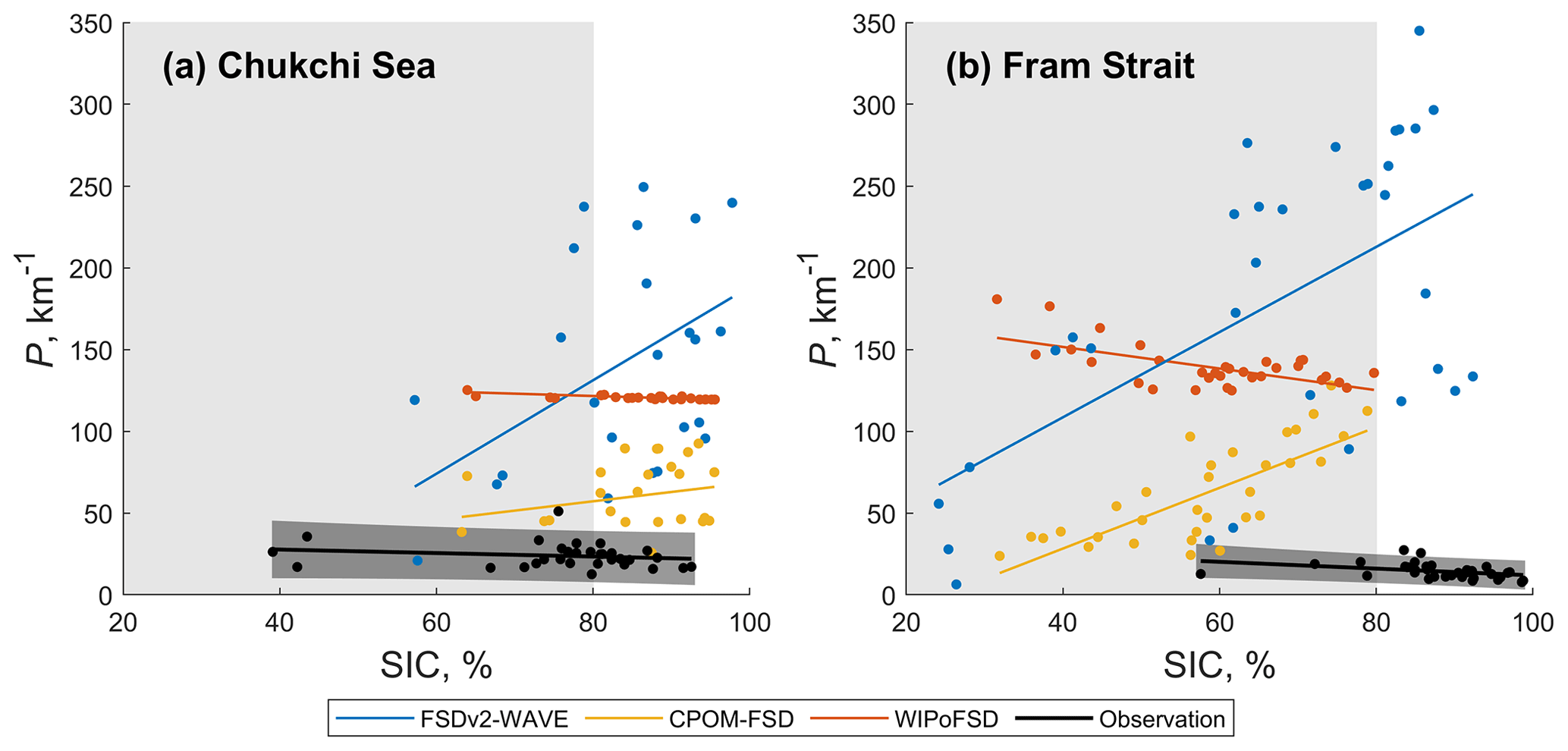
Figure 3Perimeter density P according to SIC for (a) the Chukchi Sea region and (b) the Fram Strait region. Dark grey shades along the regression lines of the observations mark a 95 % confidence interval. The light grey shade marks the MIZ, defined as SIC between 15 % and 80 %.
The two prognostic models show an opposite correlation to the observations and WIPoFSD results. Both FSDv2-WAVE and CPOM-FSD data show positive relationships between SIC and P (rcor=0.35 and 0.38, p<0.01) (Fig. 3). In the pack ice region (SIC >80 %), the two prognostic models simulate much higher P than the observations; in particular the P values from FSDv2-WAVE are almost 7–16 times higher than the observations in both study regions (Fig. 3). This indicates a much higher floe fragmentation in the model simulations than the observations under pack ice conditions. At a low ice concentration, the difference becomes smaller, especially for CPOM-FSD (Fig. 3).
4.2 Effects of image resolution on the FSD retrieval
In Sect. 4.1, the three models all show a larger value of p(r) for small floes (r<10–30 m) than the observations (Fig. 2e–k). The limited image resolution may hinder the retrieval of small floes. To test this, we investigate p(r) derived from MEDEA (δ=1 m) images and from WV (δ=0.5 m) images (Fig. 4). The results show that the p(r) values from the images are in a good agreement for the floes with r>∼15 m (Fig. 4e and f). This confirms the compatibility of the FSD retrieval from the images with different resolutions. Importantly, however, for the floes with a floe radius r smaller than ∼ 15 m, p(r) derived from the WV image becomes significantly higher than the MEDEA-derived p(r) values (Fig. 4e and f). The difference in the p(r) integrated in the two smallest bins (r<14.29 m) between the WV and MEDEA images reaches 1.12 km km−2 (Fig. 4e) in the cases in Fig. 4a and b and 3.48 km km−2 (Fig. 4f) in the cases in Fig. 4c and d.
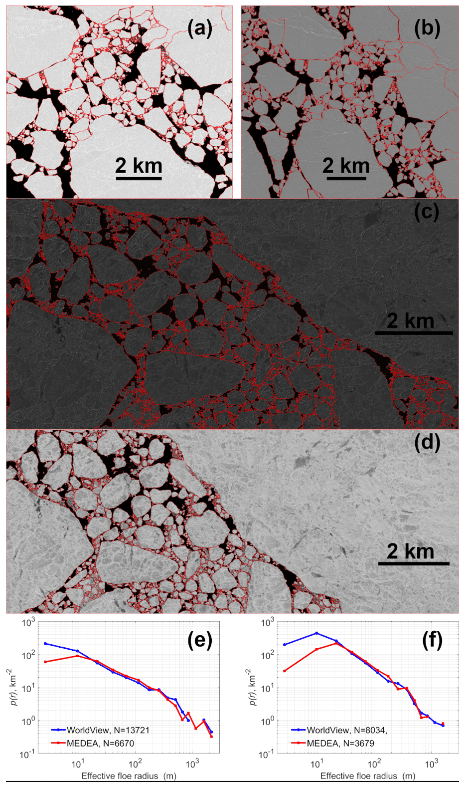
Figure 4Comparison of perimeter density distribution p(r) between (a) WV© image (δ=0.5 m) and (b) MEDEA image (δ=1 m) on 5 June 2013 at 84.9∘ N, 0.1∘ E (Fram Strait) is shown in (e) and between (c) WV image (δ=0.5 m) on 1 June 2013 and (d) MEDEA image (δ=1 m) on 31 May 2013 at 70∘ N, 170∘ W (Chukchi Sea) is shown in (f). The image size of the co-located scenes shown in (a), (b), (c) and (d) cover an area of 106, 82, 66 and 64 km2 respectively. In panels (e)–(f), N is the number of floes derived from satellite images.
4.3 Model evaluation: sea ice concentration
The FSD models considered in this study include parameterisations with dependencies on SIC. For example, the floe welding rate is set to be proportional to the square of SIC in the two prognostic models – FSDv2-WAVE and CPOM-FSD – based on the work of Roach et al. (2018b). It is therefore useful to evaluate how well the models simulate the observed SIC and consider the extent to which errors in the simulated SIC could explain the differences between models and observations in simulating floe perimeter density. In the Chukchi Sea, CPOM-FSD shows a good agreement in SIC with the observations (correlation coefficient rcor>0.98; RMSE <7 %) (Table 2). FSDv2-WAVE, however, shows a considerable bias, underestimating SIC by 16 %–17 % compared to the observations (Fig. 5a). In the Fram Strait, FSDv2-WAVE agrees better with the observations (rcor>0.90; RMSE <7 %; Table 2) than with CPOM-FSD (Fig. 5b). For example, the RMSEs for CPOM-FSD are more than 2 times larger than FSDv2-WAVE (Table 2). FSDv2-WAVE slightly underestimates SIC by 2 %–4 % compared to the observations in the MIZ (SIC <80 %). CPOM-FSD strongly underestimate the SIC by 13 %–15 % in the MIZ compared to the observations.
Table 2Statistical summary for the two prognostic FSD models against the NSIDC SIC and ASI SIC. NSIDC and ASI SIC data used for the comparison are from between April and August for the analysis period of 2000–2014.
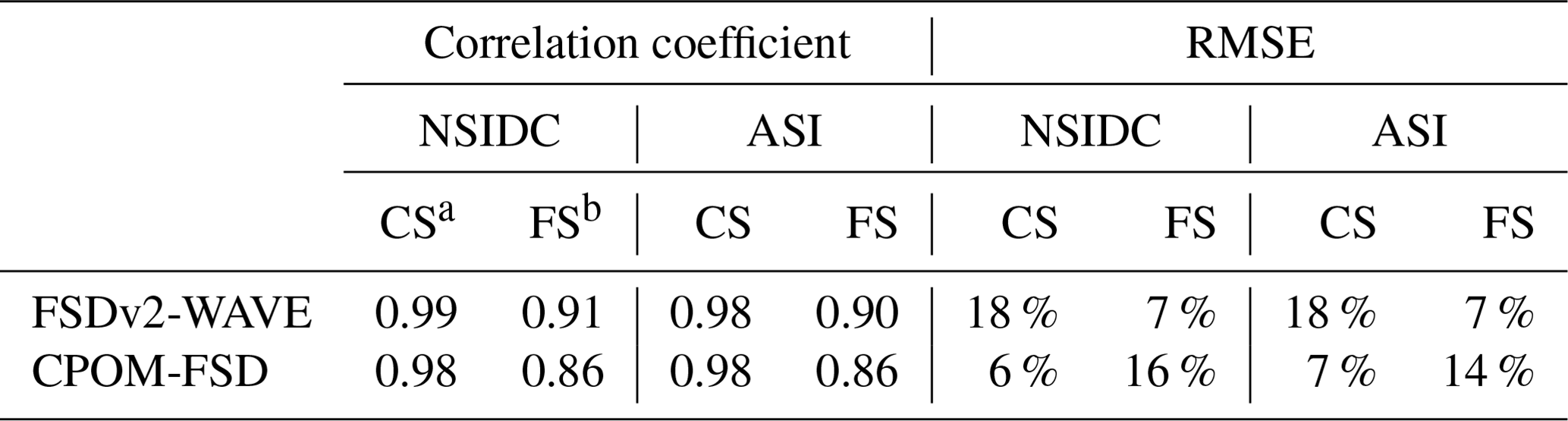
a Chukchi Sea. b Fram Strait.
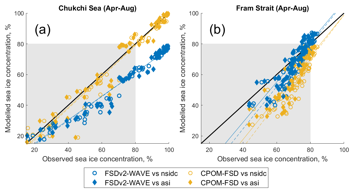
Figure 5A comparison of SIC between observations and prognostic models in the Chukchi Sea (a) and the Fram Strait (b). Monthly SIC data from April to August for the period 2000–2014 were used for the comparison. In (a)–(b), the comparison between the observations and two prognostic models is shown in different colours (FSDv2WAVE: blue; CPOM-FSD: yellow). The comparison between NSIDC and models are marked with circles and their linear fits are shown as a dashed line. Diamonds and solid lines indicate the comparison between ASI and models.
This difference in SIC between FSDv2-WAVE and CPOM-FSD can be attributed to different atmospheric forcing that is used in the models (Schröder et al., 2019). FSDv2-WAVE uses JRA55b reanalysis data for the atmospheric forcing, whilst CPOM-FSD and WIPoFSD use 6-hourly NCEP-2 reanalysis data (Table 1). The underestimated SIC from the two prognostic models will result in too small a floe welding rate during spring and early summer. A negative bias in spring SIC shown in the prognostic models may partially explain the overestimation of P and in particular the overestimation of p(r) for small floes and the underestimation of p(r) for large floes (Fig. 2).
For the WIPoFSD model, the evolution of P is constrained by the floe size parameter rvar (Eq. 3), which is also impacted by a simple floe growth restoration scheme including floe welding, lateral growth and new ice formation (Bateson et al., 2020). However, this floe growth restoration scheme is not closely related to SIC. In contrast to the other schemes, changes in rvar are linked to SIC in the WIPoFSD model via lateral melt, which acts to reduce both (Bateson et al., 2020, 2022). For WIPoFSD, SIC decreases by 40 % in the Chukchi Sea from May to July, similar to the observed decrease (39 %) from NSIDC SIC and ASI SIC. In contrast, the SIC for WIPoFSD decreased by about 20 % in the Fram Strait, 2 times more than in the observations (9 %). Bateson et al. (2020) conducted a sensitivity study to test the role of lateral melting in affecting the FSD by removing the lateral melt feedback on floe size. The results demonstrate that lateral melt is less important in changing the FSD in WIPoFSD. This could explain a smaller-discrepancy P between the WIPoFSD model and the observations than between the other two models (Fig. 2).
4.4 Processes controlling floe size distribution evolution
In the prognostic models, the FSD evolution is constrained by the parameterised processes. In the period of May–August, the dominant FSD evolution processes are lateral melt and wave-induced breakup, as lateral growth, new ice formation and floe welding are negligible during this season. To test the effects of lateral melt and wave breakup, we acquired two datasets from model outputs (Fig. 6): monthly changes in P arising from lateral melt and the FSD changes arising from wave breakup. The results show that FSDv2-WAVE produces larger, positive changes in P from wave fracture (Fig. 6b and d) in summer relative to CPOM-FSD (Fig. 6f and h). This indicates that the wave-induced fracture process is much more significant for the floe fragmentation in FSDv2-WAVE than in CPOM-FSD. The more significant wave breakup in FSDv2-WAVE may be attributed to the fact that FSDv2-WAVE uses a coupled ocean wave scheme rather than an in-ice wave scheme used in the CPOM-FSD model and that the SIC in the Chukchi Sea is significantly lower in FSDv2-WAVE, which is forced with the JRA55a reanalysis, while CPOM-FSD are forced with the NCEP-2 reanalysis.
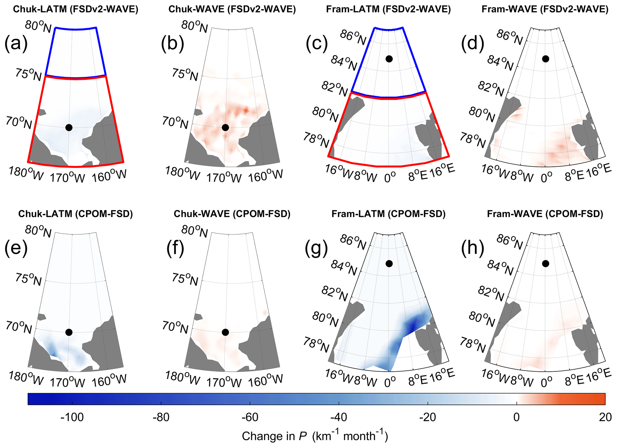
Figure 6Monthly changes in P simulated by the two prognostic models over the period May to July during 2000–2014. (a) Change in P arising from lateral melt for FSDv2-WAVE in the Chukchi Sea. Panel (b) is the same as (a) but for wave-induced P change. Panels (c) and (d) are the same as (a) and (b) but in the Fram Strait. Panels (e)–(h) are the same as (a)–(d) but for CPOM-FSD. The blue and red outlines in (a) and (c) show the northern and southern region of the two study regions. Black dots indicate the location of observations in the study regions.
CPOM-FSD shows a stronger reduction in P arising from lateral melt (Fig. 6e and g) in summer than FSDv2-WAVE. This indicates that the lateral melt process is much more dominant in CPOM-FSD than FSDv2-WAVE. The difference in lateral melt is likely to be related to the difference in sea surface temperature in the models. CPOM-FSD uses a prognostic mixed-layer ocean model and a form drag scheme to simulate ocean mixed-layer properties and the impact of topography of sea ice on sea-ice–ocean–atmosphere heat exchange (Bateson et al., 2022). On the other hand, FSDv2-WAVE uses a single ocean layer and ocean heat content diagnosed from a run of Community Climate System Model version 4 (Roach et al., 2019). This difference in ocean components can produce different oceanic heat fluxes in determining the strength of lateral melt between FSDv2-WAVE and CPOM-FSD.
In the northern Chukchi Sea and the Fram Strait (blue outlines in Fig. 6), the change in P arising from processes driving FSD change during May–August is almost zero in the two prognostic models. The P in the northern regions can be regarded as a fixed value over the period of May–August. Our FSD observations lie in the southern part (red outline in Fig. 6a) of the Chukchi Sea region, where both models show large changes in P due to wave fracture and lateral melt compared with the northern Chukchi Sea region (blue outline in Fig. 6a). For the Fram Strait region, the observation site is located in the northern region where sea ice floes experience weaker lateral melt and wave fracture (blue outline in Fig. 6c). To test the sensitivity of model P between the northern (weak wave fracture and lateral melt) and southern (strong wave fracture and lateral melt) regions, we calculated and compared P from both models between the southern and northern regions of the Chukchi Sea and the Fram Strait. The purpose of this comparison is to explore whether the differences between observations and models arise from the inaccurate summer FSD evolution processes simulated by models (lateral melt and wave fracture) or the processes that determine FSD shape prior to summer breakup.
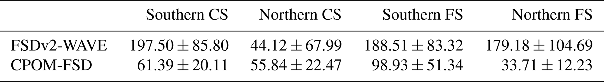
As expected, the results show a considerable difference in P between the two regions (Fig. 7). The P values from the northern regions are smaller than the values from the southern regions for the two models (Fig. 7). In the Chukchi Sea region, the SIC values from the northern region are clustered between 90 % and 100%, and the P values for both models are comparable to the observation values (Fig. 7a). In the Fram Strait, the SIC values from the northern region spread over a wider range of 50 %–100 % (Fig. 7b). Interestingly, CPOM-FSD results from the northern Fram Strait region become very comparable to the observations in terms of the P values and the range of SIC (Fig. 7a), while the P values from FSDv2-WAVE still show much larger values (Fig. 7b and Table 3). Note that the observation site in the Fram Strait is located within the northern region. In a direct comparison encompassing a larger model region (Fig. 3), the P values from CPOM-FSD were larger than the observation values (and there is a positive correlation with SIC). The P in the northern Fram Strait simulated by CPOM-FSD is of the same order of magnitude as the observations, indicating a closer match between CPOM-FSD and the observations in the northern Fram Strait region than in the southern region. This suggests that no significant wave fracture and lateral melt has occurred at the observation site. This can be supported by the fact that most of the satellite observations in the Fram Strait represent regions where the sea ice has experienced fewer thermodynamic and dynamic impacts (e.g. Fig. 1c), so the effects of lateral melt and wave fracture were likely small. It should be noted that CPOM-FSD implements in-plane brittle fracture in the model. Recent studies suggest that brittle fracture can determine the initial FSD in spring before wave fracture and lateral melt (Gherardi and Lagomarsino, 2015). Therefore, the close agreement between CPOM-FSD and the observations may represent the initial state of the FSD before any significant wave fracture and lateral melt occur. In the case of FSDv2-WAVE, the P values from the northern Fram Strait region still show much larger numbers. It is difficult to pinpoint the exact causes of this overestimation as the effects of wave fracture would be quite small in the northern region (Fig. 6d).
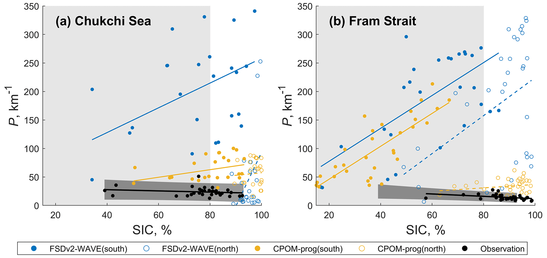
Figure 7Similar to Fig. 3 but showing the comparison between observations (black) and two prognostic models (FSDv2-WAVE – blue; CPOM-FSD – yellow) in southern regions (solid circle) and northern regions (hollow circle) of the study region in the Chukchi Sea (a) and the Fram Strait (b).
Table 3The mean P (km km−2) and standard deviation simulated by FSDv2-WAVE and CPOM-FSD in the southern regions and northern regions of the Chukchi Sea (CS) region and the Fram Strait (FS) region.
In this study, we evaluate three state-of-art FSD models (FSDv2-WAVE, CPOM-FSD and WIPoFSD) against new observation data derived from 1 m resolution MEDEA imagery. The observation results show clear regional differences between the two study regions, i.e. much larger perimeter density P in the Chukchi Sea region than in the Fram Strait region. Model outputs, however, fail to show such a regional difference.
The direct comparison between the observations and daily model outputs reveals that the models consistently show (i) overall overestimation of P, (ii) much larger values of the p(r) for small floes (r<10–30 m) and (iii) much smaller values of the p(r) for the larger floes (30–50 m <r<400–800 m). Among the three FSD models, WIPoFSD and CPOM-FSD show a much smaller difference to the observations than FSDv2-WAVE. The observations and the WIPoFSD model both show a negative correlation between SIC and P (i.e. smaller floes in a lower SIC), while the two prognostic models show the opposite (positive) correlation. The causes of such differences include (i) differences in the coverage area of study regions between models and observations, (ii) the limitations within the observations such as the image resolution, (iii) underestimation of SIC and the associated effects on floe welding parameterisation, and (iv) too much wave fragmentation in the models, as suggested by Cooper et al. (2022).
The satellite observation sites are fixed and much smaller than the regions selected for models, which include grid cells in both MIZ and interior pack ice. Nevertheless, the observations also include a range of different sea ice conditions. For example, the sea ice concentration of half of the cases in the Chukchi Sea (Fig. 2i–k) is below 80 %, indicating almost half of the images within the MIZ and the other half within the interior ice pack. Therefore, the monthly means from the models (solid lines in Fig. 2e–k) can be comparable to the observations in the Chukchi Sea. In the Fram Strait, most of the observations represent the pack ice (>80 % SIC), while the model outputs mainly represent the MIZ conditions (<80 % SIC). To evaluate the effects of the size of modelling study regions, we reduced the size of the model domains down to a five by five grid cell region at the centre of the observation sites, which shows the same overestimation of P and p(r) of small floes (see Fig. S2 and Table S3). Based on this evaluation, we decided to use a larger model domain to better capture spatial variability caused by different external forcing fields in the models.
The effects of the limited image resolution are examined by comparing (1 m resolution) MEDEA-derived p(r) with (∼ 0.5 m resolution) WV-derived p(r). It shows that WV-derived p(r) integrated for the two smallest bins (r<14.29 m) is 1.12 to 3.48 km km−2 larger than the value derived from MEDEA. However, this difference is still too small to explain the difference between the observations and model outputs, varying between 20.42 and 218.95 km km−2 in Fig. 2e–k (See Table S1). We do not know how much additional change we would see in P and p(r) if we had access to imagery at even higher resolutions. This suggests that based on the recent satellite imagery, the image resolution could be one of the contributors but is not the main contributor to the overestimation of modelled p of small floes. It is also worth noting that both 1 and 0.5 m resolution observations show two distinct regimes of p for small floes (r<O (10) m) and the larger floes (Figs. 2e–k, 4e and f). This situation is associated with several possible reasons: (i) image resolution is not high enough to identify all small floes accurately; (ii) lateral melt reduced the number of small floes (Hwang and Wang, 2022); and (iii) other statistical models, e.g. log-normal distribution, are better to describe the FSDs rather than power laws (Montiel and Mokus, 2022; Mokus and Montiel, 2022). It requires much higher-resolution images (e.g. aerial photographs) and further research in the future to properly investigate the effects of the image resolution and the reasons of this deviation of the small floe perimeter density distribution.
The strength of floe welding is strongly contributed from the SIC in the prognostic models evaluated in this study (Roach et al., 2018a, b; Bateson, 2021a; Bateson et al., 2022). Previous studies have identified the dominant role of floe welding in the formation processes of large floes (Toyota et al., 2011; Roach et al., 2018a, b). In particular, Bateson (2021a) has assessed the effects of floe welding on the p(r) in the CPOM-FSD model, suggesting that floe welding occurring in spring can influence the FSD in summer. A low ice concentration reduces the floe welding during spring and consequently results in an initial over-fragmented state in early summer. Therefore, a negative bias in spring SIC shown in the prognostic models can partially explain the overestimation of p(r) for small floes and the underestimation of p(r) for larger floes in the two prognostic models (Fig. 2).
For WIPoFSD, the bias in p(r) is not related to the underestimation of SIC and the consequent floe welding parameterisation. Instead, the bias in p(r) is likely due to the fixed power-law exponent of α=2.56 for the non-cumulative distribution used in the model. This value is larger than the exponent from our dataset (i.e. in the Chukchi Sea α=2.34; in the Fram Strait α=2.07). Previous studies have found that the exponent ranges vary seasonally and regionally (Stern et al., 2018a, b). The typical exponent value ranges from about 1.8 to 3.6 for non-cumulative distribution in the Chukchi Sea and the Beaufort Sea during May–August (Holt and Martin, 2001; Wang et al., 2016; Hwang et al., 2017b; Stern et al., 2018a, b) and from 2.0 to 2.8 (non-cumulative distribution) in the Fram Strait in June (Kergomard, 1989). Thus, we suggest that employing a seasonally and spatially variable exponent in the model may improve the model performance.
In terms of overactive wave fracture in the prognostic models, the wave fracture model applied by Horvat and Tziperman (2015) and Horvat and Roach (2022) has been implicated in producing unrealistically fragmented FSDs in the Chukchi Sea (Cooper et al., 2022). As wave events episodically propagate hundreds of kilometres into the sea ice, the impact of this oversensitivity may be to produce unrealistically high perimeter densities in our study regions. To investigate this, we examined the P in the northern regions where wave-induced breakup is negligible. In these regions, most modelled P values match our observations better. However, we found that the P from FSDv2-WAVE still shows positive bias in the Fram Strait region. These biases may be attributed to the initially over-fragmented ice conditions in early spring set in the models.
In conclusion, the new FSD dataset was found to be valuable in evaluating the FSD models, which show considerable differences from the observations in terms of P and the relationship between P and SIC. The summer P change in the models depends strongly on initial floe size distribution before melting starts, which is affected by floe formation and growth processes (e.g. the welding of metre-scale floes) in the models. Our findings also indicate that positive biases of P are closely linked to overactive wave fracture in the models. This suggests that accurate parameterisation of wave-induced sea ice breakup is essential for simulating the summer FSD correctly. It should be noted that both the prognostic FSD model and power-law FSD model are still in development, as are methodologies to determine floe size from satellite imagery. In addition, the ability to resolve the shape of the FSD for small floes remains constrained by the limited resolution of satellite images. Nevertheless, this study shows how model evaluation using such imagery can be used to produce key insights for model development, thus allowing us to improve sea ice model performance for climate research and operational applications.
MEDEA images are openly available at the Global Fiducials Library website (https://www.usgs.gov/global-fiducials-library-data-access-portal, United States Geological Survey, 2023). WorldView images cannot be shared due to the license. However, the images can be ordered from LAND INFO Satellite Imagery Search Portal (2023, https://search.landinfo.com/) or other satellite imagery providers. FSD imagery data retrieved from satellite imagery in this study can be accessible from UK Polar Data Centre (https://doi.org/10.5285/6d65b406-237c-425d-9356-39b77ac30e85, Hwang and Wang, 2023). The model outputs used for analysing the monthly change of FSD in the study are available from https://doi.org/10.5281/zenodo.3463580 (Roach, 2019) for FSDv2-WAVE (Roach et al., 2019) and from https://doi.org/10.17864/1947.300 for CPOM-FSD and WIPoFSD (Bateson et al., 2021b). The daily model outputs used in this study for model-observation comparison is provided in the Supplement.
The supplement related to this article is available online at: https://doi.org/10.5194/tc-17-3575-2023-supplement.
YW conceived the study under the supervision of BH, YA and CH. YW prepared the FSD observations with the support from BH. AWB completed simulations of CPOM-FSD and WIPoFSD and shared model outputs from Bateson et al. (2022). YW performed the data analysis and completed the comparison of the FSD observations to model output, with support from BH, AWB, YA and CH. YW prepared the paper with guidance and contributions from all authors.
At least one of the (co-)authors is a member of the editorial board of The Cryosphere. The peer-review process was guided by an independent editor, and the authors also have no other competing interests to declare.
Publisher’s note: Copernicus Publications remains neutral with regard to jurisdictional claims in published maps and institutional affiliations.
Initial FSD model development for WIPoFSD model used in this study first has been implemented in the NEMO–CICE–WIM sea ice–ocean–waves interaction model by Lucia Hosekova, Stefanie Rynders and Yevgeny Aksenov at the National Oceanography Centre (NOC) under the EC FP7 project “Ships and Waves Reaching Polar Regions” (SWARP) in 2014–2017 (https://cordis.europa.eu/project/id/607476, last access: 15 August 2023, grant agreement 607476). Details of the model development are described by Rynders (2017) and Bateson et al. (2022). We are grateful to Lettie Roach for providing daily model outputs from the FSDv2-WAVE model described by Roach et al. (2019). We thank the editor Stephen Howell, referee Fabien Montiel and one anonymous referee for their constructive comments.
This research is supported by the UK Natural Environment Research Council (NERC) under the project Toward a Marginal Arctic Sea Ice (grant no. NE/R000654/1) and the project Arctic Sea Ice Breakup and Floe Size during the Autumn-to-Summer Transition (MOSAiCFSD) (grant no. NE/S002545/1) for Yanan Wang and Byongjun Hwang. Adam Bateson was supported by NERC (grant nos. NE/R016690/ and NE/R000654/1). Yevgeny Aksenov acknowledges financial support from NERC grant nos. NE/R000085/1 and NE/R000085/2 (Toward a Marginal Arctic Sea Ice), NE/T000260/1 (PRE-MELT: Preconditioning the trigger for rapid Arctic ice melt) and NE/N018044/1 (the North Atlantic Climate System Integrated Study LTSM Programme ACSIS) and from the NERC National Capability CLASS (Climate Linked Atlantic Sector Science LTS-S Programme), grant no. NE/R015953/1. Christopher Horvat was supported by NASA (grant no. 80NSSC20K0959) and through the Scale Aware Sea Ice Project (SASIP). SASIP is supported by Schmidt Futures, a philanthropic initiative that seeks to improve societal outcomes through the development of emerging science and technologies.
This paper was edited by Stephen Howell and reviewed by Fabien Montiel and one anonymous referee.
Aksenov, Y., Popova, E. E., Yool, A., Nurser, A. J. G., Williams, T. D., Bertino, L., and Bergh, J.: On the future navigability of Arctic sea routes: High-resolution projections of the Arctic Ocean and sea ice, Mar. Policy, 75, 300–317, https://doi.org/10.1016/j.marpol.2015.12.027, 2017.
Aksenov, Y., Rynders, S., Feltham, D. L., Hosekova, L., Marsh, R., Skliris, N., Bertino, L., Williams, T. D., Popova, E., Yool, A., Nurser, A. J. G., Coward, A., Bricheno, L., Srokosz, M., and Heorton, H.: Safer Operations in Changing Ice-Covered Seas: Approaches and Perspectives, in: IUTAM Symposium on Physics and Mechanics of Sea Ice, edited by: Uhkuri, J. and Polojärvi, A., IUTAM Bookseries, vol 39. Springer, Cham, Espoo, Finland, 241–260, https://doi.org/10.1007/978-3-030-80439-8_12, 2022.
Arntsen, A. E., Song, A. J., Perovich, D. K., and Richter-Menge, J. A.: Observations of the summer breakup of an Arctic sea ice cover, Geophys. Res. Lett., 42, 8057–8063, https://doi.org/10.1002/2015GL065224, 2015.
Bateson, A. W.: Fragmentation and melting of the sea- sonal sea ice cover, PhD thesis, Department of Meteo- rology, University of Reading, United Kingdom, 293 pp., https://doi.org/10.48683/1926.00098821, 2021a.
Bateson, A. W.: Simulations of the Arctic sea ice comparing different approaches to modelling the floe size distribution and their respective impacts on the sea ice cover, University of Reading [data set], https://doi.org/10.17864/1947.300, 2021b.
Bateson, A. W., Feltham, D. L., Schröder, D., Hosekova, L., Ridley, J. K., and Aksenov, Y.: Impact of sea ice floe size distribution on seasonal fragmentation and melt of Arctic sea ice, The Cryosphere, 14, 403–428, https://doi.org/10.5194/tc-14-403-2020, 2020.
Bateson, A. W., Feltham, D. L., Schröder, D., Wang, Y., Hwang, B., Ridley, J. K., and Aksenov, Y.: Sea ice floe size: its impact on pan-Arctic and local ice mass and required model complexity, The Cryosphere, 16, 2565–2593, https://doi.org/10.5194/tc-16-2565-2022, 2022.
Bennetts, L. G., O'Farrell, S., and Uotila, P.: Brief communication: Impacts of ocean-wave-induced breakup of Antarctic sea ice via thermodynamics in a stand-alone version of the CICE sea-ice model, The Cryosphere, 11, 1035–1040, https://doi.org/10.5194/tc-11-1035-2017, 2017.
Birnbaum, G. and Lüpkes, C.: A new parameterization of surface drag in the marginal sea ice zone, Tellus A, 54, 107–123, https://doi.org/10.3402/tellusa.v54i1.12121, 2002.
Bitz, C. M., Shell, K. M., Gent, P. R., Bailey, D. A., Danabasoglu, G., Armour, K. C., Holland, M. M., and Kiehl, J. T.: Climate Sensitivity of the Community Climate System Model, Version 4, 25, 3053–3070, https://doi.org/10.1175/JCLI-D-11-00290.1, 2012.
Brenner, S., Rainville, L., Thomson, J., Cole, S., and Lee, C.: Comparing Observations and Parameterizations of Ice-Ocean Drag Through an Annual Cycle Across the Beaufort Sea, J. Geophys. Res.-Oceans, 126, e2020JC016977, https://doi.org/10.1029/2020JC016977, 2021.
Burroughs, S. M. and Tebbens, S. F.: Upper-truncated Power Laws in Natural Systems, Pure Appl. Geophys., 158, 741–757, https://doi.org/10.1007/PL00001202, 2001.
Cooper, V. T., Roach, L. A., Thomson, J., Brenner, S. D., Smith, M. M., Meylan, M. H., and Bitz, C. M.: Wind waves in sea ice of the western Arctic and a global coupled wave-ice model, Philos. T. R. Soc. A, 380, 20210258, https://doi.org/10.1098/rsta.2021.0258, 2022.
Dee, D. P., Uppala, S. M., Simmons, A. J., Berrisford, P., Poli, P., Kobayashi, S., Andrae, U., Balmaseda, M. A., Balsamo, G., Bauer, P., Bechtold, P., Beljaars, A. C. M., van de Berg, L., Bidlot, J., Bormann, N., Delsol, C., Dragani, R., Fuentes, M., Geer, A. J., Haimberger, L., Healy, S. B., Hersbach, H., Hólm, E. V., Isaksen, L., Kållberg, P., Köhler, M., Matricardi, M., Mcnally, A. P., Monge-Sanz, B. M., Morcrette, J. J., Park, B. K., Peubey, C., de Rosnay, P., Tavolato, C., Thépaut, J. N., and Vitart, F.: The ERA-Interim reanalysis: Configuration and performance of the data assimilation system, Q. J. Roy. Meteor. Soc., 137, 553–597, https://doi.org/10.1002/qj.828, 2011.
Denton, A. A. and Timmermans, M.-L.: Characterizing the sea-ice floe size distribution in the Canada Basin from high-resolution optical satellite imagery, The Cryosphere, 16, 1563–1578, https://doi.org/10.5194/tc-16-1563-2022, 2022.
Dumas-Lefebvre, E. and Dumont, D.: Aerial observations of sea ice breakup by ship waves, The Cryosphere, 17, 827–842, https://doi.org/10.5194/tc-17-827-2023, 2023.
Dumont, D.: Marginal ice zone dynamics: history, definitions and research perspectives, Philos. T. R. Soc. A, 380, 20210253, https://doi.org/10.1098/rsta.2021.0253, 2022.
Feltham, D. L.: Granular flow in the marginal ice zone, Philos. Trans. R. Soc. A Math. Phys. Eng. Sci., 363, 1677–1700, https://doi.org/10.1098/RSTA.2005.1601, 2005.
Gherardi, M. and Lagomarsino, M. C.: Characterizing the size and shape of sea ice floes, Sci. Rep., 5, 10226, https://doi.org/10.1038/srep10226, 2015.
Herman, A.: Sea-ice floe-size distribution in the context of spontaneous scaling emergence in stochastic systems, Phys. Rev. E, 81, 066123, https://doi.org/10.1103/PhysRevE.81.066123, 2010.
Herman, A.: Wave-induced stress and breaking of sea ice in a coupled hydrodynamic discrete-element wave–ice model, The Cryosphere, 11, 2711–2725, https://doi.org/10.5194/tc-11-2711-2017, 2017.
Herman, A., Evers, K.-U., and Reimer, N.: Floe-size distributions in laboratory ice broken by waves, The Cryosphere, 12, 685–699, https://doi.org/10.5194/tc-12-685-2018, 2018.
Herman, A., Wenta, M., and Cheng, S.: Sizes and Shapes of Sea Ice Floes Broken by Waves – A Case Study From the East Antarctic Coast, Front. Earth Sci., 9, 655977, https://doi.org/10.3389/feart.2021.655977, 2021.
Holt, B. and Martin, S.: The effect of a storm on the 1992 summer sea ice cover of the Beaufort, Chukchi, and East Siberian Seas, J. Geophys. Res.-Oceans, 106, 1017–1032, https://doi.org/10.1029/1999JC000110, 2001.
Horvat, C.: Marginal ice zone fraction benchmarks sea ice and climate model skill, Nat. Commun., 12, 2221, https://doi.org/10.1038/s41467-021-22004-7, 2021.
Horvat, C. and Roach, L. A.: WIFF1.0: a hybrid machine-learning-based parameterization of wave-induced sea ice floe fracture, Geosci. Model Dev., 15, 803–814, https://doi.org/10.5194/gmd-15-803-2022, 2022.
Horvat, C. and Tziperman, E.: A prognostic model of the sea-ice floe size and thickness distribution, The Cryosphere, 9, 2119–2134, https://doi.org/10.5194/tc-9-2119-2015, 2015.
Horvat, C. and Tziperman, E.: The evolution of scaling laws in the sea ice floe size distribution, J. Geophys. Res.-Oceans, 122, 7630–7650, https://doi.org/10.1002/2016JC012573, 2017.
Horvat, C., Tziperman, E., and Campin, J. M.: Interaction of sea ice floe size, ocean eddies, and sea ice melting, Geophys. Res. Lett., 43, 8083–8090, https://doi.org/10.1002/2016GL069742, 2016.
Horvat, C., Blanchard-Wrigglesworth, E., and Petty, A.: Observing Waves in Sea Ice With ICESat-2, Geophys. Res. Lett., 47, e2020GL087629, https://doi.org/10.1029/2020GL087629, 2020.
Hosekova, L., Aksenov, Y., Coward, A., Williams, T., Bertino, L., and Nurser, A. J. G.: Modelling Sea Ice and Surface Wave Interactions in Polar Regions, in: AGU Fall Meeting Abstracts, 15–18 December 2015, San Francisco, USA, GC34A-06, https://agu.confex.com/agu/fm15/webprogram/Paper72536.html (last access: 22 August 2023), 2015.
Hunke, E. C., Lipscomb, W. H., Turner, A. K., Jeffery, N., and Elliott, S.: CICE: the Los Alamos Sea Ice Model Documentation and Software User’s Manual Version 5.1 LA-CC-06-012, Tech. Rep., Los Alamos National Laboratory, https://svn-ccsm-models.cgd.ucar.edu/cesm1/alphas/branches/cesm1_5_alpha04c_timers/components/cice/src/doc/cicedoc.pdf (last access: 14 August 2023), 2015.
Hwang, B., Ren, J., McCormack, S., Berry, C., Ayed, I. Ben, Graber, H. C., and Aptoula, E.: A practical algorithm for the retrieval of floe size distribution of Arctic sea ice from high-resolution satellite Synthetic Aperture Radar imagery, Elem. Sci. Anthr., 5, 38, https://doi.org/10.1525/elementa.154, 2017a.
Hwang, B., Wilkinson, J., Maksym, T., Graber, H. C., Schweiger, A., Horvat, C., Perovich, D. K., Arntsen, A. E., Stanton, T. P., Ren, J., and Wadhams, P.: Winter-to-summer transition of Arctic sea ice breakup and floe size distribution in the Beaufort Sea, Elem. Sci. Anthr., 5, 40, https://doi.org/10.1525/elementa.232, 2017b.
Hwang, B. and Wang, Y.: Multi-scale satellite observation of the Arctic sea ice : a new insight into the life cycle of floe size distribution, Phil. Trans. R. Soc. A, 380, 20210259, https://doi.org/10.1098/rsta.2021.0259, 2022.
Hwang, B. and Wang, Y.: High-resolution floe size distribution of Arctic sea ice 2000–2014 (Version 1.0), NERC EDS UK Polar Data Centre [data set], https://doi.org/10.5285/6d65b406-237c-425d-9356-39b77ac30e85, 2023.
Japan Meteorological Agency: JRA-55: Japanese 55-year reanalysis, daily 3-hourly and 6-hourly data, Japan Meteorological Agency [data set], https://doi.org/10.5065/D6HH6H41, 2013.
Kanamitsu, M., Ebisuzaki, W., Woollen, J., Yang, S. K., Hnilo, J. J., Fiorino, M., and Potter, G. L.: NCEP-DOE AMIP-II reanalysis (R-2), B. Am. Meteorol. Soc., 83, 1631–1644, https://doi.org/10.1175/BAMS-83-11-1631, 2002.
Kergomard, C.: Analyse morphometrique de la zone marginale de la banquise polaire au nord-ouest du Spitsberg a partir de l'imagerie SPOT panchromatique, Bulletin-Société Française de Photogrammétrie et de Télédétection, 115, 17–19, 1989.
Kohout, A. L. and Meylan, M. H.: An elastic plate model for wave attenuation and ice floe breaking in the marginal ice zone, J. Geophys. Res., 113, C09016, https://doi.org/10.1029/2007JC004434, 2008.
Kwok, R.: Declassified high-resolution visible imagery for Arctic sea ice investigations: An overview, Remote Sens. Environ., 142, 44–56, https://doi.org/10.1016/j.rse.2013.11.015, 2014.
Kwok, R. and Untersteiner, N.: New high-resolution images of summer arctic Sea ice, Eos, 92, 53–54, https://doi.org/10.1029/2011EO070002, 2011.
LAND INFO Satellite Imagery Search Portal: https://search.landinfo.com/, last access: 8 August 2023.
Lüpkes, C., Gryanik, V. M., Hartmann, J., and Andreas, E. L.: A parametrization, based on sea ice morphology, of the neutral atmospheric drag coefficients for weather prediction and climate models, J. Geophys. Res.-Atmos., 117, D13112, https://doi.org/10.1029/2012JD017630, 2012.
Martin, T., Tsamados, M., Schroeder, D., and Feltham, D. L.: The impact of variable sea ice roughness on changes in Arctic Ocean surface stress: A model study, J. Geophys. Res.-Oceans, 121, 1931–1952, https://doi.org/10.1002/2015JC011186, 2016.
Meier, W. N., F. Fetterer, M. Savoie, S. Mallory, R. Duerr, and J. Stroeve: NOAA/NSIDC Climate Data Record of Passive Microwave Sea Ice Concentration, Version 3, National Snow and Ice Data Center (NSIDC) [data set], https://doi.org/10.7265/N59P2ZTG, 2017.
Meier, W. N., Petty, A., Hendricks, S., Perovich, D., Farrell, S., Webster, M., Divine, D., Gerland, S., Kaleschke, L., Ricker, R., and Tian-Kunze, X.: Sea ice, in: NOAA Arctic Report Card 2022, edited by: M. L. Druckenmiller, R. L. Thoman, and T. A. Moon, NOAA, 22-06, 40–48, https://doi.org/10.25923/xyp2-vz45, 2022.
Melsheimer, C. and Spreen, G.: AMSR2 ASI sea ice concentration data, Arctic, version 5.4 (NetCDF), PANGAEA [data set], https://doi.org/10.1594/PANGAEA.898399, 2019.
Melsheimer, C. and Spreen, G.: AMSR-E ASI sea ice concentration data, Arctic, version 5.4 (NetCDF), PANGAEA [data set], https://doi.org/10.1594/PANGAEA.919777, 2020.
Meylan, M. H., Horvat, C., Bitz, C. M., and Bennetts, L. G.: A floe size dependent scattering model in two- and three-dimensions for wave attenuation by ice floes, Ocean Model., 161, 101779, https://doi.org/10.1016/j.ocemod.2021.101779, 2021.
Mokus, N. G. A. and Montiel, F.: Wave-triggered breakup in the marginal ice zone generates lognormal floe size distributions: a simulation study, The Cryosphere, 16, 4447–4472, https://doi.org/10.5194/tc-16-4447-2022, 2022.
Montiel, F. and Mokus, N.: Theoretical framework for the emergent floe size distribution in the marginal ice zone: the case for log-normality, Philos. T. R. Soc. A, 380, 20210257, https://doi.org/10.1098/rsta.2021.0257, 2022.
Montiel, F. and Squire, V. A.: Modelling wave-induced sea ice break-up in the marginal ice zone, Proc. R. Soc. A Math. Phys. Eng. Sci., 473, 20170258, https://doi.org/10.1098/rspa.2017.0258, 2017.
Montiel, F., Squire, V. A., and Bennetts, L. G.: Attenuation and directional spreading of ocean wave spectra in the marginal ice zone, J. Fluid Mech., 790, 492–522, https://doi.org/10.1017/JFM.2016.21, 2016.
Passerotti, G., Bennetts, L. G., von Bock und Polach, F., Alberello, A., Puolakka, O., Dolatshah, A., Monbaliu, J., and Toffoli, A.: Interactions between Irregular Wave Fields and Sea Ice: A Physical Model for Wave Attenuation and Ice Breakup in an Ice Tank, J. Phys. Oceanogr., 52, 1431–1446, https://doi.org/10.1175/JPO-D-21-0238.1, 2022.
Perovich, D. K.: Aerial observations of the evolution of ice surface conditions during summer, J. Geophys. Res., 107, 8048, https://doi.org/10.1029/2000JC000449, 2002.
Perovich, D. K. and Jones, K. F.: The seasonal evolution of sea ice floe size distribution, J. Geophys. Res.-Oceans, 119, 8767–8777, https://doi.org/10.1002/2014JC010136, 2014.
Peng, G., Meier, W. N., Scott, D. J., and Savoie, M. H.: A long-term and reproducible passive microwave sea ice concentration data record for climate studies and monitoring, Earth Syst. Sci. Data, 5, 311–318, https://doi.org/10.5194/essd-5-311-2013, 2013.
Petty, A. A., Holland, P. R., and Feltham, D. L.: Sea ice and the ocean mixed layer over the Antarctic shelf seas, The Cryosphere, 8, 761–783, https://doi.org/10.5194/tc-8-761-2014, 2014.
Pringle, D. J., Eicken, H., Trodahl, H. J., and Backstrom, L. G. E.: Thermal conductivity of landfast Antarctic and Arctic sea ice, J. Geophys. Res.-Oceans, 112, C04017, https://doi.org/10.1029/2006JC003641, 2007.
Ren, J., Hwang, B., Murray, P., Sakhalkar, S., and McCormack, S.: Effective SAR sea ice image segmentation and touch floe separation using a combined multi-stage approach, in: Proceedings of the 2015 IEEE International Geoscience and Remote Sensing Symposium (IGARSS), 26–31 July 2015, Milan, Italy, 1040–1043, https://doi.org/10.1109/IGARSS.2015.7325947, 2015.
Roach, L. A.: Model output: CICE experiments with varying floe and wave physics, Zenodo [data set], https://doi.org/10.5281/zenodo.3463580, 2019.
Roach, L. A., Horvat, C., Dean, S. M., and Bitz, C. M.: An Emergent Sea Ice Floe Size Distribution in a Global Coupled Ocean-Sea Ice Model, J. Geophys. Res.-Oceans, 123, 4322–4337, https://doi.org/10.1029/2017JC013692, 2018a.
Roach, L. A., Smith, M. M., and Dean, S. M.: Quantifying Growth of Pancake Sea Ice Floes Using Images From Drifting Buoys, J. Geophys. Res.-Oceans, 123, 2851–2866, https://doi.org/10.1002/2017JC013693, 2018b.
Roach, L. A., Bitz, C. M., Horvat, C., and Dean, S. M.: Advances in Modeling Interactions Between Sea Ice and Ocean Surface Waves, J. Adv. Model. Earth Syst., 11, 4167–4181, https://doi.org/10.1029/2019MS001836, 2019.
Rolph, R. J., Feltham, D. L., and Schröder, D.: Changes of the Arctic marginal ice zone during the satellite era, The Cryosphere, 14, 1971–1984, https://doi.org/10.5194/tc-14-1971-2020, 2020.
Rothrock, D. A. and Thorndike, A. S.: Measuring the sea ice floe size distribution, J. Geophys. Res., 89, 6477, https://doi.org/10.1029/JC089iC04p06477, 1984.
Rynders, S.: Impact of surface waves on sea ice and ocean in the polar regions, PhD thesis, University of Southampton, United Kingdom, http://eprints.soton.ac.uk/id/eprint/428655 (last access: 14 August 2023), 2017.
Rynders, S., Aksenov, Y., Marsh, R., Skrilis, N., Hosekova, L., Feltham, D., Bertino, l., Srokosz, M., and Williams, T.: Sea hazards on offshore structures: waves, currents, tides and sea ice combined, in: EGU General Assembly Conference Abstracts, 8–13 April 2018, Vienna, Austria, vol. 20, EGU2018-8577-2, https://meetingorganizer.copernicus.org/EGU2018/EGU2018-8577-2.pdf (last access: 22 August 2023), 2018.
Satellite Imaging Corporation, WorldView-1 Satellite Sensor: WorldView-1 Satellite Image, https://www.satimagingcorp.com/satellite-sensors/worldview-1/, last access: 16 February 2023.
Satellite Imaging Corporation, WorldView-2 Satellite Sensor: WorldView-2 Satellite Image, https://www.satimagingcorp.com/satellite-sensors/worldview-2/, last access: 16 February 2023.
Schröder, D., Feltham, D. L., Tsamados, M., Ridout, A., and Tilling, R.: New insight from CryoSat-2 sea ice thickness for sea ice modelling, The Cryosphere, 13, 125–139, https://doi.org/10.5194/tc-13-125-2019, 2019.
Shen, H. H., Hibler, W. D., and Leppäranta, M.: On applying granular flow theory to a deforming broken ice field, Acta Mech., 63, 143–160, https://doi.org/10.1007/BF01182545, 1986.
Spreen, G., Kaleschke, L., and Heygster, G.: Sea ice remote sensing using AMSR-E 89-GHz channels, J. Geophys. Res., 113, C02S03, https://doi.org/10.1029/2005JC003384, 2008.
Steele, M.: Sea ice melting and floe geometry in a simple ice-ocean model, J. Geophys. Res., 97, 17729–17738, https://doi.org/10.1029/92jc01755, 1992.
Steele, M., Morison, J. H., and Untersteiner, N.: The partition of air-ice-ocean momentum exchange as a function of ice concentration, floe size, and draft, J. Geophys. Res.-Oceans, 94, 12739–12750, https://doi.org/10.1029/JC094IC09P12739, 1989.
Steer, A., Worby, A., and Heil, P.: Observed changes in sea-ice floe size distribution during early summer in the western Weddell Sea, Deep-Sea Res. Pt. II, 55, 933–942, https://doi.org/10.1016/j.dsr2.2007.12.016, 2008.
Stern, H. L., Schweiger, A. J., Stark, M., Zhang, J., Steele, M., and Hwang, B.: Seasonal evolution of the sea-ice floe size distribution in the Beaufort and Chukchi seas, Elem. Sci. Anthr., 6, 48, https://doi.org/10.1525/elementa.305, 2018a.
Stern, H. L., Schweiger, A. J., Zhang, J., and Steele, M.: On reconciling disparate studies of the sea-ice floe size distribution, Elem. Sci. Anthr., 6, 49, https://doi.org/10.1525/elementa.304, 2018b.
Strong, C. and Rigor, I. G.: Arctic marginal ice zone trending wider in summer and narrower in winter, Geophys. Res. Lett., 40, 4864–4868, https://doi.org/10.1002/grl.50928, 2013.
The WAVEWATCH III Development Group: User manual and system documentation of WAVEWATCH III, version 5.16, Tech. Note 329, NOAA/NWS/NCEP/MMAB, College Park, MD, https://polar.ncep.noaa.gov/waves/wavewatch/manual.v5.16.pdf (last access: 14 August 2023), 2016.
Thomson, J. and Rogers, W. E.: Swell and sea in the emerging Arctic Ocean, Geophys. Res. Lett., 41, 3136–3140, https://doi.org/10.1002/2014GL059983, 2014.
Toyota, T., Takatsuji, S., and Nakayama, M.: Characteristics of sea ice floe size distribution in the seasonal ice zone, Geophys. Res. Lett., 33, L02616, https://doi.org/10.1029/2005GL024556, 2006.
Toyota, T., Haas, C., and Tamura, T.: Size distribution and shape properties of relatively small sea-ice floes in the Antarctic marginal ice zone in late winter, Deep-Sea Res. Part II, 58, 1182–1193, https://doi.org/10.1016/j.dsr2.2010.10.034, 2011.
Toyota, T., Kohout, A., and Fraser, A. D.: Formation processes of sea ice floe size distribution in the interior pack and its relationship to the marginal ice zone off East Antarctica, Deep-Sea Res. Pt. II, 131, 28–40, https://doi.org/10.1016/j.dsr2.2015.10.003, 2016.
Tsamados, M., Feltham, D. L., Schroeder, D., Flocco, D., Farrell, S. L., Kurtz, N., Laxon, S. W., and Bacon, S.: Impact of Variable Atmospheric and Oceanic Form Drag on Simulations of Arctic Sea Ice, J. Phys. Oceanogr., 44, 1329–1353, https://doi.org/10.1175/JPO-D-13-0215.1, 2014.
Tsamados, M., Feltham, D., Petty, A., Schroeder, D., and Flocco, D.: Processes controlling surface, bottom and lateral melt of Arctic sea ice in a state of the art sea ice model, Philos. Trans. R. Soc. A Math. Phys. Eng. Sci., 373, 20140167, https://doi.org/10.1098/rsta.2014.0167, 2015.
United States Geological Survey: Global Fiducials Library, United States Geological Survey [data set], https://www.usgs.gov/global-fiducials-library-data-access-portal, last access: 8 August 2023.
Wang, Y., Holt, B., Erick Rogers, W., Thomson, J., and Shen, H. H.: Wind and wave influences on sea ice floe size and leads in the Beaufort and Chukchi Seas during the summer-fall transition 2014, J. Geophys. Res.-Oceans, 121, 1502–1525, https://doi.org/10.1002/2015JC011349, 2016.
Williams, T. D., Bennetts, L. G., Squire, V. A., Dumont, D., and Bertino, L.: Wave-ice interactions in the marginal ice zone. Part 1: Theoretical foundations, Ocean Model., 71, 81–91, https://doi.org/10.1016/j.ocemod.2013.05.010, 2013a.
Williams, T. D., Bennetts, L. G., Squire, V. A., Dumont, D., and Bertino, L.: Wave-ice interactions in the marginal ice zone. Part 2: Numerical implementation and sensitivity studies along 1D transects of the ocean surface, Ocean Model., 71, 92–101, https://doi.org/10.1016/j.ocemod.2013.05.011, 2013b.
World Meteorological Organization: WMO sea-ice nomenclature, terminology, codes, illustrated glossary and international system of sea-ice symbols, Tech. Rep., WMO No. 259, https://library.wmo.int/doc_num.php?explnum_id=4651 (last access: 20 July 2022), 2014.
Zhang, J., Schweiger, A., Steele, M., and Stern, H.: Sea ice floe size distribution in the marginal ice zone: Theory and numerical experiments, J. Geophys. Res.-Oceans, 120, 3484–3498, https://doi.org/10.1002/2015JC010770, 2015.
Zhang, J., Stern, H., Hwang, B., Schweiger, A., Steele, M., Stark, M., and Graber, H. C.: Modeling the seasonal evolution of the Arctic sea ice floe size distribution, Elem. Sci. Anthr., 4, 000126, https://doi.org/10.12952/journal.elementa.000126, 2016.