Investigating the thermal state of permafrost with Bayesian inverse modeling of heat transfer

Long-term measurements of permafrost temperatures do not provide a complete picture of the Arctic subsurface thermal regime. Regions with warmer permafrost often show little to no long-term change in ground temperature due to the uptake and release of latent heat during freezing and thawing. Thus, regions where the least warming is observed may also be the most vulnerable to permafrost degradation. Since direct measurements of ice and liquid water contents in the permafrost layer are not widely available, thermal modeling of the subsurface plays a crucial role in understanding how permafrost responds to changes in the local energy balance. In this work, we first analyze trends in observed air and permafrost temperatures at four sites within the continuous permafrost zone, where we find substantial variation in the apparent relationship between long-term changes in permafrost temperatures (0.02–0.16 K yr⁻¹) and air temperature (0.09–0.11 K yr⁻¹). We then apply recently developed Bayesian inversion methods to link observed changes in borehole temperatures to unobserved changes in latent heat and active layer thickness using a transient model of heat conduction with phase change. Our results suggest that the degree to which recent warming trends correlate with permafrost thaw depends strongly on both soil freezing characteristics and historical climatology. At the warmest site, a 9 m borehole near Ny-Ålesund, Svalbard, modeled active layer thickness increases by an average of 13 ± 1 cm K⁻¹ rise in mean annual ground temperature. In stark contrast, modeled rates of thaw at one of the colder sites, a borehole on Samoylov Island in the Lena River delta, appear far less sensitive to temperature change, with a negligible effect of 1 ± 1 cm K⁻¹. Although our study is limited to just four sites, the results urge caution in the interpretation and comparison of warming trends in Arctic boreholes, indicating significant uncertainty in their implications for the current and future thermal state of permafrost.

1 Introduction

It is well known that the climate is changing, and the impact of climate warming on polar regions is disproportionately severe due to Arctic amplification (Serreze and Francis, 2006). Arctic regions are warming 2–3 times faster than the global average (Isaksen et al., 2022; Hinzman et al., 2005) which in turn is causing accelerated degradation of permafrost (Jorgenson et al., 2006). Degrading permafrost can have a substantial impact on local hydrology and ecological systems (Schuur and Mack, 2018) through the formation of thermokarst lakes, the formation of trough networks, and landscape deformation. In addition, rapid changes in landscape can also pose a threat to human populations in Arctic regions by destabilizing existing infrastructure (Schneider von Deimling et al., 2021; Nelson et al., 2002). Understanding the past, present, and future evolution of Arctic permafrost therefore plays a crucial role in assessing, predicting, and mitigating the impacts of climate change.

A significant challenge in monitoring permafrost thaw, however, is the general lack of high quality and accessible long-term observational data in the Arctic. Over the past few decades, circumpolar borehole temperature measurement sites have been established to monitor changes in permafrost environments. Many of these sites include borehole sensor arrays which provide measurements of ground temperature as deep as 50 m or more below the surface. Recent studies have attempted to leverage these borehole data from the Global Terrestrial Network for Permafrost (GTN-P), a database of shallow and deep ground temperature measurements taken from borehole sites across the Arctic (Biskaborn et al., 2015; Burgess et al., 2000), to quantify changes in permafrost temperatures at a global scale (Chen et al., 2021; Biskaborn et al., 2019; Romanovsky et al., 2007). These studies have consistently found that permafrost is warming globally (0.01 to 0.06 K yr⁻¹ in the continuous permafrost zone) in response to the rapidly changing Arctic climate.

Temperature, however, describes only one part of the thermal state of permafrost (Smith et al., 2022). A considerable fraction of energy can be consumed and released during thawing and freezing in the form of latent heat, thereby masking trends in the temperature signal within the critical range where phase change occurs (Nicolsky and Romanovsky, 2018; Romanovsky et al., 2010; Romanovsky and Osterkamp, 2000; Riseborough, 1990). This partitioning of energy can be expressed mathematically as the sum of two constituent energy contents:

$$\begin{array}{}\text{(1)}& H=H_{\mathrm{S}}+H_{\mathrm{L}},\end{array}$$

where H_S=TC(θ(T)) and H_L=Lθ(T) [J m⁻³] are referred to as sensible and latent heat, respectively. Here T [K] is temperature, θ(T) [–] is (temperature dependent) volumetric liquid water content, C(θ) [$\mathrm{J}{\mathrm{K}}^{-\mathrm{1}}{\mathrm{m}}^{-\mathrm{3}}$] is volumetric heat capacity, and L [J m⁻³] is the latent heat of fusion of water. The relationship between sensible and latent heat, and thus consequently the rate of permafrost thaw, depends heavily on the nonlinear freezing characteristic θ(T), often referred to as the soil freezing characteristic curve (SFCC) (Koopmans and Miller, 1966) for porous material. The SFCC governs the nonlinear relationship between liquid water content and temperature during phase change, which arises due to the capillary pressure difference between frozen and unfrozen water present in the pore space. The functional form of the SFCC is empirically determined from soil properties, which typically requires measurements of soil moisture content over the critical temperature range. However, such measurements are not available at most borehole sites. The resulting lack of information on the distribution of energy in the ground represents a significant source of uncertainty in understanding what temperature trends observed in many GTN-P boreholes really tell us about the current thermal state of permafrost across regions. In order to understand how permafrost is changing, it is vital that we find ways to quantify this uncertainty and develop physically coherent models to accurately link observed temperature trends to unobserved or sparsely observed quantities such as latent heat and active layer thickness (ALT).

The problem of linking unobserved components of the thermal state to observed quantities (e.g., temperature) is fundamentally a problem of inversion or inference under uncertainty. In other words, we wish to recover the full thermal state of permafrost (including the distribution of latent heat) given observed borehole temperatures and some partial, a priori information about the local landscape and meteorological conditions. Bayesian inference solves this problem probabilistically by combining information from observations with prior knowledge in order to obtain a distribution over the unobserved variables. These methods are particularly attractive for geoscientific applications where observational data often come from systems that are neither stationary nor well controlled (e.g., the local environment or the broader Earth system), thereby making traditional, frequency-based statistical inference difficult to apply and interpret correctly (Caers, 2018). As a result, Bayesian analyses have become increasingly common in the geosciences (Caers, 2018; Qu et al., 2008; Berliner, 2003; Franks and Beven, 1997) and, more recently, also in cryospheric research (Gregory et al., 2021; Garnello et al., 2021; Verjans et al., 2020; Gopalan et al., 2018; Wainwright et al., 2017).

Unfortunately, fully-fledged Bayesian inference using standard numerical sampling methods is often infeasible for complex, simulation-based models where forward evaluation of the model over longer time periods is computationally expensive, which is the case for most transient models of dynamical processes (Cranmer et al., 2020). A wide range of strategies for overcoming this challenge have been proposed. One common family of methods known as “approximate Bayesian computation” (ABC) attempt to circumvent the issue of computing the likelihood by means of rejection sampling and summary statistics (Sisson et al., 2018; Rubin, 1984). Particle filter (also known as “sequential Monte Carlo”) methods (Sisson et al., 2007; Doucet et al., 2001) have also been widely employed due to their efficiency in solving nonlinear filtering problems (Kantas et al., 2014; Noh et al., 2011; Moradkhani et al., 2005). Other more recently proposed methods include Bayesian evidential learning (BEL) (Thibaut et al., 2022; Hermans et al., 2018) and the “calibrate, emulate, sample” algorithm of Cleary et al. (2021), both of which leverage the predictive power of machine learning algorithms to obtain an approximate form of the posterior distribution using a small number of initial forward simulations and a learned mapping to the relevant predictors.

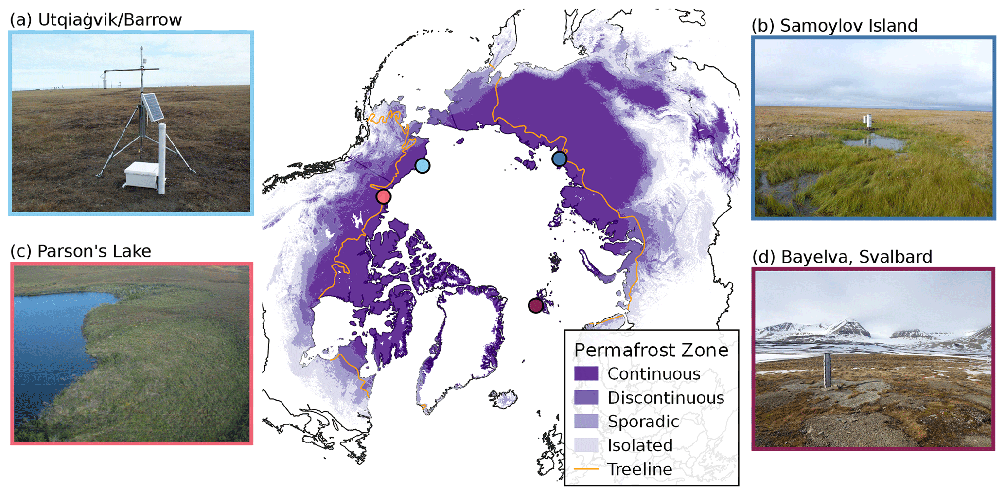
Figure 1 Map of the four study sites overlaid on the permafrost extent from Obu et al. (2019). Orange marks the tree line (Brown et al., 1997). Photos are reprinted/adapted with permission from published documentation for each site: Barrow (Bar, 2021), Samoylov Island (Boike et al., 2019), Bayelva (Boike et al., 2018a), and Parson's Lake (Smith et al., 2018) (permission granted by Open Government License - Canada: https://open.canada.ca/en/open-government-licence-canada, last access: 22 August 2023).

These computational challenges in inverse modeling are naturally also relevant for transient models of permafrost processes which typically require solving one or more partial differential equations governing heat and water flow in the forward evaluation (Westermann et al., 2023; Tubini et al., 2021; Riseborough et al., 2008; Nicolsky et al., 2007). Finding computationally feasible methods for performing simulation-based inference is, therefore, a key methodological challenge in investigating the thermal state of permafrost with numerical models. However, relatively few studies to date have attempted to address this challenge. Romanovsky and Osterkamp (1997) used an analytical equilibrium model to invert air and soil temperatures measured at three sites in northern Alaska; Nicolsky et al. (2009) later used a traditional variational approach to invert measured soil temperatures with a numerical model of 1D heat conduction similar to the one used in our study. Harp et al. (2016) analyzed the effects of soil property uncertainties on permafrost thaw using the null-space Monte Carlo (NSMC) method applied to the Advanced Terrestrial Simulator (ATS) of Coon et al. (2019). More recently, Garnello et al. (2021) used Bayesian methods to calibrate the GIPL permafrost model (Jafarov et al., 2012) and make long-term permafrost thaw projections.

The primary objectives of this study are (i) to analyze the relationship between near-surface air and permafrost temperature trends observed at several research stations in the Arctic continuous permafrost zone and (ii) to relate observed borehole temperature trends to plausible changes in latent heat over the last 2 decades via ensemble inversion of a transient heat conduction model with phase change. In both cases, we focus on the probabilistic quantification of uncertainty using Bayesian inference. To overcome the aforementioned computational challenges in solving the inverse problem for heat conduction, we apply a recently developed particle-based sampling method for approximate posterior inference (Garbuno-Inigo et al., 2020) suitable for complex numerical models. We apply our methods to four different sites (Fig. 1) located in different climate zones in northeastern Siberia, Svalbard, northern Alaska, and northwestern Canada, where long-term borehole temperature records (> 10 years) as well as stratigraphic information are available.

Boike et al. (2019)Boike et al. (2018a)ECCC (2011)Theisen (2022)

Table 1 Summary of climatological conditions for each of the four study sites included in this work. Air temperatures (for January and July) are monthly averages, rainfall refers to total annual unfrozen precipitation, and max snow depth refers to the maximum annual snow depth. Data are averaged over the reference period. All quantities were computed directly from published data for the indicated time period unless otherwise specified. Climatology data for Parson's Lake are taken from the nearest available long-term observation station at Trail Valley Creek, which is about 37 km southeast of the borehole site.

^a  Computed using ECCC data from the later time period of 2015–2021. ^b Estimated visually from Fig. 5 of Burn and Kokelj (2009) for the earlier time period of 2000–2007. ^c Estimated visually from Fig. 6 of Shiklomanov et al. (2010) for the earlier time period of 1994–2010.

2 Study sites

In order to cover a broad range of environmental and climatic conditions, we apply our inverse modeling method to borehole and meteorological data obtained from sites in four different regions within the continuous permafrost zone. Figure 1 shows the geographical locations of each site along with photos of the local landscape. Table 1 provides a summary of available data on the long-term climatology of each site for a given reference period.

2.1 Samoylov

The Samoylov research station (Boike et al., 2019) lies on Samoylov Island (72^∘22^′11.76^′′ N, 126^∘28^′51.0^′′ E) within the Lena River delta at the edge of the Laptev Sea in northeastern Siberia. The region is characterized by ice-wedge polygonal tundra, dense vegetation coverage, large water bodies, and sandy ice-rich sediment. The site lies within the continuous permafrost zone and has permafrost reaching depths of 400 to 600 m below the surface (Grigoriev, 1960) with active layer thickness ranging from 0.3 to 0.7 m. Recent surface temperature reconstructions show that the permafrost has been subjected to substantial warming over the last century (Kneier et al., 2018). The station provides automated monitoring of surface and climate conditions in addition to an instrumented 27 m borehole drilled in 2006 from which hourly ground temperature measurements are available up until September 2021.

2.2 Bayelva

The Bayelva station (Boike et al., 2018a) is located on the Brøgger peninsula of the island of Spitsbergen, Svalbard, approximately 3 km from the small research village of Ny-Ålesund (78^∘55^′14.987^′′ N, 11^∘50^′3.156^′′ E). The West Spitsbergen Current helps to maintain comparatively mild seasonal temperatures in the area around Ny-Ålesund. The unglaciated coastal areas are known to have continuous permafrost extending to depths as deep as 100 m (Humlum, 2005), with active layer depths of 1 to 2 m. The site is situated on top of a hill, and the surrounding landscape is characterized by patterned permafrost ground and sparse (50 %–60 %) vegetation coverage. The soils on the hill range from silty loam to silty clay with some marine deposits, while coarser-grained silty sands can be found in the surrounding area. The site includes an instrumented 9 m deep borehole with hourly measurements of ground temperatures dating back to 2009.

2.3 Parson's Lake

The Parson's Lake, “T5 Upland”, borehole site (Smith et al., 2018; Wolfe et al., 2010) is situated east of the Mackenzie delta, northeast of Inuvik in the Northwest Territories and within the continuous permafrost zone of northern Canada (68^∘57^′29.879^′′ N, 133^∘50^′17.159^′′ W). The region is classified as dwarf birch tundra with dense vegetation coverage and large water bodies (Burn and Kokelj, 2009). Soils in the area are mostly coarse-grained sand in the upper layers, with finer-grained silty-clay soils in the deeper layers (>1 m). Soil cores also show evidence of excess ground ice in moderate amounts (approximately 5 %–25 % volumetric content) 1 to 2 m below the surface. Permafrost extends down to 100 m or more in the outer delta area (Allen et al., 1988), and active layer thickness typically ranges from 0.35 to 0.65 m. The site features a roughly 10 m deep borehole with daily mean ground temperature measurements dating back to 2006.

2.4 Barrow

The Barrow North Meadow Lake 2 (NML2) borehole site (71^∘19^′14.07^′′ N, 156^∘38^′57.587^′′ W) is situated near the village of Utqiaġvik (formerly known as Barrow), which lies at the northernmost point of Alaska along the Arctic coast. The surrounding landscape is characterized by drained thaw lakes and upland tundra consisting of gravel and silty soils with highly variable moisture and organic content in the active layer (Shiklomanov et al., 2010). The region lies within the continuous permafrost zone and is known to have permafrost extending down to 300 m (Brewer, 1958) or more below the surface, with highly variable active layer thickness ranging from 0.1 to 1.0 m. The upper permafrost layer is fairly ice rich, with ground ice content as high as 50 %–75 % by volume in some areas. In this work, we use data from a borehole at the North Meadow Lake 2 (NML2) site, where instrumented daily average soil temperature measurements in the permafrost layer down to 15 m are sparsely available for the time frame 2012–2017, and annual measurements down to 47 m are available from 2009–2021 (Bar, 2021; Nelson et al., 2008; Romanovsky et al., 2002). We were only able to make use of the annual measurements below the assumed depth of zero annual amplitude in this study due to a large number of data gaps in the instrumented measurements.

3 Methods

3.1 Bayesian inference

The Bayesian approach to statistics provides a natural framework for inferring unobserved quantities of interest while simultaneously accounting for their associated uncertainties (Berliner, 2003). This is accomplished via Bayes' rule:

$$\begin{array}{}\text{(2)}& \begin{array}{rl}& p\left(X\right|Y)={\displaystyle \frac{p\left(Y\right|X\left)p\right(X)}{p\left(Y\right)}}\\ & \text{ with }p\left(Y\right)=\underset{x\in X}{\int }p\left(Y\right|X=x\left)p\right(X=x)\mathrm{d}x,\end{array}\end{array}$$

which can be seen as a generic formula for obtaining the so-called posterior distribution of an unobserved quantity X given observations Y. The prior distribution p(X) reflects our uncertainty about X a priori (i.e., before observing Y), while the likelihood p(Y|X) measures how well the model's predictions agree with the observations Y. In this work, Y values are temperature measurements, typically sampled over time and/or space, whereas X values are unknown model parameters or unobserved physical quantities such as soil properties, active layer thickness, or the ratio of sensible to latent heat. The overall objective is then to obtain the posterior distribution p(X|Y) of these unknown parameters given the temperature measurements which quantifies not only the best-fitting parameter settings but also the associated modeling uncertainties.

Difficulties in the practical applications of Bayesian methods have historically arisen from the intractability of the integral in the denominator of Eq. (2), often referred to as the marginal likelihood p(Y). Advances over the last few decades in numerical sampling methods such as Markov Chain Monte Carlo (MCMC) (Hoffman and Gelman, 2014; Bishop, 2006; Duane and Kogut, 1986) which sidestep the need to compute the marginal likelihood, as well as a general increase in available computing power, have made Bayesian methods significantly more accessible. However, computing the likelihood still requires running the forward model given each set of parameters; for many scientific and simulation-based models, this incurs a significant computational burden.

3.2 Trend analysis

As a preliminary step of our study, we analyze trends in mean annual air and permafrost temperatures for each study site. For Samoylov, Bayelva, and Barrow, we use daily averaged in situ air temperature data where available and bias-corrected ERA5-Land (Mu noz-Sabater et al., 2021) 2 m air temperature in all years in the study period (2000–2020) where in situ observations are unavailable. The bias-correction procedure for air temperature closely follows the empirical quantile mapping method of Piani et al. (2010), in which the empirical quantiles of both the model (reanalysis) and observational data are computed over some reference period (in this study, we use the full time period for which observations are available); the model data are then mapped to the corresponding quantiles of the observations. We deviate slightly from this procedure by only applying the correction to values within the observed (in situ) temperature range to avoid artificially clipping extreme temperatures in the reanalysis product. For the Parson's Lake borehole site, we use air temperatures from ERA5-Land without any correction since we were not able to find long-term in situ measurements near the station.

Due to the small sample size of our annual data (fewer than 20 years at all sites), we analyze air and permafrost temperature trends with a Bayesian robust linear trend model. We choose the Student's t distribution as the likelihood due to its longer tails which allow for more tolerance of unusually cold or warm years without severely affecting the overall trend (Lange et al., 1989) . We use standard, weakly informative prior distributions for each parameter, with the exception of the slope μ₁ to which we assign a mildly informative unit Gaussian. This is justified by the fact that annual average change in temperature near and below the surface can be reasonably expected to fall well below 1 K per annum. The specification of the full probability model can be found in Appendix B1.

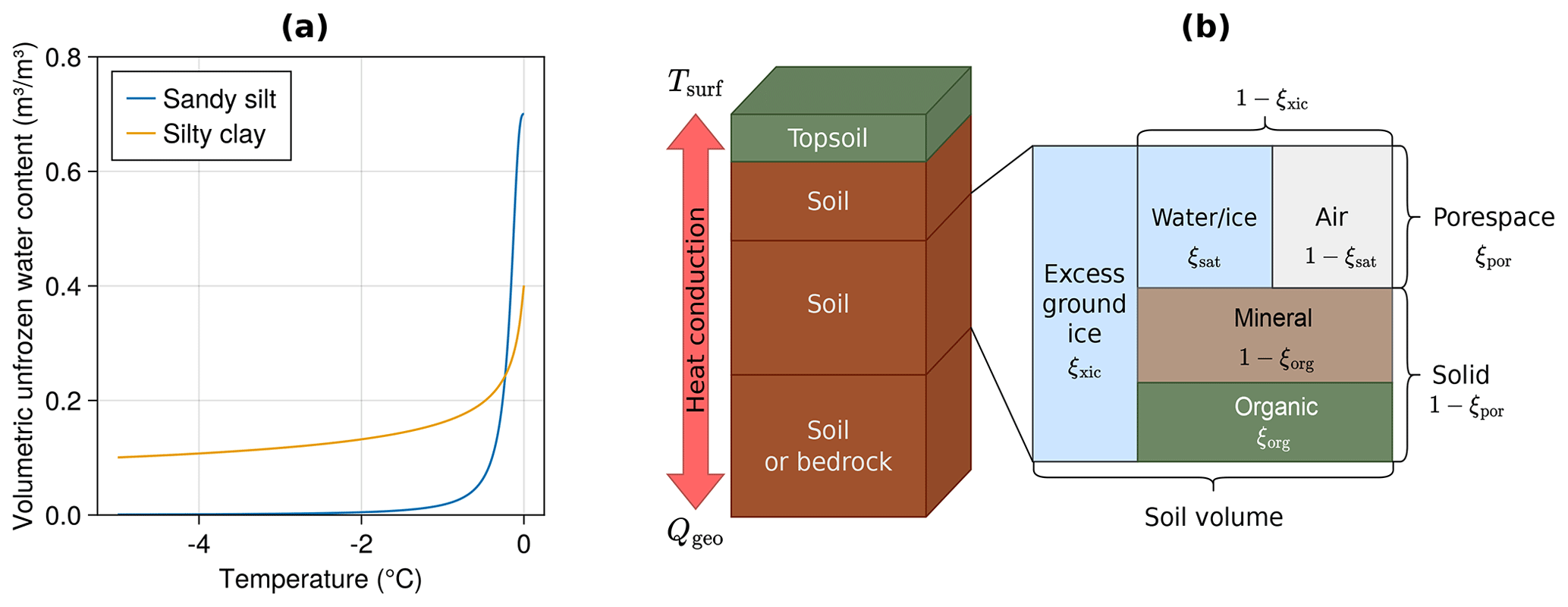
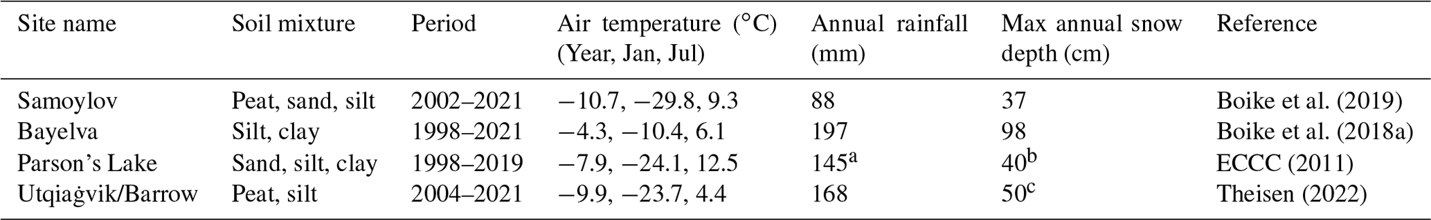
Figure 2 Illustrations of key concepts employed by our heat transfer model: (a) examples of soil freezing characteristic curves used in our model for two different soil textures. The curves shown in here are based on observations from Samoylov Island (sandy silt) and Bayelva (silty clay). (b) Simplified graphical representation of a four-layer stratigraphy configuration of the transient heat conduction model. The model uses stacked, homogeneous soil layers, where each layer is represented as a partitioning of excess ice, pore space, and solid material. The actual number of soil layers in the stratigraphy varies between sites. T_surf and Q_geo represent the surface temperature and geothermal heat flux boundary conditions, respectively. Each ξ represents the characteristic fraction of one soil component.

3.3 Transient heat conduction model

3.3.1 Subsurface heat transfer

In order to simulate the diffusion of heat in permafrost soils, we use a transient heat conduction model based on the same numerical procedures and parameterizations of CryoGrid (Westermann et al., 2023, 2016), which solves the 1-dimensional nonlinear heat equation with phase change:

$$\begin{array}{}\text{(3)}& {\displaystyle \frac{\partial H\left(T\right)}{\partial t}}={\displaystyle \frac{\partial }{\partial z}}\left[k\left(T\right){\displaystyle \frac{\partial T(z,t)}{\partial z}}\right],\end{array}$$

where H(T) [J m⁻³] is the discrete enthalpy function over d finite volumes Δ_i(z), $i=\mathrm{1},\mathrm{\dots },d$ is defined on the depth domain z∈𝒵 with $\mathcal{Z}=[\mathrm{0}\mathrm{m},\mathrm{1000}\mathrm{m}]$, and k(T) [$\mathrm{W}{\mathrm{m}}^{-\mathrm{1}}{\mathrm{K}}^{-\mathrm{1}}$] is the (temperature dependent) thermal conductivity. Note that Eq. (3) is in so-called mixed form, i.e., the conserved quantity (enthalpy) is linked to the diffused quantity (temperature) by a nonlinear constitutive relationship. We can recover temperature from enthalpy via the following nonlinear system:

$$\begin{array}{}\text{(4)}& T={\displaystyle \frac{H-L\mathit{\theta }\left(T\right)}{C\left(\mathit{\theta }\right(T\left)\right)}},\end{array}$$

which can be solved using standard numerical methods, such as Newton iteration, or approximated using a pre-calculated interpolant. Here, θ(T) represents the SFCC for a given soil type. In this work, we use the SFCC specified by Eqs. (21)–(23) in Dall'Amico et al. (2011) (see Fig. 2a and Appendix B2.1 for details), which is derived from the widely used van Genuchten (1980) soil-water retention equations.

Since no general solution exists for Eq. (3) with arbitrary boundary conditions, numerical approximation is necessary in order to find a solution for T(z,t). We discretize the spatial domain according to a fixed, non-uniform grid with the smallest grid cell spacing of 0.05 m from the surface down to a depth of approximately 4 m and a pseudo-exponentially increasing grid spacing thereafter.

We specify the soil stratigraphy for each site as stacked homogeneous layers, where the soil in each layer is parameterized according to the four characteristic fractions: excess ground ice (ξ_xic), natural porosity (ξ_por), saturation (ξ_sat), and organic content (ξ_org). From these independent fractions, the volumetric soil constituent fractions for excess ground ice (θ_x), pore water and ice (θ_wi), air (θ_a), and mineral and organic soil fraction (θ_m,θ_o) can be computed via recursive partitioning of the volume, as shown in Fig. 2 and described in Appendix B2.1. Note that, while excess ground ice is represented through super-saturation of the soil volume (effectively just increasing the porosity), soil and water displacement from ground ice melt and hydraulic processes are neglected, and the total water and ice content θ_wi+θ_x is assumed to remain constant throughout the simulation.

3.3.2 Initial and boundary conditions

Accurate simulation of the surface energy balance, snow dynamics, and surface hydrology is notoriously difficult and comes with many sources of uncertainty in landscapes with very heterogeneous surface characteristics (Langer et al., 2011a, b). An empirical alternative to approximate the bulk thermal effect of these complex surface processes is to use n factors (Riseborough et al., 2008; Lunardini, 1978), which attempt to approximate the long-term deviation of surface temperature from air temperature via lumped scaling factors:

$$\begin{array}{}\text{(5)}& \begin{array}{rl}& n_{\mathrm{F}}={\displaystyle \frac{{\text{FDD}}_{\text{soil}}}{{\text{FDD}}_{\text{air}}}},n_{\mathrm{T}}={\displaystyle \frac{{\text{TDD}}_{\text{soil}}}{{\text{TDD}}_{\text{air}}}},\\ & \text{FDD}=\underset{t_{\mathrm{1}}}{\overset{t_{\mathrm{2}}}{\int }}{T}^{-}\left(t\right)\mathrm{d}t,\text{TDD}=\underset{t_{\mathrm{1}}}{\overset{t_{\mathrm{2}}}{\int }}{T}^{+}\left(t\right)\mathrm{d}t,\end{array}\end{array}$$

where $T^{+}\left(t\right)=\text{max}\left(T\right(t),\mathrm{0}{}^{\circ }\mathrm{C})$, and $T^{-}\left(t\right)=\text{min}\left(T\right(t),\mathrm{0}{}^{\circ }\mathrm{C})$. Note that FDD and TDD represent the commonly known freezing and thawing degree days. The resulting dimensionless factors $n_{\mathrm{F}},n_{\mathrm{T}}\in [\mathrm{0},\mathrm{1}]$ can be used to approximate insulated surface temperatures by scaling the instantaneous air temperature:

$$\begin{array}{}\text{(6)}& T_{\text{surf}}\left(t\right)=\left\{\begin{array}{ll}{n}_{\mathrm{F}}\left(t\right)T_{\text{air}}\left(t\right)& T_{\text{air}}\left(t\right)\le \mathrm{0}\\ n_{\mathrm{T}}\left(t\right)T_{\text{air}}\left(t\right)& T_{\text{air}}\left(t\right)>\mathrm{0}.\end{array}\right.\end{array}$$

We use T_surf, with T_air derived from the same, bias-corrected ERA5-Land air temperature record described in Sect. 3.2, as the Dirichlet upper boundary condition for temperature in the transient heat conduction model. In order to account for possible decadal scale changes in surface conditions, the seasonal n factors n_F and n_T are reparameterized as time-dependent, piecewise linear functions with knots at five pre-defined time points: 2000, 2005, 2010, 2015, and 2020. The values at each knot, e.g., $n_{\mathrm{F}}^{\left(\mathrm{0}\right)}$, $n_{\mathrm{F}}^{\left(\mathrm{1}\right)}$, $n_{\mathrm{F}}^{\left(\mathrm{2}\right)}$, $n_{\mathrm{F}}^{\left(\mathrm{3}\right)}$, and $n_{\mathrm{F}}^{\left(\mathrm{4}\right)}$ (same for n_T), are varied as unknown parameters, thereby allowing T_surf, which is not generally known or measured reliably, to be adapted according to the observed borehole temperatures. The geothermal heat flux at the lower boundary (1 km below the surface) is set to 0.053 W m⁻² and can generally be assumed to have a negligible effect on the decadal timescales considered in this work (Hermoso de Mendoza et al., 2020).

The initial temperature profile at each site is parameterized similarly to the n factors as a piecewise linear function between five knots: $\mathrm{0}\mathrm{m},{\widehat{T}}_{\text{air}}\left(t_{\mathrm{0}}\right))$, (z_ALT,T₁), (z_ZAA,T₂), $(z_{\text{base}},\mathrm{0}{}^{\circ }\mathrm{C})$, and (1000 m,T₃), where ${\widehat{T}}_{\text{air}}\left(t_{\mathrm{0}}\right)$ is the average annual air temperature for the first simulation year, and T₁, T₂, T₃, and z_base (i.e., depth of the permafrost base) are varied as unknown parameters. z_ALT and z_ZAA nominally refer to the initial active layer thickness and depth of zero annual amplitude, respectively; these values are set based on rough estimates from the relevant literature for each site. Each simulation additionally includes a 20 year “spin-up” period (1979–1999) which is excluded from the analysis. The spin-up period allows the thermal state of the upper subsurface layers to reach dynamic equilibrium with the forcing, thereby minimizing the impact of the initial condition on the upper 10 m of the soil profile. Conversely, the parametric initial state prior to the spin-up period broadly accounts for first-order uncertainty in the initial temperature profile of the deeper layers which would otherwise require much longer spin-up periods (centuries or millennia) to equilibrate.

Figure 3 ISO standard flowchart showing a simplified overview of the inversion workflow using ensemble Kalman sampling (EKS).

3.4 Inverse modeling

3.4.1 Theoretical framework

The inverse problem of recovering some unobserved sequence of states x_1:τ from observations y_1:τ over τ temporal samples can be expressed via Bayes' rule (Evensen et al., 2022):

$$\begin{array}{}\text{(7)}& \begin{array}{rl}p({\mathit{x}}_{\mathrm{1}:\mathit{\tau }},\mathit{\varphi }|{\mathit{y}}_{\mathrm{1}:\mathit{\tau }},{\mathit{s}}_{\mathrm{1}:\mathit{\tau }})\propto & p\left({\mathit{y}}_{\mathrm{1}:\mathit{\tau }}\right|{\mathit{x}}_{\mathrm{1}:\mathit{\tau }},\mathit{\varphi },{\mathit{s}}_{\mathrm{1}:\mathit{\tau }})\\ & \times p\left({\mathit{x}}_{\mathrm{1}:\mathit{\tau }}\right|\mathit{\varphi },{\mathit{s}}_{\mathrm{1}:\mathit{\tau }}\left)p\right(\mathit{\varphi }),\end{array}\end{array}$$

where ϕ∈Φ represents the parameters characterizing the underlying hydrothermal processes in a dynamical model of the state variables x, and s_1:τ represents any set of relevant exogenous variables (e.g., meteorological forcings, energy sources or sinks), which define the boundary conditions of the system. The objective of the inverse problem is then to obtain samples from the posterior distribution $p({\mathit{x}}_{\mathrm{1}:\mathit{\tau }},\mathit{\varphi }|{\mathit{y}}_{\mathrm{1}:\mathit{\tau }},{\mathit{s}}_{\mathrm{1}:\mathit{\tau }})$ over model states x_1:τ and parameters ϕ. We assume that the parameters ϕ are independent of the exogenous inputs s_1:τ, and we neglect possible uncertainty arising from s_1:τ, thereby allowing us to ignore the corresponding density p(s_1:τ) in Eq. (7). The likelihood $p\left({\mathit{y}}_{\mathrm{1}:\mathit{\tau }}\right|{\mathit{x}}_{\mathrm{1}:\mathit{\tau }},\mathit{\varphi },{\mathit{s}}_{\mathrm{1}:\mathit{\tau }})$ determines how likely the observational data are, given a sequence of states produced by the forward model, while the distribution $p\left({\mathit{x}}_{\mathrm{1}:\mathit{\tau }}\right|\mathit{\varphi },{\mathit{s}}_{\mathrm{1}:\mathit{\tau }})$, sometimes referred to as the “process model”, relates a particular set of parameters ϕ to a sequence of states x_1:τ. In our approach, we focus on probabilistically modeling parametric uncertainty induced by the prior $p\left(\mathit{\varphi }\right)={\prod }_{i=\mathrm{1}}^m{p}_i\left({\mathit{\varphi }}_i\right)$ over m model parameters which encode a priori site-specific knowledge (e.g., soil characteristics and surface conditions) where available. We neglect uncertainty in the process model, thereby assuming the model states to be a deterministic function of the parameters. Additional theoretical discussion of the inverse modeling method can be found in Appendix B3.1.

3.4.2 Approximate inference via ensemble Kalman sampling

Evaluation of the likelihood $p\left({\mathit{y}}_{\mathrm{1}:\mathit{\tau }}\right|{\mathit{x}}_{\mathrm{1}:\mathit{\tau }},\mathit{\varphi },{\mathit{s}}_{\mathrm{1}:\mathit{\tau }})$ requires a forward simulation of the heat transfer model described in Sect. 3.3 given the parameters ϕ which incur a substantial computational cost. To mitigate this issue, we employ a recently developed, probabilistic variant of the widely used ensemble Kalman inversion (EKI) (Iglesias et al., 2013) algorithm called ensemble Kalman sampling (EKS) (Garbuno-Inigo et al., 2020) to efficiently produce approximate samples from the posterior over model parameters, $p\left(\mathit{\varphi }\right|{\mathit{y}}_{\mathrm{1}:\mathit{\tau }},{\mathit{s}}_{\mathrm{1}:\mathit{\tau }})$. EKS assumes that the observed borehole temperatures can be represented as

$$\begin{array}{}\text{(8)}& T_{\text{obs}}=\left(g_{\mathrm{T}}{}^{\circ }f\right)\left(\mathit{\varphi }\right)+\mathit{\eta },\end{array}$$

where g_T is the forward map from the model states produced by f to comparable temperature observations, and $\mathit{\eta }\sim \mathcal{N}(\mathrm{0},{\mathrm{\Sigma }}_{\mathrm{T}})$ is observation noise with zero mean and assumed covariance Σ_T. Additional inputs to f, such as forcing data, are assumed to be independent of ϕ and are here suppressed for brevity. EKS requires the prior distribution over parameters to be a multivariate Gaussian, so we must first construct a bijective function $\mathit{\gamma }:\mathrm{\Phi }\to \mathrm{\Psi }$ that maps the m-dimensional parameters ϕ∈Φ to values ψ∈Ψ with unbounded support on the real line. The approximate prior for EKS is then specified as $\mathit{\psi }\sim p\left(\mathit{\psi }\right)=\mathcal{N}({\mathit{\mu }}_{\mathit{\psi }},{\mathrm{\Sigma }}_{\mathit{\psi }})$. The key insight behind the EKS algorithm is that an ensemble of parameter values {ψ⁽ⁱ⁾} sampled from an initial density (i.e., the prior) can be transformed into samples from the (approximate) posterior distribution by treating them as a stochastic system of interacting particles. Their dynamics are then governed by the overdamped Langevin equation:

$$\begin{array}{}\text{(9)}& {\displaystyle \frac{\partial {\mathit{\psi }}^{\left(i\right)}}{\partial t}}=-\mathrm{\nabla }\mathcal{L}\left({\mathit{\psi }}^{\left(i\right)}\right)+\sqrt{\mathrm{2}}R\left(t\right),\end{array}$$

where ℒ(ψ) is the log-likelihood of the unconstrained parameters ψ with respect to the observations and R(t) is an m-dimensional Brownian motion. It can be shown that this interacting particle system then converges to the posterior density over an infinite time horizon, where “time” here refers to that of the particle diffusion rather than physical time in the forward model. We refer the reader to Garbuno-Inigo et al. (2020) for further details about the EKS algorithm and iteration procedure.

The main advantage of EKS over other commonly used numerical sampling methods, such as Markov Chain Monte Carlo (MCMC), is that it is a parallelizable “ensemble” or particle-based method which requires a relatively small number of iterations to converge (typically fewer than 30). In contrast, most MCMC methods require thousands of sequential (and therefore non-parallelizable) iterations. This makes EKS more attractive for use cases such as the inverse modeling problem considered in this work where the computational cost of likelihood is relatively high. EKS also avoids the need to design complex, multi-stage model reduction and/or emulation procedures such as those used for Bayesian evidential learning (Hermans et al., 2018). This comes at the cost, however, of finding only a Gaussian approximation to the “true” posterior.

We apply the implementation of EKS published by the authors (Constantinou et al., 2022) to our heat conduction model using borehole data obtained from each of the four sites described in Sect. 2. We use an ensemble of size N=512, and we initialize the ensemble by sampling N parameter vectors ϕ from the prior p(ϕ). We iterate EKS for at most 30 iterations or until two units of particle diffusion “time” are reached. Further details on the problem setup for EKS are given in Appendix B3.2.

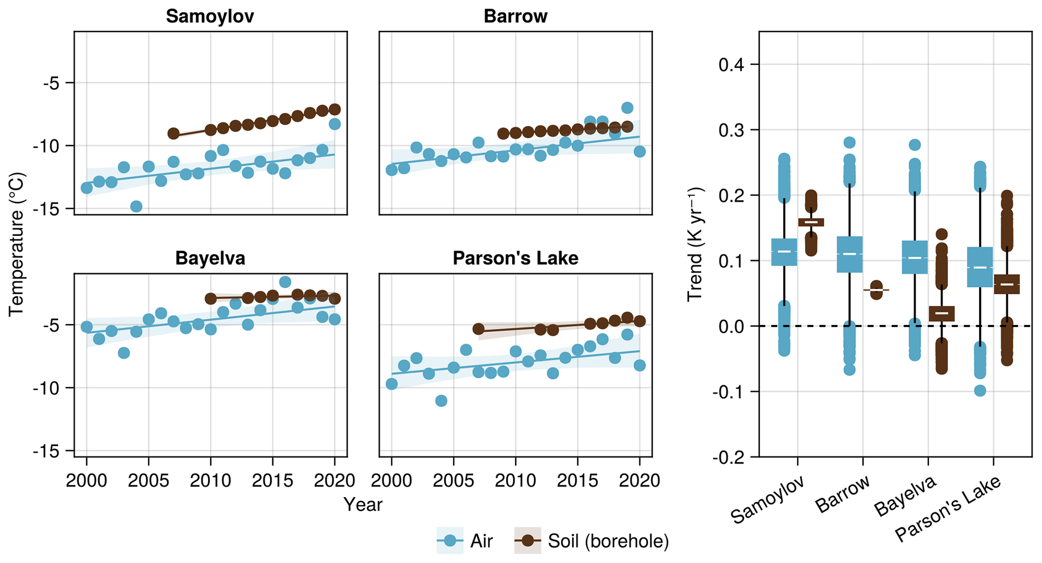
Figure 4 Trend analysis of observed mean annual temperature trends in air vs. soil at all sites. Permafrost temperatures are from borehole measurements as close as possible to the depths of zero annual amplitude: 20.75 m (Samoylov), 20.0 m (Barrow), 9.0 m (Bayelva), and 9.82 m (Parson's Lake). The dots represent observed mean annual temperatures at each location. For air temperature, the adjusted ERA5-Land temperature reanalysis record is used where observations are not available. Trend lines and their corresponding 95 % central credible intervals are obtained via numerical sampling from a robust trend model.

4 Results

4.1 Observed permafrost and air temperature trends

The results of the trend analysis over the 20 year time period (2000–2020) described in Sect. 3.2 are shown in Fig. 4. The left panel shows the observed air and permafrost temperatures over time alongside the trend lines sampled from the posterior. The solid line represents the posterior mean, while the shaded region shows the 95 % central credible interval (CCI), which represents the interval between the 2.5 % and 97.5 % percentiles of the posterior samples. The boxplots in the right panel show summaries of the posterior distribution over slopes of the trend line, which can be more naturally interpreted as the average annual change in temperature over the observed time period. The whiskers of the boxplot span the range $[q_{\mathrm{1}}-\mathrm{1.5}R,q_{\mathrm{3}}+\mathrm{1.5}R]$, where q₁ and q₃ are the first and third quartiles, respectively, and R is the interquartile range. All probabilities given in this section refer to posterior probabilities calculated from MCMC samples, with Monte Carlo adjusted standard error (MCSE) strictly less than $\mathrm{2}\times {\mathrm{10}}^{-\mathrm{3}}$ in all cases.

Our analysis shows very strong evidence of increasing air temperatures (i.e., $\mathrm{Pr}({\mathit{\mu }}_{\mathrm{1}}>\mathrm{0})>\mathrm{0.99}$ for all sites), with the slope of the trend line μ₁ ranging from 0.09 K yr⁻¹ (95 % CCI 0.00 to 0.18 K yr⁻¹) at Parson's Lake to 0.11 K yr⁻¹ (0.04 to 0.18 K yr⁻¹) at Samoylov Island. In comparison, mean annual permafrost temperatures near the depth of zero annual amplitude show similarly strong evidence of warming at three of the four sites: temperatures rose by approximately 0.16 K yr⁻¹ (0.14 to 0.18 K yr⁻¹) on Samoylov Island, 0.06 K yr⁻¹ (0.05 to 0.06 K yr⁻¹) at Barrow, and 0.06 K yr⁻¹ at Parson's Lake (0.02 to 0.11 K yr⁻¹). For Bayelva, the observed deep permafrost temperatures show a far milder warming trend of approximately 0.02 K yr⁻¹ (−0.02 to 0.05 K yr⁻¹) and are considerably less conclusive ($\mathrm{Pr}({\mathit{\mu }}_{\mathrm{1}}>\mathrm{0})\approx \mathrm{0.85}$).

Next, we investigate the observed difference between soil and air temperature trends across sites. We find that soil temperature trends are generally lower than air temperature trends at both Barrow ($\mathrm{Pr}({\mathit{\mu }}_{\mathrm{1}}^{\text{(soil)}}<{\mathit{\mu }}_{\mathrm{1}}^{\text{(air)}})\approx \mathrm{0.90}$) and Bayelva ($\mathrm{Pr}({\mathit{\mu }}_{\mathrm{1}}^{\text{(soil)}}<{\mathit{\mu }}_{\mathrm{1}}^{\text{(air)}})\approx \mathrm{0.98}$). This relationship is less evident at the Parson's Lake borehole site ($\mathrm{Pr}({\mathit{\mu }}_{\mathrm{1}}^{\text{(soil)}}<{\mathit{\mu }}_{\mathrm{1}}^{\text{(air)}})\approx \mathrm{0.68}$), with ground temperatures warming at a comparable rate to air temperatures. In stark contrast to the other sites, borehole measurements at Samoylov show deep soil temperatures warming on average 0.05 K yr⁻¹ (35 %) faster than air temperatures with fairly high confidence ($\mathrm{Pr}({\mathit{\mu }}_{\mathrm{1}}^{\text{(soil)}}>{\mathit{\mu }}_{\mathrm{1}}^{\text{(air)}})\approx \mathrm{0.92}$).

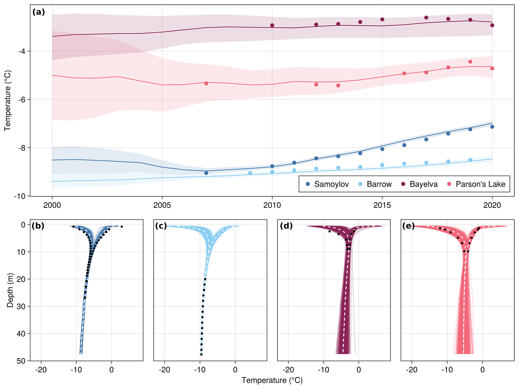
Figure 5 (a) Modeled vs. observed mean annual ground temperatures at sensors which are as close as possible to the depth of zero annual amplitude: 20.75 m (Samoylov), 20.0 m (Barrow), 9.0 m (Bayelva), and 9.82 m (Parson's Lake). The dots indicate observed annual borehole temperatures, and the lines represent the mean of the ensemble predictions. The shaded regions cover 95 % of the ensemble predictions. (b–e) Minimum and maximum annual temperature profiles at 2 m and below for the years 2020 (Samoylov, Bayelva, Parson's Lake) and 2019 (Barrow), observed (dots) vs. model ensemble predictions, with the white dotted line indicating the median over the ensemble.

4.2 Ensemble inversion

Modeled vs. observed annual ground temperatures over the 20 year simulation period are shown in Fig. 5. The predicted temperatures from each ensemble member represent an approximate sample from the posterior predictive distribution. The solid line in Fig. 5a is the ensemble mean temperature prediction, while the shaded regions show the 95 % CCI over all ensemble members, i.e., the interval into which 95 % of the predicted values for each ensemble member fall. Figure 5b–e show the observed vs. ensemble minimum and maximum annual temperatures for the last year in the simulation period where observations are available. We can see in Fig. 5 that, for both Samoylov and Parson's Lake, the ensemble predicted temperatures fit the observed borehole temperatures relatively well, although the 2020 annual min–max ground temperature curve for Samoylov (Fig. 5b) indicates a slight bias in the min–max temperature range for the upper part of the profile affected by seasonal variation. The ensemble temperatures for Bayelva also appear reasonable, though there is a clear warm bias in the winter apparent in the temperature profile. The corresponding min–max temperature curves (Fig. 5d) reveal a substantial amount of ensemble variation in the annual minimum and maximum temperature despite fairly modest variation in the ensemble mean at 9 m. This is also apparent in the 2020 ensemble temperature profile for Parson's Lake (Fig. 5e). There is much more variation in the deeper part of the soil profile (i.e., below 10 m) for both of these sites in comparison to Samoylov and Barrow (Fig. 5b–e), likely due to the lack of deeper borehole measurements available to constrain the initial temperature profile.

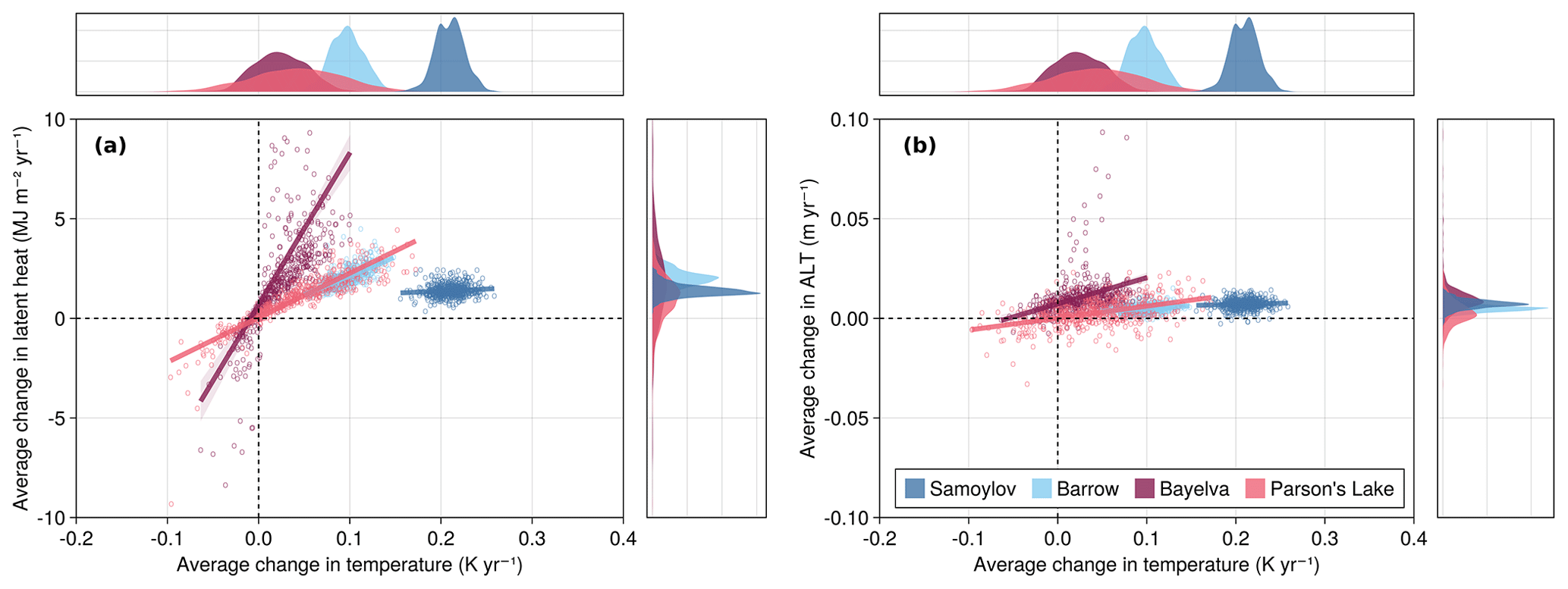
Figure 6 Joint densities of modeled mean annual change in latent heat (a) and active layer thickness (b) vs. mean annual change in ground temperature for all sites. Each point represents a single member of the fitted ensemble. Energy content and temperature are integrated over all grid cells in the upper 10 m of the soil profile. The density plots on the top and right panels of each plot show the marginal densities. In both plots, a small number of points from Bayelva exceed the upper y-axis limit and thus are not shown.

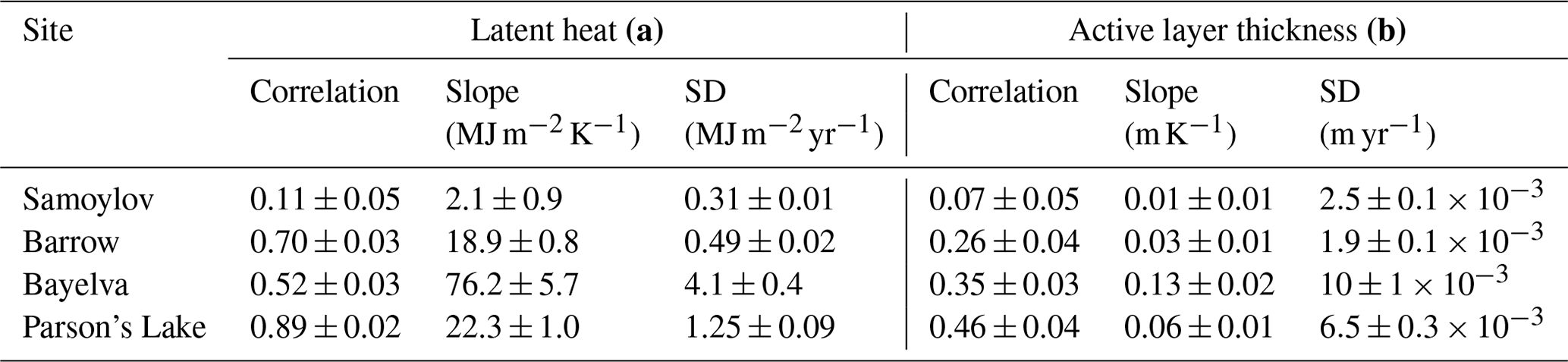
Figure 6 shows the joint and marginal distributions of average annual change in modeled latent heat (Fig. 6a) and ALT (Fig. 6b) with average integrated ground temperature, i.e, the weighted average of grid cell temperatures, for each of the four sites. Here, average annual change is defined as the slope of the least squares trend line fitted over the entire simulation period (2000–2020) for each ensemble member. We integrate the predicted temperatures and energy contents over the upper 10 m of the soil profile. The choice of 10 m is arbitrary but is motivated by the availability of measurements from Bayelva and Parson's Lake. Note that, since the model assumes constant hydrological conditions, changes in latent heat can be directly attributed to phase change. The density plots on the top and right panels of Fig. 6 show the ensemble marginal densities of temperature and latent heat change, respectively. Each point in the plot represents the slope of the least squares trend line for one ensemble member after fitting with EKS. The lines in the plot show the linear relationship between changes in temperature and latent heat across all ensemble members. Table 2 shows the correlation and regression coefficients associated with each linear fit. Stronger positive correlations between temperature and latent heat trends imply higher sensitivity of permafrost thaw to changes in sensible heat uptake.

Table 2 Summary statistics (Pearson correlation, slope of the least squares line, and standard deviations) for the linear relationships shown in Fig. 6 with respect to both latent heat vs. temperature (a) and ALT vs. temperature (b). Means and standard errors are bootstrap estimates using 10 000 resamples from the ensemble outputs.

We can see in Fig. 6a that all three sites with silty or clay-like soils (i.e., Barrow, Bayelva, and Parson's Lake) exhibit a much stronger positive correlation between change in latent heat and temperature. Samoylov, in contrast, shows little to no correlation despite the comparatively rapid increase in ground temperature. Figure 6b shows a clear difference in how changes in ALT correlate with changes in temperature between the two warmer sites, Parson's Lake and Bayelva, versus the two colder sites, Samoylov and Barrow. The simulations for both Parson's Lake and Bayelva show a stronger positive correlation between increasing ALT and increasing temperature, whereas for the colder sites this correlation is weaker (Barrow) or virtually non-existent (Samoylov). Both warmer sites also show more overall variability across the ensemble in both latent heat and ALT trends, with standard deviations of the trend slopes more than double those of the cold sites.

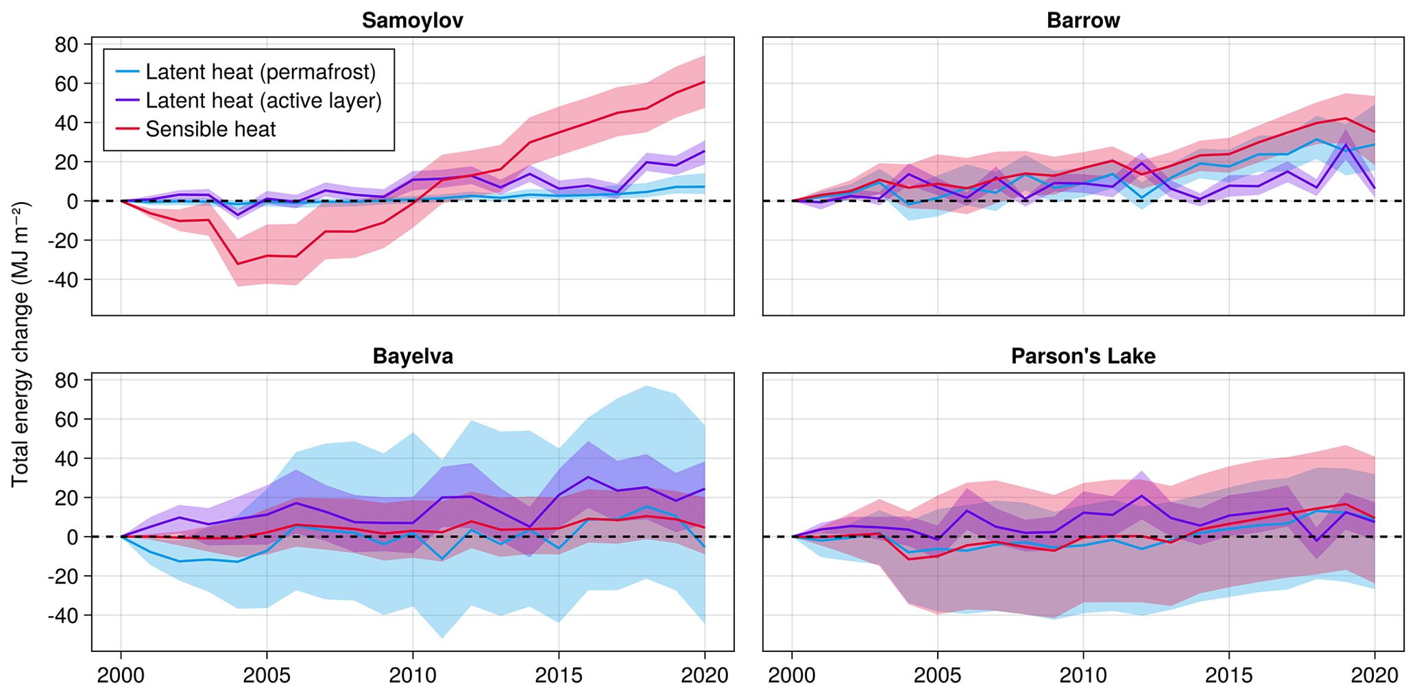
Figure 7 Total change in energy partitions (upper 10 m of soil profile) since the beginning of the simulation period. Energy is partitioned into three categories: latent heat in frozen grid cells (i.e., cells with maximum annual temperature T_max < 0 ^∘C), latent heat in the active layer (T_max ≥ 0 ^∘C), and sensible heat. Solid lines show the median energy change, while the shaded regions show the 95 % CCI over the ensemble. Changes in heat capacity due to phase transitions in pore water and ice are excluded here from the sensible heat component in order to better isolate the relative contributions of temperature change vs. phase change.

Lastly, Fig. 7 shows the long-term change in the mean annual energy contents of the upper 10 m of the soil profile over the full simulation period (2000–2020) for each site. The energy storage is partitioned into three parts: latent heat stored in permafrost, i.e., grid cells that have a maximum annual temperature below 0 ^∘C; latent heat stored in the active layer; and sensible heat due to temperature change. The solid lines show the median energy change over all fitted ensemble members, and the shaded regions indicate the corresponding 95 % CCI. The categorization of a grid cell as being in the permafrost or active layer for the latent heat partitions is not constant; i.e., as the active layer grows or shrinks over time, the categorization of each grid cell based on maximum annual temperature changes as well. This means that the change in latent heat for each partition is attributable not only to the thawing and freezing of water but also to the migration of grid cells between the two partitions.

Note that the sensible heat as defined in Eq. (1) depends on the liquid water content via the heat capacity (see Eq. B6 in the Appendix). For the purpose of more clearly visualizing the relative contributions of temperature (sensible) vs. latent heat change in Fig. 7, we employ a non-conservative formulation of the sensible heat: $H_{\mathrm{s}}\left(T\right)=T\times c_{\mathrm{i}}$, where c_i is the volumetric heat capacity of ice, thereby effectively removing the dependence of sensible heat on the unfrozen water content. This alternative formulation allows us to more clearly see the relative contributions of temperature change and latent heat to the long-term evolution of the thermal state.

5 Discussion

5.1 Estimating trends in observed permafrost and air temperatures

Numerous recent studies have highlighted warming trends observed in borehole sites all across the Arctic (Smith et al., 2022; Chen et al., 2021; Biskaborn et al., 2019; Romanovsky et al., 2007). The results of our trend analysis are broadly consistent with Biskaborn et al. (2019), who reported average decadal changes in permafrost temperatures of 0.39 ± 0.15 K dec⁻¹ for 53 GTN-P boreholes across the continuous permafrost zone between 2007 and 2016, which translates into an average annual change of roughly 0.02 to 0.05 K yr⁻¹. Observed warming trends at the Samoylov Island borehole site in the Lena River delta (Siberia) over the longer period of 2007–2020 are unusually extreme (also noted by Biskaborn et al. (2019) for the same borehole), with a mean annual change of 0.16 K yr⁻¹, while observed changes at the Bayelva site near Ny-Ålesund (Svalbard) fall towards the lower end of the expected range with a mean annual change of 0.02 K yr⁻¹. For air temperature, Biskaborn et al. (2019) report average changes of 0.86 ± 0.84 K dec⁻¹ (0.02 to 0.17 K yr⁻¹) across the continuous permafrost zone from 2007–2016 using spatially interpolated 2 m air temperatures from reanalysis products. This is consistent with the results of our analysis which show mean air temperature trends ranging from 0.09 K yr⁻¹ at Parson's Lake to 0.11 K yr⁻¹ on Samoylov Island. This discrepancy in observed permafrost temperature trends between these two sites, despite similar changes in air temperature, indicates considerable uncertainty in how permafrost is responding to the changing climate that is likely attributable to other factors. For example, thicker and/or less dense snow cover can accelerate permafrost warming by insulating the ground against rapid drops in air temperature characteristic to autumn and early winter, thereby delaying the refreezing of the active layer (Park et al., 2015). Additionally, soil thermal properties such as the bulk conductivity and freezing characteristics due to soil texture can also play a significant role in modulating the effects of surface temperature changes (Nicolsky and Romanovsky, 2018; Romanovsky and Osterkamp, 2000; Riseborough, 1990). Both of these factors, among others, can significantly affect energy uptake in the subsurface and, ultimately, the current and future thermal state of permafrost in Arctic regions (Smith et al., 2022; Langer et al., 2022).

The results of this trend analysis motivate our inverse modeling study by demonstrating clear, localized differences and substantial uncertainty in how the permafrost thermal regime at these four sites is responding to long-term changes in air temperature. We argue that this can be at least partially attributed to factors affecting the uptake of latent heat in the subsurface such as soil freezing characteristics as well as historical climatology. We discuss in the following sections how our inverse modeling results suggest that both of these factors are major sources of uncertainty in making inferences about the changing thermal state of permafrost.

5.2 Variability and biases in modeled permafrost temperatures

There is substantial variability in modeled temperatures over the simulation period (2000–2020) even after using EKS to calibrate the model ensemble to borehole measurements (Fig. 5). We see, for example, significant differences in the overall range of predicted temperatures between sites. This can be partially explained by both differences in air temperature variability (Fig. 4) as well as in the depths at which temperature observations are available; e.g., the deepest sensors at the Bayelva and Parson's Lake sites are at 9 m and 9.82 m, respectively, whereas both Barrow and Samoylov have much deeper measurements available near the depth of zero annual amplitude where there is little to no impact from seasonal variation. We present additional experiments exploring the sensitivity of our inversion method to available sensor depths in the Supplement (Sect. S1 in the Supplement). We find that the inclusion or exclusion of measurements at various depths has a fairly predictable effect on the results of the analysis; i.e., the inclusion of data at additional sensor depths generally improves the fidelity of the predicted temperatures at these depths and reduces the associated uncertainty. However, the results suggest that constraining the model using only deep measurements, as we do for the Barrow site, may lead to overestimation of warming at depths closer to the surface.

The general agreement between the modeled and observed mean annual temperatures in Fig. 5 suggests that the fitted model ensemble can nonetheless provide a plausible estimate of the permafrost's thermal state at all four sites, subject to some uncertainties. There are, however, some clear discrepancies between modeled and observed permafrost temperatures which should be considered, particularly in the final year temperature profiles for Samoylov and Bayelva. For Samoylov, the ensemble annual temperature range of the permafrost in the upper 10 m of the ground is slightly too narrow, showing a warm bias in the winter (0.6 ± 0.3 K averaged over the profile) and a cold bias ($-\mathrm{0.7}\pm \mathrm{0.2}$ K) in the summer for the last simulation year of 2020 (Fig. 5b). This may be due to the thermal conductivities of the upper layers being too low, thereby over-insulating the lower layers. Furthermore, while many of the soil properties are varied in the ensemble, the stratigraphy itself (i.e., the number and thickness of layers) is not, which could also be responsible for such biases. The wintertime warm bias for Bayelva (1.5 ± 0.5 K) may also be due to our assumption of static hydrology, which fails to capture the effects of seasonal changes in soil moisture on the subsurface thermal regime. The release of latent heat during freezing slows the propagation of cold surface temperatures, thereby delaying the refreezing of the active layer in early winter (Romanovsky and Osterkamp, 2000). When unfrozen water is removed from the active layer due to drainage or evapotranspiration, the latent heat stored in this water is removed as well. The result is that cold temperatures can propagate faster in the wintertime since a higher fraction of this energy is diffused as sensible heat. This would therefore serve as a possible explanation for the warm bias in the model at this site. We can see quite clearly from the volumetric water content measurements shown in Fig. 3 of Boike et al. (2018a) that soil saturation levels in the active layer vary substantially (10 % to 20 %) both within and between years. It has also been well established by previous studies that hydrological conditions have a substantial effect on the subsurface thermal regime on Svalbard (Westermann et al., 2011; Roth and Boike, 2001). Accounting for water fluxes may therefore be necessary to more accurately reproduce thermal conditions at Bayelva and other sites with similar characteristics. Nevertheless, we believe the results of our inversion procedure agree well enough with temperature observations to provide insight into how the thermal state of permafrost at each site may have evolved over the last 2 decades.

5.3 Linking temperature trends to changes in permafrost thaw

The clear differences between the joint distributions for each site in Fig. 6 have substantial implications for the interpretation of permafrost temperature trends. Firstly, it is evident that the freezing characteristics of the soil, represented in our inversion method through variation of the soil freezing characteristic curve parameters, have a substantial impact on the relationship between trends in temperature and latent heat. This is made most apparent in Fig. 6a by the presence of a strong linear relationship between latent heat change and temperature change at Barrow (18.9 ± 0.8 MJ K⁻¹, Table 2) but not at Samoylov (2.1 ± 0.9 MJ K⁻¹). Both sites are in many ways similar; they both have historically very cold permafrost (below −8 ^∘C near the depth of annual amplitude), an insulating organic layer at the surface, and similar amounts of annual snow cover (Table 1). One of their key differences, however, is that the soils in the Barrow region tend to have higher silt content (Romanovsky and Osterkamp, 2000) which exhibits freezing characteristics that lead to larger amounts of unfrozen water at subzero temperatures. The result is that, as permafrost close to the active layer warms, a larger amount of energy is consumed as latent heat, thereby slowing the rate of temperature change near the freezing front and effectively insulating the colder permafrost below (Nicolsky and Romanovsky, 2018). This is also seen clearly in Fig. 7, where the estimated change in latent heat storage of permafrost for the Barrow simulations clearly dwarf that of Samoylov by up to a factor of 10.

The joint density of active layer thickness trends with temperature trends in Fig. 6b tells a similar story. As with latent heat, simulations for the three sites with silty or clay-like soils in the permafrost layers show the strongest positive correlation with ALT, while those for Samoylov show little to none. However, the correlation and effect size for the Barrow simulations (0.26 ± 0.04 m K⁻¹ and 0.03 ± 0.01 m K⁻¹, respectively, Table 2) are notably lower than those for the two warmer sites, Bayelva (0.35 ± 0.03 m K⁻¹ and 0.13 ± 0.02 m K⁻¹) and Parson's Lake (0.46 ± 0.06 m K⁻¹ and 0.06 ± 0.01 m K⁻¹). This is likely due to the colder, deep permafrost at Barrow acting as a heat sink and thereby offsetting the effects of warming closer to the surface.

The vast majority of ensemble members for both Samoylov and Barrow show clear warming trends, whereas the marginal distributions of temperature change for Bayelva and Parson's Lake are more diffuse and tend to be closer to zero. This is broadly consistent with the hypothesis of Riseborough (1990) as well as the more recent findings of Nitzbon et al. (2023), i.e., that regions with warmer permafrost may show less detectable subsurface warming while actually being at higher risk for degradation. The two warmer sites (particularly Bayelva) also tend to show similar or larger changes in latent heat content and ALT even with relatively little change in temperature; this is likely due to a larger portion of energy being consumed as latent instead of sensible heat. This hypothesis is further supported by Fig. 7, which shows sensible heat as the clear dominant component of long-term energy change at Samoylov and, to a lesser extent, also at Barrow. We discuss this further in Sect. 5.4.

The wider range of modeled ALT and latent heat change at both Bayelva and Parson's Lake (Figs. 6 and 7) indicates higher uncertainty in modeling the thermal dynamics of warmer permafrost. This can be attributed to higher sensitivity to soil properties, initial conditions, and changes in surface conditions and soil water content. This sensitivity is in large part due to the nonlinear effects of the freeze curve on the thermal dynamics, especially in deep permafrost (i.e., near the depth of zero annual amplitude) where thermal gradients are smaller and heat diffuses more slowly.

A small number of ensemble members for both of these warmer sites lie in the upper left quadrants of Fig. 6a and b, i.e., where there is a positive trend in latent heat or ALT despite average ground temperatures actually declining over the simulated time period. Similarly, some ensemble members for these two sites fall into the lower two quadrants, indicating a decrease in latent heat or ALT with some parameter settings. This is in contrast to the two colder sites, Samoylov and Barrow, where nearly all ensemble members show positive trends in temperature, latent heat, and ALT. This underscores two features of warmer permafrost: (i) that observed temperature trends (or lack thereof) should be interpreted with caution, as there is substantial uncertainty inherent in associated changes in latent heat, and (ii) that the sensitivity of warmer permafrost to climatic change is highly dependent on soil thermal properties, most notably the soil freezing characteristics. Soils which retain more unfrozen water at temperatures below 0 ^∘C may delay thawing and refreezing due to the nonlinear effects of latent heat (Nicolsky and Romanovsky, 2018).

5.4 Latent heat as a subsurface energy sink

While it is clear that Arctic permafrost is warming (Smith et al., 2022; Chen et al., 2021; Biskaborn et al., 2019; Smith et al., 2010), the latent heat effect acts on a larger scale as both an energy source and sink (Nitzbon et al., 2023; Cuesta-Valero et al., 2023), which can have the effect of masking long-term temperature changes in the climate signal (Nicolsky and Romanovsky, 2018; Riseborough, 1990), thereby introducing considerable uncertainty into the long-term implications of warming across the Arctic. Figure 7 visualizes this uncertainty by comparing long-term changes in the partitioned subsurface energy budget across sites. There is a clear contrast between the two colder sites, Samoylov and Barrow, in the upper panels versus the two warmer sites, Bayelva and Parson's Lake, in the lower panels. For the colder sites, sensible heat change plays a more dominant role with both the median and full 95 % CCI of the ensemble showing a positive trend for most of the simulation period. The decrease in sensible heat at Barrow in the last simulation year, 2020, is likely due to the unusually large drop in air temperature which can be seen in Fig. 4. In contrast, both warmer sites show latent heat change playing a larger role.

Long-term change in latent heat uptake also differs between the colder and warmer sites. For both Samoylov and Barrow, a vast majority of ensemble members show an increase in latent heat both in the permafrost partition (i.e., grid cells where maximum annual temperatures are below zero) as well as in the active layer. This points to both a deepening active layer (consistent with Fig. 6) as well as to warming permafrost. For sites like Barrow with silty soil, the notably larger increase in permafrost latent heat storage also implies a transition of the permafrost into a kind of “mushy” (partially frozen) state as temperatures increase into the critical region of the soil freezing characteristic curve, where liquid water is present at temperatures below the nominal melting point.

Both Bayelva and Parson's Lake show a much larger range of possible trajectories for latent heat storage over the ensemble. Notably, however, the 95 % credible range for both sites (especially Bayelva) spans a wide range of possible trajectories for latent heat storage in the permafrost. Latent heat in the active layer, however, appears to be likely increasing at both sites. This may be attributable to expansion of the active layer in combination with delayed sensible warming of permafrost due to the latent heat effect. Crucially, both warmer sites also consist of a mixture of more silty and clay-like soils which are characterized by larger amounts of unfrozen water content at temperatures well below the melting point (Fig. 2a). One interesting difference even between the two warmer sites is the relative contribution of latent heat change in the permafrost layer (light blue in Fig. 7) versus sensible heat (light red). The larger variation in this latent heat component at Bayelva appears to be due to two factors: (i) warmer permafrost temperatures in the upper 10 m (Fig. 5) and (ii) differences in the soil stratigraphies; e.g., our model configuration for Parson's Lake has on average 10 % lower porosity from 1.75 to 10 m depth which translates into less overall latent heat by volume. Furthermore, the more heterogeneous mixture of soil textures (and therefore freezing characteristics) in the Parson's Lake stratigraphy, as well as the higher variability in air temperature (Fig. 4), results in a higher overall contribution of sensible heat to the subsurface energy balance. Our analysis here highlights how the nonlinear effect of the soil freezing characteristics on permafrost thermal dynamics limits the reliability of temperature measurements in understanding the impact of climate warming on the thermal state of permafrost.

5.5 Limitations

While we are confident that the ensemble inversion method and results presented in this study provide valuable insight into the relationship between air temperature trends, subsurface temperature trends, and permafrost thaw, there are several limitations of our methodology which are important to address.

1. Neglected subsurface processes. The transient heat conduction model described in Sect. 3.3 is capable of accurately simulating heat conduction with phase change at a relatively high spatial resolution. However, it neglects several processes such as water infiltration and percolation, excess ice melt and subsidence, and lateral exchange of heat and water in the subsurface. In particular, the assumption that soil water content remains constant over the simulation period precludes factoring in the effects of long-term wetting or drying on the thermal properties (and therefore the thermal regime) of the ground closer to the surface. This could potentially alter the thermal dynamics of the ground in two ways: firstly, unfrozen water which is transported out of the pore space and not replaced can be seen as effectively removing energy from the system, thereby altering the energy balance of the ground. Secondly, drier soils with higher air content will necessarily be less conductive, thereby becoming an insulator for deeper layers against further warming and cooling. However, the assumption of static hydrological conditions allows us to more easily compare changes in the partitioning of latent vs. sensible heat between sites (Fig. 7). We further note that for Samoylov, which is typically waterlogged, no substantial wetting or drying has been reported during the simulation period (Boike et al., 2019).

2. Simplified parameterization of surface processes. Our model does not explicitly represent surface processes such as radiative and turbulent heat fluxes, water bodies, vegetation, and snow dynamics but represents them in bulk via n factors (see Sect. 3.3.2). Thus, inter-annual variability in surface conditions is not effectively represented, and meteorological forcings other than air temperature are not taken into account, thereby neglecting potentially valuable sources of information that could serve as additional constraints on the inverse problem. We might expect, for example, some of the inter-annual fluctuations to be explained by changes in snow or cloud cover. The inclusion of additional surface processes, however, also brings with it a whole range of additional uncertainties from both the forcing data as well as from the additional parameterizations.

3. Selection and calibration of prior distributions. The model parameter priors employed in this work are loosely derived from both auxiliary data sources as well as field work and published values in the literature (see Appendix B3.3 for further discussion). However, the general lack of precise error and uncertainty estimates for some model parameters (e.g., soil properties) makes the construction of prior distributions difficult. It is evident from the marginal posterior plots (Figs. A2–A5) that many parameters show minimal change from their priors. This may be the result of overly narrow prior densities or may simply indicate that annual temperature measurements do not provide sufficient information to update them. Furthermore, it is very likely that many parameters are, in reality, highly correlated in the joint distribution, which we are currently unable to account for in the prior. Prior distributions which are more informative or more realistic will help the inversion method converge faster and improve the reliability of the resulting posterior samples in making inferences about the system under study. We nevertheless emphasize that even imperfect (but plausible) prior distributions still do a better job of accounting for uncertainty than the point estimates of parameter values typically provided by non-probabilistic calibration methods.

4. Statistical limitations. While EKS provides a computationally efficient alternative to MCMC for drawing samples from the posterior, it is nevertheless an approximation which provides a theoretical guarantee of convergence to the posterior measure only over an infinite “time” horizon (i.e., iterations of the algorithm) (Garbuno-Inigo et al., 2020). Furthermore, the empirical results presented by the authors of EKS indicate that the method underestimates posterior variance (and thus uncertainty) on a finite time horizon unless the ensemble is very large. More recent work by Cleary et al. (2021) has attempted to circumvent this problem by performing exact posterior inference on emulated predictions produced by a surrogate model. Additionally, EKS requires a priori specification of the sampling distribution covariance Σ_T, which is not, in general, known. A fully Bayesian treatment of the inversion problem would include these Σ_T (or equivalent) parameters in the posterior distribution. This would have the benefit of producing posterior samples where the predictive distribution is well calibrated; i.e., the 95 % prediction interval should actually cover approximately 95 % of the observations in the calibration period, therefore providing a built-in measure of the degree to which the model is capable of explaining the observations.

These limitations provide a wide range of directions for future work; e.g., points 1 and 2 could be addressed simply by incorporating additional physical processes into the model, such as those described in Westermann et al. (2023). However, this typically comes at a heavy computational cost, limiting the feasibility of running large ensembles over longer time periods spanning multiple decades, centuries, or millennia. We are optimistic that recent advancements in simulation-based inference (Cranmer et al., 2020) and/or machine-learning-based approximations of the likelihood (Thibaut et al., 2022; Hermans et al., 2018) may be able to address this challenge, as well as those described by issues 4 and 5. We also see potential in applying an inversion method similar to the one outlined in this work at a larger, circum-Arctic scale, perhaps by leveraging more efficient formulations of the heat conduction model such as those proposed by Tubini et al. (2021) or Langer et al. (2022). The greatest challenge here is the limited availability of high quality borehole data at a global scale, despite the ongoing efforts of collaborative data collection and publication projects such as GTN-P (Biskaborn et al., 2015).

6 Conclusions

In this work, we analyzed trends in annual air and permafrost temperatures at four different sites in the Arctic continuous permafrost zone. We found that long-term trends in permafrost temperatures over the study period (2000–2020) varied between the four sites (0.02 to 0.16 K yr⁻¹) more than trends in air temperatures (0.09 to 0.11 K yr⁻¹). In order to investigate what permafrost temperatures can tell us about the thermal state of permafrost, we then applied a recently developed method for ensemble inverse modeling, ensemble Kalman sampling (Garbuno-Inigo et al., 2020), to constrain a transient heat conduction model using long-term borehole temperature measurements from each site. We demonstrated that the response of the subsurface thermal regime to warming at the surface varies substantially between sites based on their historical climatology (i.e., colder versus warmer conditions) as well as the thermal properties of the soil. We found that the degree to which trends in permafrost temperatures correlate with changes in latent heat or active layer thickness depends heavily on both historical climatology and the soil freezing characteristics. In particular, the sensitivity of modeled active layer thickness to changes in temperature were higher for the two sites with warmer permafrost, 6 ± 1 cm K⁻¹ at Parson's Lake in northwestern Canada and 13 ± 2 cm K⁻¹ at Bayelva, Svalbard, versus 3 ± 1 cm K⁻¹ at Utqiaġvik (Barrow) in northern Alaska and a negligible 1 ± 1 cm K⁻¹ at Samoylov Island in northeastern Siberia. Furthermore, we showed that there is substantial uncertainty inherent in relating ground temperature trends to permafrost thaw in areas with warmer permafrost or silty or clay-like soils where the nonlinear effects of latent heat play a much larger role. Our results suggest that currently observed permafrost temperature trends at these sites can be plausibly mapped to a wide range of different thermal states. This is largely due to the lack of information in the temperature signal of permafrost within the critical temperature range where phase change of water occurs. Our findings demonstrate the importance of considering regional differences in soil characteristics and climatology when comparing permafrost temperature trends across sites. Our study also highlights the importance of deep borehole measurements (i.e., deeper than 10 m) in constraining hydrothermal models of permafrost and providing insights into the past and present thermal state of permafrost in the Arctic. Future work will focus on the broader application of probabilistic inversion methods, like the one used in this work, both to more sophisticated permafrost models and at larger spatiotemporal scales.

Appendix A: Additional results

A1 Posterior distributions of wintertime n factors indicate changes in snow cover

The posterior distributions of the wintertime n factors are shown in Fig. A1. Each group of boxplots represents the fitted value of the n factor knot at that year. As described in Sect. 3.3.2, the actual n factor values are interpolated linearly between knots, forming a piecewise linear function over the simulation period. Values for the year 2000 are also applied for all years in the spin-up period (1979–1999). The inter-annual differences between the knots indicate that, in addition to the long-term trend in air temperature, changes in surface conditions are necessary in order to accurately reproduce temperature trends in the borehole data.

Decreasing wintertime n factors for Samoylov between 2005–2020 can be physically interpreted as an increase in surface insulation, typically explained by an increase in snowfall or changes in the timing of the snow covered season. The extent to which long-term snow depth measurements published in Boike et al. (2019) support this hypothesis is unclear, and further validating it will likely require further investigation with models that take into account snow dynamics over shorter timescales. We note, however, that the long-term pattern produced by the n factors serves as a possible explanation for the rapid rate at which deep ground temperatures appear to be warming at the Samoylov Island site (Fig. 4). As discussed in Boike et al. (2019), a new research station was constructed within the immediate vicinity of the borehole site in 2013. The station includes a water delivery system which may act as a wind shield, thereby affecting seasonal snow cover patterns of the area around the borehole. Visual inspection in April of 2016 indicated that snow cover did indeed appear higher since construction of the water supply system (Boike et al., 2019). Thus, there is reason to believe that snow cover has increased at this site, though the cause of this increase remains unclear.

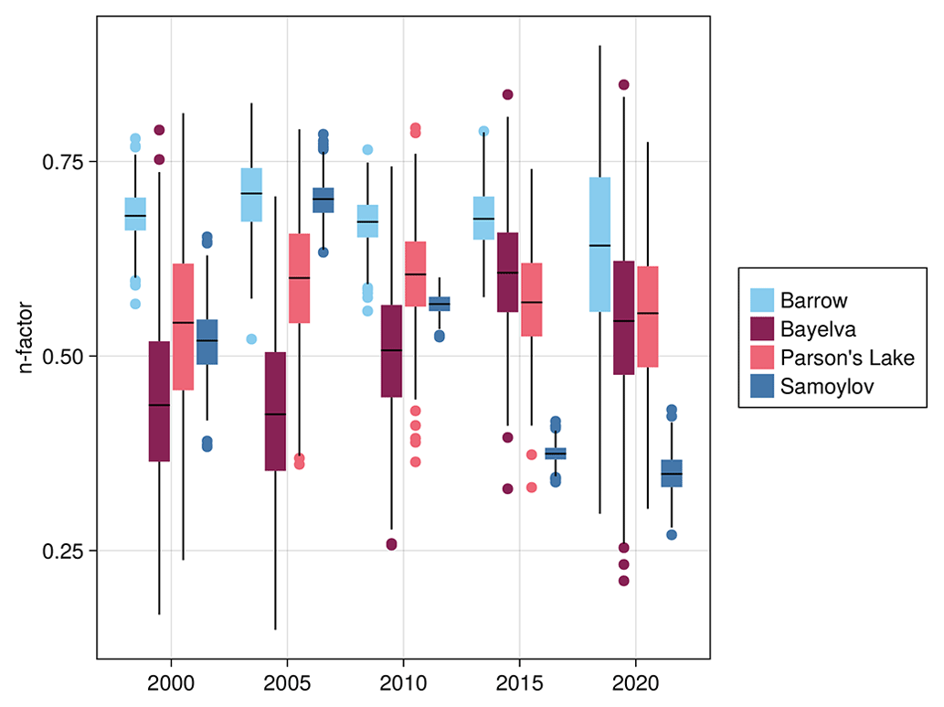
Figure A1 Boxplots showing posterior distributions of wintertime n factors (i.e., applied when T_air(t)≤0) after fitting with EKS.

For the site at Bayelva, Svalbard, the fitted wintertime n factors show the opposite effect, i.e., increasing from roughly 0.4 in 2000 to roughly 0.6 in 2015. This can be interpreted as a reduction in surface insulation, suggesting decreasing snow cover or possibly a longer snow-free season. Long-term snow observations presented by Boike et al. (2018a) verify this hypothesis. The fact that fitted n factor distributions recover this pattern suggests that changes in snow cover are necessary in order to reconcile observed borehole temperatures with warming air temperatures. The higher posterior variance of the Bayelva n factors vs. Samoylov also indicates more uncertainty in the strength of the effect likely due to larger relative contribution of latent heat limiting the information gain from temperature measurements. It is also worth noting that the n factor distributions for Barrow and Parson's Lake show less of a clear temporal pattern, indicating that the observed borehole temperatures can plausibly be explained by air temperature warming alone.

Table A1 Names and descriptions of parameters considered in the ensemble inversion procedure. Some parameters appear multiple times across years or layers as indicated.

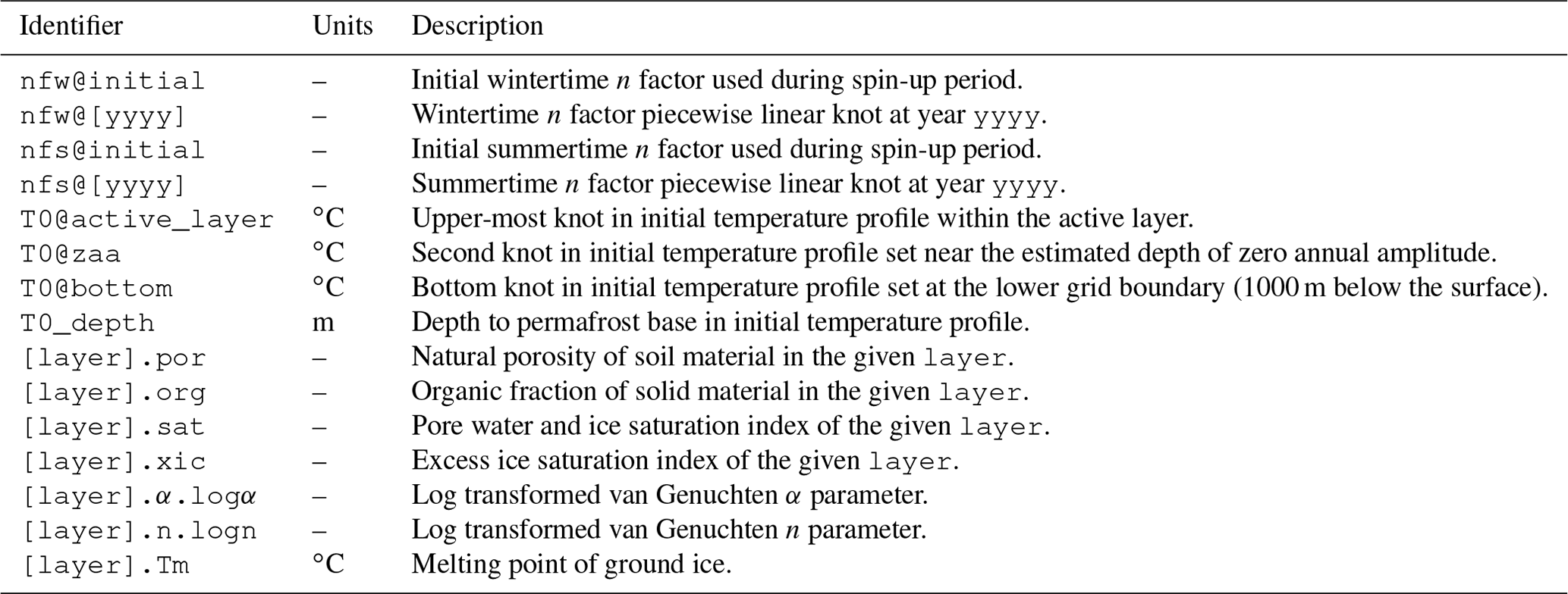
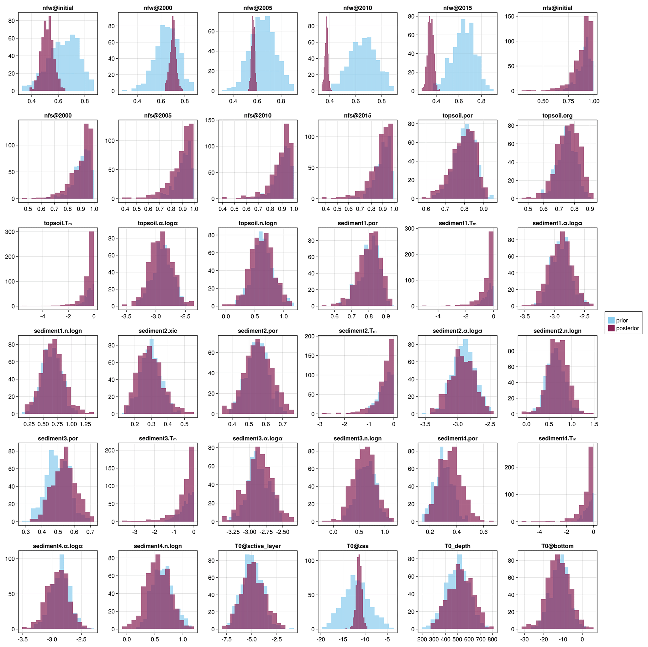
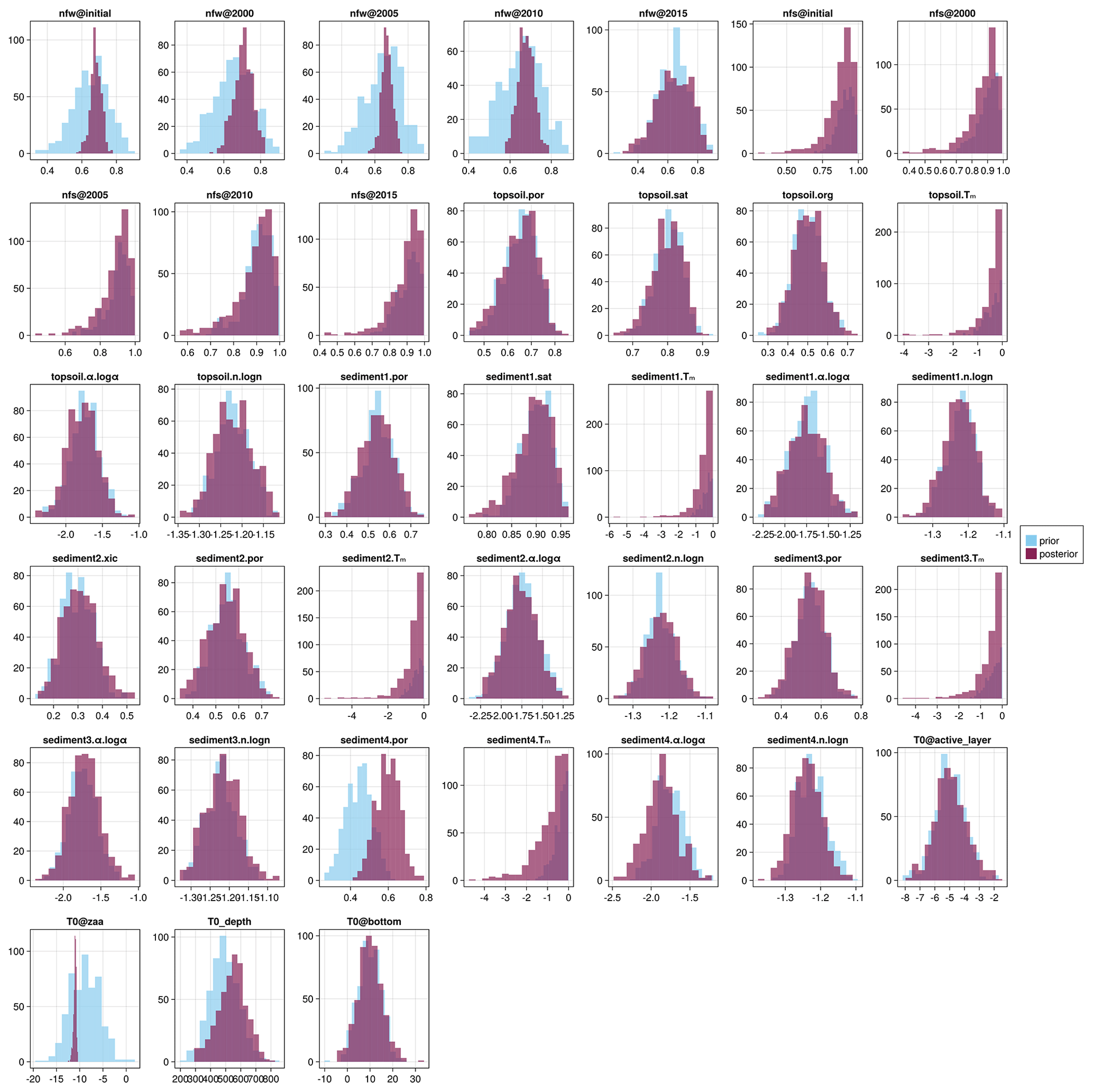
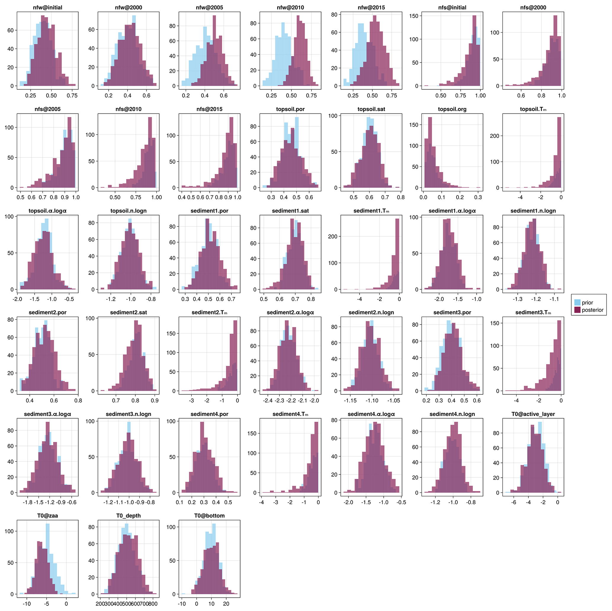
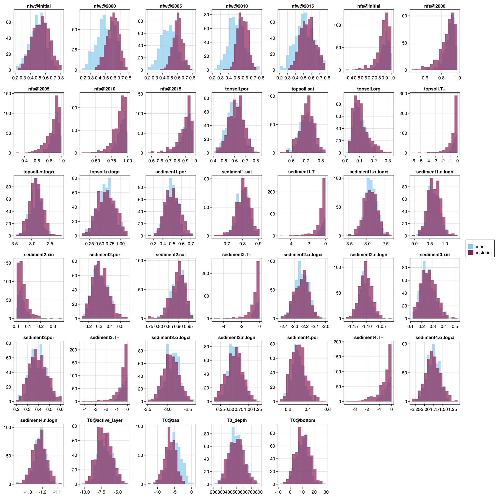
A2 Parameter prior vs. posterior distributions

Histograms of posterior samples (i.e., ensemble members) for all parameters and for each site are presented in Figs. A2 to A5. Parameter names are summarized in Table A1 and generally follow the pattern layer.name[.sub], where name refers to the model parameter being determined and sub refers to the transformed “sub-parameter” where applicable. We use a different naming convention for the forcing and initial condition parameters in order to clearly distinguish them. Note that the set of varied parameters differs slightly between sites due to differences in the stratigraphies; e.g., the excess ground ice parameter is not considered in sites which are assumed (correctly or not) to have no excess ice within the soil column. We can see that, in most cases, the prior and the posterior generally agree, with the only exception being the 2010 and 2015 wintertime n factors for Samoylov. There is clearly a larger reduction in uncertainty of the n factor parameters for both Samoylov and Barrow which is consistent with our findings that sensible heat change dominates at both sites and thus provides a clear signal for changes in the air temperature forcing. Both Parson's Lake and Bayelva generally show minimal change to the prior distribution, likely due to the dominant contribution of latent heat which limits the information gain from temperature measurements.

Figure A2 Fitted ensemble posterior parameter distributions – Samoylov Island.

Figure A3 Fitted ensemble posterior parameter distributions – Barrow.

Figure A4 Fitted ensemble posterior parameter distributions – Bayelva.

Figure A5 Fitted ensemble posterior parameter distributions – Parson's Lake.

Appendix B: Method details

B1 Trend analysis

The annual temperature trend model is specified as

$$\begin{array}{ll}{\displaystyle }{T}_{\mathrm{t}}& {\displaystyle }\sim \mathcal{T}({\mathit{\mu }}_{\mathrm{1}}t+{\mathit{\mu }}_{\mathrm{0}},\mathit{\sigma },\mathit{\nu }),\\ {\displaystyle }{\mathit{\mu }}_{\mathrm{1}}& {\displaystyle }\sim \mathcal{N}(\mathrm{0},\mathrm{1}),\\ {\displaystyle }{\mathit{\mu }}_{\mathrm{0}}& {\displaystyle }\sim \mathcal{N}(\mathrm{0},\mathrm{10}),\\ {\displaystyle }\mathit{\sigma }& {\displaystyle }\sim \text{HalfCauchy}(\mathrm{0},\mathrm{1}),\\ {\displaystyle }\mathit{\nu }& {\displaystyle }\sim \text{Exponential}\left(\mathrm{10}\right),\end{array}$$

where $\mathcal{T}(\mathit{\mu },\mathit{\sigma },\mathit{\nu })$ is the scaled and shifted Student's t distribution with ν degrees of freedom, and t is the zero-centered year. Samples from the posterior distribution $p({\mathit{\mu }}_{\mathrm{1}},{\mathit{\mu }}_{\mathrm{0}},\mathit{\sigma },\mathit{\nu }|T_{\text{obs}},t)$ are obtained via the widely used “No-U-Turn” numerical sampler (NUTS) (Hoffman and Gelman, 2014). We combine 500 independent samples from eight different chains with 2500 discarded adaptation samples to get a total of n=4000 samples for each trend model.

B2 Transient heat conduction model

B2.1 Soil parameterization

The soil constituent fractions by volume are parameterized using the four characteristic fractions: excess ice (ξ_xic), natural porosity (ξ_por), saturation (ξ_sat), and organic solid fraction (ξ_org). The volumetric soil constituent fractions for excess ice (θ_x), pore water and ice (${\mathit{\theta }}_{wi}={\mathit{\theta }}_{\mathrm{w}}+{\mathit{\theta }}_i$), air (θ_a), and mineral and organic content θ_m,θ_o can be computed according to the following linear system:

$$\begin{array}{ll}{\displaystyle }& {\displaystyle }{\mathit{\theta }}_{\mathrm{x}}={\mathit{\xi }}_{\text{xic}},\\ {\displaystyle }& {\displaystyle }{\mathit{\theta }}_{wi}=(\mathrm{1}-{\mathit{\xi }}_{\text{xic}}){\mathit{\xi }}_{\text{por}}{\mathit{\xi }}_{\text{sat}},\\ {\displaystyle }& {\displaystyle }{\mathit{\theta }}_{\mathrm{a}}=(\mathrm{1}-{\mathit{\xi }}_{\text{xic}}){\mathit{\xi }}_{\text{por}}(\mathrm{1}-{\mathit{\xi }}_{\text{sat}}),\\ {\displaystyle }& {\displaystyle }{\mathit{\theta }}_{\mathrm{o}}=(\mathrm{1}-{\mathit{\xi }}_{\text{xic}})(\mathrm{1}-{\mathit{\xi }}_{\text{por}}){\mathit{\xi }}_{\text{org}},\\ {\displaystyle }& {\displaystyle }{\mathit{\theta }}_{\mathrm{m}}=(\mathrm{1}-{\mathit{\xi }}_{\text{xic}})(\mathrm{1}-{\mathit{\xi }}_{\text{por}})(\mathrm{1}-{\mathit{\xi }}_{\text{org}}),\end{array}$$

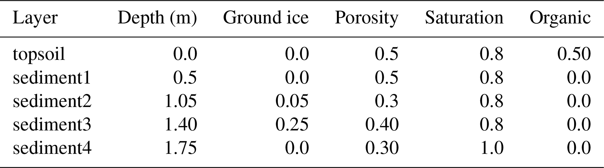
where ${\mathit{\theta }}_{\mathrm{x}}+{\mathit{\theta }}_{wi}+{\mathit{\theta }}_{\mathrm{a}}+{\mathit{\theta }}_{\mathrm{o}}+{\mathit{\theta }}_{\mathrm{m}}=\mathrm{1}$. Mean stratigraphy configurations (i.e., expected value of the prior) used for each site are given in Tables B1 to B4. Note that, in some cases, adjacent layers have identical mean values but are varied independently in the ensemble. Both Bayelva and Parson's Lake also have different freeze curve priors for some layers based on differences in observed soil texture; this is discussed further in Appendix B3.3.

Table B1 Stratigraphy configuration for Samoylov Island borehole simulations.

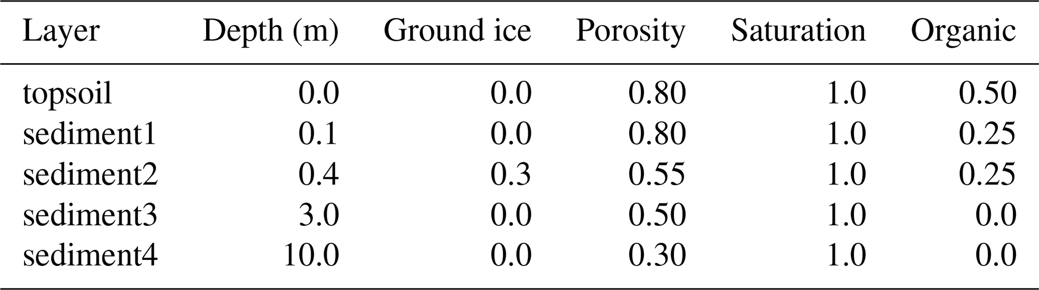
Table B2 Stratigraphy configuration for Bayelva borehole simulations.

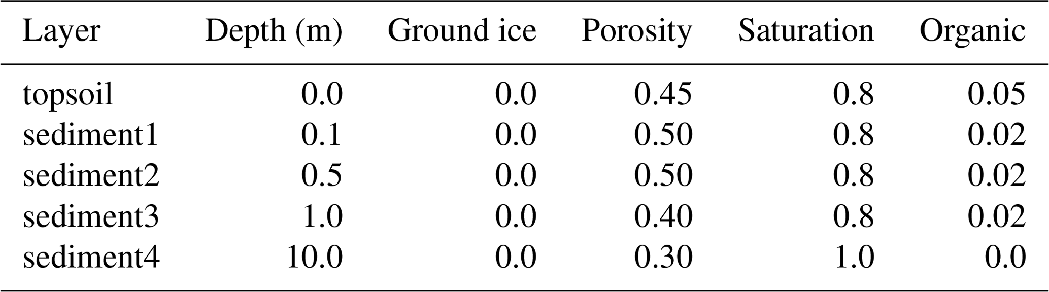
Table B3 Stratigraphy configuration for Barrow borehole simulations.

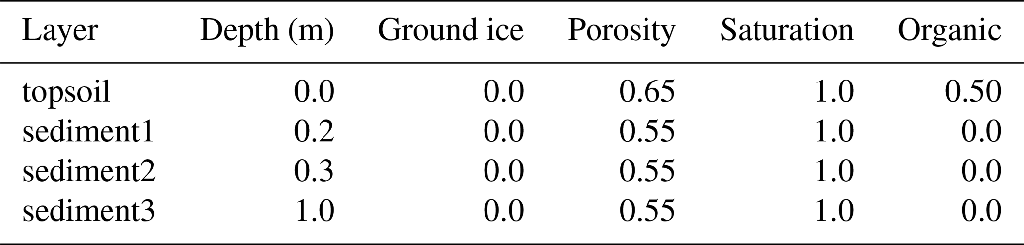
Table B4 Stratigraphy configuration for Parson's Lake borehole simulations.

We use the soil freezing characteristic of Dall'Amico et al. (2011), which is based on the soil water retention equation of van Genuchten (1980). The temperature dependent liquid water matric potential is expressed as

$$\begin{array}{}\text{(B1)}& \mathit{\psi }\left(T\right)=\left\{\begin{array}{ll}{\mathit{\psi }}_{\mathrm{0}}+\frac{L_{\mathrm{f}}}{g{T}^{\ast }}(T-T^{\ast })& T<T^{\ast }\\ {\mathit{\psi }}_{\mathrm{0}}& T\ge T^{\ast },\end{array}\right.\end{array}$$

where ψ₀ is the matric potential due to saturation, L_f = 3.4 × 10⁵ J kg⁻¹ is the specific latent heat of fusion of water, and g = 9.80665 m s⁻² is downward acceleration due to gravity. The critical temperature T^∗ is expressed as a function of the melting temperature T_m and the matric potential:

$$\begin{array}{}\text{(B2)}& T^{\ast }=T_{\mathrm{m}}+{\displaystyle \frac{g{T}_{\mathrm{m}}}{L_{\mathrm{f}}}}{\mathit{\psi }}_{\mathrm{0}}.\end{array}$$

The volumetric liquid water content then follows from the well-known van Genuchten equation (van Genuchten, 1980):

$$\begin{array}{}\text{(B3)}& {\mathit{\theta }}_{\mathrm{w}}={\mathit{\theta }}_{\mathrm{r}}+({\mathit{\theta }}_{\mathrm{s}}-{\mathit{\theta }}_{\mathrm{r}})(\mathrm{1}+(-\mathit{\alpha }\mathit{\psi }\left(T\right){)}^n{)}^{-m},\end{array}$$

where $\mathit{\alpha }\in (\mathrm{0},\mathrm{\infty })$ [m⁻¹], $n\in [\mathrm{1},\mathrm{\infty })$, and $m=\mathrm{1}-\frac{\mathrm{1}}{n}$ are empirical fitting parameters of the van Genuchten curve which depend on soil type, and θ_r and θ_s are the residual and saturated water contents, respectively. We use the log-transform of the strictly positive van Genuchten parameters in the inversion procedure to (i) allow for the use of Gaussian priors in unconstrained space and (ii) to improve the numerical properties of the likelihood which, as should be apparent from Eq. (B3), exhibit strong nonlinearities in the derivatives with respect to α and n.

B2.2 Numerical scheme

The spatial gradients in Eq. (3) are approximated using the method of lines:

$$\begin{array}{}\text{(B4)}& {\mathrm{\nabla }}_{\mathrm{t}}\cdot H_i(z,t)={\displaystyle \frac{\mathrm{1}}{{\mathrm{\Delta }}_i}}[{\displaystyle \frac{k_i(T_{i+\mathrm{1}}-T_i)}{{\mathit{\delta }}_i}}-{\displaystyle \frac{k_{i-\mathrm{1}}(T_i-T_{i-\mathrm{1}})}{{\mathit{\delta }}_{i-\mathrm{1}}}}],\end{array}$$

where Δ_i is the length of the ith inner grid cell, and δ_i is the distance between the midpoints of cells i and i+1. Since soil properties and saturation conditions are held constant in our simulations, we reduce the computational requirements of the model by pre-computing the volumetric unfrozen water content as a function of enthalpy, θ_w(H), for subzero temperatures in the range −50 to 0 ^∘C with interpolation knots chosen such that the maximum permissible error of the approximation is controlled to be less than 0.001 % or 0.1 % of the volumetric fraction.

Table B5 Constituent thermal property values used for all stratigraphy layers and all sites.

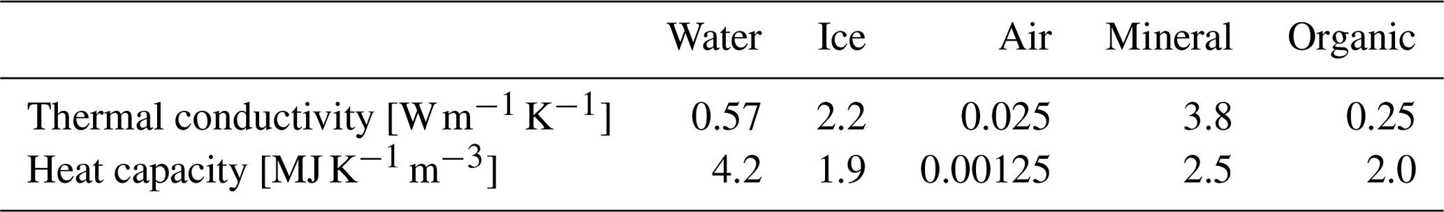
The bulk, temperature-dependent thermal conductivity k(T) is parameterized following (Cosenza et al., 2003) as the inverse quadratic mean of the constituents:

$$\begin{array}{}\text{(B5)}& \begin{array}{rl}k\left(T\right)=& (k_{\mathrm{w}}\cdot \sqrt{{\mathit{\theta }}_{\mathrm{w}}\left(T\right)}+k_i\cdot \sqrt{{\mathit{\theta }}_i\left(T\right)}+k_{\mathrm{a}}\cdot \sqrt{{\mathit{\theta }}_{\mathrm{a}}}\\ & +k_{\mathrm{m}}\cdot \sqrt{{\mathit{\theta }}_{\mathrm{m}}}+k_{\mathrm{o}}\cdot \sqrt{{\mathit{\theta }}_{\mathrm{o}}}{)}^{\mathrm{2}},\end{array}\end{array}$$

where k [$\mathrm{W}{\mathrm{m}}^{-\mathrm{1}}{\mathrm{K}}^{-\mathrm{1}}$] refers to the thermal conductivity of the constituent material. The bulk heat capacity is similarly computed as a simple weighted average:

$$\begin{array}{}\text{(B6)}& \begin{array}{rl}C\left(T\right)& ={\displaystyle \frac{\mathrm{1}}{\mathrm{5}}}(c_{\mathrm{w}}\cdot {\mathit{\theta }}_{\mathrm{w}}(T)+c_{\mathrm{i}}\cdot {\mathit{\theta }}_i(T)\\ & +c_{\mathrm{a}}\cdot {\mathit{\theta }}_{\mathrm{a}}+c_{\mathrm{m}}\cdot {\mathit{\theta }}_{\mathrm{m}}+c_{\mathrm{o}}\cdot {\mathit{\theta }}_{\mathrm{o}}),\end{array}\end{array}$$

where c values are the constituent heat capacities. Since we already vary the constituent fractions θ in our inversion procedure, we hold these values for the constituent thermal properties constant in all of our simulations. The values are shown in Table B5.

For time integration, we use an implementation of the second-order, explicit, strong-stability-preserving time stepping scheme of Shu and Osher (1988) provided by the Julia package, OrdinaryDiffEq.jl (Rackauckas and Nie, 2017). The time step size is set according to a suitable Courant–Friedrichs–Lewy (CFL) condition (Courant et al., 1967) for the nonlinear heat equation:

$$\begin{array}{}\text{(B7)}& \mathrm{d}{t}_{\text{max}}=\mathcal{C}\cdot \underset{i}{min}{\left[{\displaystyle \frac{\partial H}{\partial T}}\right]}_i{k}_i^{-\mathrm{1}}{\mathrm{\Delta }}_i^{\mathrm{2}},\end{array}$$

where ${\left[\frac{\partial H}{\partial T}\right]}_i$ [$\mathrm{J}{\mathrm{K}}^{-\mathrm{1}}{\mathrm{m}}^{-\mathrm{3}}$] is the apparent heat capacity at grid cell i, k_i [$\mathrm{W}{\mathrm{m}}^{-\mathrm{1}}{\mathrm{K}}^{-\mathrm{1}}$] is the thermal conductivity, Δ_i [m] is the vertical length of the grid cell, and $\mathcal{C}=\frac{\mathrm{1}}{\mathrm{2}}$ is the dimensionless Courant number which scales the step size to maintain stability.

B3 Inversion method

B3.1 Posterior predictions

From Eq. (7), the predictive distribution over the model states can be formulated as

$$\begin{array}{}\text{(B8)}& \begin{array}{rl}p\left({\mathit{x}}_{\mathrm{1}:\mathit{\tau }}\right|{\mathit{y}}_{\mathrm{1}:\mathit{\tau }},{\mathit{s}}_{\mathrm{1}:\mathit{\tau }})=& \underset{\mathit{\varphi }\in \mathrm{\Phi }}{\int }p\left({\mathit{x}}_{\mathrm{1}:\mathit{\tau }}\right|\mathit{\varphi },{\mathit{s}}_{\mathrm{1}:\mathit{\tau }})\\ & \times p\left(\mathit{\varphi }\right|{\mathit{y}}_{\mathrm{1}:\mathit{\tau }},{\mathit{s}}_{\mathrm{1}:\mathit{\tau }})d\mathit{\varphi },\end{array}\end{array}$$

with the process model $p\left({\mathit{x}}_{\mathrm{1}:\mathit{\tau }}\right|\mathit{\varphi },{\mathit{s}}_{\mathrm{1}:\mathit{\tau }})=\mathit{\delta }({\mathit{x}}_{\mathrm{1}:\mathit{\tau }}=f(\mathit{\varphi },{\mathit{s}}_{\mathrm{1}:\mathit{\tau }}))$, where f is the transient heat conduction model (described in Sect. 3.3) parameterized by ϕ, and δ is the Dirac delta distribution. Note that this formulation of the problem departs somewhat from typical data assimilation procedures which tend to focus more on probabilistic modeling of the state x, with parametric uncertainty in ϕ often neglected (Geer, 2021; Caers, 2018). In contrast, our approach amounts to a kind of “perfect model” assumption where the dynamics are assumed to be error-free. This allows us to avoid the need to develop a stochastic description of $p\left({\mathit{x}}_{\mathrm{1}:\mathit{\tau }}\right|\mathit{\varphi },{\mathit{s}}_{\mathrm{1}:\mathit{\tau }})$, while still being able to produce a distribution over plausible unobserved states via the parametric uncertainty induced by the prior. In principle, model error can be implicitly accounted for in the likelihood $p\left({\mathit{y}}_{\mathrm{1}:\mathit{\tau }}\right|{\mathit{x}}_{\mathrm{1}:\mathit{\tau }},\mathit{\varphi },{\mathit{s}}_{\mathrm{1}:\mathit{\tau }})$. However, as discussed in Sect. 5.5, EKS assumes the noise scale of the likelihood to be fixed and known a priori, which is generally insufficient for nontrivial inverse problems. As a result, the predictive distribution described by Eq. (B8) cannot be guaranteed to be well calibrated.

Estimating the predictive distribution in Eq. (B8) requires integration over the parameter space Φ weighted by the posterior distribution $p\left(\mathit{\varphi }\right|{\mathit{y}}_{\mathrm{1}:\mathit{\tau }},{\mathit{s}}_{\mathrm{1}:\mathit{\tau }})$ which is generally intractable. A Monte Carlo approximation to the integral can, however, be obtained by using sampling algorithms such as EKS to obtain samples from the posterior distribution.

B3.2 EKS problem setup

Since we aim to constrain the parameters ϕ of the heat conduction model f based on observed borehole temperatures, we choose g_T in Eq. (8) to be a simple aggregation function which computes mean annual ground temperatures (MAGTs) from the daily temperature profiles produced by f. For each site, we compute the modeled MAGT at each depth where a borehole sensor is present, linearly interpolating between grid cells where necessary. The resulting predicted temperatures form a matrix $T_{\text{pred}}=g_{\mathrm{T}}{}^{\circ }f\left(\mathit{\varphi }\right)\in {\mathbb{R}}^{N\times \stackrel{\mathrm{‾}}{d}}$, where N is the number of years and $\stackrel{\mathrm{‾}}{d}$ the number of borehole sensor depths at which data are available. Model outputs at all points in time and space where no data are present are thus not explicitly included in the likelihood calculation, though it is important to note that they are still included implicitly through conditional dependence of the evaluation points on the time dynamics of Eq. 3. We use the observed mean annual ground temperature from each borehole site as the observations, i.e., T_obs in Eq. (8), in the EKS algorithm. We specify the observation covariance Σ_T as a diagonal matrix with the posterior predictive variances obtained from our trend analysis (see Sects. 4.1 and B1) along the diagonal and a minimum variance of 0.01 K² (based on the temperature resolution of the thermistor chain, 0.1 K, according to manufacturer specifications). The diagonal structure of Σ_T assumes the observation noise to be both independent and uncorrelated across time and space.

The prior distribution over model parameters p(ϕ) is of crucial importance to any Bayesian inference procedure. Some parameters in the heat transfer model, such as soil composition, will cause the resulting optimization problem on ϕ to be under-constrained, since there may be more than one possible combination of soil components which have similar thermal properties. Additionally, incorporating prior knowledge about plausible parameter values allows us to reduce the amount of computational effort wasted on physically implausible or incoherent model configurations that may arise from random sampling. We define the priors for the heat transfer model parameters ϕ in their native, constrained parameter space Φ in order to more easily incorporate physically meaningful information about each site. More details on choices of priors for each site are in Appendix B3.3. We construct a diagonal, multivariate Gaussian approximation of our priors in the unconstrained parameter space via Laplace approximation of the density induced by γ(ψ). Note that this introduces some error into the EKS representation of the posterior, since the resulting Gaussian distribution is only an approximation of the transformed density.

B3.3 Selection of prior distributions

There are broadly three categories of parameters which are considered in our analysis: soil parameters (see Appendix B2.1), n factor parameters, and initial condition parameters. Separate soil parameters are defined for each stratigraphy layer. Soil freeze curve parameters (melting temperature T_m and van Genuchten parameters log α, log n) as well as porosity are varied in all layers, while organic content is only varied in the uppermost soil layer and is generally assumed to be zero or negligible in all other layers. Ground ice content is also varied only in layers where it is suspected to be present. Saturation of pore-space water and ice is varied as a single, global parameter used by each layer, excluding the bottom-most layer, which is held constant; since saturation is temporally constant throughout the simulation, this can be seen as effectively a bulk or average saturation level for the soil column.

We based the stratigraphy priors for Samoylov, Bayelva, and Barrow on previous modeling studies, Nitzbon et al. (2021), Zweigel et al. (2021), and Romanovsky and Osterkamp (2000), respectively. For Parson's Lake, we designed the stratigraphy based on the soil core analysis for the borehole site presented by Wolfe et al. (2010). We chose the priors for the van Genuchten parameters by fitting empirical freeze curves to temperature and volumetric water content measurements available for both the Samoylov Island and Bayelva sites (Boike et al., 2018a, 2019). The mean and standard deviation of the log-transformed parameters are set according to the fitted posterior statistics, with the variance increased by a factor of 100 to roughly account for uncertainty in extrapolation. We omit the details of this fitting procedure here for brevity, but the relevant code and results are included in the supplementary material. For Barrow, we used the same van Genuchten parameter priors derived from the 38 cm water content sensor at the Bayelva, since the freeze curve visually agreed with the one presented in Romanovsky and Osterkamp (2000), and both sites are known to have silty soil in the upper half meter (Boike et al., 2018a). We set these priors for Parson's Lake based on the reported soil types in each layer (Wolfe et al., 2010) using the Samoylov priors in the upper sandy layers and the Bayelva silty clay priors for the deeper layers. We stress that, in all cases, there is currently no systematic procedure used to derive the prior distributions; the process is largely based on subjective evaluation and iterative validation. Furthermore, the lack of stratigraphy information for the deeper layers is a substantial source of uncertainty in our analysis. While the variability induced by sampling from the prior distributions accounts for some of this uncertainty, there is a lot of room for improvement in the development of more rigorous and principled methods to derive prior distributions for soil stratigraphies and their corresponding parameterizations.