Widespread slowdown in thinning rates of West Antarctic ice shelves

Antarctica's floating ice shelves modulate discharge of grounded ice into the ocean by providing a backstress. Ice shelf thinning and grounding line retreat have reduced this backstress, driving rapid drawdown of key unstable areas of the Antarctic Ice Sheet, leading to sea-level rise. If ice shelf loss continues, it may initiate irreversible glacier retreat through the marine ice sheet instability. Identification of areas undergoing significant change requires knowledge of spatial and temporal patterns in recent ice shelf loss. We used 26 years (1992–2017) of satellite-derived Antarctic ice shelf thickness, flow, and basal melt rates to construct a time-dependent dataset of ice shelf thickness and basal melt on a 3 km grid every 3 months. We used a novel data fusion approach, state-of-the-art satellite-derived velocities, and a new surface mass balance model. Our data revealed an overall pattern of thinning all around Antarctica, with a thinning slowdown starting around 2008 widespread across the Amundsen, Bellingshausen, and Wilkes sectors. We attribute this slowdown partly to modulation in external ocean forcing, altered in West Antarctica by negative feedbacks between ice shelf thinning rates and grounded ice flow, and sub-ice-shelf cavity geometry and basal melting. In agreement with earlier studies, the highest rates of ice shelf thinning are found for those ice shelves located in the Amundsen and Bellingshausen sectors. Our study reveals that over the 1992–2017 observational period the Amundsen and Bellingshausen ice shelves experienced a slight reduction in rates of basal melting, suggesting that high rates of thinning are largely a response to changes in ocean conditions that predate our satellite altimetry record, with shorter-term variability only resulting in small deviations from the long-term trend. Our work demonstrates that causal inference drawn from ice shelf thinning and basal melt rates must take into account complex feedbacks between thinning and ice advection and between ice shelf draft and basal melt rates.

1 Introduction

The Antarctic Ice Sheet is Earth's largest reservoir of freshwater, with a global sea-level equivalent of ∼ 58 m (Morlighem et al., 2020). The rate at which Antarctica's ice is discharged to the ocean is controlled by its fringing ice shelves that exert a resistive “buttressing” force on the upstream grounded ice. In recent decades, ice shelves in West Antarctica's Amundsen Sea Embayment (ASE) have rapidly thinned (Paolo et al., 2015), and in response the grounded glaciers that feed them have accelerated (Mouginot et al., 2014; Konrad et al., 2017; Rignot et al., 2019; Gardner et al., 2018). There is some evidence that a similar drawdown and acceleration might also have started in some basins of East Antarctica (Roberts et al., 2018; Khazendar et al., 2013). This suggests that a reduction in buttressing may have already initiated a process of runaway retreat in regions that are inherently unstable due to the marine ice sheet instability (Weertman, 1974; Joughin et al., 2014; Rignot et al., 2014a). Thus, over the coming century the mechanisms that control ice shelf thickness change will be inextricably linked to global sea level, and improving our understanding of these processes will increase our ability to accurately predict Antarctica's overall contribution.

The processes that drive ice shelf thickness changes are directly linked to the atmosphere and ocean, and vary on different timescales (Paolo et al., 2018; Adusumilli et al., 2020). Ice shelves gain mass through the lateral influx of ice across the grounding line (the boundary where glaciers become afloat) and local surface accumulation via snowfall; mass is lost by calving, basal melt, and minor surface effects such as surface melting, wind scour, sublimation, and surface runoff. Ice shelf thickness can be estimated from satellite radar and laser altimetry, and previous studies have attributed observations of ice shelf thinning to increased rates of basal melting (Pritchard et al., 2012; Adusumilli et al., 2020); however, direct measurements of basal melt rates are scarce (Jacobs et al., 2013; Jenkins et al., 2018; Christianson et al., 2016; Dutrieux et al., 2014). Basal melt rates can be inferred from satellite-derived thickness fields combined with other inputs (ice divergence and surface mass balance), and previous large-scale melt-rate estimates made using this technique have considered mean rates for periods of less than a decade (Depoorter et al., 2013; Rignot et al., 2013), or have been limited in spatial resolution over longer time periods (Adusumilli et al., 2020). These data limitations have hindered our ability to identify the driving mechanisms and how basal melt rates vary with time.

In this paper, we combined observations from four satellite radar altimeters to derive a pan-Antarctic time series of ice shelf thickness and basal melt rates with the ability to resolve kilometer-scale structures (3 km grid at 3-month intervals) consistently from 1992 to 2017. In critical locations where significant ice thinning and flow acceleration have occurred, we corrected for time-variable ice divergence. Our dataset provides the most detailed picture of spatial and temporal changes in both ice thickness and basal melt rates, allowing us to disentangle the oceanic, atmospheric, and dynamic components of recent ice shelf change.

2 Data

2.1 Radar altimetry

We used data from four European Space Agency (ESA) satellite radar altimetry missions: ERS-1 (1991–1996), ERS-2 (1995–2003), Envisat (2002–2010), and CryoSat-2 (2010–2017). The first three satellites carried conventional pulse-limited altimeter systems with a footprint size of less than 3000 m in diameter over flat areas, sampling along flights every ∼ 370 m, with a latitudinal coverage up to 81.5^∘ S. CryoSat-2 (currently in operation) carries a dual antenna Doppler altimeter, operating in synthetic aperture radar interferometric (SARIn) mode over the margins of the ice sheet including the ice shelves, with a latitudinal coverage up to 88^∘ S. This altimeter yields along-track and across-track footprint sizes of about 300 and 3000 m, respectively, sampling along flight every ∼ 370 m. ERS-1 and ERS-2 operated in different modes of acquisition over the Antarctic ice shelves: “ocean mode” (330 MHz) with a finer sampling of the return radar echo, which translates to a higher-resolution radar waveform; and “ice mode” with a coarser sampling of the waveform (82.5 MHz), mostly to keep track of radar echoes interacting with terrain undulations on the ice sheet margins and interior.

We obtained ERS-1 and ERS-2 data from the “REprocessing of Altimeter Products for ERS (GDR): 1991 to 2003” (REAPER) (Brockley et al., 2017), as the product provides updated corrections and improved calibrations. We obtained Envisat data from the “RA-2 Geophysical Data Record” (GDR) v2 (https://earth.esa.int/eogateway/catalog, last access: 1 August 2023). We obtained CryoSat-2 data from “ESA L1b Baseline-C product” (Bouffard et al., 2018) using our own CryoSat-2 processor (Nilsson et al., 2016).

2.2 Firn and surface mass balance

Measured height changes reflect the (solid) ice thickness change and the changes in air content within the firn layer. To model the evolution of firn density (i.e., total column of firn air content, FAC) and surface mass balance (SMB), we used the Glacier Energy and Mass Balance model (GEMB) (Gardner et al., 2023). GEMB is run as a module of NASA's open-source Ice-sheet and Sea-level System Model (ISSM). It is a column model (no horizontal communication) of intermediate complexity, simulating thermal diffusion, shortwave subsurface penetration, meltwater retention, percolation and refreeze, effective snow grain size, dendricity, sphericity, and compaction. GEMB can accommodate the very long (thousands of years) spin-ups necessary for initializing deep firn columns.

2.3 Ice shelf boundary

Our ice shelf boundary definition is derived from a combination of Landsat imagery and ICESat data (Depoorter et al., 2013), updated for later epochs with the MEaSUREs v2 boundaries (Rignot et al., 2017) and manually edited for significant calving events from satellite imagery. Specifically for the Amundsen Sea sector, we constructed yearly boundaries from 1996 to 2018 at 240 m resolution.

2.4 Ice shelf velocity

We constructed a velocity product for the Amundsen Sea (time-varying) and Bellingshausen Sea (mean value) sectors by combining data from Mouginot et al. (2014) (1996–2012) and Gardner et al. (2018) (1985–2018) with complete coverage only after 2014. We synthesized multiple datasets to provide the best possible estimate of glacier surface velocity in a highly dynamic region of the ice sheet. The first dataset provides a long-localized record, while the second dataset provides pan-Antarctic coverage for later years. The first year with significant coverage is 1996 when InSAR ERS-1 data were collected over the ice sheet.

2.5 Sea surface height

We combined mean sea level directly measured with altimetry all the way to the ice shelf fronts through the sea-ice leads at 3 km resolution (Armitage et al., 2018), with the high-resolution gravity model GOCO05c (Fecher et al., 2017) to obtain the mean dynamic topography field. The geoid model combines modern gravity missions like GRACE and GOCE with in situ observations to provide unprecedented detail of the gravity field underneath the ice shelves. We also used sea-level trend data from CNES/AVISO (Guérou et al., 2023).

3 Methods

3.1 Ice shelf surface height

We derived surface heights from satellite radar altimeter return waveforms using the standard 30 % threshold retracker (ICE-1) available for all missions, except for CryoSat-2 where we used our in-house retracker for the SARIn mode (Nilsson et al., 2016). We then modeled and removed the static topography, applied a series of geophysical corrections, and modeled the firn air content and surface mass balance.

3.1.1 Topography removal

To measure the change in surface height, the static topography must be removed. We used a method similar to Nilsson et al. (2016), McMillan et al. (2014), and Wouters et al. (2015) but with some fundamental differences. In previous studies, the time-varying and static topography have been solved for in one least-squares inversion. This approach has an inherent limitation as generating time series of high temporal sampling requires a search radius of 1–3 km, which often does not allow for good estimation of the underlying topography that requires smaller spatial scales (<1 km). To this end, we first separated the data into ascending and descending orbits as well as into ice and ocean modes to mitigate the impact of any inter-mission and inter-mode biases. We treated ascending and descending orbits as independent datasets that we aggregated prior to the optimal interpolation stage (see Data fusion). We also filtered each ground track with a 3-point moving median to remove potential anomalous height measurements, e.g., from off pointing. We then solved for the static topography independently on each dataset using a biquadratic or bilinear surface model (depending on the number of available data points: biquadratic >30 pts > bilinear >15 pts > mean value >5 pts > NaN), which is removed to obtain the time-varying height-change signal. This approach allows us to accommodate the different spatial correlation lengths of the processes affecting the retrieval of height-change time series by permitting the use of independent search radii for the different steps included in the data processing workflow (e.g., 1 km radius for topography removal and 5 km radius for backscattering correction).

A key difference compared to previous studies (Paolo et al., 2015; Adusumilli et al., 2020) is that we set the inversion cells (i.e., search centroid and radii) following clusters of repeat tracks (along-track processing), leaving the gridding procedure for a later stage where we take into account the optimal spatial and temporal scales of each estimated quantity. Our inversion cell sizes vary linearly with latitude (8–15 km) to account for data density, decreasing with latitude as satellite ground track spacing becomes denser.

3.1.2 Grounding line and ice front

To avoid including grounded ice and ice front change signals in our analysis, we exclude all data within (i) a 3 km buffer around ice shelf perimeters, this is based on the pulse-limited footprint (∼ 3 km) of standard radar altimeters over flat areas, and (ii) an additional 3 km buffer (6 km total) from the ice shelf fronts to avoid errors resulting from changes in ice shelf boundaries (Greene et al., 2022).

3.1.3 Geophysical corrections

Various geophysical corrections are required for radar altimetry height data over ice shelves (Paolo et al., 2016). We describe the specific corrections we applied below.

• Standard corrections. We applied the dry troposphere, wet troposphere, ionosphere, solid earth tide, and pole tide corrections that are provided with the data.

• Surface slope. Because the radar altimeter echo is sensitive to terrain slope, reflecting off the point of closest approach (POCA) to the satellite, we relocated the observations to the POCA and corrected the range using the relocation method described in Bamber (1994) and based on the surface slope, aspect, and curvature information estimated from the Bedmap2 DEM (Fretwell et al., 2013).

• Inverse barometer. We calculated the inverse barometer correction using ERA-Interim mean sea-level pressure (Dee et al., 2011). Instead of the standard calculation that uses the global mean pressure over the ocean as the “reference pressure” (Le Traon et al., 1998), we used the climatological mean at each grid-cell location as our reference value, providing a spatially varying reference pressure field.

• Ocean tides. Ice shelves respond instantaneously to the rising and falling ocean tide, so this signal needs to be removed from the measured heights to retrieve freeboard height (height above sea level). We removed the original tide corrections that were applied to the raw height data and instead applied improved tides using the regional Circum-Antarctic Tidal Simulation model (CATS2008a), an updated version of the inverse tide model described by (Padman et al., 2002). This model has a higher resolution (∼ 4 km) and a more accurate land mask than global models, resulting in more accurate tide prediction close to the coast. We also corrected for the ocean tidal loading (the elastic deformation of the seabed in response to the ocean-tide load) using the TPXO7.2 model (Egbert and Erofeeva, 2002).

• Mean sea level and trend. Previous studies have estimated mean sea level (MSL) from low-order (i.e., low-resolution) geoid models and global mean dynamic topography (MDT) fields. Low-order geoid models contain substantial artifacts at the ocean–ice–land transition (Armitage et al., 2018), which introduces large biases to the estimated MSL underneath the ice shelves. Global MDT fields are usually extrapolated from the distant edge of the sea ice to the ice shelf grounding lines, as these global datasets do not contain measurements within the area covered by sea ice and ice shelves. This results in the propagation of incorrect ocean-state features underneath the ice shelves. Instead, we used MSL directly measured all the way to the ice shelf fronts (Armitage et al., 2018), removed the geoid (Fecher et al., 2017), extended the residual MDT with a Gaussian average tapering to zero at the grounding lines, and then added back the geoid. We extended the sea-level trend field in the same way.

• Surface scattering. The shape of the radar altimeter return waveform is governed by the degree of surface and volume scattering (Davis and Moore, 1993; Partington et al., 1989). Over the years many studies have used an empirical correction based on removing the correlation between changes in the observed height and changes in the shape of the radar waveform (Nilsson et al., 2016; Wingham et al., 2009; Zwally et al., 2005; Davis and Ferguson, 2004; Paolo et al., 2016). Here, we used estimates of the radar backscatter coefficient, leading edge width, and trailing edge slope (Rémy and Parouty, 2009; Khvorostovsky, 2012) to characterize changes in the shape of the radar waveform (Fig. 1). We normalized these parameters by their standard deviation and then regressed them, by means of robust multivariate regression (Holland and Welsch, 1977), against the residual time series of height changes (at the point-measurement level) to determine a linear combination of sensitivity gradients that we used to remove temporal changes in scattering effects from the original height time series. We note that the multivariate fit accounts for collinearity between the waveform parameters. We performed this procedure following the satellite ground tracks at intervals of 2 km with a search radius of 5 km, retaining the point within the search radius of the solution that has the highest sensitivity of any overlapping regressions (Nilsson et al., 2022). To reduce erroneous correlations to real elevation trends, we applied a difference operator to each parameter and to the height-change signal time series before the regression (Fig. 1).

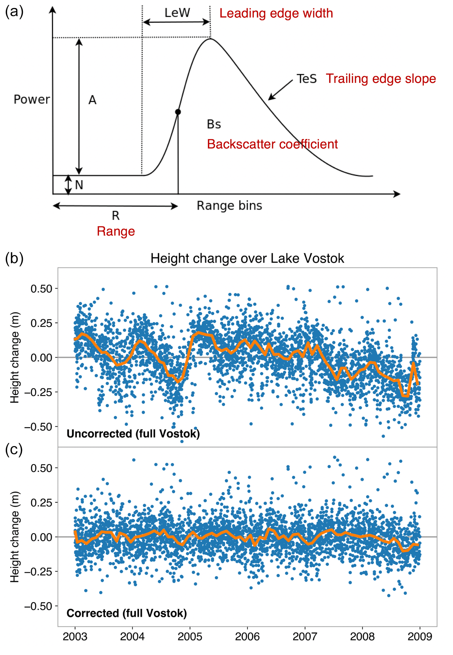
Figure 1 Multi-parameter radar scattering correction. (a) The different waveform parameters used to characterize the radar echo (where A is amplitude, N is the noise floor, and “Range bins” are the discrete samples of the return signal). (b) Time series of individual point high measurements before and after applying the scattering correction. The example shows Lake Vostok, where GPS records show near-zero surface height change (Richter et al., 2014).

3.1.4 Firn and surface mass balance calibration

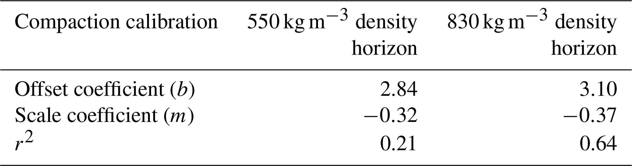
To produce the FAC and SMB used for this study (Schlegel and Gardner, 2022), we calibrate the GEMB model snow-densification parameters to improve the agreement between modeled snow-density profiles and observations after Ligtenberg et al. (2011) (Gardner et al., 2023). Calibration results for the ERA5 forcing simulations are summarized in Table 4. Following a relaxation simulation, as described by Gardner et al. (2023), the model is forced with 3-hourly ERA5 reanalysis for 1979–2017, resulting in daily spatial estimates of FAC and SMB. Results are converted to monthly estimates and then linearly interpolated onto a constant 5 km grid for ice shelf melt rate analysis and for the estimation of model uncertainties (Fig. 2).

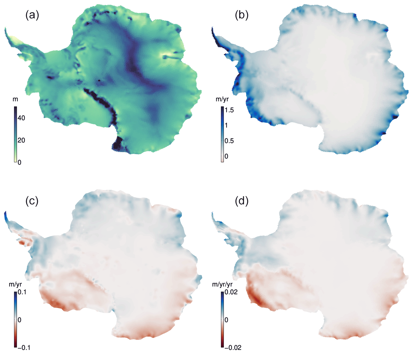
Figure 2 Glacier Energy and Mass Balance Model (GEMB). The 1992–2017 mean (a) firn air content (FAC) and (b) surface mass balance (SMB) simulated by GEMB forced with ERA5 reanalysis data, accompanied by the corresponding simulated trends in (c) FAC and (d) SMB over the same period.

3.2 Data fusion

We fused data from multiple satellites with different error characteristics and spatial distribution using an optimal interpolation approach (a.k.a. Gaussian processes). We used four key metrics to produce continuous fields at 3 km posting every 3 months: distance between observations, distance of observations to grid nodes (i.e., prediction points), observation errors, and along-track long-wavelength correlated errors (Melnichenko et al., 2014) that we estimated empirically so as to minimize the variance of the interpolated field. To determine the correlated errors, we first aggregated (binned) data from each individual mission in 5-month intervals at every 3 months (i.e., a sliding window overlapping by 1 month on each end). We then calculated empirical covariances as a function of data separation over the Ross Ice Shelf (constituting about $\mathrm{1}/\mathrm{3}$ of all ice shelf area), and fitted analytical covariance models that we used to guide the interpolation (Melnichenko et al., 2014). The covariances describing the characteristic correlation lengths are computed for each parameter (Fig. 3). We also used a latitude-dependent search radius to account for increased data density towards the pole as the satellite tracks converge (Fig. 4).

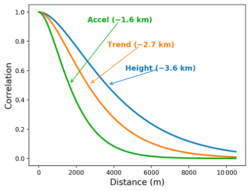
Figure 3 Decorrelation lengths for height, trend, and acceleration. Example of spatial correlation functions (or covariance normalized) used to derive continuous fields for each ice shelf parameter, without imposing a (single) spatial resolution a priori to all components. Shown in this example are typical spatial scales for each quantity derived from satellite radar altimetry (with dense and homogeneous coverage) over the Ross Ice Shelf, constituting about one-third of all surveyed ice shelf area.

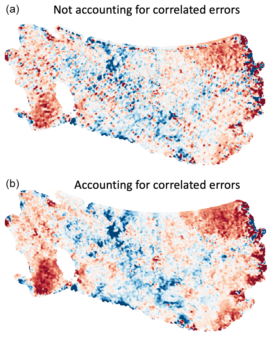
Figure 4 Optimal interpolation with correlated errors. Example of our spatial Optimal interpolation approach (one time step) where we account for the satellite along-track correlated errors. (a) Points along the same ground tracks share the same long-wavelength errors, producing a “track pattern” in the interpolated fields, which is the case in most standard interpolation approaches. (b) When correlated errors are accounted for (as off-diagonal elements in the error matrix), points sharing the same correlated errors are downweighed, producing a coherent spatial field. Example is north of 81.5^∘ S of the Ross Ice Shelf in Antarctica (approximately 800 km wide, horizontal scale in the figure).

At each grid cell, we then filtered and interpolated time series residuals larger than 5 standard deviations from the trend (defined by a piecewise polynomial fit). We also cross-calibrated the gridded records from the four satellite missions by computing the offsets (median of differences) between a low-pass-filtered version of the time series during the periods where consecutive missions overlapped. We filtered these records with a 5-point moving average (∼ 1.25 years) to remove the effect of seasonality.

3.3 Thickness change and basal melt rate inversion

We performed our melt estimation on an Eulerian reference frame. There are two fundamental steps that we improved upon previous work (Adusumilli et al., 2020, 2018; Paolo et al., 2018, 2016, 2015) to estimate ice shelf basal melting from measured surface height. First, inverting height to thickness

$$\begin{array}{rl}H\left(t\right)& ={\displaystyle \frac{{\mathit{\rho }}_{\mathrm{w}}}{{\mathit{\rho }}_{\mathrm{w}}-{\mathit{\rho }}_i}}\left(h_{\mathrm{0}}+\mathrm{\Delta }{h}_{\mathrm{altim}}+\mathrm{\Delta }{h}_{\mathrm{tide}}+\mathrm{\Delta }{h}_{\mathrm{load}}\right.\\ & \left.+\mathrm{\Delta }{h}_{\mathrm{IBE}}+\mathrm{\Delta }{h}_{\mathrm{FAC}}+\mathrm{\Delta }{h}_{\mathrm{MSL}}+\mathrm{\Delta }{h}_{\mathrm{SLT}}\right),\end{array}$$

where H is thickness, ρ_w and ρ_i are density of ocean water (1028 kg m⁻³) and ice (917 kg m⁻³), respectively, h₀ is mean surface topography from CryoSat-2 referenced to 2014, Δh_altim is height change from altimetry, and the respective corrections for tides (Δh_tide), load tide (Δh_load), inverse barometer effect (Δh_IBE), firn air content (Δh_FAC), mean sea level (Δh_MSL), and regional sea-level trends (Δh_SLT). Second, solving the mass balance equation

$$\dot{b}\left(t\right)={\displaystyle \frac{\partial H}{\partial t}}+\mathrm{\nabla }\cdot \left(H\mathit{u}\right)-\dot{a},$$

where $\dot{b}$ is total basal melt rate; $\partial H/\partial t$ is thickness change rate; ∇⋅(Hu) is ice-flux divergence, with $H=H_{\mathrm{0}}+H\left(t\right)$ and u being velocity; and $\dot{a}$ is surface accumulation rate (SMB). We note that all the terms in this equation are time dependent, with velocity varying in time for the Amundsen Sea sector only (Mouginot et al., 2014; Gardner et al., 2018) and assumed constant outside of this region due to lack of data. This assumption is justified by the relatively small flow changes observed outside of the Amundsen Sea sector in the past couple of decades (Gardner et al., 2018; Rignot et al., 2019). We computed our spatial and temporal derivatives implicitly, using a piecewise overlapping polynomial fit (Savitzky and Golay, 1964) that was designed to handle noisy data. We used a yearly fit window for temporal derivatives and a 15 × 15 km fit window for spatial derivatives.

3.4 Ice velocity fields

InSAR-derived velocities can contain substantial artifacts from ionospheric effects and residual tidal displacements. These artifacts are amplified by conventional (explicit) spatial derivatives and map onto the melt-rate estimates. Optical-derived velocities lack continental coverage and contain artifacts in places (Riel and Minchew, 2023). For this reason, we derive velocity fields by blending multiple products.

For the static (not changing in time) pan-Antarctic velocity field we merged the InSAR-based velocity of Mouginot et al. (2019), M19, and the optical-based time-aggregated velocity of Gardner et al. (2018, 2022), G18, following these steps that produced the best results determined through visual inspection:

1. M19 are mapped to the same 240 m grid as G18.

2. G18 was preferred everywhere that had a per-pixel observation count (i.e., number of velocity observations used to create time-averaged velocity) >100 or where M19 had no data. Using this criteria G18 and M19 account for 84 % and 16 % of data by area, respectively. The vast majority of M19 data are for latitudes >82.7^∘ S.

3. Velocities and errors were then combined using a 9-pixel (2160 m) cosine taper.

G18 and M19 velocities have an effective date of ∼ 2016 and ∼ 2012, receptively.

Use of a static velocity field is appropriate for the majority of the ice sheet where no observation of large temporal changes over the study period exist. For areas of rapid changes, i.e., the Amundsen Sea Sector of West Antarctica, we blended the annual resolved velocities of Gardner et al. (2018, 2022), G18, and Rignot et al. (2014b), R14. The annual velocity data have large errors and data gaps in both space and time that make the data challenging to work with. Considerable preprocessing is required to generate a blunder-free and continuous, in space and time, record of ice flow for the Amundsen Sea sector. These are the preprocessing steps that we applied.

1. R14 component velocities [v_x and v_y] are mapped to the same 240 m grid as G18 for the Amundsen Sea sector.

2. Velocities falling outside of mapped ice extents are set to no data values.

3. A reference velocity is defined as the 1996 velocity field or the earliest valid measurement thereafter. The average of both velocities is taken if multiple observations exist for the first year of data.

4. For areas moving faster than 200 m yr⁻¹, the percentage anomalies are calculated for all years relative to the reference velocity. This was done for both G18 and R14 velocities separately.

5. Annual velocity anomalies are then filtered with a 5 km windowed moving median.

6. G18 and R14 filtered anomalies are merged by taking the mean of each year. Years with less than 30 % coverage for fast-moving ice (≥200 m yr⁻¹) were discarded.

7. If missing annual values were within 25 km of a valid data point, they are filled using natural neighbor interpolation, otherwise anomalies were set to zero.

8. Outside of fast-moving areas, annual anomalies are tapered to zero using a 10 km cosine taper.

9. Merged and filled annual anomalies are then smoothed one last time using a 5 km windowed moving mean.

10. To create a continuous record of velocity, annual anomalies are interpolated in time to every $\mathrm{1}/\mathrm{5}$ of a year for every 240 m pixel using a spline interpolant and multiplied by the reference velocity.

11. Velocities are then smoothed, at the 240 m resolution, with a Gaussian kernel with standard deviation of 1.2 km prior to re-gridding onto our 3 km altimetry grid (Fig. 5).

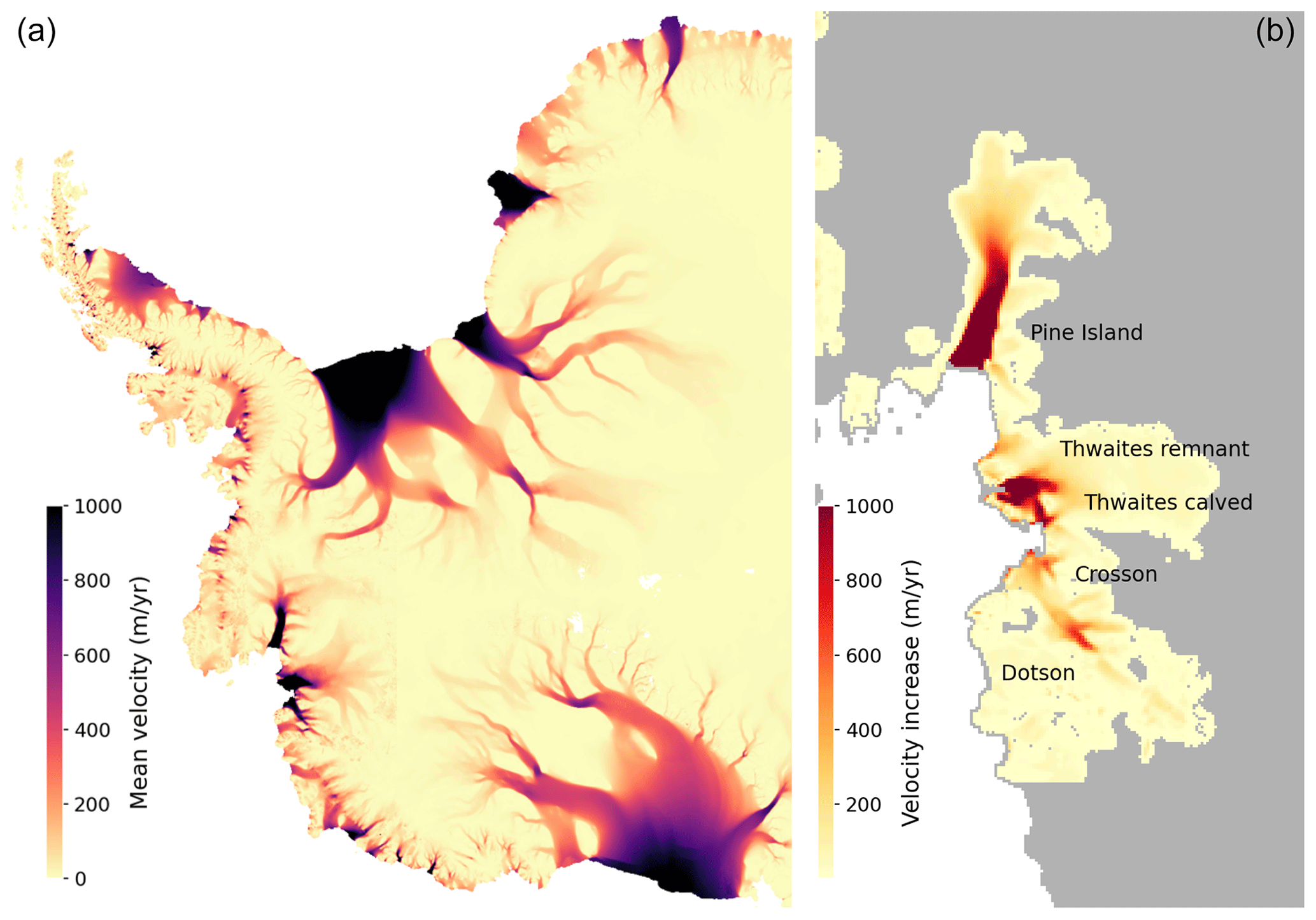
Figure 5 Mean ice shelf velocity and changes in Amundsen ice flow. Reference ice velocity (a) and velocity change from 1996 to 2017 (b; Gardner et al., 2022) used in this study. Ice shelves with velocity changes (from top to bottom): Pine Island, Thwaites remnant, Thwaites calved, Crosson, and Dotson.

3.5 Ice shelf thickness changes

The southern limit of ERS-1, ERS-2, and Envisat was 81.5^∘ S, so there is no data between 81.5 and 88^∘ S prior to the 2010 launch of CryoSat-2. To overcome this, we made the assumption that mean thickness and basal melt rates were constant prior to 2010 for areas >81.5^∘ S. This assumption is based on the insignificant changes (i.e., indistinguishable from noise given the variance in the data) in thickness and melting observed over those regions during the CryoSat-2 era.

We estimated acceleration or deceleration in ice shelf thinning from the trend in the thickness change rate time series. We fitted nonlinear trends using the Savitzky–Golay filter (Savitzky and Golay, 1964), which, unlike an ordinary least-squares line fit, is robust to outliers and sudden changes at the beginning and end of the records. Mean acceleration over the time span of our records is then defined as

$$\stackrel{\mathrm{‾}}{a}={\displaystyle \frac{\mathrm{\Delta }\stackrel{\mathrm{̃}}{\partial H}}{\mathrm{\Delta }t}},$$

where $\stackrel{\mathrm{̃}}{\partial H}$ is the mean rate of thickness change from the first versus last value of the trend fit, with Δt=26 years. Note that this is a robust estimate of acceleration (or second derivative) compared to the slope of a straight-line fit, as sudden changes in the trend are captured by our nonlinear trend fit. Finally, we compute the thickness change, basal melt, divergence, and SMB 2D mean fields from the mean of the respective instantaneous rate time series as

$$\stackrel{\mathrm{‾}}{\partial H}={\displaystyle \frac{\mathrm{1}}{n}}{\sum }_k\partial H_k,$$

where ∂H_k is the time-evolving rate of thickness change, and n is the number of samples in each grid cell record.

To analyze the temporal evolution of changes, we computed area-averaged time series of thickness for each ice shelf (excluding regions within 6 km of calving fronts or within 3 km of grounding lines) and compared to rates of elevation change from Nilsson et al. (2022) for neighboring locations upstream of the grounding lines (Fig. 11). To highlight the patterns over the deepest portion of the ice shelves and avoid any influence of advancing calving fronts, we show time series for the thickest 50 % ice of each ice shelf.

Our data of thickness change and basal-melt-rate estimates cover 53 ice shelves with a total area of about 1 541 700 km² (Table 3 and Fig. 16).

3.6 Ice–ocean modeling

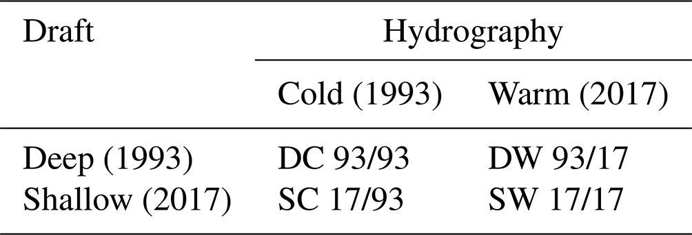
Observations of ocean properties relevant to ice shelf processes are sparse, making any inferences about changes in ocean forcing difficult to confirm. Thus, we use a simple “sandbox” experiment to assist the interpretation of the observed ice shelf changes. These simplistic model experiments are meant to (1) examine the influence of changes in ice shelf draft on basal melt rates in isolation of other environmental change and (2) test the ability of our thickness product to resolve basal melt structures. We run four model experiments: deep ice shelf draft subjected to cold ocean conditions (DC), deep ice shelf draft subjected warm ocean conditions (DW), shallow ice shelf draft subjected cold ocean conditions (SC), and shallow ice shelf draft subjected warm ocean conditions (SW). The year 1993 represents a year with a deeper draft (D) and colder ocean properties on the continental shelf (C), while the year 2017 represents a year with shallower draft (S) and warmer ocean properties (W) (Table 1).

Table 1 Model simulation abbreviations. The four model simulations are determined by the depth of the ice shelf draft (deep – 1993 and shallow – 2017) and the hydrographic properties on the continental shelf and in the ice shelf cavities (cold – 1993 and warm – 2017).

To model these conditions we use the Massachusetts Institute of Technology general circulation model (MITgcm) that includes a thermodynamic sea-ice model (Losch et al., 2010). Freezing and melting processes in the sub-ice-shelf cavity are represented by the three-equation thermodynamics of Hellmer and Olbers (1989) with modifications by Jenkins et al. (2001), as implemented in MITgcm by Losch (2008).

The model domain (Fig. 6) is derived from the global configuration (LLC1080) used by the Estimating the Circulation and Climate of the Ocean (ECCO) project (Forget et al., 2015), with a nominal horizontal grid spacing of ∼ 3 km on the Antarctic continental shelf, comprising the region of the Amundsen Sea used in Schodlok et al. (2012). The vertical discretization is enhanced, compared with that used by the ECCO project, to 113 vertical levels of varying thickness in order to capture the deep part of the sub-ice-shelf cavities near the grounding line. The bathymetry is a blend of IBCSO (Arndt et al., 2013) outside the sub-ice-shelf cavities and BedMachine Antarctica elsewhere (Morlighem et al., 2020). We derived ice shelf draft, the key component of our modeling experiment, from our ice shelf thickness data. Initial conditions and boundary conditions for hydrography (T, S, u, v) and sea ice are derived from a coarse-resolution global state estimate (∼ 20 km horizontal grid spacing, LLC270) for the integration period 1992 to 2017. Due to the difference in resolution between the global integration and the ∼ 3 km model domain, a relaxation is applied to temperature and salinity at the boundaries (10 grid points into the model domain) to avoid artifacts such as wave energy radiating into the model interior, and five grid points for sea-ice variables. Surface forcing is also provided by the ECCO project. We have successfully applied similar configurations to study ice–ocean interactions on the cube sphere as well as the lat-lon-cap (LLC) grids (Khazendar et al., 2013; Nakayama et al., 2017, 2018).

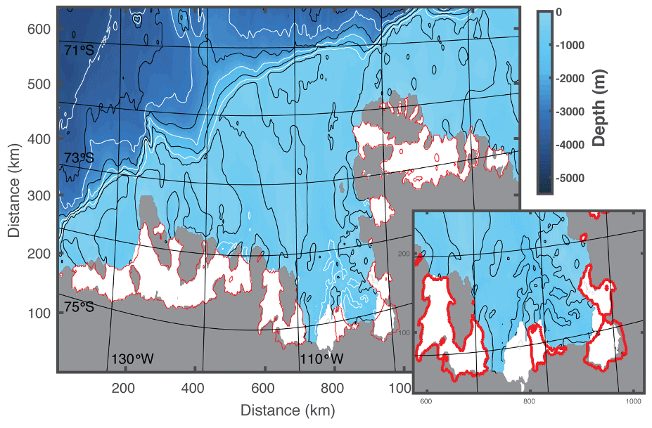
Figure 6 Amundsen Sea model domain at 3 km grid spacing. The Antarctic continent is depicted in grey, the ice shelf area for 1993 in white, and the ice shelf extent in 2017 in red contours. Contour lines of bathymetry from 500 m in 500 m intervals are shown in black, and from 1000 m in 1000 m intervals in white. Note the slight distortion of the LLC grid from a true latitude and longitude grid, ensuring little deviation from an isotropic grid. The inset shows the Pine Island, Thwaites, Crosson, and Dotson ice shelves, where grounding line and ice shelf front retreat is most prominent.

The model configuration comprises the ice shelf drafts and hydrography of the years 1993 and 2017. The year 1993 represents a year with a deeper draft and colder ocean properties on the continental shelf, while the year 2017 represents a year with shallower draft and warmer ocean properties. The initial integration starts from the LLC270 hydrography in 1992 (2016 respectively) for 1 year as a spin up. After the spin up, the surface forcing of the cold year 1993 (warm year 2017) is used as a repetitive forcing for 10 years of integration. The output of the last year of integration is averaged and its results analyzed. Additionally, we used the ice shelf draft of 1993 (2017) in the warm (cold) hydrography and surface forcing, and integrated for 10 years with the last year being averaged and analyzed. Thus, we have four model simulations: deep and cold, shallow and cold, deep and warm, shallow and warm (Table 1).

3.7 Uncertainty quantification

In situ basal-melt-rate measurements are not available at a large scale for Antarctica, and only a few localized (in time and space) indirect estimates exist. We therefore provide a formal statistical error by identifying and propagating the first-order uncertainties affecting our satellite estimates of ice shelf basal melt. Our uncertainties are based on quadratic propagation of the reported errors (e.g., from model outputs and velocities) and calculated standard deviations, adjusted for degrees of freedom.

Uncertainties in the GEMB FAC and SMB records are estimated by comparison to other firn models (GSFC FDMv1 (Smith et al., 2020; Medley et al., 2022) and IMAU FDM–RACMOv2.3 (Ligtenberg et al., 2014)) at the timescales of our melt-rate estimation (Fig. 3). At each grid node, we construct 5-month intervals of 5 daily (FAC) and monthly (SMB) rates, consistent with the 5-month sliding window we used to aggregate the altimetry data. We then calculate the standard deviation within the 5-month intervals and respective degrees of freedom (independent estimates) as a measure of model dispersion at different epochs (Fig. 4).

For each surface height grid cell, we estimated the 26-year variance of the height records, which is a conservative measure of error, as it accounts for both random fluctuations and geophysical signals. This error therefore reflects the complexity of local topography and our ability to model it, any residual tide and backscatter variability not fully accounted for, cross-calibration errors, and inherent variability such as seasonality. We then have

$$\begin{array}{c}{\displaystyle }{e}_h={\displaystyle \frac{\mathrm{1}}{\sqrt{n}}}\mathrm{SD}\left(h-h_{\mathrm{trend}}\right),\\ {\displaystyle }{e}_H={\displaystyle \frac{{\mathit{\rho }}_{\mathrm{w}}}{{\mathit{\rho }}_{\mathrm{w}}-{\mathit{\rho }}_i}}\sqrt{e_h^{\mathrm{2}}+e_{\mathrm{FAC}}^{\mathrm{2}}},\end{array}$$

where h is the height time series comprised of six independent datasets (four missions and two modes of operation), so we set n=6; h_trend is the trend from a piecewise polynomial fit; e_H is thickness error; e_FAC is the modeled firn air content error; and ρ_w and ρ_i are the densities of ocean water (1028 kg m⁻³) and solid ice (917 kg m⁻³), respectively.

Assuming no significant error (relative to other variables) in the timestamps, the spatial coordinates, and the 26-year mean thickness, and assuming the same error in both velocity components (u and v) of 5 m yr⁻¹ (see below), we then have

$$\begin{array}{c}{\displaystyle }{e}_{\partial H}={\displaystyle \frac{\mathrm{1}}{\mathrm{d}t}}\sqrt{e_{H_k}^{\mathrm{2}}+e_{H_{k+\mathrm{1}}}^{\mathrm{2}}},\\ {\displaystyle }{e}_{\mathrm{\nabla }}={\displaystyle \frac{\mathrm{1}}{\mathrm{d}x}}\mathrm{2}H{e}_u,\\ {\displaystyle }{e}_{\mathrm{melt}}=\sqrt{e_{\partial H}^{\mathrm{2}}+e_{\mathrm{\nabla }}^{\mathrm{2}}+e_{\mathrm{SMB}}^{\mathrm{2}}},\end{array}$$

where e_∂H is the error in the thickness change rate, e_∇ is the error in the ice-flux divergence, e_u is the error in the velocity fields, e_melt is the error in the basal melt rate, e_SMB is the error in the modeled surface mass balance, with $\mathrm{d}t=k=\mathrm{1}$ year (the time window used to estimate derivatives with a piecewise fit) and dx=3 km (the grid spacing).

For the mean rate of change fields, we take the variance of the respective instantaneous rate-of-change records. Here, again, our error estimate is conservative, as we are including natural variability as well as systematic trend changes, in addition to random errors, to the overall uncertainty. We then have the following error for the thickness change mean field:

$$e_{\stackrel{\mathrm{‾}}{\partial H}}={\displaystyle \frac{\mathrm{1}}{\sqrt{n/s}}}\mathrm{SD}(\partial H/\partial t),$$

where $\partial H/\partial t$ is the rate of thickness change time series, n is the number of samples, and s is a scaling factor to adjust the degrees of freedom for spatial correlation: $s=L^{\mathrm{2}}/A$, with L being the spatial scale of the variable in question and A our grid-cell area (∼ 9 km²). The same expression is used for divergence and SMB. We set L=3 km for thickness change rate (see Fig. 3 for typical decorrelation lengths over the ice shelves) and L=31 km for the smoother divergence and SMB fields (which corresponds to the grid resolution of the ERA5 reanalysis). The mean basal melt error is then obtained from a quadratic sum of these three errors.

Given that the acceleration term is derived from the end points of a trend fit to the instantaneous rate of change in thickness, its error can be estimated by

$$e_{\stackrel{\mathrm{‾}}{\mathrm{accel}}}={\displaystyle \frac{\sqrt{\mathrm{2}}}{\mathrm{d}t}}{e}_{\stackrel{\mathrm{‾}}{\partial H}}.$$

Then the errors for the ice shelf average values are simply the aggregate of the errors over each ice shelf (for thickness change, divergence, SMB, and acceleration)

$$\langle e_{\partial H}\rangle ={\displaystyle \frac{\mathrm{1}}{n}}{\sum }_i{e}_{{\stackrel{\mathrm{‾}}{\partial H}}_i},$$

with

$$\langle e_{\mathrm{melt}}\rangle =\sqrt{\langle e_{\partial H}{\rangle }^{\mathrm{2}}+\langle e_{▿}{\rangle }^{\mathrm{2}}+\langle e_{\mathrm{SMB}}{\rangle }^{\mathrm{2}}}.$$

3.8 Quality assessment

As an additional check on out results, we conducted a separate ice shelf mass budget calculation and compared to our explicitly calculated basal melt rates as well as the published melt estimates (Adusumilli et al., 2020). We do this by implicitly calculating melt rates using a control volume approach:

$${\displaystyle \frac{\partial M}{\partial t}}={\stackrel{\mathrm{‾}}{Q}}_{\mathrm{in}}-{\stackrel{\mathrm{‾}}{Q}}_{\mathrm{out}}+\stackrel{\mathrm{‾}}{a}-\stackrel{\mathrm{‾}}{b},$$

where $\partial M/\partial t$ is change in ice shelf mass, ${\stackrel{\mathrm{‾}}{Q}}_{\mathrm{in}}$ and ${\stackrel{\mathrm{‾}}{Q}}_{\mathrm{out}}$ are time-averaged (2010–2017) rates of ice fluxes across the grounding line and ice front (calving), respectively, $\stackrel{\mathrm{‾}}{a}$ is the time-averaged rate of surface accumulation (SMB), and $\stackrel{\mathrm{‾}}{b}$ is the time averaged basal melt rate for the period 2010–2017.

To calculate ice shelf mass balances, we define a control volume for each ice shelf, starting with the ice shelf outlines provided by (Mouginot et al., 2017). We adjusted the control volume outlines to remove any grid cells that are reported to have zero ice thickness data in BedMachine version 2 are missing surface velocity data in the ITS_LIVE static pan-Antarctic velocity field (Gardner et al., 2018) or do not have valid melt data in our estimates of mean melt rate for the 2010–2017 period. We then buffered the remaining outlines inward by 3 km on all sides of each ice shelf to avoid uncertain ice thickness estimates near grounding lines and to ensure confidence in ice-flux interpolation near dynamic calving fronts.

We also avoid complications that could be introduced by poorly understood effects of how bridging stresses might affect how basal melt anomalies get transmitted as expressions of surface elevation change. With this in mind, we considered only grid cells that are near hydrostatic equilibrium, which we identified using a simple ice flexure model with a threshold defined by bedmachine_interp(“flex”, x, y) >0.9 from Greene et al. (2017). If multiple, unconnected sections of control volume result for any ice shelf after adjusting the outlines, we use only the largest section for each ice shelf. As a final step, we interpolate to a consistent 100 m spacing along the outline of the control volume.

An example control volume is shown in Fig. 7. We note that by neglecting a buffered area around the perimeter of each ice shelf, the control volumes underrepresent the full extent of each ice shelf by 3 km on all sides, but our analysis is fully self-consistent, and we do not directly compare our mass balance estimates to previously published estimates that have been calculated for different control volumes.

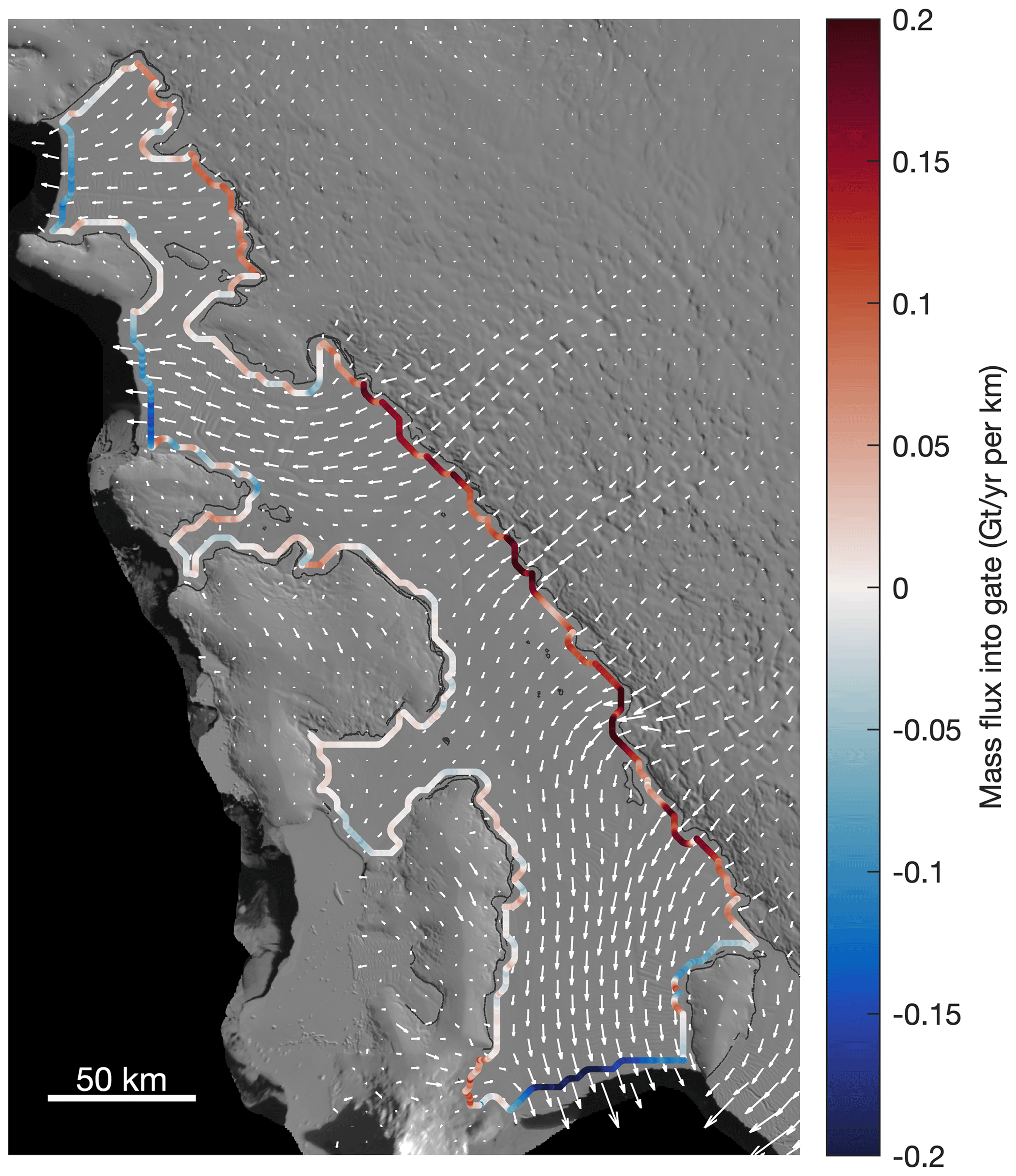
Figure 7 Control volume delineation for Getz Ice Shelf. Example of ice flowing into (red) and out of (blue) a control volume. For each ice shelf, we define a control volume as the largest hydrostatically floating area within previously published ice shelf outlines (Mouginot et al., 2017), which we buffer inward by 3 km. In this figure, white vectors show ice velocity from ITS_LIVE data and thin black lines show grounding lines compiled from InSAR measurements taken from 1994 to 2009 (Rignot et al., 2011).

To calculate ice flux into and out of each control volume, we interpolated surface velocity across the control volume flux gate using itslive_interp(“across”, x, y) in MATLAB (Greene et al., 2017), with any missing data filled with velocity estimates from Rignot et al. (2017). Ice flux at each point along the control volume is calculated as the product of ice thickness and ice velocity across the flux gate. For ice thickness we used our mean measurement of ice thickness for the study period. We also repeated the analysis using ice thickness from BedMachine version 2 but found no significant difference. The total ${\stackrel{\mathrm{‾}}{Q}}_{\mathrm{in}}-{\stackrel{\mathrm{‾}}{Q}}_{\mathrm{out}}$ mass balance for each ice shelf is calculated as the sum of the unit ice flux (flux per meter) measured along the control volume outline, multiplied by the 100 m spacing of our flux gate, and multiplied by ice density (917 kg m⁻³) to convert volume to mass.

To account for ice mass gained or lost at the surface ($\stackrel{\mathrm{‾}}{a}$), we converted GEMB mass balance outputs into units of Gt yr⁻¹ per grid cell, then calculated the sum of the SMB values for all grid cells within the control volume.

For our $\stackrel{\mathrm{‾}}{b}$, we generated a mean melt-rate map for the years 2010–2017 (the CryoSat-2 period), resampled it to 500 m resolution, then converted the map into units of Gt yr⁻¹ for each grid cell. The basal mass balance for every ice shelf is then obtained as the simple sum of the $\stackrel{\mathrm{‾}}{b}$ grid cells within the control volume outline of each ice shelf. For comparison to previous studies, we follow the same procedure to calculate total basal melt for each ice shelf using Adusumilli et al.'s (2020) 500 m resolution composite melt-rate map that spans 2010–2018. We used the provided w_b_interp field to fill in the missing grid cells, which they obtained by assigning melt rate based on a melt–depth relationship for each ice shelf.

4 Results

We first compared our basal-melt-rate estimates with those published by Adusumilli et al. (2020) and the basal melt rates that would be expected from two different control volume approaches (Fig. 8). In panels (a) and (b), we assumed that the volume of each ice shelf remained constant over the observation period, i.e., $\partial M/\partial t=\mathrm{0}$. In reality, most ice shelves experienced some change in thickness, which we accounted for in panels (c) and (d) by summing up the grid cells of a map of the linear trend in ice thickness that we generated from our data. In the flux gate calculation, we did not account for changes in velocity, but nonetheless, panel (d) shows good agreement between our estimated melt rates and the melt rates that would be expected from the control volume approach (as quantified in Fig. 8).

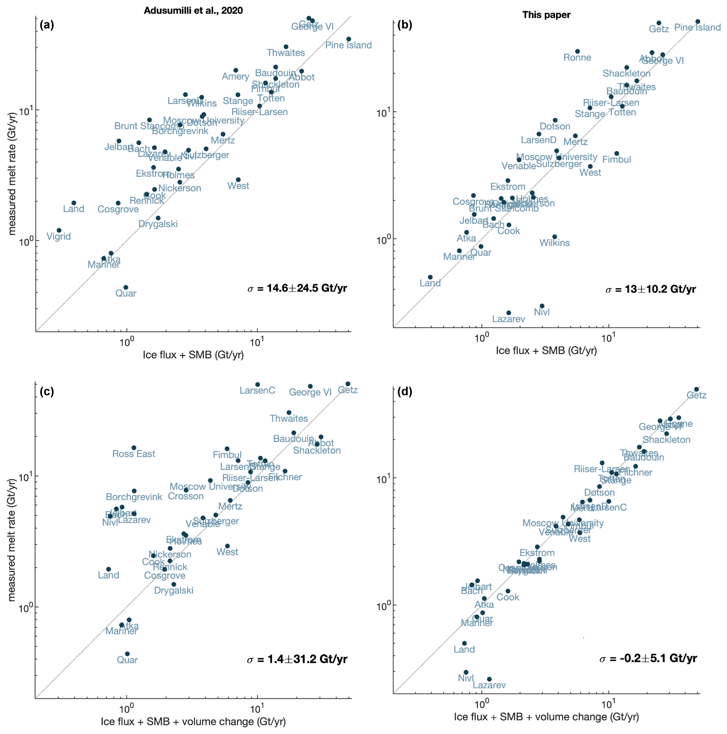
Figure 8 Comparison of estimates from this study with previous work. Comparison of (a, c) Adusumilli et al. (2020) and (b, d) this study's ice shelf basal melt estimates against a control-volume calculation of ice shelf mass change (line). The control volume is based on the input and output fluxes across the grounding line and ice front, mass gained or lost due to surface mass balance (a, b), and ice loss due to anomalies in basal melt (c, d). For this comparison, we only considered grid cells that are at least 90 % hydrostatically compensated (near fully floating).

Table 2 Contributions to change in thinning rate for major Amundsen Sea-ice shelves (1992–2008 to 2009–2017). Percentage contributions to the observed change in ice shelf thinning rate (Thin) from ice-flux divergence (Div), which includes ice advection, stretching (dynamic thinning) and surface mass balance (SMB). Units are meters of ice equivalent per year (m yr⁻¹). Only ice shelves with consistent availability of time-evolving velocity (needed to estimate time-evolving divergence) are shown. These quantities depict the change in the mean values from 1992–2008 to 2009–2017, averaged over the respective ice shelf areas. Note that if the averaging area is restricted to the thickest ice (i.e., areas close to the grounding lines), the contribution from basal melting is significantly larger (see Figs. 2 and 3).

Our pan-Antarctic analysis reveals spatial patterns of ice shelf thickness change (Fig. 9) that show the signature of ocean-induced melting, with the highest thinning rates found adjacent to the deep grounding lines (Fig. 10), where dense and warm modified Circumpolar Deep Water (mCDW) is more likely to be present and the pressure-melting point of ice is depressed. This overall pattern of ice shelf loss is consistent with previous estimates of ice shelf thinning (Paolo et al., 2015; Adusumilli et al., 2020; Shepherd et al., 2018); ice shelves in the ASE and Bellingshausen Sea Embayment (BSE) sectors, where the highest losses from the grounded ice are occurring, have all thinned over the past quarter century (Figs. 11 and 12). Our estimates for average ice shelf thinning rates in the ASE and BSE over the 1992–2017 observational period are 2.6 ± 0.3 and 0.5 ± 0.2 m yr⁻¹, respectively. The rate of change is relatively constant over the full period of study, suggesting that these ice shelves are largely responding to a change in ocean conditions that predates our satellite altimetry record, with shorter-term variability only resulting in small deviations from the long-term trend (Jenkins et al., 2018). The origin of the persistent long-term forcing is unknown; one plausible explanation is that changes in Antarctic zonal winds have enhanced the influxes of warmer waters underneath the ice shelves (Buizert et al., 2018), a phenomenon that has been linked to anthropogenic warming and teleconnections with tropical Pacific variability (Dutrieux et al., 2014; Sadai et al., 2020; Paolo et al., 2018; Holland et al., 2019).

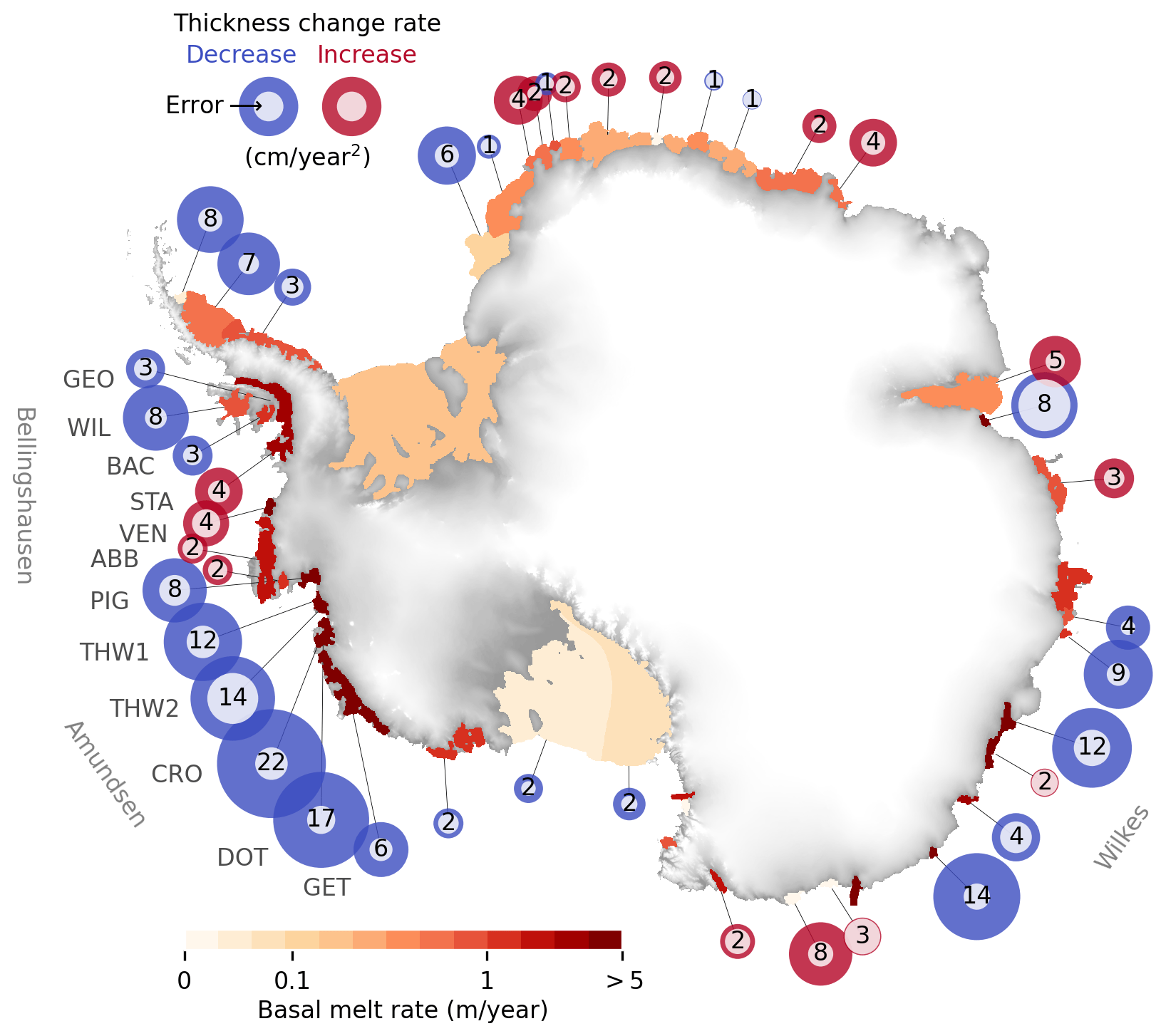
Figure 9 Ice shelf thinning has slowed where basal melt rates are highest. Circum-Antarctic pattern of acceleration or deceleration in ice shelf thickness change rate (circles) and basal melt rate (field) for each ice shelf. Blue circles represent a decrease, on average, in the rate of thickness change. Inner circles represent the respective uncertainties. Numbers depict thickness change rate values in cm yr⁻². All values are the 26-year means (1992–2017) averaged over the respective ice shelf areas (values near the grounding lines for the ASE in Fig. 14). Values are rounded for visualization purposes. Basal melt rates are displayed in logarithmic scale. Non-significant values are omitted from the plot.

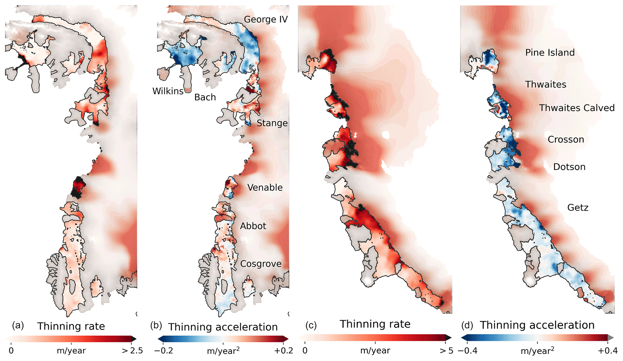
Figure 10 Slowdown in thinning is more pronounced where ice shelves are thicker. Panels (a) and (c): ice shelf and grounded ice thinning rate (in meters of ice equivalent per year); panels (b) and (d): mean acceleration (positive values, red) and deceleration (negative values, blue) in ice shelf and grounded ice thinning. Values are the mean over the 26-year period. The color bars depict ice shelf values; for reference, grounded ice values are an order of magnitude smaller than ice shelf values. The calved areas shown (e.g., Wilkins, Pine Island, and Thwaites ice shelf fronts) were excluded in all calculations.

All ice shelves in the Amundsen and Bellingshausen Sea sectors show dramatic rates of thinning since records began in the early 1990s, with thickness losses as high as 6.1 ± 0.5 m yr⁻¹ (Crosson) over the full ice shelf, confirming previous findings (Jenkins et al., 2018, 2010; Smith et al., 2017; Shepherd et al., 2004; Pritchard et al., 2012) that the dominant driver of change predates the satellite era. Over the 26-year record some ice shelves have thinned by more than 20 % near their original grounding lines, e.g., Thwaites 23 % (right before calving circa 2013), Crosson 35 %, and Dotson 25 % (Fig. 11).

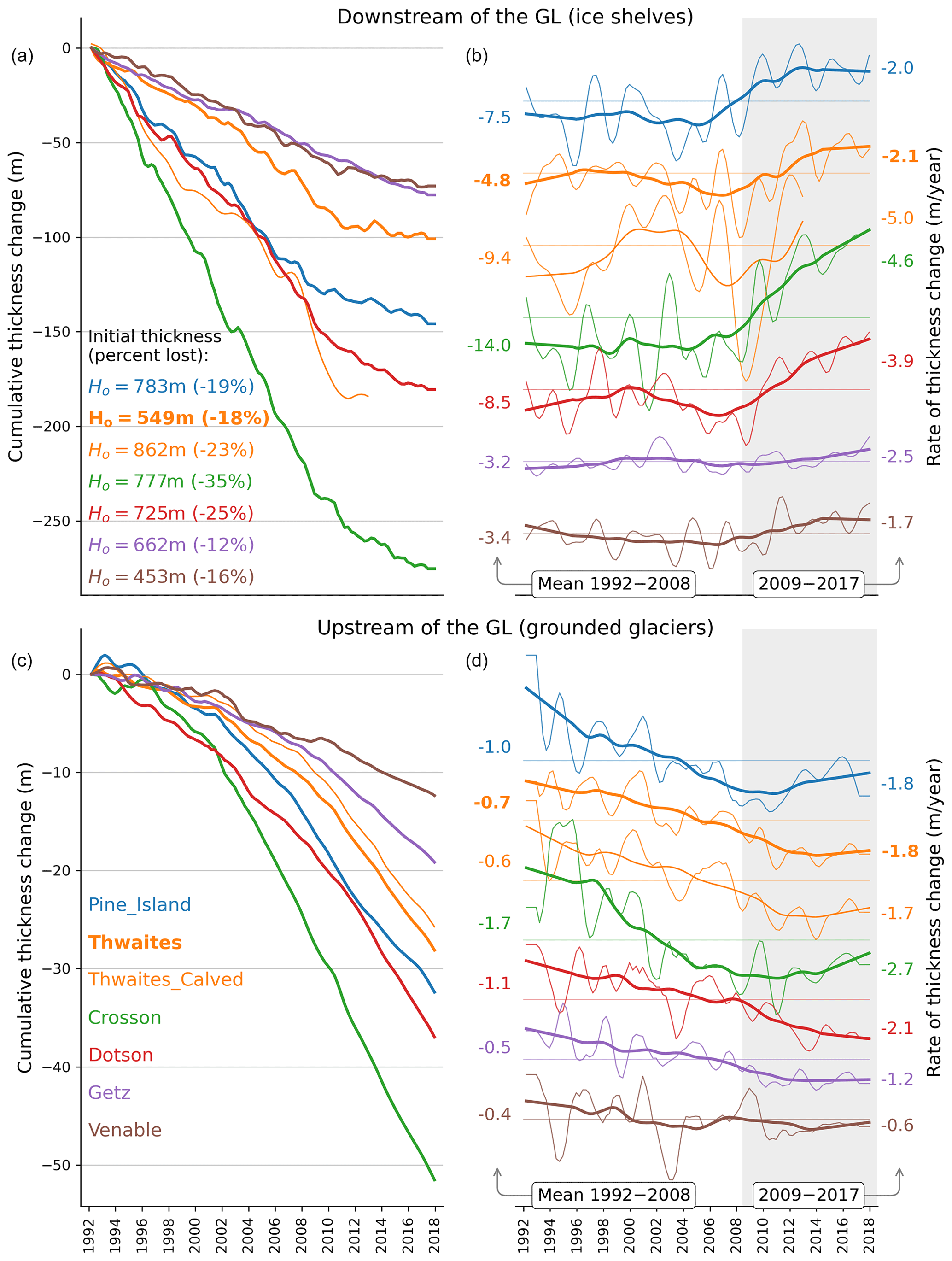
Figure 11 Thinning rates have slowed in the most recent decade across ice shelves. (a) Cumulative ice shelf thickness change for ice shelves with the highest losses in West Antarctica. (b) Respective rate of thickness change, with mean rate values for highlighted time intervals on each side (white/gray area). Ice shelf time series are averages over the area above the mean thickness value (i.e., the 50 % thickest ice). Unsmoothed time series with error bars and statistical significance of linear trends are shown in Fig. 12. (c, d) The same as the top panels but a few kilometers upstream of the grounding lines of the respective ice shelves.

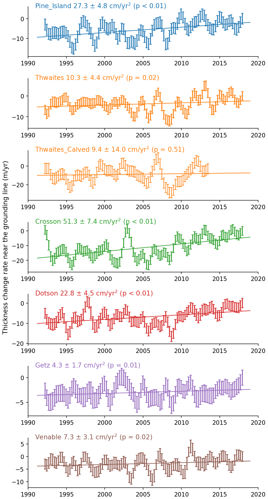
Figure 12 Time series of instantaneous rate of change in ice shelf thickness, unsmoothed with respective error bars, least-squares trend, and the associated statistical significance. A positive trend means deceleration in the thinning rate.

Our data reveal a large-scale coherent pattern of slowdown in rates of ice shelf thinning (Fig. 9) towards the end of the record, starting around 2008. The slowdown is most pronounced for those ice shelves that have thinned most over the 26-year period (Fig. 13) and is particularly accentuated along the West Antarctic margin where ocean melting of ice shelves is strongest (Fig. 10) but also occurs along Wilkes Land in East Antarctica. For the Amundsen Sea ice shelves, slowdown in thinning began between 2006 (Pine Island) and 2009 (Dotson), and at a later epoch in the Bellingshausen Sea sector (∼ 2010, Venable), somewhat consistent with previous single-ice-shelf studies (Jenkins et al., 2018; Davis et al., 2018). In many cases, the slowdown signal is sufficient to offset previous acceleration, with average deceleration reaching up to −22 ± 3 cm yr⁻² (or −51 ± 7 cm yr⁻² near the grounding line) for the Crosson Ice Shelf. Overall, we estimated an average thinning slowdown of 8.3 ± 1.3 and 1.1 ± 1.0 cm yr⁻² for the ASE and BSE, respectively.

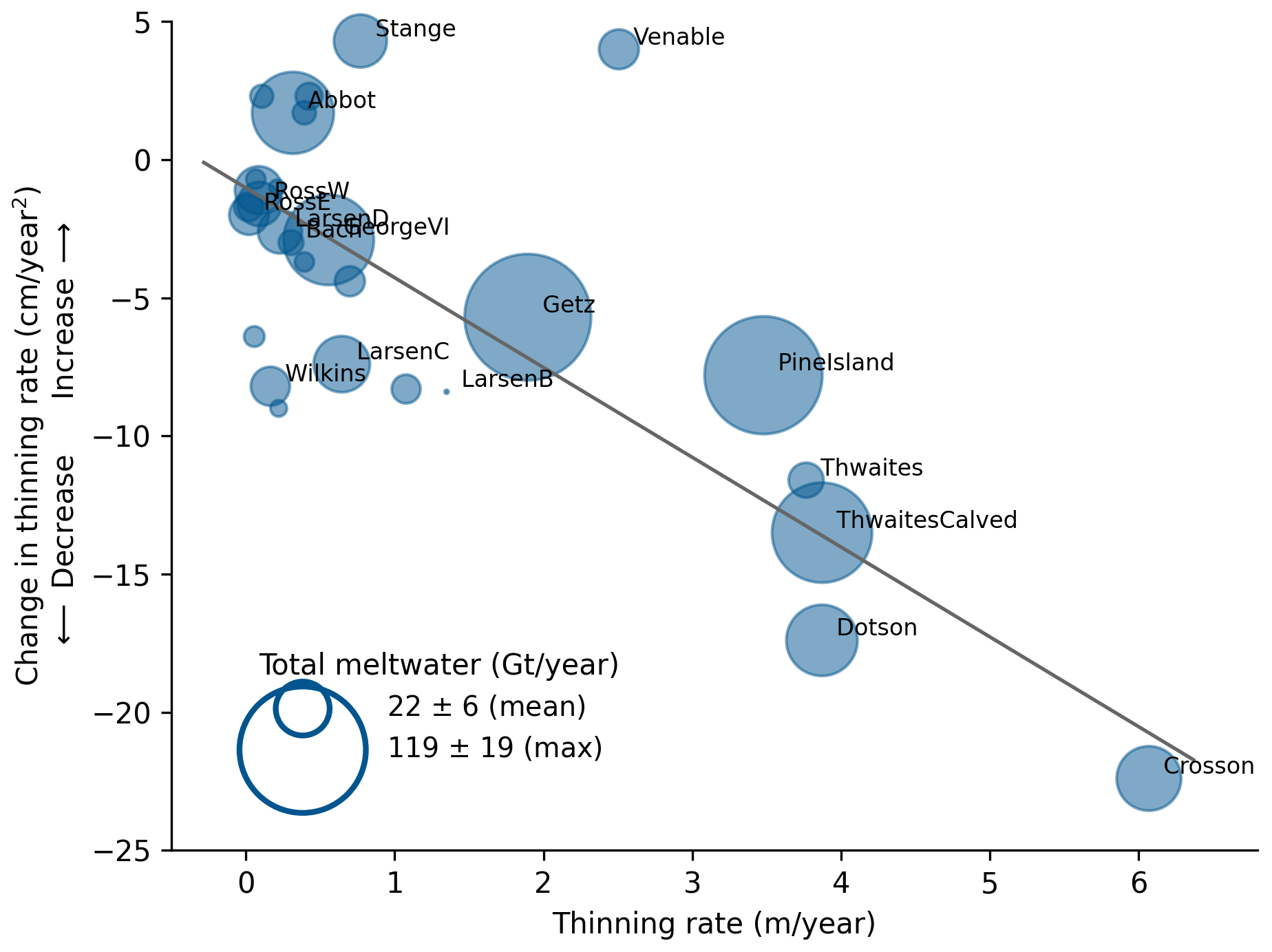
Figure 13 Thickness loss and slowdown in thinning are strongly correlated. Relationship between rates of ice shelf thinning and change in thinning rates around Antarctica. Only ice shelves with statistically significant acceleration (positive change) or deceleration (negative change) in thinning are displayed (30 ice shelves). Circle areas are proportional to the total meltwater produced (basal melt rate multiplied by ice shelf area), with Getz showing the largest value. The regression line has a correlation coefficient of $\mathit{\rho }=-\mathrm{0.74}$ ($\mathit{\rho }=-\mathrm{0.84}$ without Stange and Venable), with a p value <0.01 (all quantities with respective uncertainties are presented in Table 3).

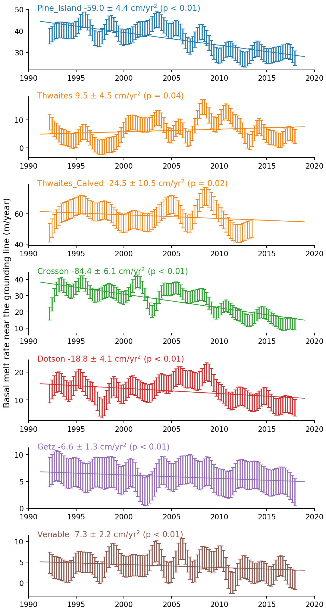
Figure 14 Basal melt rates have abated around the Amundsen Sea. Time series with error bars of basal melt rate (in meters of ice equivalent per year) for the thickest portions of the ice shelves, i.e., the area with thickness above the mean thickness value. Trend line (acceleration or deceleration) is a least-squares fit with respective statistical significance.

Our ice–ocean modeling result shows a highly resolved basal melt field (Fig. 15). When ocean forcing is held constant, melt rates for the 2017 geometry are generally lower than for the 1993 geometry near all grounding lines, with some localized patches of higher melt elsewhere on the ice shelves (Fig. 15). Modeled basal melt rates are 25 % to 50 % lower near the grounding lines of the Dotson and Crosson ice shelves when using the shallow (2017) ice shelf geometry compared to rates determined from the deeper (1993) geometry.

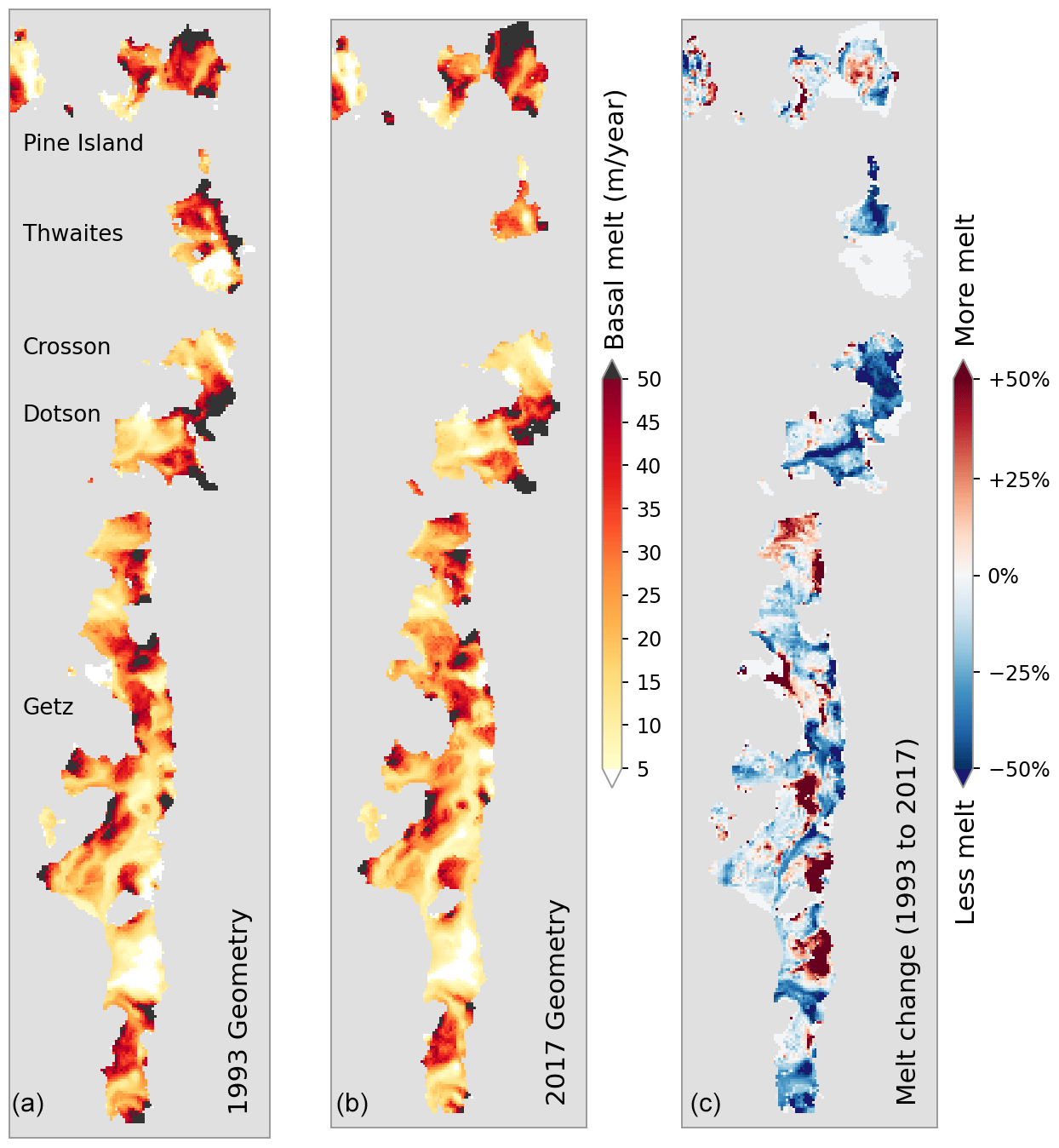
Figure 15 Satellite ice shelf thickness yields high-resolution modeled basal melt rates. Holding ocean temperatures constant at the “warm” conditions observed in 2017, modeled melt rates for ice shelf draft and front positions corresponding to 1993 (a) and 2017 (b) show an overall reduction in melt rates (c) resulting from changes in ice shelf geometry alone (See Table 1). Results using “cold” ocean conditions of 1993 show a similar pattern, suggesting that the effects from changing ice shelf geometry occur regardless of changes in ocean temperature. Insignificant melt-rate values (<0.1 m yr⁻¹) and non-overlapping areas between 1993 and 2017 are masked out (white).

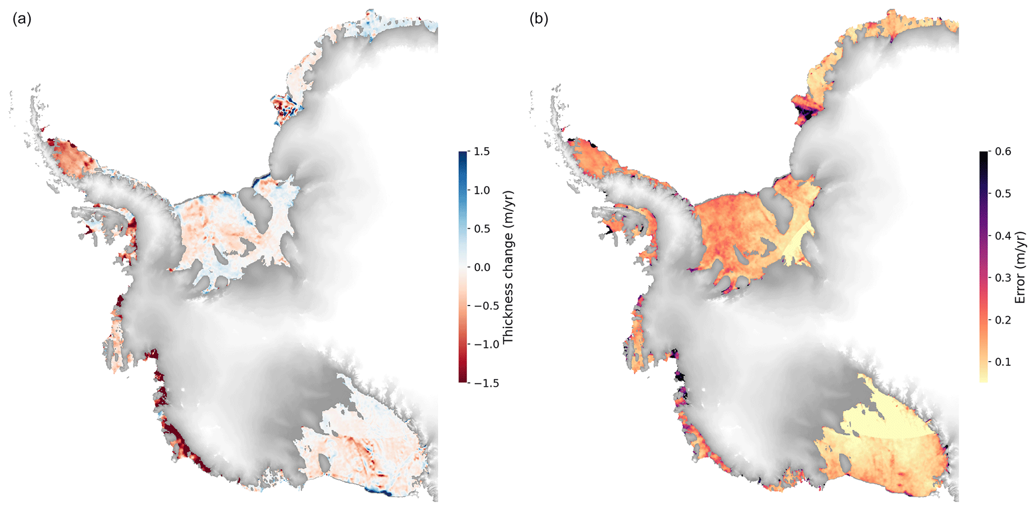
Figure 16 Satellite-derived thickness change field and associated error. Ice shelf thickness change rate (a) and associated error (b) from which basal melt rates are estimated.

5 Discussion

Thinning of grounded ice (Nilsson et al., 2022) between 3 and 12 km upstream of the grounding line (Fig. 11) shows that the grounded ice losses have increased on average in West Antarctica as a dynamical response of glacier flow to loss of ice shelf buttressing and grounding line retreat (Konrad et al., 2017; Gudmundsson et al., 2019; Milillo et al., 2022). More recently, however, the rate of grounded ice loss appears to be responding to the slowdown in the rate of ice shelf thinning, as suggested by the coincident change in the trend of both floating and grounded thickness change records (Fig. 11). Grounded ice flow is also controlled by factors other than ice shelf thickness (i.e., changes in ice shelf front, grounding line position, pinning points, and basal friction), and changes in ocean hydrographic properties may ultimately dictate how the ice sheet will change over the coming centuries. The longer-term response of glacier flow to the slowdown in ice shelf thinning in the region remains to be confirmed.

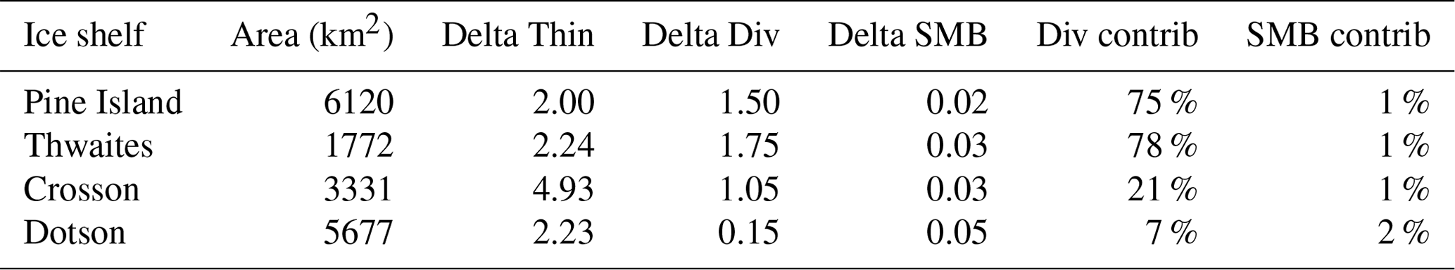
The slowdown in thinning rates implies a recent decrease in the rate of ice shelf mass loss. Satellite measurements of ice thickness alone cannot directly indicate whether the slowdown in thinning rates reflects an increase in grounded ice flux, an increase in surface accumulation, or a decrease in basal melt rates. We found that substantial changes in ice flow occurred on both the floating and grounded ice (Mouginot et al., 2014; Konrad et al., 2017; Gardner et al., 2018), with velocity increases over the ice shelves up to 4 times those of the grounded glaciers that feed them. A widespread ice flow acceleration across the grounding line in the Amundsen Sea sector after the 2000s (Mouginot et al., 2014) provided a sudden influx of ice, decreasing ice shelf thinning rates by over 1.5 m yr⁻¹, which accounted for about 75 % of the slowdown in the observed rate of ice shelf thinning in Pine Island and Thwaites. The dynamic contribution to thinning deceleration was less, but still substantial, in the case of Crosson (1.1 m yr⁻¹ or 21 %) and significantly less for Dotson (∼ 0.2 m yr⁻¹ or 7 %) (Table 2). Changes in ice flow alone are, therefore, unable to fully explain the observed slowdown in thinning rates. An investigation of changes in surface mass balance shows relatively minor trends in surface accumulation over the observation period (Fig. 2), with little impact on the overall rates of ice shelf thickness change (accounting for 1 %–2 %, Table 2), leaving changes in ocean melt rates as the most likely contributor to the remainder of the recent slowdown in thinning rates not accounted for by changes in ice flux.

Our results show that rates of ice shelf basal melt have systematically decreased near the grounding lines, by varying degrees, from the late 2000s to 2017. This reduction in basal melt is greatest in the regions of West Antarctica that have been changing most rapidly, such as the Pine Island, Thwaites, Crosson, Dotson, and Venable grounding lines (Fig. 14). These ice shelves are also the thickest, with their deep grounding lines exposed to intrusions of mCDW through bathymetric troughs, in contrast to shallower ice shelves in the region that do not exhibit a clear reduction in melt rate (e.g., Abbot and Cosgrove). The largest decreases in basal melt rate, over the 26-year period, are found near the grounding lines of the Pine Island and Crosson ice shelves, with −59 ± 4 and −84 ± 6 cm yr⁻², respectively. On some ice shelves, such as Venable and Stange, slowdown in thinning and basal melting is strictly confined to the floating ice near the grounding line (Fig. 10). For Venable, this results in a slight overall increase in thinning and melting, on average, for the full ice shelf extent (Fig. 9 and Table 3) but substantial decrease near the grounding line (within approximately 8 km): −7 ± 2 cm yr⁻² reduction in meltwater rate (Fig. 14). One factor limiting estimates of time-dependent basal melt rates is the lack of time-variable velocity information. In general, ice shelves outside the Amundsen sector have not experienced dramatic velocity changes (Rignot et al., 2019; Gardner et al., 2018). Assuming a constant velocity field, however, can bias (high) estimates of basal melt change of ice shelves, such as Getz, known to have had velocity increases in the order of 10–100 km yr⁻¹ along the grounding line, resulting in a 6 % increase in ice flux (Gardner et al., 2018; Selley et al., 2021). Still, modest velocity changes such as those observed on the Dotson Ice Shelf (Fig. 5) only contributed about 7 % to the total change in thinning rates (Table 2).

Table 3 Antarctic ice shelf change mean values (1992–2017). Thinning rate, basal melting, and thinning acceleration (in meters or centimeters of ice equivalent per year) are the 26-year mean values averaged over the respective ice shelf areas, excluding a 3 km buffer along the grounding lines and a 6 km buffer along the ice fronts. Area values shown (in squared kilometers) refer to total ice shelf area. Ice shelves smaller than 1 km² have been excluded due to the resolution limitation of the satellite altimeters.

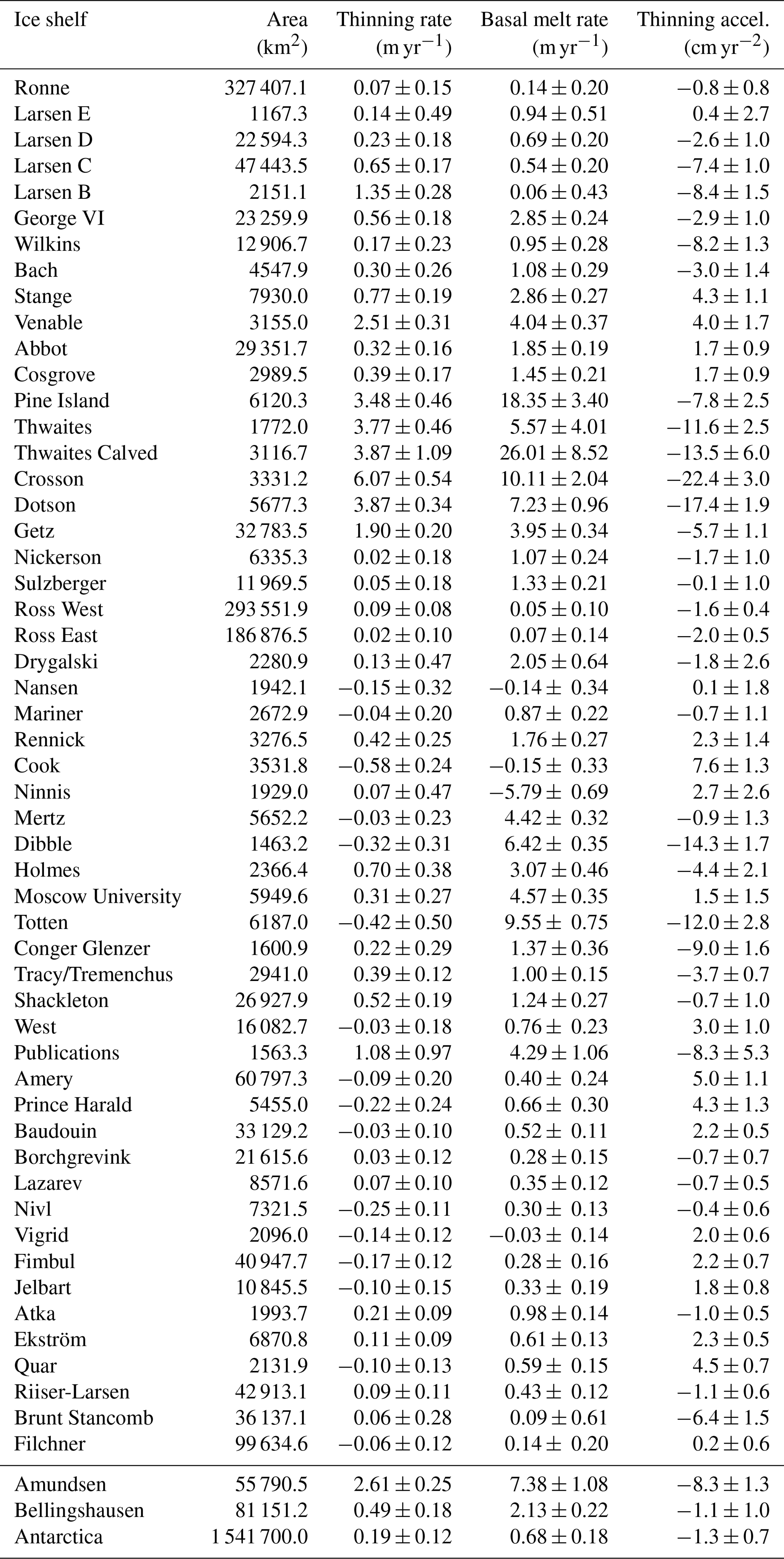
Table 4 Derived calibration offset and scale coefficients. Coefficients for firn compaction derived from calibration methods as described by Gardner et al. (2023), along with the correlation coefficient.

Ice shelf basal melt rates are sensitive to changes in the ice shelf draft depth, which dictates the temperature of the ocean waters that come into contact with the ice shelf base (Padman et al., 2012; Schodlok et al., 2012). A melt reduction at depth is, therefore, consistent with the notion that inflows of mCDW into the sub-ice-shelf cavities may be counteracted by a thinned ice shelf, whose draft sits in shallower (cooler) waters (Padman et al., 2012), or with the idea that cold meltwater from the deep grounding lines might reduce melt at shallower depths (Lewis and Perkin, 1986). Other investigations, however, have suggested that in the early 2010s ocean conditions in the ASE changed, further contributing to a reduction in basal melt of the West Antarctic ice shelves (Jenkins et al., 2018; Webber et al., 2017). We note that our modeling experiments do not negate the influence of changes in thermocline depth on ice shelf melt, or are intended to single out a driving mechanism (due to their simplicity), but rather suggest that changes in cavity geometry alone play a significant role in melt variability.

The link between ice shelf thinning and ice shelf melt comprises a negative feedback relationship that acts in tandem with a separate negative feedback relationship between grounded ice acceleration and ice shelf thinning: (i) prolonged ice shelf thinning and grounding line retreat have reduced the backstress that ice shelves provide, allowing outlet glaciers to accelerate (Konrad et al., 2017; Gudmundsson et al., 2019; Minchew et al., 2018), and the new influx of grounded ice has provided some mitigation to the overall thinning rate of ice shelves in the ASE and BSE. (ii) Thinning has most likely contributed to a reduction in basal melt rates by placing ice shelf drafts in cooler waters compared to their geometric configuration in the 1990s and early 2000s (Padman et al., 2012). We hypothesize that these two feedback mechanisms account for the majority of the recent slowdown in ice shelf thinning, with the remainder attributable to a multi-year reduction in basal melt due to a change in hydrographic properties (e.g., a temporary shift in the depth of the thermocline).

6 Conclusion

We have examined the time-varying evolution of Antarctic ice shelf thickness and ocean melt rates over a 26-year period. We show that overall thinning around Antarctica is consistent with previous studies but also that there has been a significant and consistent slowdown in rates of thinning since around 2008 across several West Antarctic and Wilkes basin ice shelves. Much of the slowdown in thinning can be attributed two key negative feedbacks: the thickness–flux feedback and the thickness–melt feedback. In the thickness–flux feedback, ice thinning leads to a reduction in the backstress exerted by the ice shelf on upstream grounded ice, which in turn leads to an increase in ice flux across the grounding line that reduces rates of ice shelf thinning. In the thickness–melt feedback, ice thinning results in a shallower ice shelf draft, exposing the ice shelf to waters with reduced heat content, leading to a reduction in melt rates. We hypothesize that the remaining unaccounted for reduction in basal melt rates point to a reduction in ocean forcing.

We note that our observations span only 26 years, and the reduction in thinning and basal melt that we report may represent a temporary adjustment period on decadal timescales. We neglect areas within 3 km of the grounding line to limit the influence of bridging stresses; yet, our measurements could still be influenced by local transient changes in the hydrostatic state of ice within our areas of observation. The melt rates we report could also be influenced by changes in grounding line position that occur outside our region of analysis, as hotspots of melt migrate nearer or farther from our fixed mask. Nonetheless, the slowdown in melt that we report is seen across several ice shelves, and in multiple sectors of Antarctica.

The above-mentioned feedbacks will be captured by fully coupled instantaneous response ice–ocean models (e.g., Goldberg et al., 2012; Seroussi et al., 2017). These models, however, are computationally expensive and not currently included in the pan-Antarctic ice sheet models that have been used to generate sea-level projections for the coming century (Seroussi et al., 2020; Fox-Kemper et al., 2021). We cannot offer a complete picture of the long-term impact of the processes we describe until they are adopted in fully coupled pan-Antarctic ice–ocean models. However, our findings indicate that by including ice dynamic feedbacks and the tendency for ice shelves to thin themselves into cooler waters, projections of ice loss may prove more complex and possibly more tempered than current estimates suggest.