Spatially continuous snow depth mapping by aeroplane photogrammetry for annual peak of winter from 2017 to 2021 in open areas

Information on snow depth and its spatial distribution is important for numerous applications, including natural hazard management, snow water equivalent estimation for hydropower, the study of the distribution and evolution of flora and fauna, and the validation of snow hydrological models. Due to its heterogeneity and complexity, specific remote sensing tools are required to accurately map the snow depth distribution in Alpine terrain. To cover large areas (>100 km²), airborne laser scanning (ALS) or aerial photogrammetry with large-format cameras is needed. While both systems require piloted aircraft for data acquisition, ALS is typically more expensive than photogrammetry but yields better results in forested terrain. While photogrammetry is slightly cheaper, it is limited due to its dependency on favourable acquisition conditions (weather, light conditions). In this study, we present photogrammetrically processed high-spatial-resolution (0.5 m) annual snow depth maps, recorded during the peak of winter over a 5-year period under different acquisition conditions over a study area around Davos, Switzerland. Compared to previously carried out studies, using the Vexcel UltraCam Eagle Mark 3 (M3) sensor improves the average ground sampling distance to 0.1 m at similar flight altitudes above ground. This allows for very detailed snow depth maps in open areas, calculated by subtracting a snow-off digital terrain model (DTM, acquired with ALS) from the snow-on digital surface models (DSMs) processed from the airborne imagery. Despite challenging acquisition conditions during the recording of the UltraCam images (clouds, shaded areas and fresh snow), 99 % of unforested areas were successfully photogrammetrically reconstructed. We applied masks (high vegetation, settlements, water, glaciers) to increase the reliability of the snow depth calculations. An extensive accuracy assessment was carried out using check points, the comparison to DSMs derived from unpiloted aerial systems and the comparison of snow-free DSM pixels to the ALS DTM. The results show a root mean square error of approximately 0.25 m for the UltraCam X and 0.15 m for the successor, the UltraCam Eagle M3. We developed a consistent and reliable photogrammetric workflow for accurate snow depth distribution mapping over large regions, capable of analysing snow distribution in complex terrain. This enables more detailed investigations on seasonal snow dynamics and can be used for numerous applications related to snow depth distribution, as well as serving as a ground reference for new modelling approaches and satellite-based snow depth mapping.

1 Introduction

Accurate snow depth mapping is important for the assessment, prediction and prevention of natural hazards such as snow avalanches or floods. Crack propagation and the size of release areas of snow avalanches are, for example, linked to snow depth distribution (Veitinger and Sovilla, 2016; Schweizer et al., 2003). The snow depth distribution and therefore avalanches are strongly influenced by wind-induced snow drift in the starting zone as well as the avalanche path (Schön et al., 2015). Further hazards related to snow depth are snow loads on buildings, threatening not only the stability of roofs but potentially leading to dangerous roof avalanches (Croce et al., 2018). Additionally, besides snow density assumptions, snow depth measurements are key to better assess the corresponding snow water equivalent (SWE). The available SWE is crucial for flood forecasting and the operation of hydropower (Magnusson et al., 2020). Spatially explicit information on snow depth distribution on and next to the pistes is also valuable for winter resorts and can be used to validate snow depth measurements captured by snow groomers (Spandre et al., 2017; Ebner et al., 2021). Moreover, snow depth mapping facilitates research on the interaction between snow depth distribution and flora and fauna (Wipf et al., 2009).

Precise snow depth measurements are key to validating models for snow parameters. In avalanche modelling tools such as the Rapid Mass Movement Simulation (RAMMS) (Christen et al., 2010), the snow volume derived from snow depth maps can be compared to modelled results. Furthermore, snow depth maps can serve as a reference for snow depth distribution models (Wulf et al., 2020) and snow hydrological models like Alpine3D (Brauchli et al., 2017; Lehning et al., 2006), the factorial snowpack model (FSM) (Essery, 2015) and Crocus (Brun et al., 1992). Snow depth maps can also serve as input in snowpack assimilations (Alonso-González et al., 2022) or as an improvement of different model inputs like precipitation (Vögeli et al., 2016; Richter et al., 2021) or snow depth distribution patterns (Schlögl et al., 2018). From high-spatial-resolution snow depth maps, the fractional snow-covered area parameter can also be compiled (Helbig et al., 2021).

Traditionally, snow depth is measured by field observations such as manual probing or automated weather stations (AWSs). However, interpolation is required for a spatially continuous coverage. As snow depths show high variation over short distances, especially in complex terrain (Grünewald et al., 2010, 2014), interpolation is insufficient for most applications. Ground-penetrating radar (GPR) can capture many point measurements when mounted on a sledge or snowmobile (Helfricht et al., 2014) with a high accuracy of less than 0.1 m (Griessinger et al., 2018). However, only transects and spatially non-continuous snow depth distribution are measured (McGrath et al., 2019).

Remote sensing tools can provide accurate and spatially continuous snow depth measurements. Terrestrial laser scanning (TLS) has been used extensively to map snow depth distribution in Alpine terrain (Deems et al., 2013). The achieved accuracy depends on the sensor and the object's distance from the scanner and ranges from 0.05 to 0.2 m at distances below 1000 m (Grünewald et al., 2010; Prokop, 2008) and 0.3 to 0.6 m over longer distances of around 3000 m (López-Moreno et al., 2017). A crucial advantage is the lower weather dependency regarding the illumination conditions. Limitations of this procedure are the access to locations for the scanner, the occurrence of concealed areas which cannot be measured, and its limited range when operating with poor weather conditions such as strong snowfall or fog (Prokop, 2008).

In recent years, the use of digital photogrammetry has strongly increased. This is mainly due to the development of the SIFT algorithm (Lowe, 2004), implemented in user-friendly software like Agisoft Metashape or Pix4D, and the development of unpiloted aerial systems (UASs). The accuracy of snow depths derived from UAS photogrammetry ranges from 0.05 to 0.2 m (Bühler et al., 2016; De Michele et al., 2016; Harder et al., 2016) and mainly depends on the sensor, ground sampling distance (GSD) and data acquisition conditions. Critical issues for this method are its dependency on good weather and light conditions (Bühler et al., 2017; Gindraux et al., 2017) and measuring snow depths in areas with high vegetation. The unpiloted aerial laser scanning system (ULS) combines the advantages of TLS and UASs and can measure snow depths with a high accuracy of around 0.1 m in unforested terrain (Jacobs et al., 2021) and 0.2 m in forested terrain (Harder et al., 2020). However, current UAS photogrammetry, ULS and TLS can only map areas of up to approximately 5 km² (Revuelto et al., 2021).

To map larger regions, airborne laser scanning (ALS), aeroplane photogrammetry or satellite-based methods are needed. Pléiades and WorldView-3, for example, offer high-temporal-resolution and triple-stereo imagery acquisition, allowing large-scale snow depth mapping (Marti et al., 2016). However, first studies have shown that snow depth measurements from Pléiades imagery in comparison to reference data exhibit a root mean square error (RMSE) of more than 0.5 m (Deschamps-Berger et al., 2020; Eberhard et al., 2021; Shaw et al., 2020). These accuracies do not satisfy the requirements for most snow depth mapping applications. The study of McGrath et al. (2019) applied the WorldView-3 satellite imagery with a GSD of 0.3 m (resampled to 8 m grid) and achieved a considerably higher accuracy with an RMSE of 0.24 m compared to GPR.

In contrast to satellite measurements, ALS achieves accuracies similar to the one of TLS (Mazzotti et al., 2019; Deems et al., 2013). However, Bühler et al. (2015) estimated the cost for an ALS flight and the processing of the data to be around CHF 50 000 to 80 000, covering an area of 150 km² in Switzerland. Current inquiries at different companies confirm these high costs, which prevent the realisation of many implementations. Aeroplane-based photogrammetry is slightly more economic, with costs ranging from CHF 30 000 to 60 000 for the same area (Bühler et al., 2015). Despite using a low-cost camera (Nikon D800E) from a piloted platform, Nolan et al. (2015) successfully created snow depth maps over small areas (5–40 km²) and reached an excellent accuracy of 0.1 to 0.2 m. Bühler et al. (2015) produced a high-resolution snow depth map with a spatial resolution of 2 m, covering a heterogeneous high-mountain area of 300 km² around Davos. Using the surveying pushbroom scanner Leica ADS80, an RMSE of 0.3 m validated against GPR, TLS and manual probing was achieved. Meyer et al. (2022) created a snow depth map with 1 m spatial resolution covering an area of 300 km² and demonstrated that aeroplane-based photogrammetry can reach accuracies similar to the ones of ALS. The state-of-the-art large-frame sensor Vexcel UltraCam Eagle Mark 3 (M3) can record extremely high-spatial-resolution images, which enables the generation of accurate large-scale digital surface models (DSMs). Eberhard et al. (2021) achieved an accuracy of around 0.1 m using the Vexcel UltraCam Eagle M3 with 29 ground control points (GCPs) to refine the orientation within a small catchment (40 km²).

In this study, we present the consistent processing of five annually recorded snow depth maps with a spatial resolution of 0.5 m based on Vexcel UltraCam images covering approximately 230 km². These datasets were acquired at the peak of winter, capturing large differences in average snow depths as well as various weather and illumination conditions.

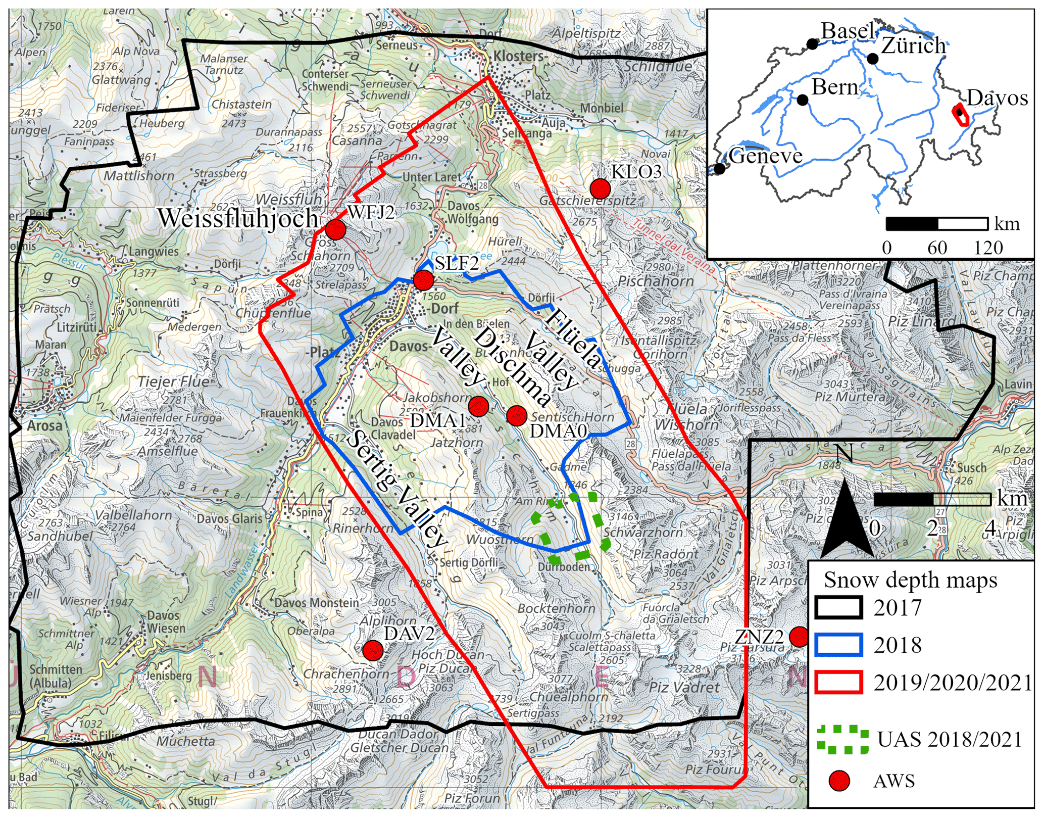
Figure 1 Overview of the study area. Snow depth map generated from the aeroplane imagery recorded in 2017 (black); extent of snow depth map from 2018 (blue); and snow depth area derived from the respective flights in 2019, 2020 and 2021 (red; corresponds to main study area). Additionally, the area covered by the UASs for reference data in 2018 and 2021 is shown (green). The red points symbolise the location of the AWSs with accurate snow depth measurements. The red polygon in the inset map depicts the location of the main study area in Switzerland (map source: Federal Office of Topography).

2 Study area Davos, Switzerland

The study area is located around Davos in Eastern Switzerland. A core area with an extent of approximately 230 km² was covered by all flight campaigns from 2019 to 2021. However, the total area acquired per year differs due to varying flight routes on each campaign (Fig. 1). The elevation of the main study area ranges from 1100 m a.s.l. around Klosters to the 3229 m a.s.l. high Piz Vadret. The diversity of the terrain, including extremely steep faces, large heterogeneous as well as open areas, settlements, forested areas, and glaciated areas can be considered representative for many mountainous regions. The research area is located in a transition zone between the humid north-Alpine climate and the drier climate zone of the central Alps (Kulakowski et al., 2011; Mietkiewicz et al., 2017). The main snowfall during the typical winter season is recorded at north-westerly and northern weather situations, which are commonly connected to strong storms with high wind speeds (Gerber et al., 2019; Mott et al., 2010).

3 Data and sensor

3.1 Vexcel UltraCam

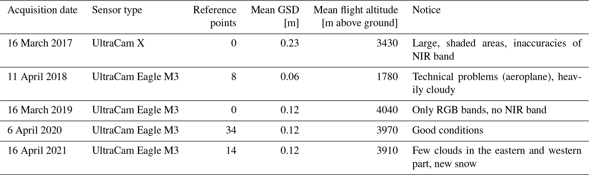
Airborne imagery was acquired with the large-frame camera series Vexcel UltraCam. The Vexcel UltraCam X was applied in 2017 and is characterised by a sensor pixel size of 7.2 µm × 7.2 µm, a focal length of 100.5 mm and a resolution of 14 430×9420 pixels (Schneider and Gruber, 2008). The UltraCam X was replaced by its successor, the UltraCam Eagle M3, in the following years. The UltraCam Eagle M3 is a state-of-the-art camera for photogrammetric measurements with 450 megapixels (MP) (Bühler et al., 2021). The improvements include a sensor pixel size of 4 µm × 4 µm, a focal length of 120.7 mm and a resolution of 26 000×14 000 pixels (Eberhard et al., 2021). Both UltraCam cameras acquire the four spectral bands red–green–blue (RGB) and near infrared (NIR) with a radiometric resolution of 14 bits. The camera positions are registered by differential Global Navigation Satellite System (dGNSS) mounted on the camera with a nominal accuracy of 0.2 m. The orientation of the camera is recorded through an inertial measurement unit (IMU) with a nominal accuracy of 0.01^∘ (omega, phi, kappa). These data simplify the determination of interior and exterior orientation and prevent tilts of the DSM.

The flights were conducted during the expected peak of winter (at approximately 2000 m) between March and April around midday to avoid large, shaded areas. The exact extent of each flight varied from year to year depending on the flight route and weather conditions (Fig. 1). The captured region in 2017 covered 600 km² (Fig. 1, black polygon) and was considerably larger than in the following years. High costs and limited flight permissions resulted in the selection of a smaller main study area (250 km² , red polygon) around Davos for the subsequent years.

Before the flights, reference points were marked with specially patterned tarps and measured by terrestrial dGNSS units with a vertical accuracy of 0.05 m. Because no reference points were acquired in 2017 and 2019, 10 extra reference points on conspicuous road markings were measured in retrospect. Different characteristics of each flight are described in Table 1.

Table 1 Properties of the executed annual UltraCam flights during the peak of winter.

3.2 Reference dataset

3.2.1 Airborne laser scanning (ALS) from summer 2020

Calculating snow depths with photogrammetric methods requires an accurate snow-off reference dataset. For the study area, an ALS point cloud from summer 2020 was available (Federal Office of Topography swisstopo, 2021a). The specified accuracies of at least 0.2 m in horizontal direction and 0.1 m in vertical direction comply with the requirements of accurate snow depth mapping. The point density of the ALS point cloud of at least 10 points m⁻² and on average 20 points m⁻² for all returns as well as 15 points m⁻² for ground returns allows a rasterisation of 0.5 m and the exact reconstruction of small-scale features as well as steep faces. The exact point classification enables the separation of vegetation, ground, buildings and water bodies. Correspondingly, a digital terrain model (DTM); a normalised ALS DSM, which only considered vegetation; and a normalised DSM, which only took buildings into account, were processed from the ALS point cloud. The ALS DTM also served as a reference dataset to evaluate the accuracy of the snow depth maps through the comparison of snow-free areas.

3.2.2 Unpiloted aerial systems (UASs) photogrammetry 2018 and 2021

To analyse spatial snow depths of small catchments, UAS-derived DSMs are commonly used, given the flexible acquisition at a vertical accuracy better than 0.1 m (Bühler et al., 2016). In order to compare snow depths derived from airborne data to UAS-derived ones, two UAS flights were carried out for a small subset (3.5 km²) in the Dischma valley during the UltraCam flight campaigns in 2018 and 2021 (Fig. 1, green polygon). In 2018 there was a small time lag (4 d) between UAS (eBee+ RTK) and airborne data acquisition. No significant snowfall but slightly positive temperatures (0 ^∘C level at 2500 m) were registered in between. In 2021, the UAS acquisition was conducted simultaneously with the UltraCam flight by the WingtraOne UAS with a 42 MP camera. The processing workflow of the UAS-derived DSMs was similar to the approach described in Eberhard et al. (2021), with the only difference being that outliers of the point cloud (less than three depth maps) were excluded.

3.2.3 Manual reference points

The manually measured reference points during the UltraCam flights had the purpose of serving as GCPs or check points (CPs). Due to the time-consuming fieldwork and avalanche danger, the number of reference points was limited, and they were often located close to roads in flat terrain. The 10 points measured in retrospect at distinctive locations were valid as reference, although they have a lower reliability compared to directly measured reference points. In 2020, during low avalanche danger, 34 reference points could be placed well distributed at different elevations and aspects.

Figure 2 Flowchart illustrating all processing steps for the creation of snow depth maps.

4 Methods

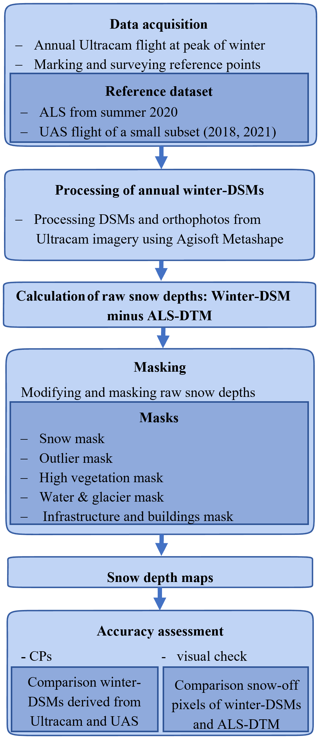
The creation of reliable and accurate snow depth maps consists of four steps (Fig. 2):

• processing airborne imagery and ALS point clouds,

• calculating snow depths,

• creating and applying necessary masks,

• checking the accuracy of the finalised snow depth maps.

The horizontal coordinate system CH1903+ LV95 and the height reference system LN02 were used to process the data. To ensure that the same coordinate system was used for all input data, conversions from other coordinate systems were carried out with the tool REFRAME (Federal Office of Topography swisstopo, 2021b) and transformations available in ArcGIS Pro 2.7. The airborne imagery was processed in Agisoft Metashape (version 1.6). It has proven its value in numerous snow-related studies (Avanzi et al., 2018; Bühler et al., 2016) and allows the processing of very large high-spatial-resolution airborne images (Eberhard et al., 2021; Meyer et al., 2022). The calculations and modifications of the snow depth values were carried out in ArcGis Pro.

4.1 Processing workflow of airborne imagery

Processing the aerial images in Agisoft Metashape is based on the structure-from-motion algorithm (Koenderink and van Doorn, 1991; Westoby et al., 2012). The general workflow is well explained in various publications (Adams et al., 2018) and the Agisoft manual (Agisoft LLC, 2020). However, applying the new sensor Vexcel UltraCam in combination with such a large and heterogeneous study area is sparsely explored. The workflow used in this study is based on Eberhard et al. (2021). However, the aim to use as few GCPs as possible to refine the orientation due to the limited availability of reference points required an adaption of this workflow.

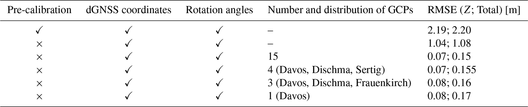
The Vexcel UltraCam camera is calibrated; hence, the interior orientation is known exactly. However, the application of the calibrated lens distortion parameters led to a large offset of the z value in the resulting DSM of approximately 2 m. Therefore, the interior and exterior orientation were calculated in Agisoft Metashape during the bundle-adjustment process (Triggs et al., 2000). Subsequently, the parameters for the interior and exterior orientations (especially focal length) were improved by the application of two to five GCPs. The necessary number of GCPs and the influence of their distribution for an exact and reliable orientation were determined by a parameter study for the UltraCam flight in 2020, which was characterised by 34 well-distributed reference points (Table A1). The quality grade was ascertained by the calculated RMSE of the CPs, which were not used for the orientation of the model (Agisoft LLC, 2020). This approach has shown that only one GCP is sufficient for a correct orientation and determination of atmospheric distortions under favourable acquisition conditions. Using more and well-distributed GCPs had no significant influence on the quality grade (Table 2). However, due to the high dependence on the precise measurement when using only one GCP and the possibility of varying atmospheric distortions when using cloud-covered images, we recommend the use of two to five GCPs. Warps and tilts, which often occur using a low number of GCPs with a limited dispersion over the area, were avoided on account of the exact coordinates of the shutter release points and camera rotation angles.

Table 2 Overview of the settings used and the corresponding accuracy (RMSE) for the parameter study for 2020.

The final DSMs with a point density from 5 points m⁻² (2017) over 20 points m⁻² (2019–2021) up to 90 points m⁻² (2018) and the corresponding orthophotos were exported with a spatial resolution ranging from 0.1 to 0.45 m depending on the average GSD. The workflow used is illustrated in Fig. 3, and further settings are described in Eberhard et al. (2021).

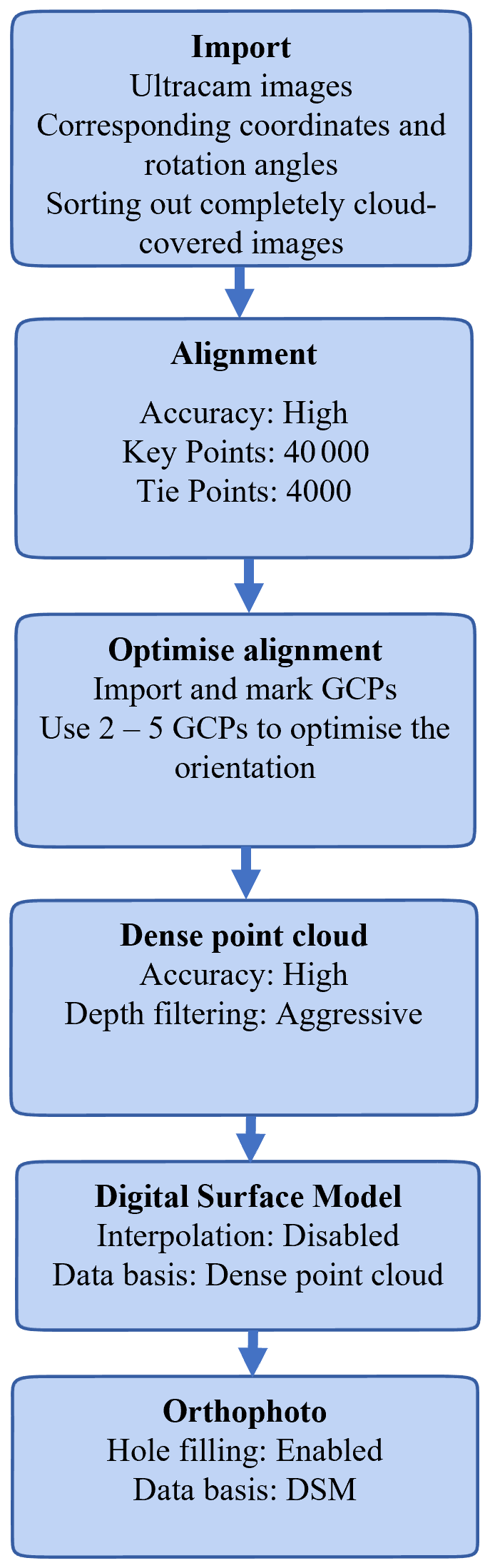
Figure 3 Flowchart illustrating the Agisoft Metashape parameter settings used to generate the winter DSMs from UltraCam imagery.

4.2 Creation of snow depth maps

The snow depths were calculated by subtracting the photogrammetric winter DSM from the ALS DTM, resulting in snow depth maps with a spatial resolution of 0.5 m, using the resampled winter DSMs. To avoid uncertainties based on misalignments between the winter DSM and the ALS DTM, we checked deviations of snow-free pixels in steep areas in each snow depth map. Since the deviations were small and the number of snow-free pixels in some years were limited, we did not perform a co-registration. The use of an ALS DTM was preferred because a DSM would underestimate the snow depths in open areas with low vegetation (Eberhard et al., 2021; Feistl et al., 2014). In addition, photogrammetric methods often struggle in dense and steep forests as well as in settlements in our study area, where the ALS DSM would have crucial advantages (Bühler et al., 2015). To get accurate and reliable snow depth maps, the application of various masks was required. Without the application of these masks, the average snow depth value of the study area would be overestimated by approximately 1 m, mainly caused by the forested areas.

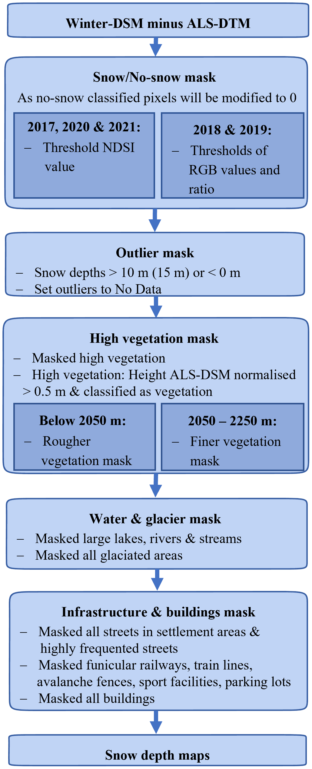
Figure 4 Flowchart illustrating the various masks used for the generation of reliable snow depth maps.

The procedure for developing these masks is based on the approach of Bühler et al. (2015), improved by Bührle (2021), and contains a snow mask, an outlier mask, a high-vegetation mask, a water-and-glacier mask, and an infrastructure-and-buildings mask. However, the existing algorithm to calculate the masks was adapted due to the use of the better UltraCam sensor and the availability of an accurate and well-classified ALS point cloud. An important goal for the procedure is the consistent and reproducible creation of the masks (Fig. 4). Additionally, excluding regions with heavy cloud cover led to more reliable snow depth values.

4.2.1 Snow mask

The snow mask has the aim to modify calculated snow depths of snow-free areas to zero (Bühler et al., 2016). Therefore, each pixel of the corresponding orthophoto is classified as snow-covered or snow-free, using the normalised difference snow index (NDSI) (Dozier, 1989; Hall et al., 1995) with a threshold around 0. This approach was applied for the years 2017, 2020 and 2021. An NDSI classification was not performed in 2019 due to technical issues that prevented the recording of the NIR band. In 2018, the NDSI method falsely classified pixels that exhibited snow mixed with soil as snow-free. Therefore, another classification method not relying on the NIR band and a better operation in snow mixed with soil was required. Since the blue band of snow exhibits higher reflectance than the red and green bands (Eker et al., 2019), a threshold of the ratio between the blue and red bands was used to determine the existence of snow. However, the values vary and depend on the strength of shadows; therefore, the thresholds were manually determined by an expert. To ensure the reliability of this approach, 500 random points in open terrain were selected and manually checked in the 2019 dataset, taking their correct classification into account.

4.2.2 Outlier mask

The outlier mask has the purpose to modify all unrealistic snow depth values, namely negative snow depths and extremely high snow depths above 10 m, to NoData. Only in the snow-rich year of 2019 was the upper limit adapted to 15 m, which had no significant impact on the outlier distribution.

4.2.3 High-vegetation mask

Due to uncertainties in the actual snow depth and problems with photogrammetric methods, areas with high vegetation were masked out. High vegetation, defined as vegetation with a height above 0.5 m, was identified through the vegetation classification and the calculated object height using the ALS point cloud. Additionally, a generalisation of the high-vegetation mask was required because wind, different sensor acquisition characteristics, and the varying time stamps of data acquisition between ALS and UltraCam affected the extent of high vegetation. The algorithm used for the generalisation differed between a rougher mask below 2050 m, where dense forests are predominant, and a finer mask above 2050 m, where free-standing trees and bushes are prevalent.

4.2.4 Water-and-glacier mask

The water-and-glacier mask prevents unrealistic snow depth values on water and glaciated areas. Due to low water levels during the peak of winter, the actual height of snow (HS) on frozen lakes is underestimated. Therefore, larger lakes, rivers and dominant streams were masked out. The data were obtained from the Swisstopo TLM3D geodata (Federal Office of Topography swisstopo, 2021c). Another problem is the significant volume loss of glaciers (approximately 2 m per year) in recent years (GLAMOS – Glacier Monitoring Switzerland, 2021). Accordingly, the calculated snow depths from 2017 to 2020 on glaciers are overestimated and therefore also masked out (Linsbauer et al., 2021).

4.2.5 Infrastructure-and-buildings mask

The infrastructure-and-buildings mask prevents distorted snow depths caused by buildings and temporary or moveable objects. Consequently, all buildings were completely masked out and infrastructure was partially masked. The buildings were derived from the classified ALS point cloud. The locations of technical constructions and infrastructure such as streets were obtained by the Swisstopo database. Railways, funicular railways, sport facilities, parking lots, all streets in settlement areas and main roads outside the settlements were masked out. Technical constructions like avalanche fences were also set to NoData. A very rough generalisation was used within dense settlements such as Davos, Arosa, and Klosters, whereas a finer generalisation was applied to areas beyond these settlements.

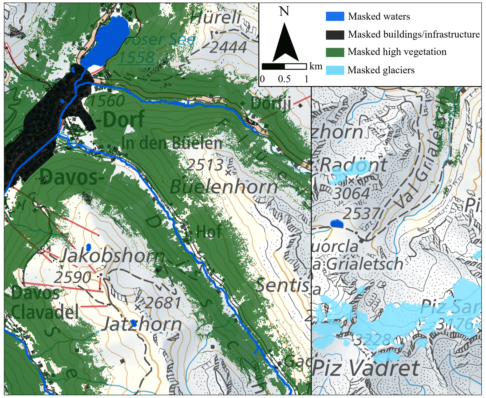
Figure 5 Spatial distribution of the masks used in selected extents of the main study area. Dark blue (water), light blue (glaciers), green (high vegetation) and black (buildings and infrastructure) polygons symbolise the different masks. Rivers are overrepresented for a better identification (map source: Federal Office of Topography).

4.2.6 Masking overview

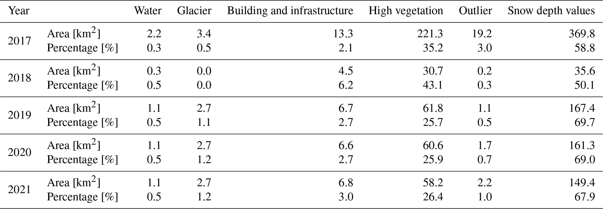
Using all presented masks (Fig. 5) on the raw snow depth values resulted in the final snow depth maps. The total area of the masks depends on the corresponding processing extent. For example, for the snow depth map from 2020, around 67 % of all pixels remained in the snow depth maps. A total of 28 % of the main study area was masked out as it belonged to high-vegetation areas. Only less than 1 % of the pixels were masked out as an outlier (Tables 3 and B1).

Table 3 Area [km²] and percentage [%] of various masks, outliers and remaining snow depth values for the 2020 snow depth map.

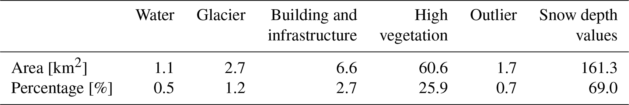
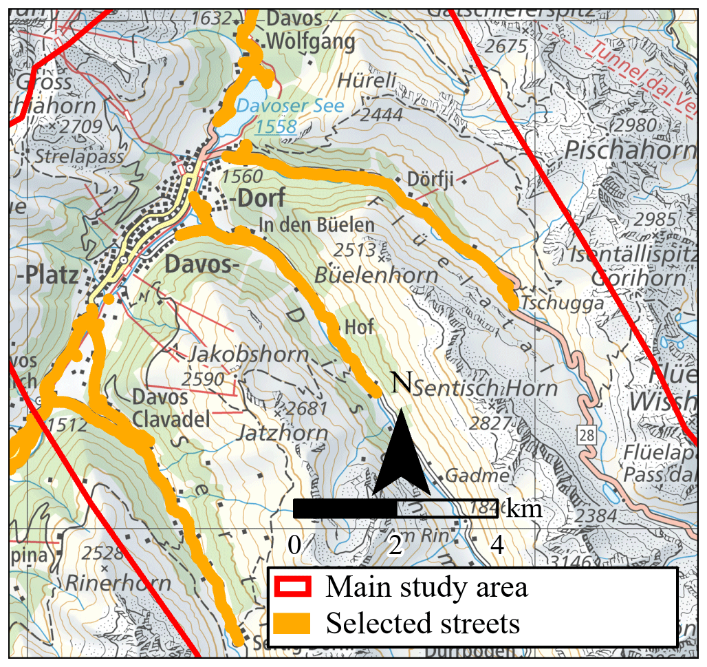
Figure 6 Overview roads used (orange lines) for accuracy assessment method 4; lines are overrepresented for better identification (map source: Federal Office of Topography).

4.3 Accuracy assessment

An essential part of this study is an extensive accuracy assessment of the snow depth values. Due to the absence of spatially continuous ground truth datasets, we determined the accuracy compared to several available reference datasets. The accuracy assessment consists of five different methods, which enabled a conclusive and spatially continuous evaluation of the annual winter DSMs. The selected quality procedures differ between the years and depend on the availability of reliable reference data (Table 4).

• The first method (M1) uses independent check points as validation (Sanz-Ablanedo et al., 2018). Even though the number of check points was limited and they were not well distributed over the entire study area, they are an important indicator for the correct orientation of the winter DSMs.

• In the second method (M2), due to their outstanding accuracy, UAS-derived DSMs serve as ground reference and enable direct and spatial comparison with UltraCam data over a small area (Deschamps-Berger et al., 2020; Marti et al., 2016).

• In the third method (M3), visual checks by an expert examined the plausibility of calculated snow depths and the correct application of the masks over the entire study area.

• Comparisons of snow-free areas on the winter DSMs with the reference ALS exhibited further evaluations. Method 4 (M4) determined deviations on the main roads beyond settlements which were always snow-free (Fig. 6). Extreme outliers exceeding 3 m (approximately MBE ±4 SD) were excluded, because bridges, tunnels and moveable objects led to higher deviations. M4 was applied in most of the snow depth maps, except 2019. In 2019, the absence of the NIR band in combination with puddles on the streets resulted in high deviations, which do not correspond to the actual accuracy. For a significant assessment, streets without puddles were manually digitalised and used as M4 in 2019.

• Method 5 (M5) considered deviations of all other snow-free pixels (M5) beyond settlements compared to the ALS DTM. Pixels with vegetation heights exceeding 0.05 m were excluded. Moreover, occasional and temporal changes of objects and infrastructure occurred between the acquisitions of the winter DSMs and the ALS DTM. Therefore, extreme outliers exceeding 3 m (approximately MBE ±4 SD) were excluded. Limited snow-free areas beyond streets in the winters of 2018 and 2019 impeded a meaningful evaluation of snow-free pixels in these years.

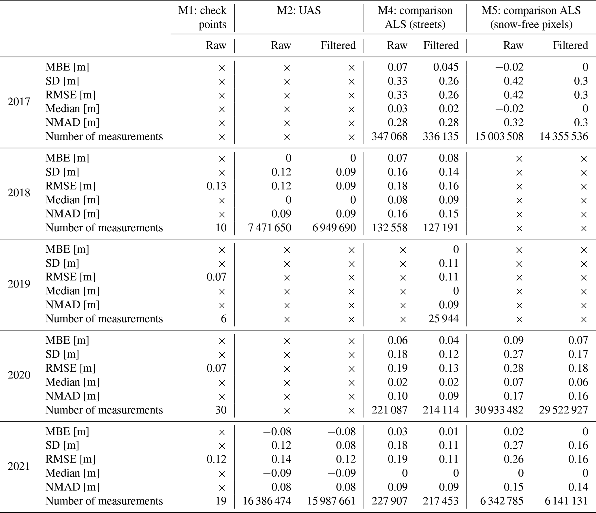
The quantitative procedures were evaluated by various commonly used statistical quality grades such as mean bias error (MBE), standard deviation (SD), RMSE, median and normalised median absolute deviation (NMAD) (details in Eberhard et al., 2021; Höhle and Höhle, 2009). The substantial impact of a few pixels with high deviations caused by the distortions described above led to the calculation of quality grades, excluding deviations beyond the confidence interval (MBE ±2 SD). Finally, since the accuracy of the snow depth values also depends on the reference ALS DTM, we examined the specified accuracy (Z=0.1 m) comparing 24 reference points (see Sect. 3.2.3) on snow-free areas with the ALS DTM.

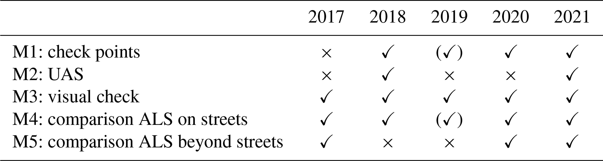
Table 4 Overview of the accuracy assessment methods performed in the different years.

5 Results and validation

5.1 Accuracy assessment

The quantitative part (M1, M2, M4, M5) of the accuracy assessment compares the deviations of the winter DSM to a selected reference dataset. As the horizontal accuracy of the check points (M1) of the winter DSMs was approximately 0.1 m in each year, which is also influenced by inaccuracies of the dGNSS, we especially focused on the vertical accuracy. The RMSE value comparing the ALS DTM to 24 reference points of 0.03 m demonstrates the high reliability of the reference ALS. The achieved accuracy of the reference DSMs derived from UASs was identified by using check points with an RMSE of 0.06 m (2021) and 0.1 m (2018).

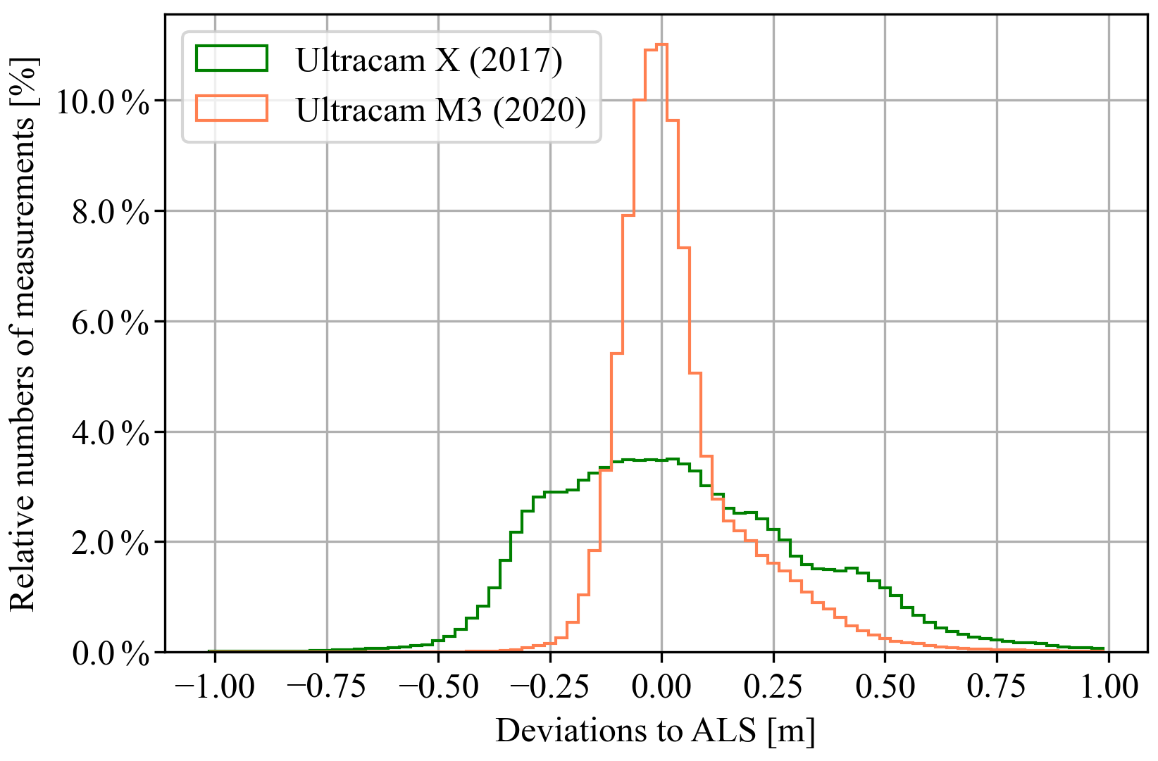
Figure 7 Comparison of the dispersion of deviations on streets to ALS between UltraCam X (green, 2017) and UltraCam Eagle M3 (light red, 2020).

5.1.1 2017

The accuracy assessment of the winter DSM 2017 calculates RMSE values of 0.26 m on open streets and 0.3 m on snow-free pixels after outlier removal (MBE ±2 SD) (Table 5). Resulting dispersions of M4 (SD = 0.33 m, NMAD = 0.28) and M5 (SD = 0.42 m, NMAD = 0.32) have considerably higher values compared to other years (see Sect. 3.1; Table 1). The same result can be clearly seen at the notably larger interquartile range of the winter DSM in 2017 in Fig. 10. Additionally, Fig. 7 shows the differences of the accuracy and the corresponding dispersion between UltraCam X and the successor UltraCam Eagle M3. The impact of the higher deviations is evident regarding the high number of outliers (3 %; negative snow depths) in steep and heterogenous terrain. Furthermore, inaccuracies of the NIR band led to insufficient classification of the snow mask. Accordingly, numerous pixels on streets, in transition zones of snow-free to snow-covered and in shaded areas are falsely classified as no snow.

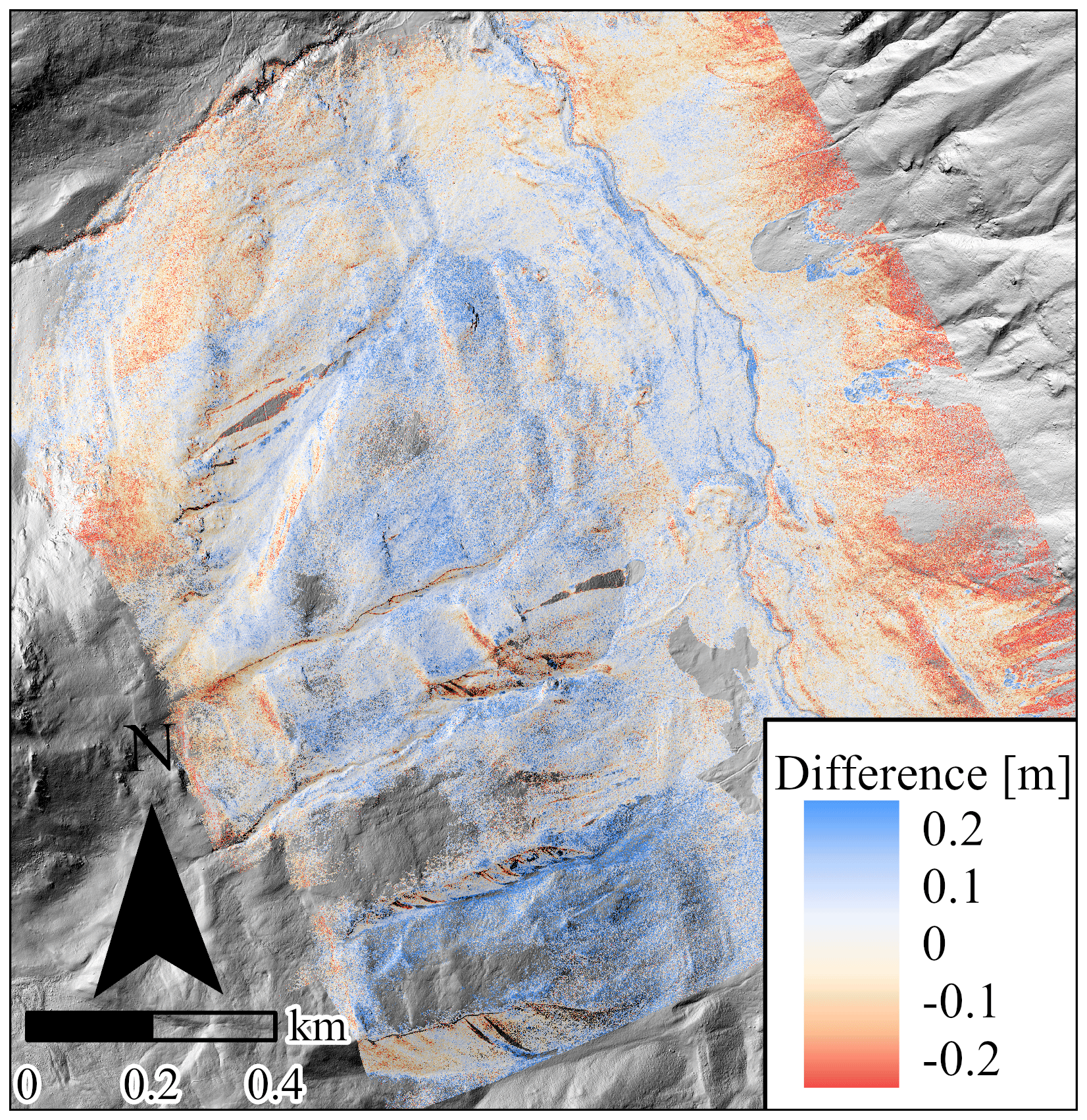
Figure 8 Difference calculation of the DSMs around the Schürlialp derived from UltraCam data and UAS in 2018.

5.1.2 2018

In 2018, large cloud-covered areas were excluded from the processing. Therefore, missing images and partly cloud-covered images resulted in reduced overlap in these regions. Nevertheless, the deviations of the 10 check points (RMSE 0.13 m) and the comparison with the UAS-derived DSM (raw = 0.12, filtered = 0.09 m) demonstrate a very high accuracy of the winter DSM (Table 5). The low aspect dependency of the deviations between UAS and UltraCam (Fig. 8) can be explained by the delay in capture time and therefore compression of the snowpack on south-facing slopes due to mild temperatures and strong solar radiation. The median of M4 (raw = 0.08, filtered = 0.09) shows a slight overestimation of the snow depths, which especially occurred south of Davos, close to cloud-covered areas. Despite these overestimations, the RMSE (raw = 0.18, filtered = 0.16) of the deviations on roads also proves the very high spatial reliability of the winter DSM. The classification of snow-covered pixels worked reliably; only isolated pixels in wet-snow avalanches, exhibiting a snow–soil mixture, were falsely classified.

5.1.3 2019

The occurrence of technical errors on the aeroplane prevented the capture of the NIR band, which can decrease the successful reconstruction of low-contrast snow surfaces and accordingly the accuracy of the DSM. However, no significant influence on the reconstruction or accuracy of the DSM was found. This high accuracy is confirmed by evaluations of the RMSE of the check points (0.07 m) and especially the RMSE of the manually digitalised snow-free areas (filtered = 0.11 m) (Table 5; Fig. 10). Using the snow mask also led to a high-quality grade of more than 99 % correctly classified pixels (method described in Sect. 4.2.1).

5.1.4 2020

The capture of the aerial images in 2020 was characterised by perfect acquisition conditions. Consequently, the winter DSM in 2020 evinces a very high accuracy of around 0.1 to 0.15 m, determined using 30 well-distributed CPs, which show an RMSE of 0.07 m (Table 5). The RMSE values of M4 also indicate a high accuracy (raw = 0.19, filtered = 0.13). Furthermore, the large snow-free areas in 2020 enable a representative accuracy assessment of M5, which considers deviations in different elevations and slopes. The RMSE of filtered deviations (0.18 m) in combination with the NMAD (0.16 m) of M5 shows the high reliability of the winter DSM in the entire study area and in steep terrain. The deviations of M5 in extremely steep areas (>40^∘) (filtered RMSE = 0.3 m) confirmed that the quality of the winter DSM decreases with increasing steepness but is still high (Bühler et al., 2015; Meyer et al., 2022).

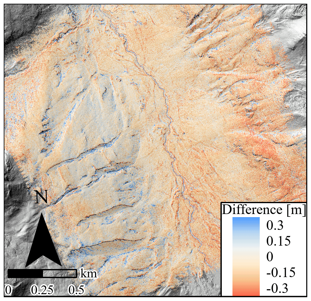
Figure 9 Difference calculation of the DSMs around the Schürlialp derived from UltraCam data and UAS in 2021.

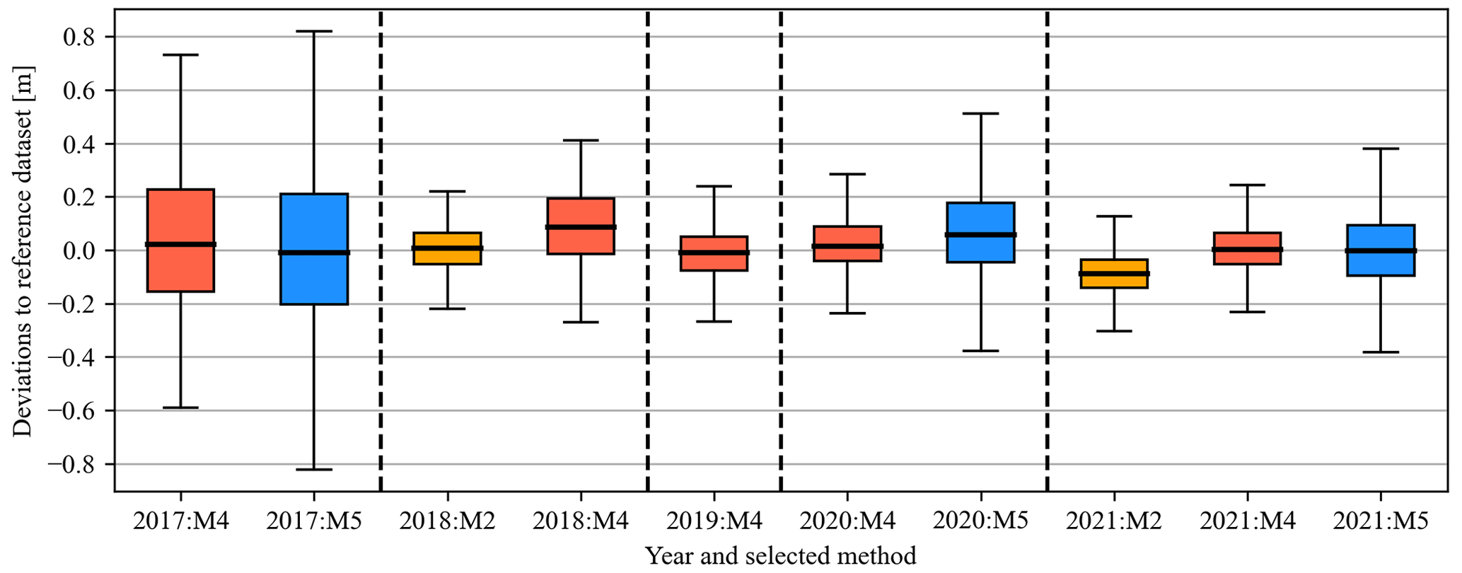
Figure 10 Box plots of the filtered deviations (MBE ±2 SD). Used methods: M2 (orange), M4 (red) and M5 (blue) for each year.

5.1.5 2021

In 2021, the surface above 1800 m a.s.l. was covered by a new snow layer, which caused less contrast during the UltraCam recording. Despite these difficult conditions, the analyses of the CPs indicate a high accuracy similar to that in 2020 (RMSE = 0.12 m). The RMSE (raw = 0.14, filtered = 0.12) values of the comparison between the DSMs derived from UltraCam and UAS also show very good results, with a slight tendency to underestimate the winter DSM (Fig. 9). The underestimation is characterised by a negative median (filtered $=-\mathrm{0.09}$). The median values of M4 (raw and filtered = 0) and M5 (raw and filtered = 0), however, show that this underestimation is a local problem and not valid for the entire study area. The RMSE values calculated with M4 (filtered = 0.11 m) and M5 (filtered = 0.16 m) demonstrate the very high accuracy of the snow depths (Table 5). Additionally, partly cloud-covered areas led to no significant increase in the dispersion, which is shown in the low NMAD values of M4 (raw = 0.09) and M5 (raw = 0.15).

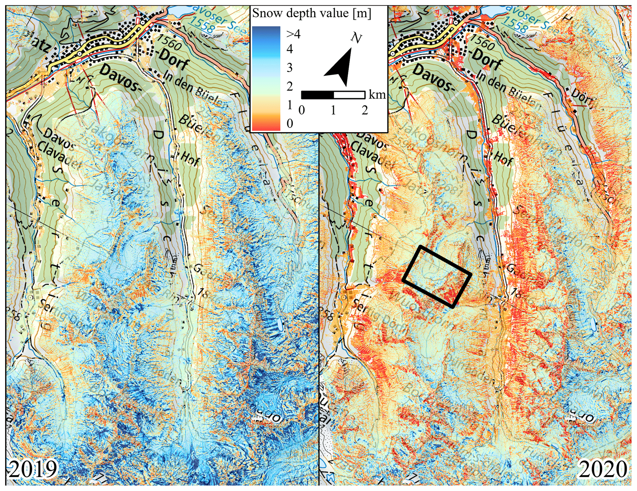
Figure 11 Comparison of an extent of snow depth maps from 2019 and 2020 during the corresponding peak of winter. The black polygon shows the location of the selected small catchment for a more detailed comparison between the available snow depth maps (Figs. 12, 13) (map source: Federal Office of Topography).

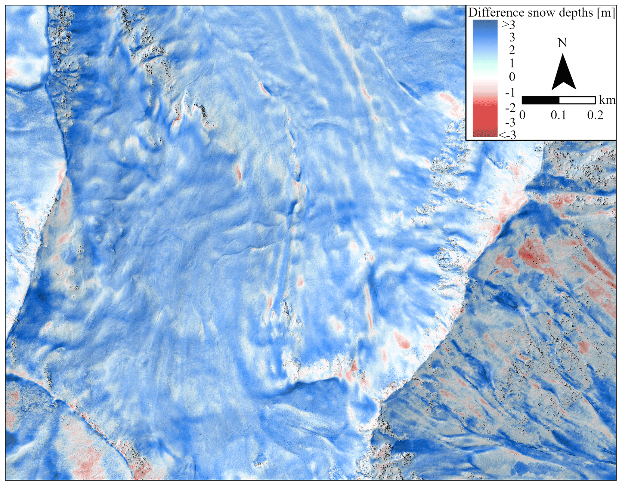
Figure 12 Difference calculation of the snow depth maps for 2019 and 2020 during the peak of winter in a small catchment (3 km²) close to Börterhorn. Black pixels symbolise NoData values.

Table 5 Overview and comparisons of the quality grades of the winter DSMs; column “Filtered” excludes outliers (MBE ±2 SD).

5.2 Snow depth maps

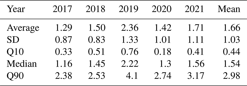
Despite varying and partly difficult acquisition conditions (Sect. 3.1) as well as some extremely steep and complex areas, on average, more than 99 % of the snow depth values in not-masked areas were successfully reconstructed. The image matching failed in a few overexposed or shaded regions only in the winter DSM from 2017. The high rate of success enabled the spatially continuous snow depth mapping of open areas around Davos. The spatial resolution of the maps (0.5 m) and the orthophotos (0.25 m) provide an excellent overview of the snow depth distribution within the study area. The existing level of detail shows numerous small-scale features over a large area and demonstrates the high variability of snow depths over small distances. Special characteristics of the study area are the strongly varying average snow depths and snow cover. The average snow depth values of the selected years ranged from 1.29 m in 2017 to 2.36 m in 2019 (Table 6). Comparing the 2019 and 2020 snow depth maps, significant differences in snow depth distribution and related features can be seen (Fig. 11). In 2019 the study area was almost completely snow-covered and exhibited numerous regions with high snow depths exceeding 3 m and was characterised by the occurrence of many slab avalanches. In contrast, the average snow depth in 2020 was considerably lower (1.42 m). The study area was often characterised by snow-free slopes below 2400 m a.s.l. in southern aspects as well as numerous glide-snow and wet-snow avalanches.

Furthermore, the aspect dependence of the snow depths was more pronounced in 2020 than in 2019.

Despite the high difference of the average snow depth values between these 2 years, similar patterns in the relative snow depth distribution and occurrence of special features are identifiable. In general, the snow depths in both years increase with rising elevation until a certain level close to ridges or peaks. Higher snow depths are more frequently found on northern aspects compared to south-facing slopes, which shows the aspect dependence of snow depths. Furthermore, higher and lower relative snow depths of both snow depth maps occurred at similar locations (Fig. 11).

Table 6 Overview average snow depths [m], standard deviation [m] and different quantiles (10 %, 50 %, 90 %) [m] of each annual snow depth map.

To confirm these observations on a smaller scale, we further looked into the detailed differences of these snow depth maps by calculating the differences of the HS for a small high-mountain catchment (3 km², Fig. 12). Generally, the snow depth values in 2019 were mostly higher than in the following year. However, annual differences can strongly vary within short distances, and in a few locations the snow depth in 2020 was as high as or higher than in 2019. These pixels were especially located in exposed areas close to the ridge or in release zones of glide-snow avalanches. Considerable differences between these 2 years were the extent of cornices and the consideration of snow depths in avalanche accumulation zones.

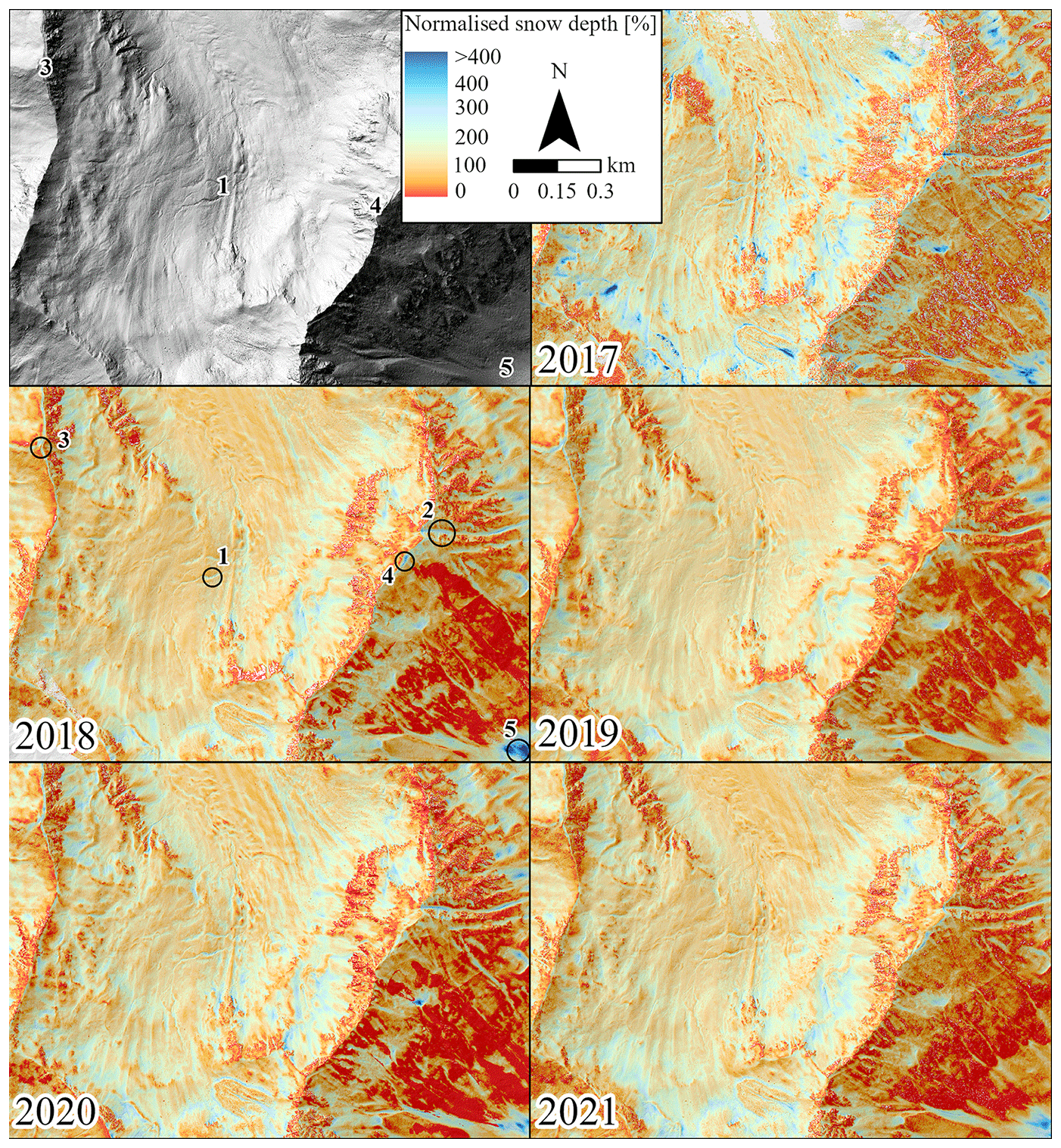
Figure 13 Comparison of the normalised snow depth maps of the 5-year period (2017–2021) during the peak of winter in a small catchment (3 km²) close to Börterhorn. Numbers in the hillshade highlight different special features, which demonstrate the existing grade of detail: (1) filled small creeks, (2) filled drainages in an extremely steep area close to Börterhorn, (3) remarkable cornice between Tällifurgga and Witihüreli, (4) cornice between Wuosthorn and Börterhorn, and (5) deposition zone of avalanches. White pixels in the snow depth maps symbolise NoData values.

To investigate the snow depth distribution patterns, we compared the relative snow depth distribution between the years. The normalised snow depth values of each year were calculated by the relation of the HS in contrast to the average snow depth of the selected area in the corresponding year. The normalised snow depth maps have the advantage of being independent from differences in the absolute snow depth between the years, which enables a better overview of the actual snow depth distribution. As exemplarily depicted in Fig. 13, we observed similar distribution patterns between all years. Generally, higher relative snow depths often occurred at deposition zones of avalanches, along terrain edges in wind-protected zones and within sinks. Lower snow depths were frequently observed on slopes exceeding 35^∘, in wind-exposed areas and in the release zones of avalanches (see also Sect. 6.2.3). However, a few features such as avalanches in certain tracks only occurred in some years.

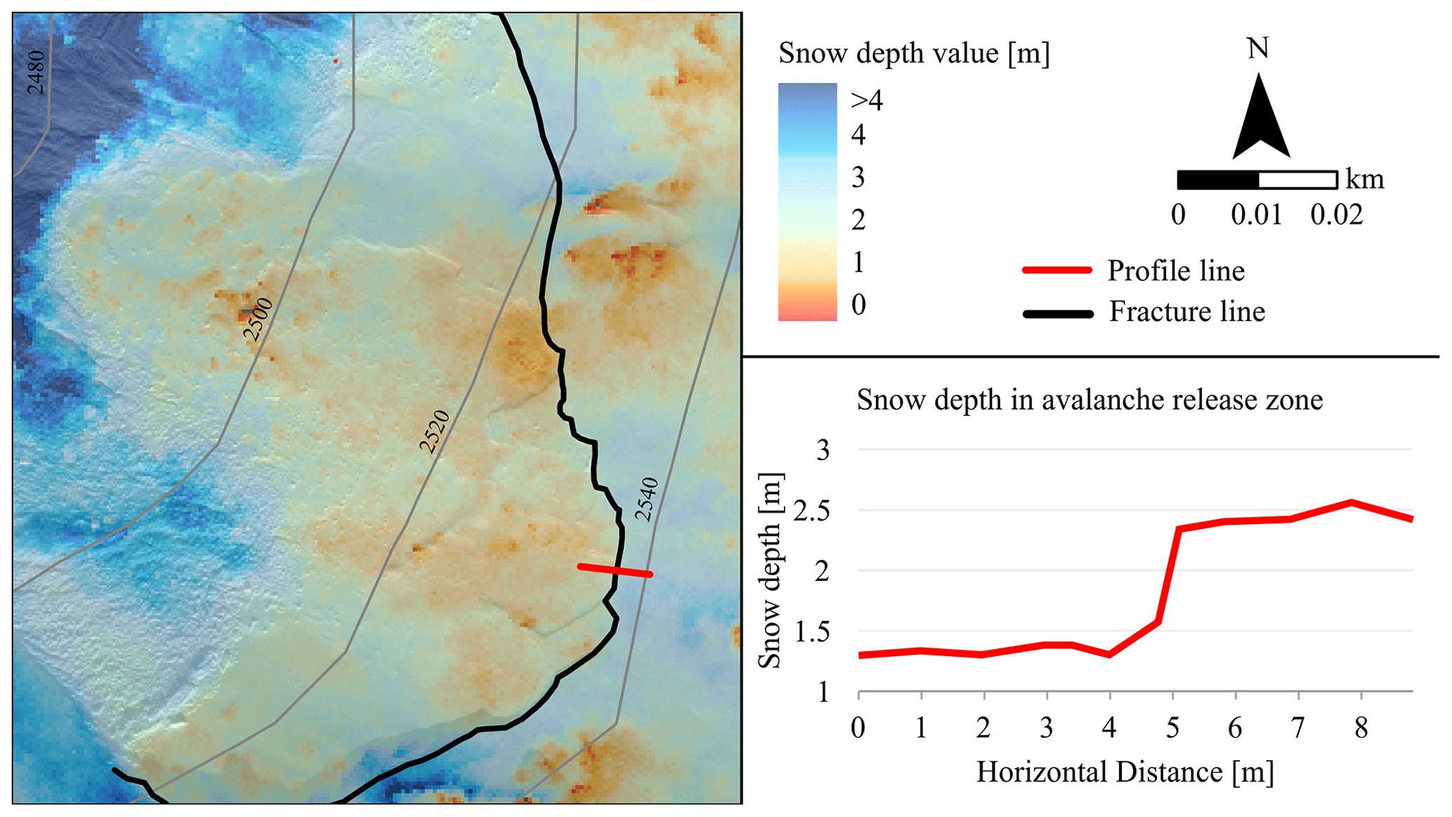
Figure 14 Overview of the snow depth distribution of the release zone of a slab avalanche close to Börterhorn (Dischma valley) captured by the UltraCam in 2019; the red line symbolises a height profile showing the course of snow depth values vertical to the fracture line; the prominent difference in snow depths indicates the release height of around 0.95 m.

The detailed detection of numerous avalanches by means of the snow depth maps and corresponding orthophotos is a salient characteristic of the data. In particular, glide-snow avalanches, striking slab avalanches and deposition zones of wet-snow avalanches can be identified. The investigation of the snow depth distribution around the fracture line enables the calculation of the release height. As shown in Fig. 14, the release height of this slab avalanche was approximately 0.95 m.

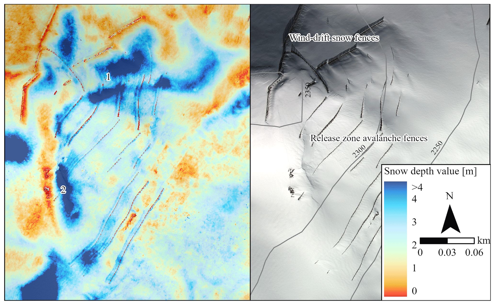
Figure 15 Snow depth distribution and corresponding orthophoto around avalanches fences at Grünihorn, captured by the UltraCam flight on 16 March 2019. The numbers 1 and 2 indicate buried avalanche fences with snow depths exceeding 5 m.

To present additional applications of our snow depth maps, we exemplarily assessed snow depth distribution around different avalanche protection structures. Therefore, the workflow was slightly adapted by unmasking the avalanche fences. In 2019, the UltraCam recording took place shortly after a large snowfall (1.3 m new snow at Weissfluhjoch within 7 d) during a snow-rich winter. The orthophoto and corresponding snow depth map show that large parts of the release-zone avalanche fences, south of the wind-drift snow fences (1), were completely buried as snow accumulated up to 6 m (Fig. 15). The avalanche fences close to the ridge (2) were also covered by a prominent cornice with a snow height of 5.5 m.

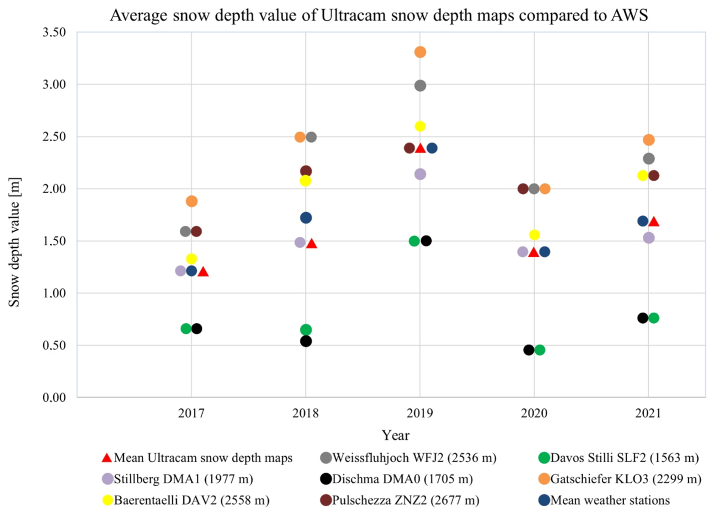
Figure 16 Average snow depth value from the UltraCam snow depth maps (red triangle, core area) compared to snow depth measurements from automatic weather stations (circles) during the UltraCam flights. Locations of the AWSs are shown in Fig. 1. Blue circles symbolise the mean of all AWS snow depth measurements.

We also compared the average snow depth value of the different snow depth maps (core area) with the punctual snow depth measurements from the eight AWSs around Davos, which are well distributed at different elevations and aspects in our study area (Fig. 1). Despite the large differences in snow depths between the years, the average value of all AWSs was similar to the average value (±0.07 m on average) derived from our snow depth maps (Fig. 16). Only in 2018, when the main part of the higher mountains was cloud-covered, was our value considerably lower (−0.22 m) compared to the mean snow depth measurements from the AWSs.

AWS snow depth measurements are supposed to yield typical snow depth. Hence, finding a suitable location for a new AWS is a matter of finding an ideal location with representative snow height in the area of interest. To facilitate this decision-making process, SLF developed a model, considering snow depth, to assess the suitability for a new station in the Dischma valley. Regarding the snow depth distribution, the model assesses the representativity of the measured snow depth for the area (Fig. 17). In addition, the model also considers different topography parameters such as roughness, avalanche danger (Bühler et al., 2022) and slope gradient.

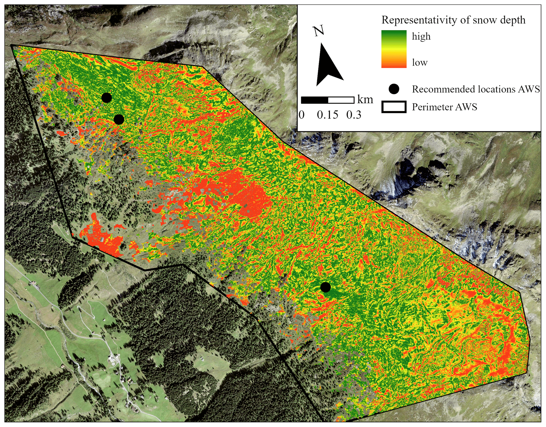
Figure 17 Representativity of punctual snow depth measurements (possible locations for AWSs) for the entire perimeter (black polygon) derived from aeroplane snow depth maps. Black circles symbolise predefined locations for the AWSs. The south location was finally selected due to its high representativity (dark green), low avalanche danger and flat terrain for the new AWS Luksch Alp (map source: Federal Office of Topography).

6 Discussion

In this study we present results from annual UltraCam campaigns (2017 to 2021) to generate high-resolution snow depth maps. We investigated the necessary processing steps to derive accurate winter DSMs, to apply required masks and to assess the characteristics of the resulting snow depth maps. We analysed the accuracy and validity of the resulting winter DSMs and used the snow depth maps for different applications. In this section, we discuss the obtained results.

6.1 Processing of snow depth maps

This study focussed on the accurate and consistent processing of large-scale snow depth maps under different acquisition conditions with the new Vexcel UltraCam sensors over a period of 5 years. We have observed a significant quality increase from the Vexcel UltraCam X to the successor Eagle M3 due to its higher GSD and better radiometric characteristics. Data from the UltraCam X in 2017 exhibited errors in the NIR band, which complicated the classification of snow-free pixels. The RGB sensor of the UltraCam X was partly overexposed; hence, Agisoft Metashape had problems finding matching points in a few sunlit snow areas. The accuracy assessment in 2017 shows that the RMSE (∼0.25 m) of the winter DSM is significantly poorer than in the following years (Table 5; Fig. 10), which is no noticeable advance compared to other studies (Bühler et al., 2015; Nolan et al., 2015).

With the new Vexcel UltraCam Eagle M3 sensor, Agisoft Metashape was able to reconstruct almost the complete surface, even in heavily shaded areas, on surfaces covered by fresh snow as well as in partly cloud-covered regions. A similar successful processing of small catchments was achieved by Meyer and Skiles (2019). However, our approach still reveals a significant progress in photogrammetric snow depth mapping compared to other large-scale snow depth maps from previous studies (Bühler et al., 2015; Nolan et al., 2015). Using the UltraCam Eagle M3 also resulted in a considerably better GSD at similar flight altitudes compared to recent studies (Meyer et al., 2022). The better GSD enables the exact processing of snow depth maps with a spatial resolution of 0.5 m, which can be considered an improvement regarding large-scale snow depth maps and capturing the small-scale distribution pattern accurately (Miller et al., 2022). The extensive accuracy assessments have shown a high reliability of the processed winter DSM based on the Vexcel UltraCam Eagle M3 sensor with an accuracy of approximately 0.15 m (Fig. 10). The accuracy assessment of the reference ALS DTM compared to reference points (RMSE 0.03 m) has also demonstrated its high reliability. Therefore, the accuracy achieved in the winter DSMs corresponds approximately to the actual accuracy of the calculated snow depth values. These accuracies of the snow depths match with the best results in Eberhard et al. (2021) and Meyer et al. (2022).

The strength of the presented workflow is its robustness, demonstrated by the quality grades of the snow depth maps despite difficult and complex acquisition conditions in high-mountain regions. In addition, excellent acquisition conditions such as in the year 2020 resulted in no significant improvements to the quality metrics.

A crucial disadvantage of our workflow compared to the one of Meyer et al. (2022) is the necessity of two to five GCPs. Little effort was needed to measure the GCPs in the present study area due to their vicinity to the settlement, but this might be a limitation elsewhere. This could be solved by using a global coordinate system, but first experiences have shown that the accuracy is lower and less reliable compared to our workflow. Under consideration of this limitation, the procedure is applicable to different study areas.

Compared to more expensive, ALS-derived snow depth maps (Bühler et al., 2015; Deems et al., 2013; Painter et al., 2016) our computed metrics demonstrate an equal accuracy. However, in areas with high vegetation or dense forests, it is currently not possible to derive snow depths through photogrammetry. Different approaches have been proposed to obtain snow depth with photogrammetric methods within forested areas (i.e. Broxton and van Leeuwen, 2020; Harder et al., 2020), yet the steep slopes in combination with dense forests around Davos impeded the processing.

To counteract false values in those problematic areas, a similar masking approach to ours was previously applied in Bühler et al. (2015), but the algorithm we used has been considerably improved and is more reliable. The masks that we processed consistently and reproducibly are characterised by a high accuracy but also exhibit few errors and limitations. In total, the percentage of incorrectly masked areas amounts to less than 1 %, which is considered satisfactory. The errors include, for example, snow-covered pixels in heavily shaded areas and snow mixed with soil falsely classified as no snow. Additional errors were caused by new buildings, ignored single trees or environmental changes resulting from mass movements. As those changes are inevitable in our study and the values only account for a small proportion of our masks, we assess their effects as negligible. The transferability of the masks to other study areas depends on the data availability of existing forests and settlements.

6.2 Applications

The remarkable characteristics of the snow depth maps and the corresponding orthophotos enable new possibilities for various applications in science and practice: the assessment and prevention of natural hazards, research on snow depth distribution processes, and snow hydrological models as well as other measurement methods. In the following sections we would like to discuss the relevance and potential impact of our work on selected applications.

6.2.1 Natural hazards

The investigation of natural hazards such as snow avalanches or snow loadings on buildings can benefit from the presented snow depth maps and the approach applied. Studies of Bühler et al. (2019), Hafner et al. (2021), Eckerstorfer et al. (2019) and Leinss et al. (2020) have already demonstrated the importance and limitations of manual as well as automatic large-scale avalanche mapping with satellite data. On a smaller scale Korzeniowska et al. (2017) proved the automatic detection of avalanches on the basis of orthophotos derived from airborne photogrammetry (sensor ADS80). Due to better radiometric characterisations and better spatial resolution of our orthophotos, more details could be obtained than in previous studies. Furthermore, different studies (i.e. Peitzsch et al., 2015) have already suggested that the locations of glide-snow avalanches are often similar between winters. Our data series confirms this finding.

As shown in Fig. 14, the high-resolution orthophoto allows for the exact identification of snow avalanches and associated release and deposition zones over larger regions. In numerous cases, the detection of the fracture line of an avalanche is possible as well. Consequently, the snow depth distribution around the avalanche fracture line can provide meaningful information about the release height and volume. However, release zones covered by new or wind-drifted snow or avalanches released in extremely steep and complex terrain can be difficult to identify. Nevertheless, these snow depth maps are the first study to enable the determination of release heights of distinctive avalanches over larger regions. Since so far only individual studies with UASs were able to accurately identify the release height (Souckova and Juras, 2020; Proksch et al., 2018; Bühler et al., 2017), this is a considerable improvement. Furthermore, the assessment of snow volumes in release and deposition zones based on snow depth maps and orthophotos facilitates research on avalanche activity and characteristics of the corresponding period. Studies with UASs have already demonstrated the high importance of these measurements (Bühler et al., 2017; Eckerstorfer et al., 2016).

The crucial advantage of our procedure compared to previously performed studies with UASs is the ability to cover larger areas during periods with high avalanche activity. However, the necessity of the flight permission and the weather dependence often prevent short-term missions.

The assessment of other hazards such as snow loading on buildings or flooding caused by rapid snow melt can also be assisted by large-scale snow depth maps. For the determination of snow loads on buildings, an adaption of our workflow would be required by using the DSM as a reference dataset and refraining from masking out settlements.

6.2.2 Planning and evaluation of avalanche protection structures and automatic weather stations

Avalanche fences and other avalanche protection structures are crucial in Alpine regions for the protection of infrastructure and residents. However, the functionality of avalanche fences is only guaranteed if they are correctly placed and have a sufficient height (Margreth, 2007). In our case, the snow depth map in 2019 demonstrates that the investigated wind-drift snow fences are located too close to the release zone (Fig. 15). This increases the snow accumulation within these areas (Bühler et al., 2018a) and reduces the protective effect. Since large parts of the fences were buried by snow in 2019, the current fences may not be sufficient to prevent avalanche releases during critical periods. Accordingly, the snow depth maps can be used for large-scale evaluation of existing and planned avalanche protection structures (Prokop and Procter, 2016). Switzerland has acknowledged the importance of snow distribution for the planning, and therefore snow depth maps are established in the construction process.

Furthermore, the snow depth representativity map (Fig. 17) demonstrates how our snow depth maps can be used in models to evaluate existing AWS sites and facilitate the identification of potential locations for new AWSs, which play a key role for different forecasts such as the avalanche warning service (Pérez-Guillén et al., 2022). Our snow depth maps led to the assessment of a suitable location with a high representativity for the new AWS Luksch Alp (Dischma valley), which was built in 2022. Similar snow depth maps as well as the gained knowledge about snow depth distribution pattern will be applied for the planning of new AWSs.

In addition, our snow depth maps enable the assessment of existing long-term AWSs around Davos, which are used for various projects and avalanche forecasting. Previously, the representativity of these stations was assessed qualitatively by experts, but now our snow depth maps enable the comparison of spatial snow depth measurements in open areas with the station measurements (Fig. 16). However, the presented results only represent the peak-of-winter date; accordingly, during the early winter or melt season, the relation between point snow measurements to spatial snow depth distribution could be different due to changing energy balances. Further investigations are required to confirm similar snow depth distribution pattern over the entire winter season and to enable accurate interpolations from point measurement (AWS) to entire catchments.

6.2.3 Analysis of specific snow depth distribution features

Our snow depth maps play a key role in better understanding the snow depth distribution in Alpine terrain. The results presented in Fig. 11 and Table 6 show the strongly varying average snow depths and point out the added value of annual snow depth maps (Marty et al., 2019). Despite the high difference of the average snow depths, we identified a similar relative snow depth distribution (Fig. 13). Consequently, the relative snow depth distribution between different years is almost independent of the average snow depths except for separate avalanche depositions zones and selected special features as they do not occur every year.

The studies of Grünewald et al. (2014) and Prokop (2008) found that snow at wind-exposed and steep areas is relocated to flatter areas and sinks. Our results confirm these observations. For example, small creeks in high-mountain catchments can be identified in our snow depth maps because the creeks are filled with snow. Similar features can be recognised in drainage channels.

Bühler et al. (2015) and Schirmer et al. (2011) recognised the re-occurrence of cornices at the same ridges within our study area in 2 different years. Our data can verify the formation of this cornice in subsequent years. In addition, we determine the re-occurrence of cornices at the same locations in all of our assessed years. These cornices lead to considerably higher snow depths on the same side in each winter.

Our observations concerning the relative snow distribution correspond to the results of Schirmer et al. (2011) and Wirz et al. (2011), which found higher and lower relative snow depths on the same locations within a winter. However, all these studies were either temporally limited to only 1 year (Schirmer et al., 2011; Wirz et al., 2011) or the accuracy and the spatial resolution of the snow depth maps (Bühler et al., 2015; Marty et al., 2019) complicated the investigation of snow depth distribution patterns. Therefore, our snow depth maps are the first time series which enables an extensive large-scale comparison of snow depth distribution between different years. These new possibilities lead to the confirmation of different theoretical approaches, which assume that snow depth distribution is more dependent on terrain characteristics than on the weather conditions of a certain year. This finding opens new possibilities for modelling snow depths over large regions.

6.2.4 Validation and snowpack modelling approaches

Different studies have already benefited from the existing unique time series of large snow depth maps (pushbroom scanner ADS) presented by Marty et al. (2019). However, the inaccuracies and lower reliability of these snow depth maps also limited the validation and evaluation of other studies. Deep learning approaches (Daudt et al., 2023) or studies which are calibrated by exact reference data can now benefit from our improved quality. Therefore, it is to be expected that our data and approach will be used in numerous studies. For example, the snow depth maps serve as training dataset for a running project to improve the modelling of the daily snow depth distribution in Switzerland. Without our data, the model was not able to represent the snow depth distribution in complex terrain. In addition, our data could correct modelled snow depth maps which, for example, often exhibit a bias towards an overassessment of snow depths in high-mountain region.

Our data could also validate or evaluate numerous projects in conjunction with hydrological and snow modelling (Helbig et al., 2021), wind-drift models (Gerber et al., 2017; Mott et al., 2010; Schön et al., 2015), automatic detection of avalanche release zones (Bühler et al., 2018b; Bühler et al., 2022), and further snow depth models or snow depth measurements on the basis of satellite data (Leiterer et al., 2020; Wulf et al., 2020). Additionally, they can improve critical input parameters (Vögeli et al., 2016) to better represent different processes in various snow hydrological models.

7 Conclusions

In this study we present the development, validation, and application of a consistent and robust workflow to process aerial imagery from the state-of-the-art large-format camera Vexcel UltraCam to produce reliable snow depth maps. We demonstrate its capability to capture large areas covering more than 100 km² under optimal and suboptimal acquisition conditions (varying illumination, clouds, new snow cover, absence of the NIR band). The accuracies of our snow depth maps (RMSE: 0.15 m, UltraCam Eagle M3) are similar to results achieved with ALS and fulfil the requirements for meaningful, spatially continuous snow depth mapping in complex, open terrain. The metrics were calculated by applying an extensive accuracy assessment with CPs, comparisons to UAS-derived DSMs and the evaluations of snow-free pixels, revealing a very high quality even within steep terrain. The reliability of our maps allows for the comparison of snow depth values within a 5-year period, which have shown that despite large differences of the average snow depth, the relative snow depth distribution and the formation of small-scale features are similar throughout the years.

Restrictions of the data and its acquisition are the relatively high data acquisition costs (approximately CHF 20 000 for 300 km²) and the availability of a piloted aircraft and corresponding permissions. In addition, the procedure is limited by widespread low clouds, areas with high vegetation such as forests, the availability of accurate snow-free DTMs and powerful hardware. Even though accurate dGNSS and IMU data are available from the aeroplane, one to five ground control points (GCPs, distribution is not important) and the consistent calculated masks are essential to achieve reliable results.

In particular, the high spatial resolution of our maps (0.5 m) and orthophotos (0.25 m), in conjunction with the achieved accuracy, offers the possibility to better understand the complexity of snow depth distribution in high-mountain regions. Based on the presented products, models which use snow depths to assess the water stored in the snowpack (SWE) can be further evaluated and improved; however, the determination of the SWE still depends on assumptions for the snow density and exhibits various uncertainties. Nevertheless, the better assessment of SWE is, for example, crucial for hydropower generation. New approaches to map snow depth with optical and radar satellites from space can be evaluated. Also, the investigation of snow avalanches benefits from such data. Several running research projects are already applying our maps for validation. We expect that in the coming years our data will play a key role in numerous new findings in snow science.

The improvement of photogrammetry within Alpine forests would be a significant step forward to equalise with the advantages of ALS. Our data allow for the extrapolation of the snow depth distribution from small areas mapped, for example, by UASs to the scale of large catchments. To further enhance the value of photogrammetric snow depth mapping, the current time series will be extended into the future. Together with datasets acquired from 2010 to 2016 with the ADS within the same region, we established a unique 11-year snow depth time series.

Appendix A: Overview reference points in 2020

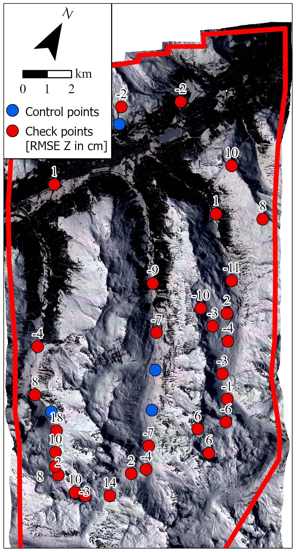
Figure A1 Overview of the distribution of ground control points (blue) and check points (red) with the corresponding RMSE Z values. Background shows the orthophoto from 2020.

Appendix B: Overview area and percentage of masks used for the corresponding snow depth maps

Table B1 Area [km²] and percentage [%] of various masks, outliers, and remaining snow depth values for all snow depth maps.