Modelling the development and decay of cryoconite holes in northwestern Greenland

Cryoconite holes (CHs) are water-filled cylindrical holes with cryoconite (dark-coloured sediment) deposited at their bottoms, forming on ablating ice surfaces of glaciers and ice sheets worldwide. Because the collapse of CHs may disperse cryoconite on the ice surface, thereby decreasing the ice surface albedo, accurate simulation of the temporal changes in CH depth is essential for understanding ice surface melt. We established a novel model that simulates the temporal changes in CH depth using heat budgets calculated independently at the ice surface and CH bottom based on hole-shaped geometry. We evaluated the model with in situ observations of the CH depths on the Qaanaaq ice cap in northwestern Greenland during the 2012, 2014, and 2017 melt seasons. The model reproduced the observed depth changes and timing of CH collapse well. Although earlier models have shown that CH depth tends to be deeper when downward shortwave radiation is intense, our sensitivity tests suggest that deeper CH tends to form when the diffuse component of downward shortwave radiation is dominant, whereas CHs tend to be shallower when the direct component is dominant. In addition, the total heat flux to the CH bottom is dominated by shortwave radiation transmitted through ice rather than that directly from the CH mouths when the CH is deeper than 0.01 m. Because the shortwave radiation transmitted through ice can reach the CH bottom regardless of CH diameter, CH depth is unlikely to be correlated with CH diameter. The relationship is consistent with previous observational studies. Furthermore, the simulations highlighted that the difference in albedo between ice surface and CH bottom was a key factor for reproducing the timing of CH collapse. It implies that lower ice surface albedo could induce CH collapse and thus cause further lowering of the albedo. Heat component analysis suggests that CH depth is governed by the balance between the intensity of the diffuse component of downward shortwave radiation and the turbulent heat transfer. Therefore, these meteorological conditions may be important factors contributing to the recent surface darkening of the Greenland ice sheet and other glaciers via the redistribution of CHs.

1 Introduction

Cryoconite holes (CHs), cylindrical water-filled holes formed on ablating ice surfaces of glaciers and ice sheets worldwide, influence the ablation process of glacial ice and function as the habitats of glacial microbes (e.g. Hodson et al., 2010a; Cook et al., 2016; Uetake et al., 2016; Zawierucha et al., 2021). In CHs, dark-coloured sediment, referred to as cryoconite, is deposited at the bottom; it consists mostly of spherical aggregates (cryoconite granules) formed by the entanglement of filamentous cyanobacteria with mineral and organic particles (Hodson et al., 2010b; Langford et al., 2010; Takeuchi et al., 2010, 2014; Wientjes et al., 2011; Uetake et al., 2019). Because such dark-coloured sediment on bare ice absorbs solar radiation more effectively than the surrounding clear ice, CH formation occurs often.

The development and decay of CHs depend on the meteorological conditions near the ice surface. CHs are likely to form well under sunny conditions (McIntyre, 1984; Fountain et al., 2008; Jepsen et al., 2010; Cook et al., 2016; Takeuchi et al., 2018). Although many studies have investigated which meteorological conditions are favourable for the deepening (development) of CHs, there is limited information on their shallowing (decay) dynamics. Takeuchi et al. (2018) reported that CHs collapse under cloudy and windy conditions in summer in northwestern Greenland. They suggested that CHs collapse when the ice surface surrounding the CHs experiences enhanced melt caused by turbulent heat flux exchange. CH collapse events have also been reported in Svalbard and southwestern Greenland (Hodson et al., 2007, 2008; Stibal et al., 2008; Irvine-Fynn et al., 2011; Chandler et al., 2015), while it has been indicated that a higher melt rate at the ice surface induces CH collapse (Hodson et al., 2007).

The development and decay of CHs modulate the ice surface albedo. On the one hand, the development of CHs increases the area-averaged ice surface albedo compared to the case where the surface is uniformly covered with cryoconite granules because cryoconite granules in holes are shielded from sunlight by the hole walls (Bøggild et al., 2010; Takeuchi et al., 2014; Chandler et al., 2015). On the other hand, the collapse of CHs reduces the area-averaged surface albedo by approximately 0.1–0.2 due to the redistributed cryoconite on the ice surface (Irvine-Fynn et al., 2011; Takeuchi et al., 2018). Topologically heterogeneous ice surfaces of the Greenland ice sheet (GrIS) can be classified into four types: clean bare ice surfaces, dirty bare ice surfaces, surfaces with CHs, and meltwater streams (Irvine-Fynn and Edwards, 2014; Chandler et al., 2015; Holland et al., 2019; Tedstone et al., 2020). Bare ice surfaces and surfaces with CHs are estimated to account for approximately 80 %–90 % and 5 %–15 %, respectively, of the southwestern GrIS ablation area (Chandler et al., 2015). Therefore, both the development and decay of CHs are important for the surface albedo dynamics of the GrIS.

Numerical models have been used for reproducing the temporal changes in CH depth; however, only few models consider the decay of CHs. Gribbon (1979) proposed a conceptual model based on the Beer–Lambert law to simulate the development of CHs. By using solar radiation and CH depth, this model calculates the shortwave radiation reaching the cryoconite at the CH bottoms using the absorption coefficient of ice. Although several studies have proposed numerical models following Gribbon (Podgorny and Grenfell, 1996; Jepsen et al., 2010; Cook, 2012), these models focus only on the development of CHs. Therefore, to reproduce CH decay processes, such as CH collapse events, a model that simulates melt not only at the CH bottom but also at the ice surface surrounding the CHs is necessary.

In this study, we established a numerical model to simulate the temporal changes in CH depth, accounting for both the development and decay of CHs, based on a concept different from those in previous studies (e.g. Gribbon, 1979). We evaluated the model using observed temporal changes in CH depth from the Qaanaaq ice cap in northwestern Greenland. We further performed numerical model sensitivity analyses to reveal how the CH depth is controlled by the meteorological variables, hole geometry, albedos of the ice surface surrounding the CHs and the cryoconite therein, and optical parameters of ice. Finally, we assessed the meteorological factors controlling the CH depth changes based on heat component analysis.

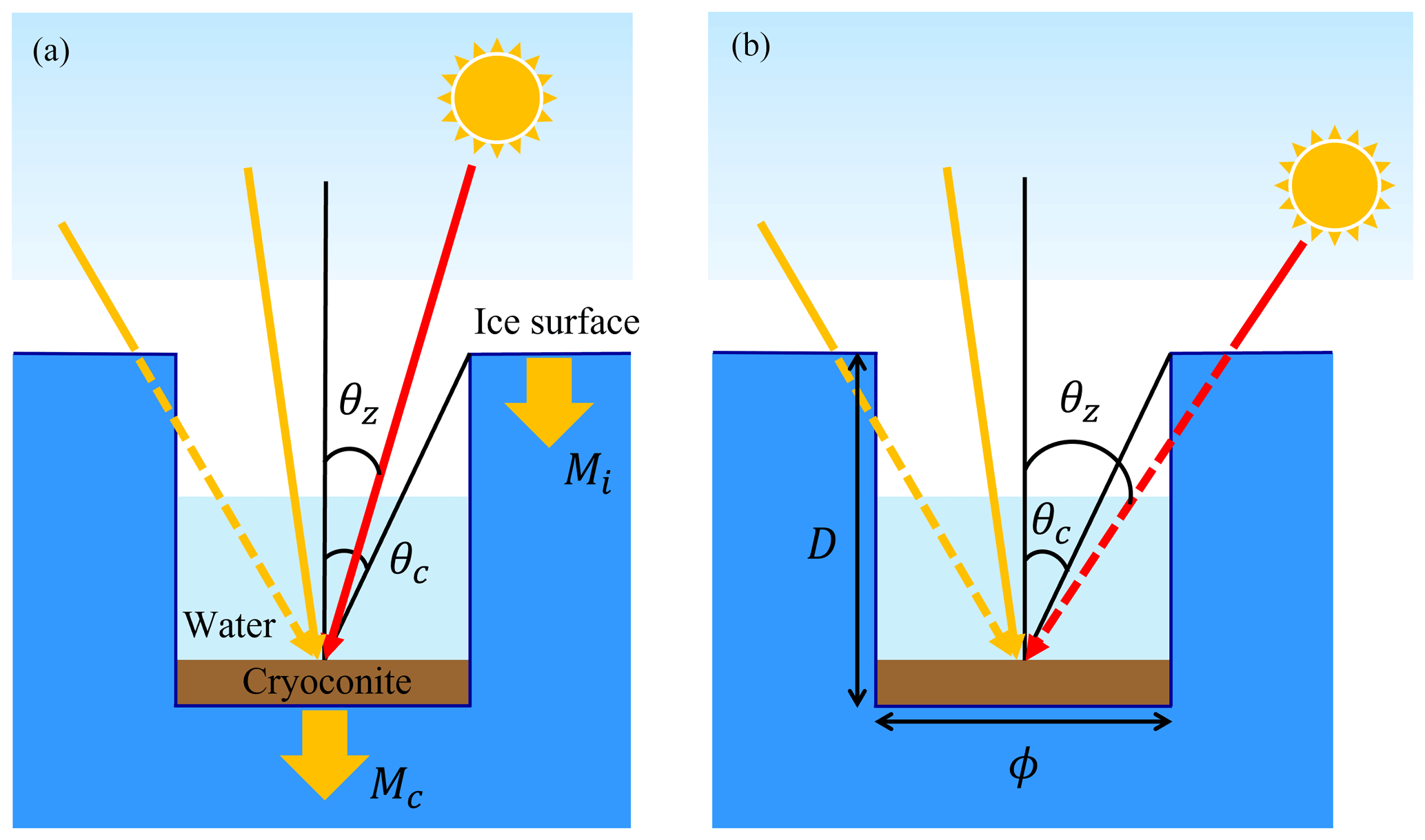
Figure 1 Concept of the cryoconite hole model (CryHo). Heat balances at the surface and cryoconite hole bottom are independently calculated (a). Red and orange arrows indicate direct and diffuse components of shortwave radiation, respectively. Cryoconite hole (CH) geometry, with depth (D) and diameter (ϕ) being considered for distinguishing the direct component of shortwave radiation (a). Cryoconite thickness at the CH bottom is assumed to be zero in the model. The difference between melting ice thickness at the surface (M_i) and that at the CH bottom (M_c) changes the CH depth. The direct component of solar radiation can reach the CH bottom from the hole mouth if the solar zenith angle θ_z is smaller than the zenith angle of the CH edge θ_c (a, solid red arrow), while it is transmitted through the ice if the solar zenith angle is greater than the zenith angle of the CH edge (b, dashed red arrow). The diffuse component of downward shortwave radiation can reach the CH bottom regardless of θ_z (solid and dashed orange arrows).

Table 1 Variables and constants used in this study. Variables that have different surfaces are indicated by a subscript (see footnote below the table for more information). i indicates the ice surface, and c indicates the cryoconite hole (CH) bottom.

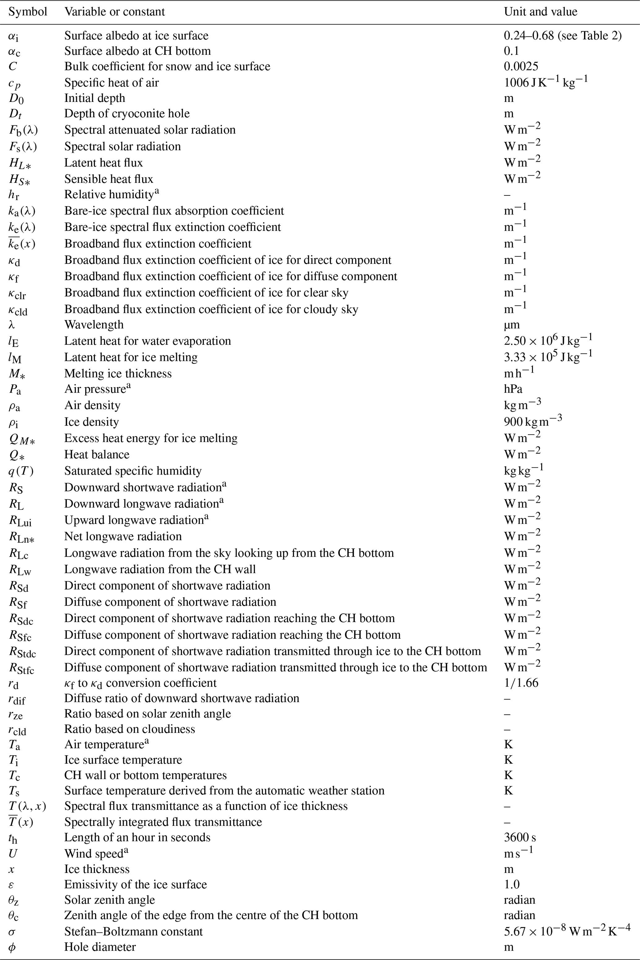
^a Denotes the input data for the cryoconite hole model (CryHo).

2 Cryoconite hole model (CryHo)

The cryoconite hole model (hereafter referred to as CryHo) developed in this study calculates the heat balances and resultant melt rates at the ice surface and CH bottom independently (Fig. 1). All variables and constants described in the following equations are listed in Table 1.

2.1 Heat balance at the ice surface

The heat balance at the ice surface (Q_i, W m⁻²) is described as follows:

$$\begin{array}{}\text{(1)}& {\displaystyle }& {\displaystyle }{Q}_{\mathrm{i}}=(\mathrm{1}-{\mathit{\alpha }}_{\mathrm{i}})R_{\mathrm{S}}+R_{\text{Lni}}+H_{\text{Si}}+H_{\text{Li}},\text{(2)}& {\displaystyle }& {\displaystyle }{R}_{\text{Lni}}=\mathit{\epsilon }{R}_{\mathrm{L}}-\mathit{\epsilon }\mathit{\sigma }{T}_{\mathrm{i}}^{\mathrm{4}},\end{array}$$

where α_i is the ice surface albedo (dimensionless); R_S s the downward shortwave radiation (W m⁻²); R_Lni is the net longwave radiation (W m⁻²); H_Si is the sensible heat flux (W m⁻²),; H_Li is the latent heat flux (W m⁻²); ε is the emissivity of the snow and ice surface, which is assumed to be 1.0 (dimensionless); R_L is the downward longwave radiation (W m⁻²); σ is the Stefan–Boltzmann constant (5.67 × 10⁻⁸ $\mathrm{W}{\mathrm{m}}^{-\mathrm{2}}{\mathrm{K}}^{-\mathrm{4}}$); and T_i is the surface temperature (K). Subscript i used in the variables refers to the ice surface. All the downward components have positive signs. Note that H_Li is restricted to the latent heat of evaporation; it does not include the latent heat of melting. Heat conduction from or toward the glacier ice and heat supplied by rainwater are assumed to be negligible. The turbulent heat fluxes (i.e. H_Si and H_Li) were estimated using the following bulk formulations:

$$\begin{array}{}\text{(3)}& {\displaystyle }& {\displaystyle }{H}_{\text{Si}}=c_p{\mathit{\rho }}_{\mathrm{a}}CU(T_{\mathrm{a}}-T_{\mathrm{i}}),\text{(4)}& {\displaystyle }& {\displaystyle }{H}_{\text{Li}}=l_{\mathrm{E}}{\mathit{\rho }}_{\mathrm{a}}CU\left(h_{\mathrm{r}}q\right(T_{\mathrm{a}})-q(T_{\mathrm{i}}\left)\right),\end{array}$$

where c_p is the specific heat of air (1006 $\mathrm{J}{\mathrm{K}}^{-\mathrm{1}}{\mathrm{kg}}^{-\mathrm{1}}$), ρ_a is the air density (kg m⁻³), C is the bulk coefficient for the snow and ice surface (0.0025, Kondo, 1994), U is the wind speed (m s⁻¹), T_a is the air temperature (K), l_E is the latent heat of water evaporation (2.50 × 10⁶ J kg⁻¹), h_r is the relative humidity (dimensionless), and q(T) is the saturated specific humidity (kg kg⁻¹). The excess energy (Q_i > 0) is used to melt the ice at the surface, once the surface temperature reaches the melting point (273.15 K), and its hourly amount is obtained as follows:

$$\begin{array}{ll}\text{(5)}& {\displaystyle }& {\displaystyle }{Q}_{\text{Mi}}=\text{max}[\mathrm{0},Q_{\mathrm{i}}],{\displaystyle }& {\displaystyle }{M}_{\mathrm{i}}={\displaystyle \frac{t_{\mathrm{h}}{Q}_{\text{Mi}}}{l_{\mathrm{M}}{\mathit{\rho }}_{\mathrm{i}}}},\end{array}$$

where Q_Mi is the excess heat energy for ice melt (W m⁻²), M_i is the melting ice thickness (m h⁻¹), t_h is the length of an hour in seconds (3600 s), l_M is the latent heat of ice melt (3.33 × 10⁵ J kg⁻¹), and ρ_i is the ice density assumed equal to 900 kg m⁻³.

2.2 Heat balance at the cryoconite hole bottom

The heat balance and melt rate at the CH bottom (denoted by subscript c) are defined as follows:

$$\begin{array}{ll}\text{(6)}& {\displaystyle }& {\displaystyle }{Q}_{\mathrm{c}}=(\mathrm{1}-{\mathit{\alpha }}_{\mathrm{c}})(R_{\text{Sdc}}+R_{\text{Sfc}}+R_{\text{Stdc}}+R_{\text{Stfc}})+R_{\text{Lnc}},\text{(7)}& {\displaystyle }& {\displaystyle }{Q}_{\text{Mc}}=\text{max}[\mathrm{0},Q_{\mathrm{c}}],{\displaystyle }& {\displaystyle }{M}_{\mathrm{c}}={\displaystyle \frac{t_{\mathrm{h}}{Q}_{\text{Mc}}}{l_{\mathrm{M}}{\mathit{\rho }}_{\mathrm{i}}}},\end{array}$$

where Q_c is the heat balance at the bottom (W m⁻²), α_c is the albedo (dimensionless), R_Sdc and R_Sfc are the direct and diffuse components of shortwave radiation (W m⁻²), R_Stdc and R_Stfc are the direct and diffuse components of shortwave radiation transmitted through ice (W m⁻²), R_Lnc is the net longwave radiation (W m⁻²), Q_Mc is the excess heat energy for ice melt (W m⁻²), and M_c is the melting ice thickness (m h⁻¹). Because we assume that the CH is partially filled with water, the turbulent heat fluxes at the bottom of the CH (i.e. H_Sc and H_Lc) are assumed to be 0 in Eq. (6). The change in CH depth (D_t, m) at a given time (t) is defined as follows:

$$\begin{array}{}\text{(8)}& D_t=D_{t-\mathrm{1}}+(M_{\mathrm{c}}-M_{\mathrm{i}}),\end{array}$$

where D_t−1 is the CH depth at one time step before (m). If the melt rate at the CH bottom is greater than that at the ice surface (M_c>M_i), the CH depth deepens (and vice versa). The initial depth D₀ at t=0 in CryHo is a prescribed constant initial condition. For simplicity, we assume the heat balance at the centre of the CH bottom can represent that of the entire bottom.

2.3 Geometry effect on the radiation components

In earlier CH models (Gribbon, 1979; Jepsen et al., 2010; Cook, 2012), downward shortwave radiation is reduced exponentially with increasing CH depth. The novel aspect of our model is that it considers not only the CH depth but also the CH shape geometry. The direct and diffuse components of downward shortwave radiation and downward longwave radiation are also considered independently. Regarding downward shortwave radiation, we first separate the observed downward shortwave radiation into direct and diffuse components (R_Sd and R_Sf, W m⁻²) as follows:

$$\begin{array}{}\text{(9)}& {\displaystyle }& {\displaystyle }{R}_{\text{Sd}}=(\mathrm{1}-r_{\text{dif}})R_{\mathrm{S}},\text{(10)}& {\displaystyle }& {\displaystyle }{R}_{\text{Sf}}=r_{\text{dif}}{R}_{\mathrm{S}},\end{array}$$

where r_dif is the diffuse ratio of downward shortwave radiation (dimensionless; 0–1), which is calculated following Goudriaan (1977):

$$\begin{array}{}\text{(11)}& r_{\text{dif}}=r_{\text{ze}}+(\mathrm{1}-r_{\text{ze}})r_{\text{cld}},\end{array}$$

where r_ze is the ratio based on the zenith angle (dimensionless; 0–1) and r_cld is the ratio based on cloudiness (dimensionless; 0–1). Calculation of r_ze was performed following Goudriaan (1977), and calculation of r_cld was performed following Broeke et al. (2004) and Niwano et al. (2015):

$$\begin{array}{}\text{(12)}& {\displaystyle }& {\displaystyle }{r}_{\text{ze}}={\displaystyle \frac{\mathrm{0.0604}}{\text{max}[\mathrm{0.01},(\text{cos}{\mathit{\theta }}_{\mathrm{z}}-\mathrm{0.0223}\left)\right]}}+\mathrm{0.0683},\text{(13)}& {\displaystyle }& {\displaystyle }{r}_{\text{cld}}=\mathrm{1}-{\displaystyle \frac{R_{\text{Lni}}}{[\mathrm{1363.2}-\mathrm{5.4}{T}_{\mathrm{a}}]}},\end{array}$$

where θ_z is the solar zenith angle (radian).

The CH geometry is defined as the zenith angle of the edge from the centre of the CH bottom (θ_c, rad) as follows:

$$\begin{array}{}\text{(14)}& {\mathit{\theta }}_{\mathrm{c}}={\tan }^{-\mathrm{1}}\left({\displaystyle \frac{\mathit{\varphi }}{\mathrm{2}{D}_{t-\mathrm{1}}}}\right),\end{array}$$

where ϕ is the diameter of CH (m).

Compared with the solar zenith angle, the direct component of shortwave radiation from the sky looking up from the CH bottom (R_Sdc; W m⁻²) is calculated as follows:

$$\begin{array}{llll}\text{(15)}& {\displaystyle }& {\displaystyle }{R}_{\text{Sdc}}=R_{\text{Sd}}& {\displaystyle }& {\displaystyle }[\text{if }{\mathit{\theta }}_{\mathrm{z}}\le {\mathit{\theta }}_{\mathrm{c}}],{\displaystyle }& {\displaystyle }{R}_{\text{Sdc}}=\mathrm{0}& {\displaystyle }& {\displaystyle }[\text{if }{\mathit{\theta }}_{\mathrm{z}}>{\mathit{\theta }}_{\mathrm{c}}].\end{array}$$

Meanwhile, the diffuse component of shortwave radiation from the sky looking up from the CH bottom (R_Sfc, W m⁻²) is obtained as follows:

$$\begin{array}{}\text{(16)}& R_{\text{Sfc}}=\left(\mathrm{1}-{\text{cos}}^{\mathrm{2}}{\mathit{\theta }}_{\mathrm{c}}\right)R_{\text{Sf}}.\end{array}$$

Shortwave radiation components transmitted through ice are described in the following section.

Longwave radiation from the sky looking up from the CH bottom (R_Lc; W m⁻²) can be obtained in a manner similar to R_Sfc as follows:

$$\begin{array}{}\text{(17)}& R_{\text{Lc}}=\left(\mathrm{1}-{\text{cos}}^{\mathrm{2}}{\mathit{\theta }}_{\mathrm{c}}\right)\mathit{\epsilon }{R}_{\mathrm{L}}.\end{array}$$

Longwave radiation from the CH wall (R_Lw; W m⁻²) is subsequently described as follows:

$$\begin{array}{}\text{(18)}& R_{\text{Lw}}={\text{cos}}^{\mathrm{2}}{\mathit{\theta }}_{\mathrm{c}}\mathit{\epsilon }\mathit{\sigma }{T}_{\mathrm{c}}^{\mathrm{4}}.\end{array}$$

Here, we assume that the CH wall or bottom temperatures (T_c; K) are equal to the melting point. Because the CryHo does not calculate water level in the CH, the longwave radiation emitted from the CH wall is calculated using snow and ice surface emissivity, which is similar to the water emissivity in Eq. (18). Regarding longwave radiation emitted from the CH bottom, the net longwave radiation (R_Lnc; W m⁻²) can be summarized as follows:

$$\begin{array}{}\text{(19)}& R_{\text{Lnc}}=R_{\text{Lc}}+R_{\text{Lw}}-\mathit{\epsilon }\mathit{\sigma }{T}_{\mathrm{c}}^{\mathrm{4}}=\left(\mathrm{1}-{\text{cos}}^{\mathrm{2}}{\mathit{\theta }}_{\mathrm{c}}\right)R_{\text{Lni}}.\end{array}$$

2.4 Shortwave radiation transmitted through ice

Depending on whether direct solar radiation illuminates the CH bottom (θ_z≤θ_c) or not (θ_z>θ_c), the direct and diffuse components of shortwave radiation transmitted through the ice (R_Stdc and R_Stfc, W m⁻²) are described as follows:

$$\begin{array}{llll}\text{(20)}& {\displaystyle }& {\displaystyle }{R}_{\text{Stdc}}=e^{\frac{-{\mathit{\kappa }}_{\mathrm{d}}{D}_{t-\mathrm{1}}}{\text{cos}{\mathit{\theta }}_{\mathrm{z}}}}{R}_{\text{Sd}}& {\displaystyle }& {\displaystyle }[\text{if }{\mathit{\theta }}_{\mathrm{z}}>{\mathit{\theta }}_{\mathrm{c}}],{\displaystyle }& {\displaystyle }{R}_{\text{Stdc}}=\mathrm{0}& {\displaystyle }& {\displaystyle }[\text{if }{\mathit{\theta }}_{\mathrm{z}}\le {\mathit{\theta }}_{\mathrm{c}}],\\ \text{(21)}& {\displaystyle }& {\displaystyle }{R}_{\text{Stfc}}={\text{cos}}^{\mathrm{2}}{\mathit{\theta }}_{\mathrm{c}}{e}^{-{\mathit{\kappa }}_{\mathrm{f}}{D}_{t-\mathrm{1}}}{R}_{\text{Sf}},& {\displaystyle }& {\displaystyle }\end{array}$$

where κ_d and κ_f are the broadband asymptotic volume flux extinction coefficients (hereafter broadband flux extinction coefficients) of ice (m⁻¹) for the direct and diffuse components, respectively. For the direct component, the path length of the transmitted light is considered, whereas for the diffuse component, it is assumed to be the CH depth.

The broadband flux extinction coefficient for the diffuse component (κ_f) can be calculated from the spectral flux extinction coefficients. However, this is not a simple integration because the spectral distribution of shortwave radiation transmitted through the ice varies depending on both the solar illumination spectral distribution and the path length in the ice. Thus, we first calculate the insolation spectral distribution in the ice from both the spectral flux extinction coefficients experimentally determined by Cooper et al. (2021) for ice on the GrIS (the term “irradiance attenuation coefficient” was used in their study) and the spectral solar radiation at the ice surface assumed for clear and cloudy skies, computed using a radiative transfer model (Aoki et al., 1999; 2000).

2.4.1 Theoretical basis for calculating bare-ice broadband flux extinction coefficient

Section 2.4.1 presents an expression for the broadband asymptotic volume flux extinction coefficient, κ (m⁻¹), from the spectral asymptotic volume flux extinction coefficient k_e(λ) (m⁻¹) of bare ice, where λ is the wavelength (µm). In this study, we simply refer to them as the “broadband (or spectral) flux extinction coefficient.” When the bare ice surface is illuminated by the spectral solar radiation F_s(λ), the attenuated solar radiation F_b(λ) at ice thickness x (m) in bare ice is expressed by k_e(λ) as follows:

$$\begin{array}{}\text{(22)}& F_{\mathrm{b}}\left(\mathit{\lambda }\right)=F_{\mathrm{s}}\left(\mathit{\lambda }\right)\text{exp}[-k_{\mathrm{e}}(\mathit{\lambda }\left)x\right].\end{array}$$

Using Eq. (22), the spectral flux transmittance (T(λ,x); dimensionless) as a function of x is described as follows:

$$\begin{array}{}\text{(23)}& T(\mathit{\lambda },x)={\displaystyle \frac{F_{\mathrm{b}}\left(\mathit{\lambda }\right)}{F_{\mathrm{s}}\left(\mathit{\lambda }\right)}}=\text{exp}[-k_{\mathrm{e}}(\mathit{\lambda }\left)x\right].\end{array}$$

The spectrally integrated flux transmittance $\stackrel{\mathrm{‾}}{T}\left(x\right)$ is calculated from F_s(λ) and T(λ,x) as follows:

$$\begin{array}{}\text{(24)}& \stackrel{\mathrm{‾}}{T}\left(x\right)={\displaystyle \frac{{\int }_{\mathrm{0}}^{\mathrm{\infty }}{F}_{\mathrm{s}}\left(\mathit{\lambda }\right)T(\mathit{\lambda },x)\mathrm{d}\mathit{\lambda }}{{\int }_{\mathrm{0}}^{\mathrm{\infty }}{F}_{\mathrm{s}}\left(\mathit{\lambda }\right)\mathrm{d}\mathit{\lambda }}}.\end{array}$$

Using Eq. (24), the broadband flux extinction coefficient ($\stackrel{\mathrm{‾}}{k_{\mathrm{e}}}\left(x\right)$, m⁻¹) is described as follows:

$$\begin{array}{}\text{(25)}& \begin{array}{rl}\stackrel{\mathrm{‾}}{k_{\mathrm{e}}}\left(x\right)& ={\displaystyle \frac{-\text{ln}\left(\stackrel{\mathrm{‾}}{T}\right(x\left)\right)}{x}}\\ & =-\text{ln}\left({\displaystyle \frac{{\int }_{\mathrm{0}}^{\mathrm{\infty }}{F}_{\mathrm{s}}\left(\mathit{\lambda }\right)\text{exp}[-k_{\mathrm{e}}(\mathit{\lambda }\left)x\right]\mathrm{d}\mathit{\lambda }}{{\int }_{\mathrm{0}}^{\mathrm{\infty }}{F}_{\mathrm{s}}\left(\mathit{\lambda }\right)\mathrm{d}\mathit{\lambda }}}\right)/x.\end{array}\end{array}$$

2.4.2 Parameterization of broadband flux extinction coefficient

Using Eq. (25), we calculate the $\stackrel{\mathrm{‾}}{k_{\mathrm{e}}}\left(x\right)$ for bare ice in Greenland from the following two datasets for k_e(λ) and F_s(λ). The first dataset k_e(λ) is employed based on measurements by Cooper et al. (2021) for the bare ice “Layer A” and “Layer B”, which are defined as the ice layers at 12–77 and 53–124 cm depth, respectively. The second dataset F_s(λ) is theoretically simulated at λ = 0.24.0 µm with a spectral resolution of 0.025 µm using a radiative transfer model for the atmosphere–snow-and-ice system (Aoki et al., 1999, 2000), assuming clear- and cloudy-sky conditions in the subarctic model atmosphere over the bare ice surface. As the spectral range of k_e(λ) reported by Cooper et al. (2021) is limited around the visible wavelengths (λ = 0.35–0.75 µm), with their Table A1 data (λ = 0.35–0.60 µm) and the calculated values from their transmittance data (λ = 0.60–0.75 µm) being employed in this study, we assume k_e(λ) in the other spectral regions λ = 0.20.35 µm and λ = 0.754.0 µm by scaling the pure-ice spectral absorption coefficient k_a(λ) (Warren and Brandt, 2008) to connect to the values of Cooper et al. (2021), as shown in Fig. 2. It is inferred that the difference between the scaled k_e(λ) (pink curve) and pure-ice k_a(λ) (blue curve and red x symbols) is attributed to air bubbles in bare ice for λ ≥ 0.55 µm and impurities and air bubbles for λ < 0.55 µm from the discussion by Cooper et al. (2021). There are large uncertainties in k_a(λ) in λ = 0.35–0.75 µm, as shown by the blue curve (Warren and Brandt, 2008) and the red x symbols (Cooper et al., 2021) in Fig. 2. Regarding the scaled k_e(λ) validity in other spectral regions, we did not have verifiable data. In fact, the contribution to $\stackrel{\mathrm{‾}}{k_{\mathrm{e}}}\left(x\right)$ from k_e(λ) in the other spectral regions is very low. The simulated F_s(λ) for clear and cloudy skies for the solar zenith angle θ_z = 63.1^∘ is shown in Fig. S1 in the Supplement.

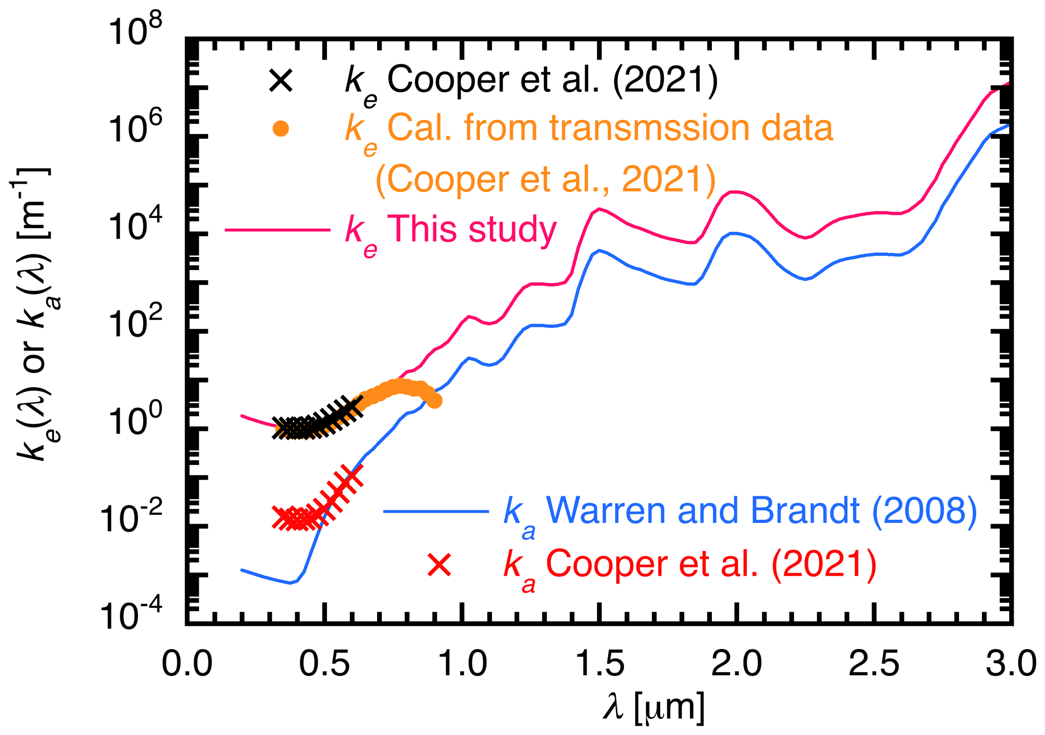
Figure 2 Spectral flux extinction coefficient (k_e(λ)) and absorption coefficient (k_a(λ)) in λ = 0.23.0 µm used for the calculation of $\stackrel{\mathrm{‾}}{k_{\mathrm{e}}}\left(x\right)$. k_e(λ) data for the wider spectral region in λ = 0.24.0 µm are used in the calculation of $\stackrel{\mathrm{‾}}{k_{\mathrm{e}}}\left(x\right)$. Black x symbols represent k_e(λ) reported by Cooper et al. (2021) for Layer A; orange dots represent k_e(λ) calculated from the transmittance data observed by Cooper et al. (2021); the pink curve is k_e(λ) used in this study; the blue curve is k_a(λ), calculated from the imaginary refractive index of pure ice (Warren and Brandt, 2008); and red x symbols represent k_a(λ) shown in Fig. S1 of Cooper et al. (2021) for Layer A, which is a reference for comparison with k_a(λ) of Warren and Brandt (2008).

Figure S2 demonstrates $\stackrel{\mathrm{‾}}{k_{\mathrm{e}}}\left(x\right)$ as a function of θ_z for x = 0.1 m calculated from k_e(λ) and F_s(λ) described above using Eq. (25). There is almost no difference in $\stackrel{\mathrm{‾}}{k_{\mathrm{e}}}\left(x\right)$ when we use k_e(λ) for layers A and B, as observed by Cooper et al. (2021). We also find that the θ_z dependence of $\stackrel{\mathrm{‾}}{k_{\mathrm{e}}}\left(x\right)$ is small in the range of θ_z from 50–86^∘, and thus we determine the θ_z-independent $\stackrel{\mathrm{‾}}{k_{\mathrm{e}}}\left(x\right)$ values by averaging it over this range of θ_z. By plotting the θ_z-independent values of $\stackrel{\mathrm{‾}}{k_{\mathrm{e}}}\left(x\right)$ as a function of x for clear and cloudy skies (Fig. 3), the $\stackrel{\mathrm{‾}}{k_{\mathrm{e}}}\left(x\right)$ values rapidly decrease in the shallower ice layer and change to a gentle slope in the deeper ice layer when x increases. This is because the spectral distribution of F_b(λ) in bare ice changes from a wider distribution to a narrower distribution centred around the minimum k_e(λ) wavelength, where the light absorption by bare ice is weakest as x increases. We can then obtain the approximation equations by fitting the calculated values of $\stackrel{\mathrm{‾}}{k_{\mathrm{e}}}\left(x\right)$ with a power regression equation, as shown in Table S1 in the Supplement. In this study, we use the terms “κ_clr” and “κ_cld” as the $\stackrel{\mathrm{‾}}{k_{\mathrm{e}}}\left(x\right)$ values for clear and cloudy skies, respectively. Finally, we determine the following approximation equations (Eqs. 26 and 27) of the broadband flux extinction coefficients as a function of ice thickness for clear (κ_clr; m⁻¹) and cloudy (κ_cld; m⁻¹) skies (Eq. 25 and Fig. 3).

$$\begin{array}{}\text{(26)}& {\displaystyle }& {\displaystyle }{\mathit{\kappa }}_{\text{clr}}=\mathrm{1.917}{D_{t-\mathrm{1}}}^{-\mathrm{0.613}},\text{(27)}& {\displaystyle }& {\displaystyle }{\mathit{\kappa }}_{\text{cld}}=\mathrm{1.620}{D_{t-\mathrm{1}}}^{-\mathrm{0.519}}.\end{array}$$

where κ_clr and κ_cld are calculated using the Layer A values shown in Table S1, as we focus on the vertical change in cryoconite holes below 0.20 m. The broadband flux extinction coefficient for the diffuse component (κ_f) is determined in a similar manner for the estimation of R_Sd and R_Sf as follows:

$$\begin{array}{}\text{(28)}& {\mathit{\kappa }}_{\mathrm{f}}=(\mathrm{1}-r_{\text{dif}}){\mathit{\kappa }}_{\text{clr}}+r_{\text{dif}}{\mathit{\kappa }}_{\text{cld}}.\end{array}$$

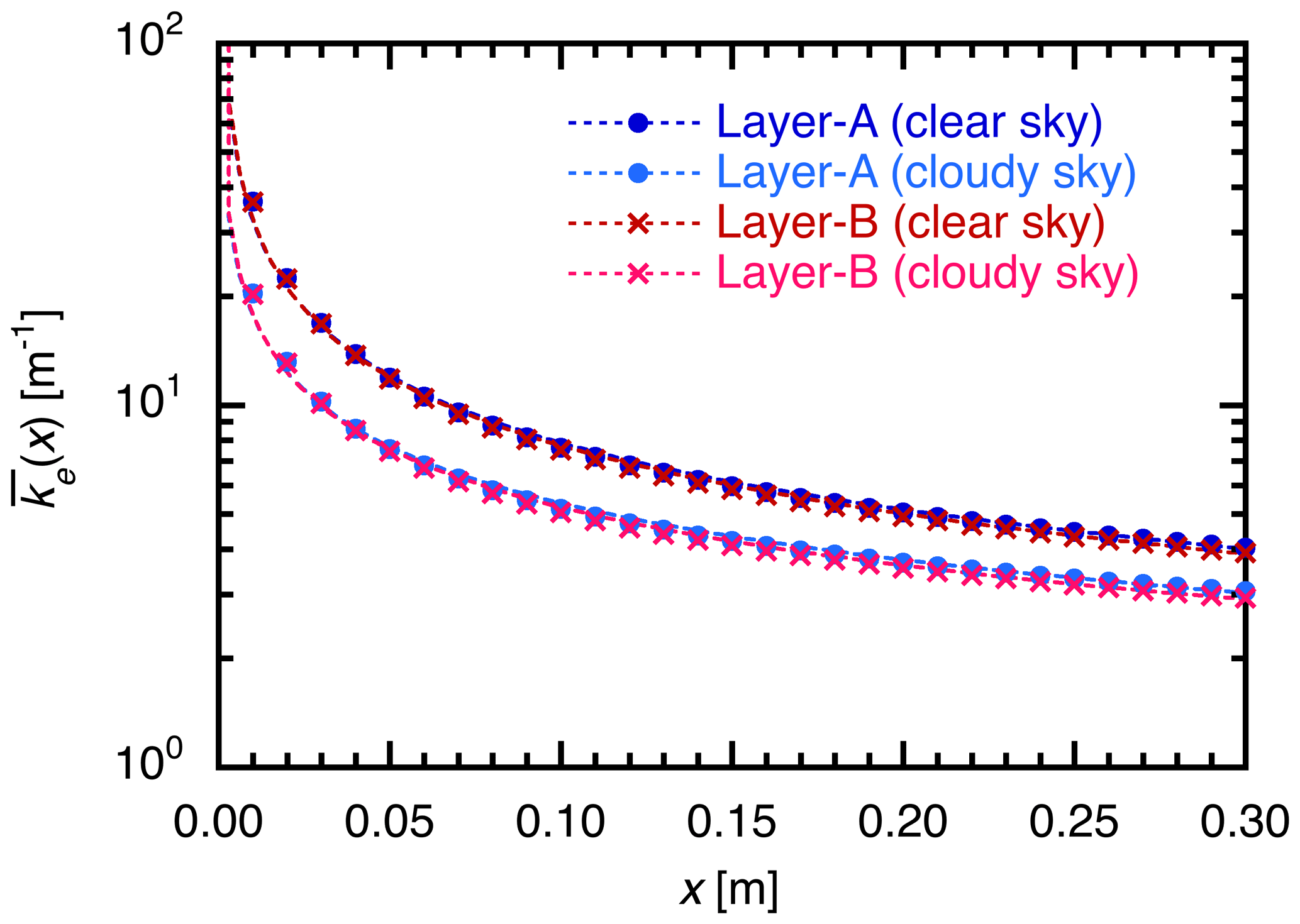
Figure 3 Broadband flux extinction coefficient $\stackrel{\mathrm{‾}}{k_{\mathrm{e}}}\left(x\right)$ of bare ice as a function of ice thickness x for clear- and cloudy-sky conditions and employed datasets of k_e(λ) for layers A and B reported by Cooper et al. (2021). Calculated values are indicated by symbols, and dashed curves represent approximation equations fitted by power regression equations.

As there are no available data for estimating the extinction coefficient for the direct component (κ_d), we parameterize it by introducing a coefficient (r_d) as follows:

$$\begin{array}{}\text{(29)}& {\mathit{\kappa }}_{\mathrm{d}}=r_{\mathrm{d}}{\mathit{\kappa }}_{\mathrm{f}}.\end{array}$$

The coefficient r_d was assumed to be $\mathrm{1}/\mathrm{1.66}$. The value 1.66 is used as an approximation value of the effective optical path length when the transmittance of the diffuse component of shortwave radiation is obtained from that of the direct component of shortwave radiation (Liou, 1980). Because we first estimate the diffuse component coefficient, κ_d was obtained by dividing κ_f by 1.66.

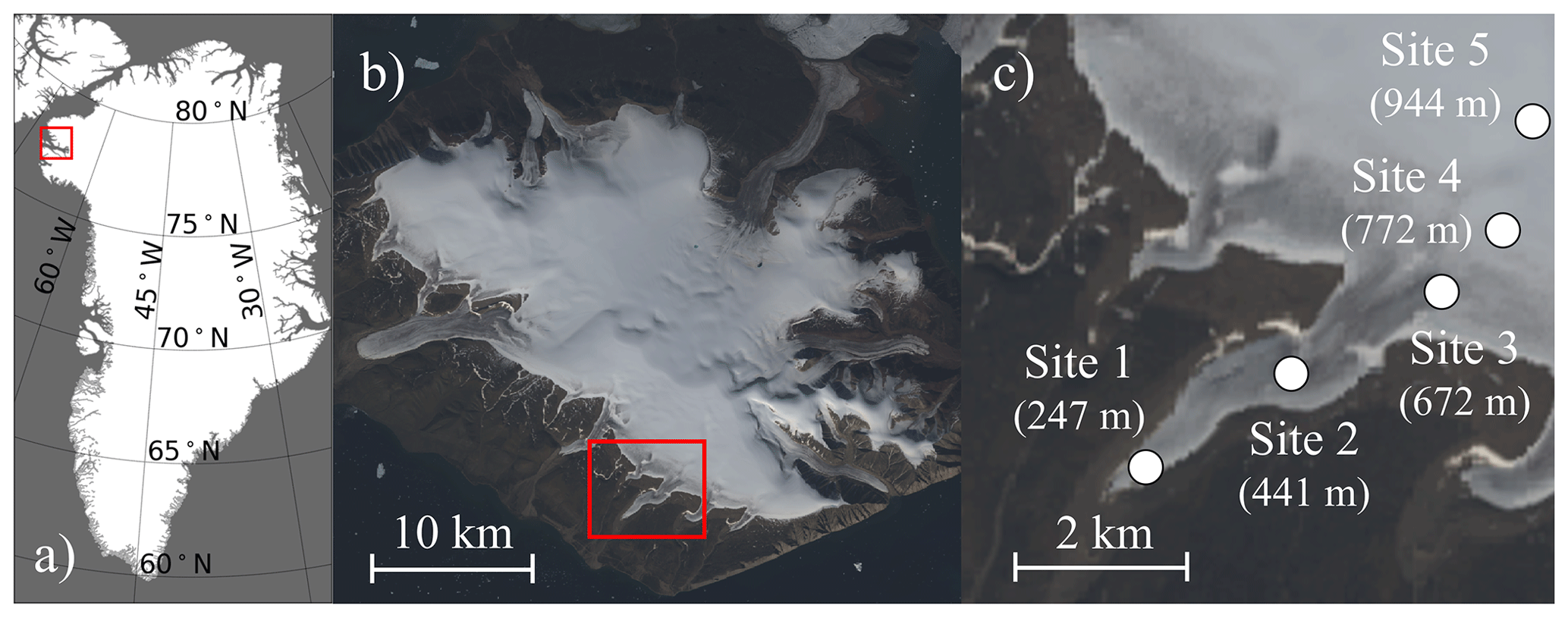
Figure 4 (a) Map of Greenland, (b) Qaanaaq ice cap in northwestern Greenland, and (c) study sites along the Qaanaaq Glacier. Panels (b) and (c) are true-colour composite images of Sentinel-2 taken on 24 July 2017. Red rectangles in panels (a) and (b) indicate the Qaanaaq area and Qaanaaq Glacier, respectively.

3 Observations

3.1 Site location

To evaluate the model, we investigated changes in CH depth at the Qaanaaq ice cap in northwestern Greenland (Fig. 4) during the 2012, 2014, and 2017 summer seasons. The ice cap covers an area of 286 km² and has an elevation range of 0–1200 $\mathrm{m}\mathrm{a}.\mathrm{s}.\mathrm{l}.$ (Sugiyama et al., 2014). We selected five study sites at different elevations (sites 1 to 5) on the Qaanaaq Glacier, which is an outlet glacier of the ice cap that is easily accessible from Qaanaaq village. Sites 1 to 5 are located in the middle of the glacier at elevations of 247, 441, 672, 772, and 944 $\mathrm{m}\mathrm{a}.\mathrm{s}.\mathrm{l}.$, respectively. The equilibrium line elevation of the glacier ranged between 862 and 1,001 $\mathrm{m}\mathrm{a}.\mathrm{s}.\mathrm{l}.$ in early August 2012, 2014, and 2017 (Tsutaki et al., 2017); hence, the ice surfaces at sites 1 to 5 were exposed during the ablation period from July to August.

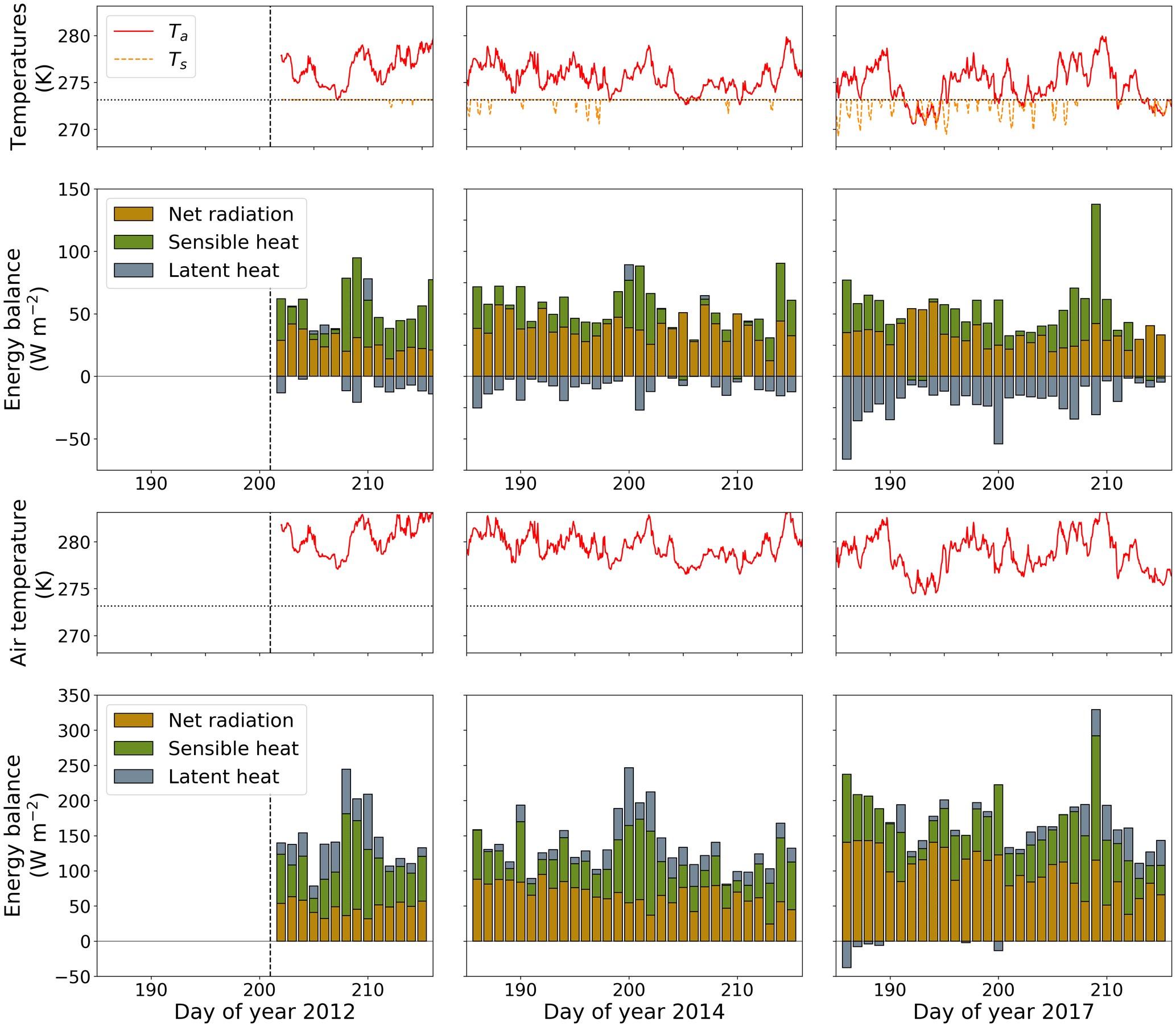
Figure 5 (a) Hourly air and surface temperatures (T_a and T_s in the upper panels, respectively) and daily surface energy balance (lower panels) at the Sigma-B site (Site 5 in this study) on the Qaanaaq ice cap during the 2012, 2014, and 2017 summer seasons from left to right, respectively. (b) Hourly air temperature (upper panels) and daily surface energy balance (lower panels) at Site 2. T_s shown in the upper panels in (a) is calculated from the downward and upward longwave radiation. T_a shown in the upper panels in (b) is corrected from T_a in (a) and an observed lapse rate. Dotted lines in the upper panels indicate the melting point (273.15 K). Daily surface energy balance is calculated with CryHo. The individual energy flux positive signs show a downward component.

3.2 Observations of meteorological variables and surface reflectance

The meteorological data that were used as input in CryHo were collected with an automatic weather station (AWS), which was established at the SIGMA-B site (77.518^∘ N, 69.0619^∘ W; 944 $\mathrm{m}\mathrm{a}.\mathrm{s}.\mathrm{l}.$), i.e. at Site 5 in this study, on 19 July 2012 (Aoki et al., 2014; Nishimura et al., 2021). Hourly air temperature (T_a; K), relative humidity (h_r; dimensionless), downward shortwave radiation (R_S; W m⁻²), downward longwave radiation (R_L; W m⁻²), upward longwave radiation (R_Lui; W m⁻²), wind speed (U; m s⁻¹), and air pressure (P_a; hPa) were collected for the model simulations described in Sect. 4. The seasonal changes in the measured air and surface temperatures and the calculated daily surface energy balance during the three studied summer seasons are shown in Fig. 5. The air and surface temperatures support the assumption that all study sites below the SIGMA-B site (i.e. Site 5) were mostly in ablation conditions during the three studied summer seasons. The heat balance was similar across the study years.

Table 2 Descriptions of cryoconite holes (CH) and ice surface reflectance at the study sites in 2012, 2014, and 2017. CH depths and diameters were observed using a ruler.

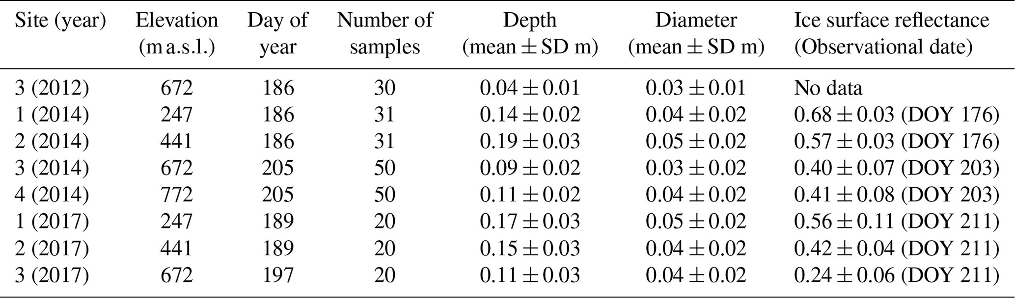
To determine the ice surface albedo used as input in CryHo, we measured the spectral reflectance from the visible to near-infrared band (0.350–1.050 µm) on the ice surface using a spectrometer (MS-720, Eiko Seiki Co., Japan) at the study sites during the 2014 and 2017 summer seasons (Table 2). For details on the observation method, we refer to Takeuchi et al. (2015). Although the mean reflectance differs optically from broadband albedo (0.300–3.000 µm), the reflectance measured at Site 3 in 2014 agrees well with the broadband albedo at the same site measured in 2012 (0.4 versus approximately 0.4; Takeuchi et al., 2018). Therefore, we assume that the reflectance shown in Table 2 can be used as a proxy for broadband albedo at the study sites for numerical simulations.

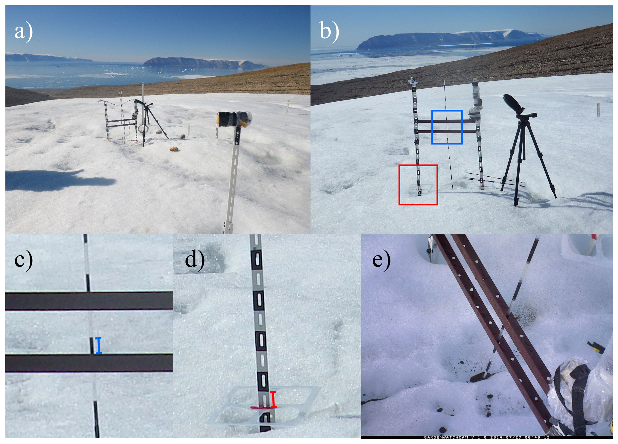
Figure 6 (a) Device for monitoring the cryoconite hole (CH) depth at Site 2. (b) Sample image to quantify the CH depth, which was taken by the interval camera (PENTAX WG-10) on day-of-the-year (DOY) 186 in 2014. (c) Close-up of the image within the blue rectangle in panel (b). (d) Close-up of the image within the red rectangle in panel (b). (e) CH conditions monitored by the interval camera (GardenWatch Cam) on DOY 208 in 2014. Blue and red bars in panels (c) and (d) indicate measured lengths to estimate the vertical changes in CH bottom and ice surface, respectively. Because the ice surface was uneven, the ice surface level was inferred based on the red tape pasted on the clear plastic frame shown in panel (d).

3.3 Monitoring cryoconite hole depth

To collect in situ data that can be used for the evaluation of CryHo, the temporal changes in CH depth were observed using the monitoring device, which consisted of two time-lapse cameras as well as a plastic stick positioned in the centre of a CH, supported by metal angles buried to approximately 1.5 m depth in the ice body (Fig. 6a). The temporal changes in CH depth were derived from variations in the heights of the plastic stick and white metal angle (Fig. 6b–d). To measure the variations, we marked both the stick and angle with clear and black colours at 5 cm intervals. The stick and angle were used to estimate the melt rates at the CH bottoms and ice surface surrounding the CHs, respectively. The variations were measured from hourly images with a resolution of 4608 pixel by 2592 pixel captured by a time-lapse camera (PENTAX WG-10, RICOH Co., Japan) installed at 3 m from the marked stick and angle. The time-lapse camera was placed 1 m above the ice surface and orthogonally oriented to the ice surface. To maintain the camera at the same height from the ice surface, we adjusted the height regularly (i.e. every 5–10 d). To capture the CH collapse event and check whether the plastic stick remained positioned in the CH, we also monitored the CHs using hourly images with a resolution of 1280 pixel by 1022 pixel taken by another time-lapse camera (GardenWatch Cam, Brinno Co., Taiwan, Fig. 6b). The location of the device was selected to have a suite of characteristics broadly identical to those of the monitoring site in a previous study (Takeuchi et al., 2018) in terms of cryoconite loading, ice structure, and ice surface slope of ∼ 5^∘. Monitoring was conducted from day-of-the-year (DOY) 194 to 214 in 2014.

To estimate the CH depths, the images were processed using ImageJ (version 1.48, National Institutes of Health, USA; Schneider et al., 2012). The CH depths were measured as relative variations using the length of marks on the stick for the CH bottom (Fig. 6c) and on the angle for the ice surface (Fig. 6d). One pixel corresponds to approximately 1 mm. Because the monitored CH collapsed between DOY 202 and 204, the sticks and angles were re-installed into another CH on DOY 205 (Fig. 6e).

Camera-based observations were conducted at Site 2, near the site where CH collapse occurred in 2012 (Takeuchi et al., 2018). We also conducted manual measurements of the depth and diameter of CHs two to four times during the 2014 and 2017 summer seasons. In addition, we used the dates of the CH collapse events reported by Takeuchi et al. (2018) for model evaluation. CH depths and diameters were manually measured from 20 to 50 randomly selected CHs at each site. Averages and standard deviations of the observed depths and diameters are summarized in Table 2.

4 Experimental design of the model evaluation and sensitivity tests

To evaluate CryHo, numerical simulations of the CH depth were conducted at several sites of the Qaanaaq ice cap for the three summer seasons (Site−exp). The number of study sites in 2012, 2014, and 2017 were 1 (Site 3), 4 (sites 1 to 4), and 3 (sites 1 to 3), respectively. The depths and diameters observed on the first observational date were used to set the model constants at each site (D₀ and ϕ in Table 2). The meteorological data measured at Site 5 were used as input for the simulations. At each site, T_a was corrected based on the air temperature measured at Site 5 and a temperature lapse rate of 7.80 × 10⁻³ K m⁻¹, which had been previously estimated from field observations on the same glacier in 2012 (Sugiyama et al., 2014). The other meteorological data at each site were assumed to be the same as those measured at Site 5. The observed surface temperature at Site 5 was almost the melting point during the three observational periods; thus, it was safely also used as input for the other sites, since they were located at lower elevations than that of Site 5 (Fig. 5a). In 2014, α_i at sites 1, 2, 3, and 4 was assumed to be 0.68, 0.57, 0.40, and 0.41, respectively (Table 2), as mentioned in Sect. 3.2. Similarly, in 2017, α_i at sites 1, 2, and 3 was assumed to be 0.56, 0.42, and 0.24, respectively (Table 2). α_i in 2012 for Site 3 was assumed to be 0.4, as observed by Takeuchi et al. (2018). We assumed the albedo at the CH bottom (α_c) to be 0.1 based on assumptions and observations in previous studies (e.g. Takeuchi et al., 2001; Jepsen et al., 2010). The calculation periods for the simulations in 2014 and 2017 were taken from the first date when CH depths were measured in June or July. In the 2012 simulation, the period was constrained by both CH and AWS observations.

Table 3 Overview of the sensitivity tests. Changing ranges for each variable are assumed based on the field observations in this study. Units of θ_z and θ_c in this table are converted to degrees for clarity.

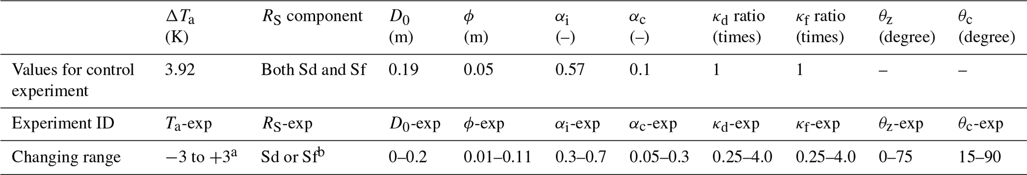
^a Change from the control experiment. ^b Shortwave radiation assumed to be only direct or diffuse component.

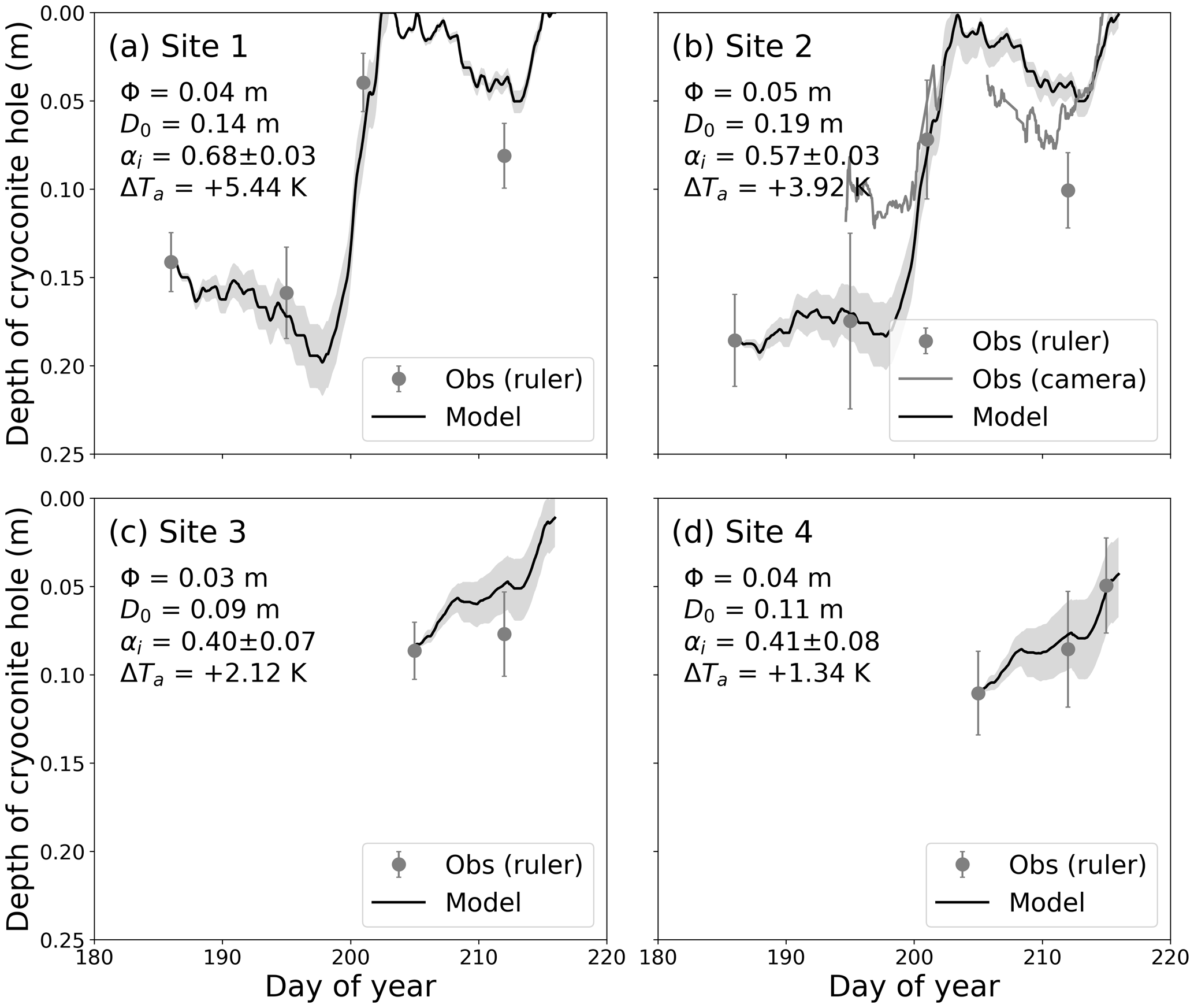
Figure 7 Temporal changes in cryoconite hole (CH) depth at (a) Site 1, (b) Site 2, (c) Site 3, and (d) Site 4 in 2014. The CH constants, ice surface albedo, and air temperature correction are described in each panel. The solid black line and shading indicate model results using average values and standard deviations of ice surface reflectance, which is assumed to be α_i, as shown in Table 2. The missing solid grey line in panel (b) denotes the CH collapse period.

We conducted sensitivity tests to assess the sensitivity of the CH depth to input data and model constants, such as air temperature (T_a-exp), radiation components (R_S-exp), initial depth (D₀-exp), hole diameter (ϕ-exp), albedo at the ice surface (α_i-exp), albedo at the CH bottom (α_c-exp), extinction coefficients of direct (κ_d-exp) and diffuse (κ_f-exp) radiation, solar zenith angle (θ_z-exp), and zenith angle of the edge from the centre of the CH bottom (θ_c-exp) (Table 3). Site−exp, i.e. Site 2 in 2014, was used as the control experiment for the sensitivity tests (Ctl−exp). The ranges of the changing parameters, which are summarized in Table 3, were determined based on field measurements (Table 2). The extinction coefficients for κ_d-exp and κ_f-exp were obtained from multiplying the original values by factors of 0.25–4.00. The factor range was assumed by referring to the difference between the spectral flux extinction coefficient and absorption coefficient calculated from the imaginary refractive index of pure ice (Fig. 2). In R_S-exp, we assumed r_dif of Eqs. (9) and (10) to be 0 and 1 in Sd and Sf cases shown in Table 3, respectively. Because we did not consider the light refraction at the air–water surface in the CH, we evaluated the refraction effect via sensitivity analysis (θ_z-exp) using various incident angles (θ_z). Although the heat balance at the CH bottom should vary across the width of the hole, particularly between the northern and southern edges, we assumed heat balance only at the centre of the CH bottom for the model simulation. The effect of different edges is evaluated by changing θ_c (θ_c-exp). In θ_z-exp and θ_c-exp, θ_z and θ_c calculated in the model were replaced with the values shown in Table 3, respectively.

To quantify the four components of shortwave radiation reaching the CH bottom (R_Sdc, R_Sfc, R_Stdc, and R_Stfc) for different CH geometries (i.e. depths and diameters), we conducted two sensitivity tests (R_ScD-exp and R_Scϕ-exp, respectively) at 13:00 and 01:00 LT (local time) on DOY 172 (i.e. the time of meridian transit and midnight at the summer solstice) in 2014. The CH depth and diameter ranged from 0.01 to 0.35 m in R_ScD-exp and from 0.01 to 0.15 m in R_Scϕ-exp, respectively. The CH diameter and depth were assumed to be 0.05 m in R_ScD-exp and 0.01 m in R_Scϕ-exp, respectively. The other model constants were the same as those in Ctl−exp.

To discuss the meteorological factors controlling the CH dynamics, besides the sensitivity tests described above, we also investigated the relationships between the CH deepening or shallowing rates against the input meteorological conditions, and the simulated heat properties at the ice surface at the CH bottom. These relationships were obtained from the input and output data in Ctl−exp. The deepening (shallowing) rate (m h⁻¹) was calculated when a CH deepened (shallowed) compared to its state 1 h earlier.

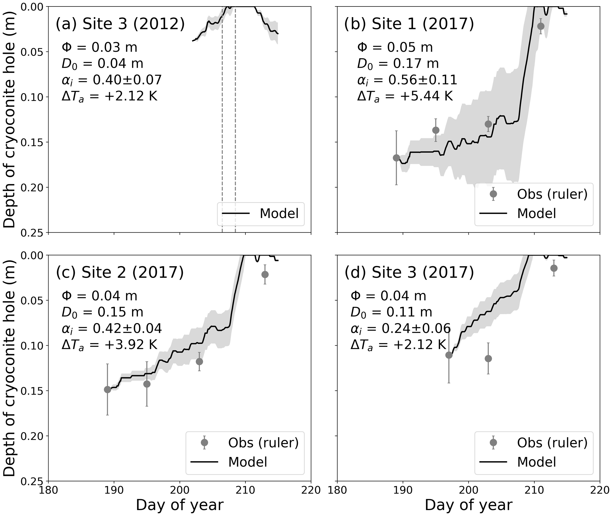
Figure 8 Temporal changes in cryoconite hole (CH) depth at (a) Site 3 in 2012, (b) Site 1 in 2017, (c) Site 2 in 2017, and (d) Site 3 in 2017. The CH constants and air temperature correction are described in each panel. The solid black line and shading indicate model results using average values and standard deviations of ice surface reflectance, which is assumed to be α_i, as shown in Table 2. Dashed grey lines in panel (a) indicate the collapse dates reported by Takeuchi et al. (2018).

5 Results and discussion

5.1 Evaluation of the cryoconite hole depth

The CH depth simulations at the different elevation sites in the 3 years (Site−exp) showed that the simulated temporal changes in CH depth, including CH collapse, agreed well with those observed at all sites for the 3 years (Figs. 7 and 8). The CH depth observed by both the camera and manual measurements at Site 2 gradually shallowed from DOY 186 to 202, developed until DOY 212, and shallowed again until DOY 215 (Fig. 7b). The modelled and camera-based CH depths at this site were in good agreement with each other (R² = 0.78; root-mean-square error of 0.04 m). In addition, the model also simulated the CH collapse event between DOY 202 and 204, during which the camera-based CH depth was not recorded (line gap in Fig. 7b). The model simulations revealed the good performance of the model also at the other sites (Fig. 7a, c, and d). Although no CH depth measurement was conducted in 2012, the model captured the CH collapses observed at Site 3 on DOY 206 and 208 (Fig. 8a, dashed grey lines). The manual measurements in 2017 showed similar temporal changes in CH depth to those in 2014 (Fig. 8b–d), which were also well represented by the model, especially the timing of drastic CH decay around DOY 210 at all sites. Because CryHo diagnoses the CH depth based on the balance between melt at the ice surface (M_i) and at the CH bottom (M_c), the model can capture the CH decay dynamics, which have not been simulated by previous numerical models considering only M_c (Gribbon, 1979; Jepsen et al., 2010; Cook, 2012). This indicates that the concept of CryHo, in which both heat balances (i.e. Q_i and Q_c) control the temporal change in the development and decay of CHs, is essentially correct. In the next section, we discuss the meteorological and/or ice physical factors that are important for simulating temporal changes in detail.

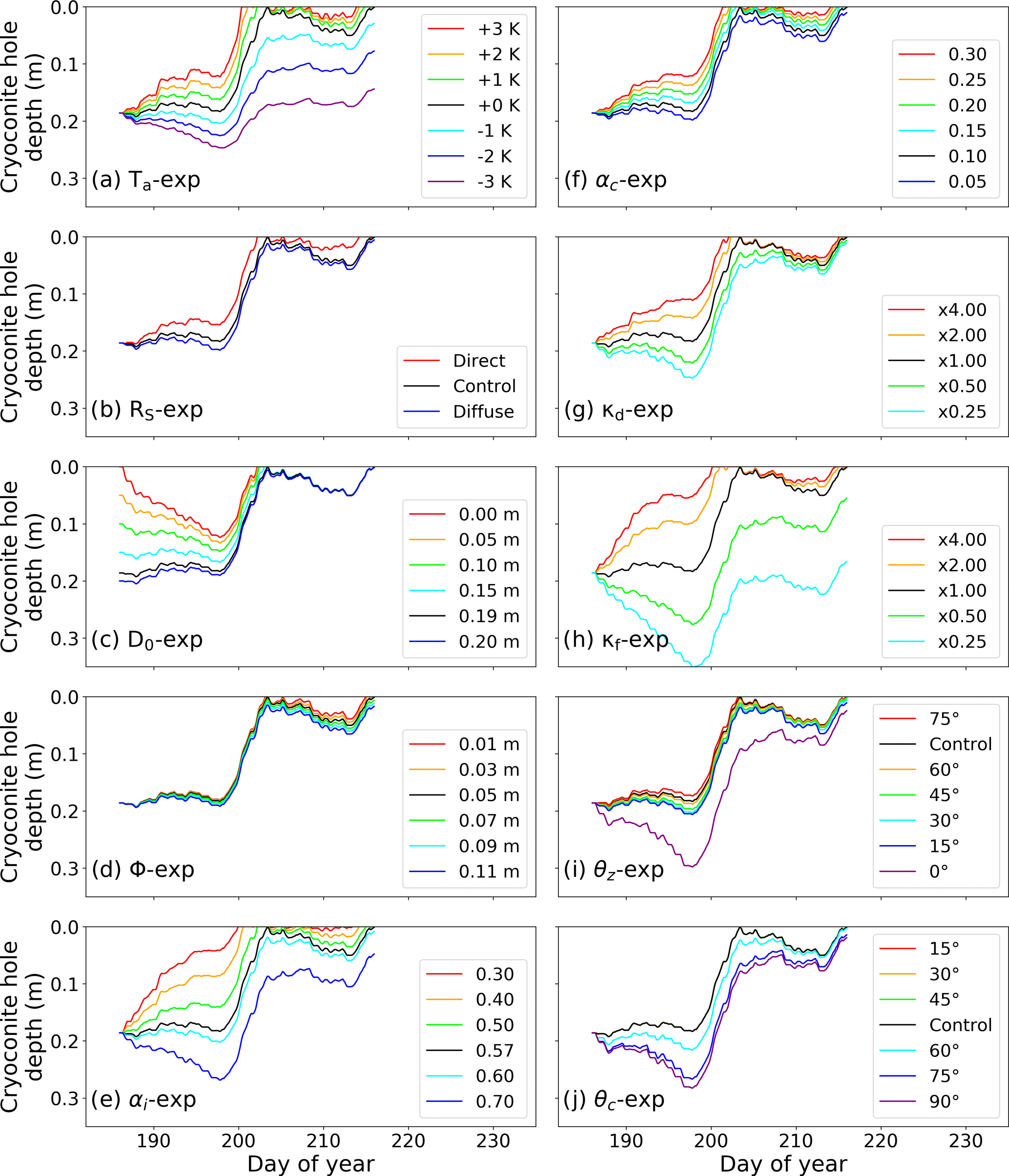
Figure 9 Sensitivity experiments of the temporal changes in cryoconite hole (CH) depth to model parameters and meteorological conditions at Site 2 in 2014. (a) Air temperature (T_a-exp), (b) shortwave radiation (R_S-exp), (c) initial CH depth (D₀-exp), (d) CH diameter (ϕ-exp), (e) ice surface albedo (α_i-exp), (f) cryoconite albedo (α_c-exp), broadband flux extinction coefficient of ice for the (g) direct component (κ_d-exp) and (h) diffuse component (κ_f-exp), (i) solar zenith angle (θ_z-exp), and (j) zenith angle of the edge from the centre of the CH bottom (θ_c-exp). Black lines in each figure indicate the control experiment (Ctl-exp). Note that lines for 15, 30, and 45^∘ in the bottom-right in (j) overlap with the line for control.

5.2 Sensitivity of the simulated hole depth to the model parameters

The sensitivity experiment regarding the air temperature (T_a-exp) suggests that CHs tend to be deeper and more stable under cooler conditions (and vice versa) (Fig. 9a). This is likely because the turbulent heat fluxes on the ice surface decrease under cooler conditions; thus, net radiation becomes the main component for ice melting, which is constrained by the albedo at the ice surface and CH bottom. Indeed, field observations indicated that the turbulent heat fluxes during warmer conditions (DOY 198–205) were increased compared to the case during cooler conditions (before DOY 198) at Site 2 in 2014 (Fig. 5b). Under such cooler conditions, the melt rate at the ice surface surrounding the CHs was lower, resulting in deeper and therefore more stable CHs. Indeed, Gribbon (1979) reported that the CH depth increased with the elevation of the glacier in western Greenland. Furthermore, higher melt rates (and hence warmer conditions) at the ice surface are likely to induce CH decay, as suggested by Hodson et al. (2007). Therefore, global warming may cause the collapse of CHs earlier in the melt season compared to the present case, thereby inducing darkening of the ice surface by cryoconite granule redistribution in the future. Nevertheless, a snow–ice–atmosphere coupling simulation using a climate model coupled with CryHo is necessary to evaluate the contribution of CH dynamics to surface darkening under climate change.

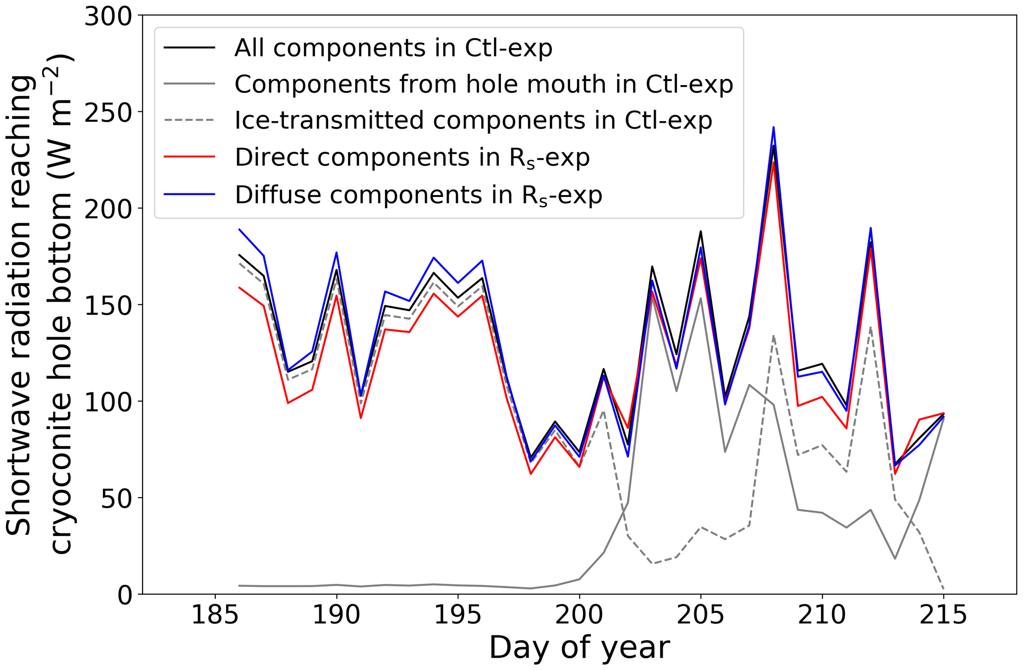
Figure 10 Daily mean temporal changes in direct and diffuse components of shortwave radiation reaching the cryoconite hole (CH) bottom in 2014. Blue and red lines indicate the direct (R_Sdt+R_Stdc) and diffuse (R_Sfct+R_Stfc) components in R_S-exp, respectively. The black line indicates both components of shortwave radiation ($R_{\text{Sdt}}+R_{\text{Sfct}}+R_{\text{Stdc}}+R_{\text{Stfc}}$) in Ctl−exp. Solid and dashed grey lines indicate the radiation components reaching the CH bottom from the hole mouth (R_Sdt+R_Stdc) and transmitting through ice (R_Sfct+R_Stfc) in Ctl−exp, respectively.

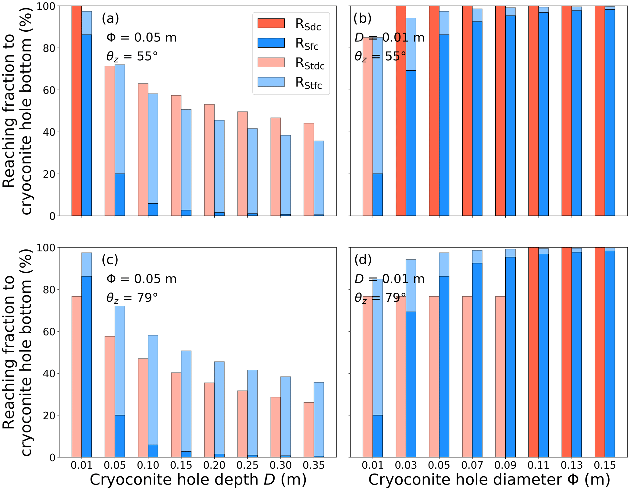
Figure 11 Sensitivity experiments of the cryoconite hole (CH) geometry on the direct and diffuse components of shortwave radiation reaching the CH bottom for (a, c) CH depth and (b, d) CH diameter. Dark red and blue bars in the figure indicate the direct and diffuse components of shortwave radiation, respectively. Light red and blue bars indicate the direct and diffuse components of shortwave radiation transmitted throughout ice, respectively. The vertical axis represents the fraction of direct and diffuse components against the incoming shortwave radiation at the ice surface (100 % at the ice surface). The ratios were derived from numerical simulations with different CH depth or CH diameter on day-of-the-year (DOY) 172 in 2014. The meteorological conditions for the simulations were assumed to be those at 13:00 (a, b) and 01:00 LT (c, d) on the date used for Ctl−exp.

The sensitivity experiment regarding the shortwave radiation components (R_S-exp) suggests that CHs tend to decay and develop when the direct and diffuse components, respectively, are dominant (Fig. 9b). We then compared the contributions of each radiation component reaching the CH bottom during the experimental period (Fig. 10, red and blue lines). The CH bottom is more accessible by the diffuse component (R_Sfc+R_Stfc) rather than the direct component (R_Sdc+R_Stdc), except for shallowing depth case. In the model, the direct component of shortwave radiation can reach the CH bottom only when the solar zenith angle θ_z is smaller than the CH edge θ_c (Fig. 1 and Eq. 15), and it is transmitted through the ice in the opposite case. Because θ_z and θ_c ranged from 56 to 85^∘ and 8 to 90^∘ during the simulation period at the studied glacier, respectively, the direct component reaching the CH bottom from the hole mouth was very limited. Figure 11a shows that there is no significant difference between the direct and diffuse components reaching the CH bottom even at the time of meridian transit in the summer solstice, suggesting that the diffuse component reaches the CH bottom more frequently than the direct component in the studied glacier. To investigate heat flux to the CH bottom by shortwave radiation from the hole mouth or through the ice, we additionally compared the contributions of each radiation component reaching the CH bottom (Fig. 10, grey lines). The figure shows that the radiation components transmitted through ice to the CH bottom (R_Stfc+R_Stdc) were greater than the radiation components reaching the CH bottom from the hole mouth (R_Sfc+R_Sdc) when CH developed from DOY 208 to 213, meaning that radiation components transmitted through ice are also important for the heat balance at the CH bottom (i.e. Q_c). Further discussion regarding shortwave radiation transmitted throughout the ice is described later.

The sensitivity experiments regarding the CH geometry (D₀-exp and ϕ-exp) suggest that differences in the geometrical parameters have little influence on the CH depth. The simulated CH depth starting from different initial depths converged within approximately 2 weeks (Fig. 9c). This is probably because the CH bottom is relatively accessible by shortwave radiation in the case of shallower depths (and vice versa) (Fig. 11), which is quantified by additional experiments (R_ScD-exp and R_Scϕ-exp). The diameter shows no significant effect on the CH depth (Fig. 9d), although it strongly affects whether shortwave radiation reaches the CH bottom. This is likely because transmitted shortwave radiation reaches the CH bottom irrespective of the CH diameter. Figure 11b suggests no significant difference in the total shortwave radiation reaching the CH bottom among the different diameters, thereby supporting the ϕ-exp result. Indeed, no significant correlation between the CH depth and diameter has been found (Gribbon, 1979; Cook, 2012). Because an increase in CH diameter allows more direct shortwave radiation to reach the CH bottom, positive feedback of the CH development is possible. However, such feedback is unlikely to occur because Fig. 11b and d suggest that most of the diffuse component of the transmitted shortwave radiation reaches the CH bottom at 0.01 m depth in CHs over 0.03 m in diameter. Furthermore, the observed CH depths and diameters significantly varied among the sites and years (Table 2), suggesting that CH depth is mainly controlled by factors other than the CH diameter.

The sensitivity experiments regarding the albedos of the ice surface and CH bottom (α_i-exp and α_c-exp) suggest that the difference between ice surface (α_i) and CH bottom albedo (α_c) is an important factor for reproducing the CH dynamics, especially the timing of CH collapse. The CH depth increases with an increase in α_i owing to decreasing M_i, whereas it decreases with an increase in α_c owing to decreasing M_c (Fig. 9e and f). Notably, the sensitivity of the CH depth to α_i was greater than that to α_c. This is probably because shortwave radiation at the ice surface was greater than that at the CH bottom. In addition, α_i-exp suggests that a 0.1 decrease in α_i induces CH collapse 1 d earlier. Although α_c is known to be a key parameter for simulating the CH deepening rate (Podgorny and Grenfell, 1996), there is little information and discussion regarding α_i. Because we used constant values of α_c and α_i in α_i-exp and α_c-exp, respectively, the CH depth sensitivity to the albedo is equivalent to the sensitivity difference between α_i and α_c. Therefore, our results first highlight the importance of the difference between α_i and α_c in simulating vertical CH variations in which CH tends to develop with greater albedo difference and vice versa. Furthermore, the collapse of CHs is likely to reduce the ice surface albedo, owing to the redistribution of cryoconite on the ice surface (Irvine-Fynn et al., 2011; Takeuchi et al., 2018). Considering studies that reported a darkening trend of the GrIS surface over the last 20 years (e.g. Shimada et al., 2016; Tedstone et al., 2017), a positive albedo feedback, during which a decrease in ice surface albedo causes frequent CH collapse events, may occur. While our assumed reflectance was based on the α_i observations in 2014, the ice surface albedo should change temporally. The uncertainty in the model simulations, such as that regarding the results around DOY 204 at Site 3 in 2017 (Fig. 8d), may be attributed to temporal changes in the ice surface albedo. To simulate the development and decay of CHs more accurately, temporal changes in the ice surface albedo, including the effects of CH collapse and algal blooms, should be incorporated into CryHo.

The sensitivity experiments regarding the broadband extinction coefficients of shortwave radiation transmitted throughout ice for the direct and diffuse components (κ_d-exp and κ_f-exp) suggest that κ_f is more effective at the CH depth than κ_d. Both experiments showed that the CH depth with a higher coefficient was shallower, owing to a decrease in M_c (Fig. 9g and h); however, there was a significant difference in the sensitivity to the coefficients. One reason is probably that κ_d is lower than κ_f, as in Eq. (29). Figure 10 showed that the diffuse component of shortwave radiation reaching the CH bottom was greater than the direct component of that even though κ_f is higher than κ_d, suggesting that the shortwave radiation diffuse component reaches the CH bottom more easily than the direct component. Indeed, Fig. 11 indicates that the reaching fraction of direct component of shortwave radiation transmitted throughout the ice to the CH bottom decreases with θ_z. This is probably the cause of the higher sensitivity to κ_f, suggesting that κ_f is likely a relatively more important parameter compared to κ_d. However, there was no significant difference in sensitivity between κ_f and κ_d in the case of θ_z≤θ_c, which is the case for depths shallower than approximately 0.50 m in Fig. 9g and h. In such a case, most of the direct and diffuse components reach the CH bottom without being transmitted through the ice (Fig. 11). Figure 11 also suggests that shortwave radiation transmitted throughout the ice is dominant in the opposite case. Since CH depth ranged from 0 to 0.20 m at Site 2 in 2014, the result supports our argument that transmitted shortwave radiation mainly contributes to CH development as described for R_S-exp. In the Antarctic, a lot of CHs of over 0.30 m depth were reported even though the CH mouths were covered with frozen ice (Fountain et al., 2004), suggesting that the contribution of the transmitted shortwave radiation to CH development is substantial. The results highlight the importance of separating the direct and diffuse components of shortwave radiation in CH depth simulations. Further studies of the optical characteristics of ice are necessary because there is little information on the broadband flux extinction coefficients. Furthermore, previous studies reported the development of a porous ice layer, known as the weathering crust, on glaciers worldwide during summer (Irvine-Fynn and Edwards, 2014; Stevens et al., 2022). The weathering crust density is sometimes less than 500 kg m⁻³ (Müller and Keeler, 1969). Because the shortwave radiation transmittance would be larger in a low-density case than that in the ice density case assumed in this study (900 kg m⁻³), CHs may also develop under the weathering crust. To accurately simulate temporal change in CH depth, more detailed surface ice properties, such as the weathering crust layer, should be considered for future CH modelling.

The sensitivity experiments regarding the zenith angle (θ_z-exp and θ_c-exp) suggest that differences in the zenith angles have little influence on CH depth, except for the instance in which the downward shortwave radiation always reaches the CH bottom from the hole mouth (θ_z = 0^∘). θ_z-exp showed that CH depth with a higher θ_z was shallower, owing to a decrease in M_c (Fig. 9i), and θ_c-exp showed that CH depth with a lower θ_c was also shallow (Fig. 9j). Notably, the experiments suggest that both θ_z and θ_c hardly affect CH depth at over 15^∘ and below 60^∘, respectively. Snell's law states that the direct component of incident radiation is refracted through the air–water surface. According to this law, the refraction angle is approximately 20^∘ smaller than the incident angle θ_z; therefore, the direct component of the downward shortwave radiation more easily reaches the CH bottom from the hole mouth. However, such refraction is unlikely to affect CH depth because θ_z is always greater than 55^∘ at the studied latitude. Although CryHo calculates M_c at the centre of the CH bottom using θ_c, M_c may differ at the northern and southern edges of the CH bottom because the zenith angles of the CH bottom edges would differ from θ_c. θ_c-exp suggests that CH depth is temporarily non-uniform on the northern and southern edges of the CH bottom. However, CH depth likely becomes uniform again over time according to D₀-exp. Indeed, the simulated CH depth using a different θ_c converged within approximately 2 weeks (Fig. 9j). A previous study suggests that the surface of the CH bottom on steep north-sloping ice is non-uniform due to heterogeneous radiation reaching the CH bottom (Cook et al., 2018). The slope in our studied sites is approximately 5^∘. The aspect in our studied sites is southwest. Thus, the surface of the CH bottom might remain uniform on such gentle south-sloping ice.

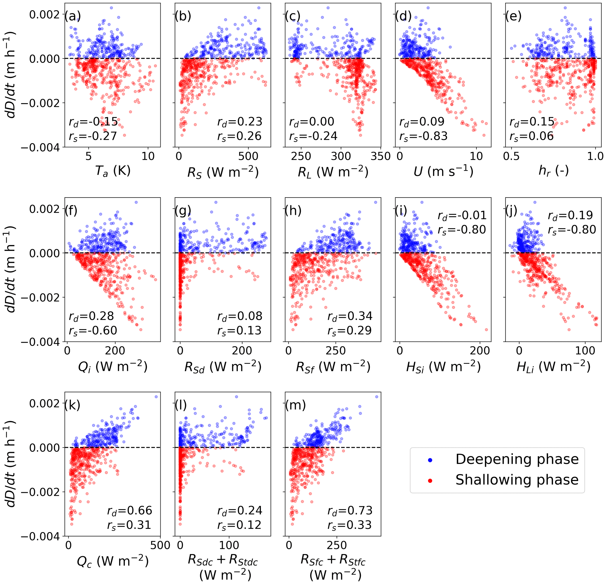
Figure 12 Relationships between the CH deepening or shallowing rates in the control experiment ($\mathrm{d}D/\mathrm{d}t$, m h⁻¹). The upper (a–e), middle (f–j), and bottom (k–m) panels indicate the relationships between the CH deepening or shallowing rates and the input meteorological conditions, simulated heat properties at the ice surface, and simulated heat properties at the CH bottom, respectively. Blue and red marks indicate the CH deepening and shallowing, respectively. Variables in the horizontal axis are shown in Table 1; r_d and r_s in each panel indicate the correlation coefficients with CH deepening and shallowing rates, respectively. Note that T_a in (a) is air temperature corrected for Site 2 where the control experiment was performed.

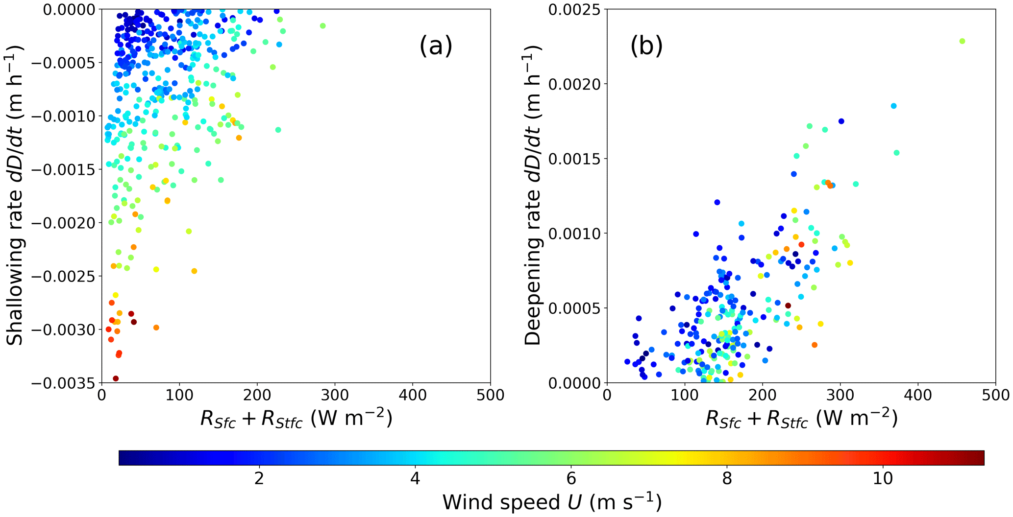
Figure 13 Relationships between the cryoconite hole (CH) (a) deepening or (b) shallowing rates and the diffuse component of downward shortwave radiation reaching the CH bottom and wind speed in the control experiment. The CH shallowing and deepening phases shown in Fig. 9m are separated into panels (a) and (b) in this figure, respectively. The contour in the panels indicates the input wind speed for the control experiment.

5.3 Meteorological factors controlling the cryoconite hole dynamics

The sensitivity tests in the previous section showed that CH depth did not equilibrate in any experimental cases at the studied glacier, where meteorological conditions change before the depth reaches equilibrium (Fig. 9). It suggests that meteorological conditions significantly affect CH depth. For example, downward shortwave radiation governs the CH deepening processes (Hodson et al., 2010a; Takeuchi et al., 2018). To better understand the factors controlling the CH deepening and shallowing processes, we compared the heat components with both the CH deepening and shallowing rates. In the shallowing phase (red marks in Fig. 12), CH decay is mainly controlled by the sensible and latent heat fluxes at the ice surface (H_Si and H_Li) via wind speed (U). Air temperature (T_a) shows no significant correlation with the shallowing rate; conversely, U shows a strong correlation with the shallowing rate (Fig. 12a and d). However, there is no clear relationship between the input downward shortwave radiation, input downward longwave radiation, relative humidity, and direct and diffuse components of downward shortwave radiation at the ice surface (R_S, R_L, h_r, R_Sd, and R_Sf shown in Fig. 12b, c, e, g, and h, respectively). The results suggest that strong winds induce CH decay by increasing the surface melt via the turbulent heat fluxes (Figs. 12f–j). Takeuchi et al. (2018) suggested that CHs tend to be shallower under both cloudy and windy conditions. Our analyses also suggest that windy conditions are important meteorological conditions governing the CH decay (Fig. 13a). Because the total downward shortwave is reduced through clouds, although the diffuse component of downward shortwave radiation generally increases under cloudy conditions, turbulent fluxes are likely to be dominant in the total energy budget, resulting in an ice surface that melts faster than the CH bottom. This is probably the reason why the CH collapse events were observed under cloudy conditions.

In the CH deepening phase (blue marks in Fig. 12), although the input shortwave radiation (R_S) was weakly correlated with the CH deepening rate, the diffuse component reaching the CH bottom was strongly correlated with the CH deepening rate (R_Sfc+R_Stfc), whereas no correlation was found with the direct component reaching the CH bottom (R_Sdc+R_Stdc) (Fig. 12l–m). Furthermore, Fig. 12k, which shows the relationship between ice melt at the CH bottom (Q_c) and the CH deepening rate, is similar to Fig. 12m. The results suggest an essential contribution of the diffuse component to CH development, which was also revealed by sensitivity analysis. However, the direct component strongly depends on the solar zenith angle and CH geometry (θ_z and θ_c); thus, the CH development is likely to be unstable during sunny conditions. Other meteorological variables are unlikely to contribute to the CH development. Although previous studies suggested that sunny conditions induce CH development (Hodson et al., 2010b; Irvine-Fynn et al., 2011; Takeuchi et al., 2018), our results highlight that the diffuse component of shortwave radiation is a key factor governing CH development, rather than merely sunny conditions. Because the CH deepening rate is likely to depend on wind speed and the intensity of the diffuse component of downward shortwave radiation, as shown in Fig. 13b, CHs could develop under sunny conditions depending on wind speed and other meteorological conditions. CH depths are mainly determined by the balance between the intensity of the diffuse component of downward shortwave radiation and the strength of the turbulent heat transfer.

5.4 Other possible factors affecting cryoconite hole dynamics

Our model does not include the effect of water lingering in CHs on the heat balance at the CH bottom because a quantitative understanding of the mechanism of convective heat transport or the buffering effect in the lingering water is insufficient. Such lingering water in CHs may affect the heat exchange between the atmosphere and CH bottom. Heat exchange should not be negligible in the case of large water surfaces in CHs. Although the water level in CHs is not estimated in the model, the refraction through the air–water surface in CHs is unlikely to affect CH depth in the studied glacier as discussed regarding θ_z-exp. However, such refraction might contribute to CH development in lower-latitude regions such as Asia, where the solar zenith angle is significantly smaller than that in the polar region. In addition to the refraction, reflectance at the water surface would reduce the amount of shortwave radiation reaching the CH bottom. To simulate CH depths globally, such an effect may need to be better incorporated into CryHo. Besides lingering water in CHs, the thickness of cryoconite at the CH bottom, which is not considered by CryHo, is also likely to be a key factor in determining the CH diameter and shape because a portion of the absorbed radiation in the cryoconite at the CH bottom could be transferred laterally and then melt the CH wall (Cook et al., 2010; Cook, 2012). Furthermore, the surface slope of the glacier affects the sediment thickness and thus the CH shape geometry via water flow and changes the shortwave radiation reaching the CHs (Takeuchi et al., 2000; Cook et al., 2018). Although such factors should be incorporated into CryHo in the future, CryHo is likely to reproduce the temporal change in CH depth well, even for relatively large CH on flat surfaces with diameters up to around 0.1 m, which falls within the range of CH shape geometries documented in this study. Compared to the effects of CH shape geometry and topological conditions, the effects of lingering water and sediment thickness in CHs on the CH depth may be small. The CH diameter range of 0.01 to 0.11 m assumed for ϕ-exp is similar to that observed in glaciers in western Greenland, Svalbard, and the Himalayas (Gribbon, 1979; Takeuchi et al., 2000; Cook et al., 2010), suggesting that CryHo can be applied also to these regions.

6 Conclusions

We established a numerical cryoconite hole model (CryHo) to reproduce the vertical cryoconite hole (CH) dynamics. We evaluated the model using field observations from an ice cap in northwestern Greenland collected during the 2012, 2014, and 2017 summer seasons. CryHo simulates the temporal changes in CH depth based on heat balances calculated independently at the ice surface and the CH bottom. This is a novel concept that is different from previous models simulating CH development. CryHo also considers the CH geometry, which affects the direct and diffuse components of shortwave radiation, while including the optical process of transmitted radiation throughout ice. Field observations revealed that CHs repeatedly developed and decayed over time. CryHo reasonably reproduced the observed temporal changes in CH depth, including the CH shallowing phase at four sites during three melt seasons. Sensitivity tests indicated that the CH bottom is more accessible by the diffuse component – rather than the direct component – of shortwave radiation, thereby controlling the CH development. In addition, both components of shortwave radiation transmitted throughout ice also significantly contribute to CH development, except for shallowing CH or large-diameter cases. Besides wind speed, which has been indicated by earlier studies, we revealed that the difference in albedo between the ice surface and the CH bottom is also an important factor affecting the timing of the CH collapse. Although many studies in Greenland have reported the bio-albedo effect contributing to ice surface darkening, CH collapse could also reduce the ice surface albedo not only by redistributing the cryoconite granules but also by increasing the phototrophic (i.e. algae, cyanobacteria, diatoms, etc.) and heterotrophic (i.e. tardigrade, rotifer, etc.) communities. Therefore, CHs dynamics are interactively connected to physical and microbiological processes on the ice surface. For improved projection of spatiotemporal changes in the bio-albedo effect, CryHo will be useful when coupled with regional or global climate models, although additional observations and model evaluation in various glaciers and ice sheets are necessary.