Modelling Antarctic ice shelf basal melt patterns using the one-layer Antarctic model for dynamical downscaling of ice–ocean exchanges (LADDIE v1.0)

A major source of uncertainty in future sea level projections is the ocean-driven basal melt of Antarctic ice shelves. While ice sheet models require a kilometre-scale resolution to realistically resolve ice shelf stability and grounding line migration, global or regional 3D ocean models are computationally too expensive to produce basal melt forcing fields at this resolution on long timescales. To bridge this resolution gap, we introduce the 2D numerical model LADDIE (one-layer Antarctic model for dynamical downscaling of ice–ocean exchanges), which allows for the computationally efficient modelling of detailed basal melt fields. The model is open source and can be applied easily to different geometries or different ocean forcings. The aim of this study is threefold: to introduce the model to the community, to demonstrate its application and performance in two use cases, and to describe and interpret new basal melt patterns simulated by this model. The two use cases are the small Crosson–Dotson Ice Shelf in the warm Amundsen Sea region and the large Filchner–Ronne Ice Shelf in the cold Weddell Sea. At ice-shelf-wide scales, LADDIE reproduces observed patterns of basal melting and freezing in warm and cold environments without the need to re-tune parameters for individual ice shelves. At scales of 0.5–5 km, which are typically unresolved by 3D ocean models and poorly constrained by observations, LADDIE produces plausible basal melt patterns. Most significantly, the simulated basal melt patterns are physically consistent with the applied ice shelf topography. These patterns are governed by the topographic steering and Coriolis deflection of meltwater flows, two processes that are poorly represented in basal melt parameterisations. The kilometre-scale melt patterns simulated by LADDIE include enhanced melt rates in grounding zones and basal channels and enhanced melt or freezing in shear margins. As these regions are critical for ice shelf stability, we conclude that LADDIE can provide detailed basal melt patterns at the essential resolution that ice sheet models require. The physical consistency between the applied geometry and the simulated basal melt fields indicates that LADDIE can play a valuable role in the development of coupled ice–ocean modelling.

1 Introduction

Sea level projections come with a large uncertainty (Oppenheimer et al., 2019; Fox-Kemper et al., 2021). A major component of this uncertainty is the ocean-driven basal melt of Antarctic ice shelves (Seroussi et al., 2020). Basal melt is a critical process that determines the state and fate of ice shelves. Increased basal melt can lead to a thinning and weakening of ice shelves, which in turn reduces their buttressing effect on the ice flow of grounded ice to the ocean (e.g. Gudmundsson et al., 2019; Sun et al., 2020). Basal melt rates must thus be modelled accurately in order to simulate ice sheet dynamics and future sea level projections (Goldberg et al., 2019). The modelling is obstructed, however, by the high computational cost of three-dimensional ocean models when configured at a high resolution. As a consequence, modelled basal melt rates are typically provided at a substantially coarser resolution than that at which ice sheet model simulations are performed. In this study, we present a new two-dimensional basal melt model, LADDIE (one-layer Antarctic model for dynamical downscaling of ice–ocean exchanges). This model simulates the quasi-horizontal flow of the meltwater layer beneath the ice shelf base. Using this model, one can simulate (sub-)kilometre basal melt rates at reasonable computational cost.

Basal melt is strongly determined by the ocean dynamics in the upper ocean layer below the ice shelves. At the ice shelf base, melting produces a flux of fresh and cold meltwater. Due to the salinity-dominated density contrast with the surrounding seawater, this fresher meltwater rises along the slope of the ice shelf base toward the ice shelf front. The velocity of this meltwater flow, relative to the ocean beneath, induces shear-driven turbulence. This turbulence maintains a net transfer of heat and salt from the cavity waters toward the upper ocean layer. The buoyancy-driven transport and downstream modification of the meltwater is typically referred to as plume dynamics (Jenkins, 1991). Due to the turbulence-driven heat import from deeper cavity waters, the upper ocean layer is typically warmer than the local pressure-melting point. As a consequence, the plume dynamics maintain basal melt, the transport of meltwater and a net overturning circulation. It is these dynamics of the upper ocean layer that are simulated by LADDIE.

Observations from remote sensing products have revealed clear, spatially heterogeneous patterns in basal melt rates. Compared to the ice-shelf-average values, basal melt rates are enhanced in specific regions. Along all Antarctic ice shelves, enhanced melt rates are observed in the deep grounding zones near the deepest parts of the grounding line (Rignot and Jacobs, 2002; Rignot et al., 2013). Detailed observations of individual grounding zones have shown that local basal melt rates can vary by an order of magnitude over horizontal distances of kilometres (Dutrieux et al., 2013; Khazendar et al., 2016; Marsh et al., 2016). Stretching from the grounding zones to the ice shelf front, elevated basal melt rates are also observed in narrow topographic channels in both warm and cold regions (Alley et al., 2016; Berger et al., 2017). With the exception of some very wide channels (Gourmelen et al., 2017), most have a characteristic width of a kilometre (Zeising et al., 2022). These basal channels are commonly aligned along topographic boundaries and margins of high-ice-velocity shear (Alley et al., 2019). In these shear margins, locally enhanced basal melt can initiate ice shelf damage (Lhermitte et al., 2020). Altogether, these observations have shown that basal melt rates vary spatially at scales of kilometres across ice shelves in both warm and cold regions.

The ice mass loss contributing to sea level rise is simulated by numerical ice sheet models. These models require basal melt rates as an external forcing (Seroussi et al., 2020). In various studies, the stability of modelled ice sheets was found to be most sensitive to basal melt in specific regions, in particular grounding zones (Reese et al., 2018b; Goldberg et al., 2019) and shear zones (Goldberg et al., 2019; Feldmann et al., 2022). Moreover, locally enhanced basal melt in grounding zones is identified as a necessary ingredient to reproduce the observed grounding line retreat of the Smith glacier (Lilien et al., 2019). In a state-of-the-art ice sheet model, basal melt within a kilometre-scale distance from the grounding line was identified as the dominant process governing ice sheet stability (Seroussi and Morlighem, 2018). Coupled ice–ocean simulations indicate that enhanced basal melt rates in channels have a limited impact on ice mass loss when aligned in the centre of an ice shelf (Goldberg and Holland, 2022) but can have a large impact when aligned along a western boundary (Jordan et al., 2018). These studies together suggest that the spatial pattern of basal melt is as important as average melt rates to the ice sheet response. In particular, an accurate basal melt forcing is required in the regions where observations indicate locally enhanced basal melt rates: grounding zones, basal channels and shear zones. The realistic simulation of these kilometre-scale basal melt patterns is therefore a key goal for ocean and ice modellers.

Basal melt rates can be simulated using 3D ocean models by explicitly resolving the circulation within ice shelf cavities (e.g. Mathiot et al., 2017). These models are well suited to simulate the exchange of heat between the deep ocean, the continental shelf and the ice shelf cavities. This heat exchange is governed by, among other drivers, the Antarctic Slope Current (Thompson et al., 2018; Nakayama et al., 2021), bathymetric troughs (e.g. Wåhlin et al., 2021) and dense water formation (Morrison et al., 2020). A range of 3D models have performed well in representing the overall heat transport onto the continental shelf and into ice shelf cavities (e.g. Kimura et al., 2017; Nakayama et al., 2019; Moorman et al., 2020; Naughten et al., 2022). However, Earth system models (ESMs) are generally configured with 3D ocean models without explicit cavities. In addition, 3D ocean models are computationally too expensive to resolve kilometre-scale processes in the large domains and long simulations needed to conduct climate change projections (Hewitt et al., 2022). These models are typically configured globally at a resolution of 0.25^∘ (≈7.5 km near Antarctica) (e.g. Mathiot et al., 2017; Pelletier et al., 2022). At such a coarse resolution, ocean models are clearly unable to reproduce kilometre-scale features such as basal melt channels. For example, the coupled United Kingdom Earth System Model includes an ocean model at 1^∘ resolution (≈30 km near Antarctica) and an ice sheet model with 2 km resolution at the Antarctic grounding line (Smith et al., 2021; Siahaan et al., 2022). This high ice sheet model resolution is required in particular in the grounding zone to reliably model the evolution of the grounding line (Schoof, 2007). The example illustrates the large resolution gap between the basal melt rates that ocean models can provide and that which ice sheet models require.

In part due to this resolution gap, numerical ice sheet models are typically forced with parameterised basal melt rates (Seroussi et al., 2020). These parameterisations are either linear or quadratic scalings of offshore temperatures and salinities (e.g. Favier et al., 2019) or built upon (quasi-)one-dimensional flow descriptions of meltwater below the ice shelf (Reese et al., 2018a; Lazeroms et al., 2019; Pelle et al., 2019). The (quasi-)one-dimensional parameterisations may reasonably resolve enhanced melt rates in the deeper grounding zones (Favier et al., 2019; Burgard et al., 2022). Yet these parameterisations require assumptions about the horizontal flow field of meltwater plumes (Favier et al., 2019). As a consequence, the parameterised melt patterns do not explicitly model the Coriolis deflection of this flow field (Holland and Feltham, 2006). In addition, these parameterisations do not explicitly model the topographic steering of the subshelf flow field, which is crucial to resolve the enhanced basal melt within basal channels (Gladish et al., 2012; Millgate et al., 2013; Alley et al., 2019). While these parameterisations provide basal melt rates at a low computational cost, they are ill equipped to produce detailed spatial basal melt patterns.

In order to simulate realistic, high-resolution basal melt patterns, here we present the 2D model LADDIE (one-layer Antarctic model for dynamical downscaling of ice–ocean exchanges). The model is built upon previous 2D (plan view) models of the upper ocean below ice shelves (Holland and Feltham, 2006), which have been applied to the Filchner–Ronne (Holland et al., 2007), Larsen (Holland et al., 2009) and Pine Island (Payne et al., 2007) ice shelves with smooth ice shelf topographies. LADDIE is specifically designed to simulate basal melt rates that are consistent with an unsmoothed ice shelf topography. The consistency of the basal melt rates with the ice shelf topography makes the model suitable for studies investigating kilometre-scale ice–ocean feedbacks, such as within basal channels (Gladish et al., 2012; Sergienko, 2013; Alley et al., 2019). By resolving the 2D flow field and its Coriolis deflection and topographic steering, the model can simulate the important basal melt rates along topographic boundaries and within shear zones (Jordan et al., 2018; Feldmann et al., 2022). As the model can be configured at a sub-kilometre resolution, it can also simulate detailed basal melt rates in the important region near grounding lines (Seroussi and Morlighem, 2018). The 2D configuration prevents the model from explicitly resolving processes like turbulence and the barotropic and overturning circulations in the cavity; these processes are approximated or parameterised. The model can either be forced with 3D ocean model output, when cavities are explicitly resolved, or with vertical profiles of temperature and salinity, when insufficient cavity data are available. We present this model as a possible reduced-physics solution to bridge the resolution gap between ocean and ice sheet models. LADDIE can thus be used to force stand-alone ice sheet models with output from Earth System Models or, after some modification, could function as a dynamical coupler between an ocean and ice sheet model.

The aim of this study is threefold. First, we introduce the model LADDIE by describing its physical and numerical basis. Second, we apply the model to two use cases in order to compare the model performance to observations and 3D model simulations. Third, we discuss new melt features at these two use cases that cannot be derived from either observations or (coarser) 3D model simulations. The two use cases are two categorically different ice shelves. The first is the Crosson–Dotson Ice Shelf, representative of warm ice shelves along West Antarctica. This ice shelf is relatively well studied through in situ ocean observations (Jenkins et al., 2018) and remote sensing (Gourmelen et al., 2017; Khazendar et al., 2016), giving ample material for evaluation. The second case study is the Filchner–Ronne Ice Shelf, which is representative of the large cold ice shelves around Antarctica. This ice shelf is also relatively well studied through in situ observations (Nicholls et al., 2009; Hattermann et al., 2021; Bull et al., 2021), remote sensing (Moholdt et al., 2014), ocean modelling (Bull et al., 2021; Naughten et al., 2021) and tidal modelling (Makinson et al., 2011; Padman et al., 2018; Hausmann et al., 2020).

2 Methods

In this section, we introduce the model LADDIE and the simulations performed for the two use cases at Crosson–Dotson and Filchner–Ronne. In Sect. 2.1, we describe the model equations of LADDIE and their numerical implementation. In Sect. 2.2, we describe the external data used to configure, force, and evaluate the model. Finally, in Sect. 2.3, we describe the model setup, including the geometry of the Crosson–Dotson and Filchner–Ronne ice shelves, the forcing applied for the simulations, and the parameter settings.

2.1 Model description

LADDIE is a two-dimensional model, built upon earlier 2D models of the meltwater layer beneath ice shelves (Holland and Feltham, 2006; Hewitt, 2020). The equations are based on the vertically integrated Navier–Stokes equations, reduced by the Boussinesq approximation and a turbulence closure. In addition, the boundary conditions are partly based on parameterisations as described below. The model explicitly solves for the horizontal fields of layer thickness, 2D velocity, temperature and salinity. LADDIE can be seen as the numerical 2D expansion of the 1D plume model (Jenkins, 1991; Lazeroms et al., 2019), thus resolving the Coriolis deflection and topographic steering of the flow within the meltwater layer.

2.1.1 Governing dynamics

At the heart of the model is a set of five equations (listed below) for the conservation of the vertically integrated volume, momentum, heat and salt of the meltwater layer (see Fig. 1).

$$\begin{array}{}\text{(1)}& {\displaystyle \frac{\partial D}{\partial t}}+\mathrm{\nabla }\cdot \left(D\mathit{U}\right)=\dot{m}+\dot{e}\text{(2)}& {\displaystyle }\begin{array}{rl}{\displaystyle \frac{\partial DU}{\partial t}}& +\mathrm{\nabla }\cdot \left(D\mathit{U}U\right)-fDV=-{\displaystyle \frac{g{D}^{\mathrm{2}}}{\mathrm{2}{\mathit{\rho }}_{\mathrm{0}}}}{\displaystyle \frac{\partial \mathrm{\Delta }{\mathit{\rho }}_{\mathrm{a}}}{\partial x}}\\ & +g_{\mathrm{a}}^{\prime }D{\displaystyle \frac{\partial (z_{\mathrm{b}}-D)}{\partial x}}-C_{\mathrm{d},\mathrm{mom}}\left|\mathit{U}\right|U+\mathrm{\nabla }\\ & \cdot \left(A_{\mathrm{h}}D\mathrm{\nabla }U\right)\end{array}\text{(3)}& {\displaystyle }\begin{array}{rl}{\displaystyle \frac{\partial DV}{\partial t}}& +\mathrm{\nabla }\cdot \left(D\mathit{U}V\right)+fDU=-{\displaystyle \frac{g{D}^{\mathrm{2}}}{\mathrm{2}{\mathit{\rho }}_{\mathrm{0}}}}{\displaystyle \frac{\partial \mathrm{\Delta }{\mathit{\rho }}_{\mathrm{a}}}{\partial y}}\\ & +g_{\mathrm{a}}^{\prime }D{\displaystyle \frac{\partial (z_{\mathrm{b}}-D)}{\partial y}}-C_{\mathrm{d},\mathrm{mom}}\left|\mathit{U}\right|V+\mathrm{\nabla }\\ & \cdot \left(A_{\mathrm{h}}D\mathrm{\nabla }V\right)\end{array}\text{(4)}& {\displaystyle }\begin{array}{rl}{\displaystyle \frac{\partial DT}{\partial t}}& +\mathrm{\nabla }\cdot \left(D\mathit{U}T\right)=\dot{e}{T}_{\mathrm{a}}+\dot{m}{T}_{\mathrm{b}}-{\mathit{\gamma }}_{\mathrm{T}}(T-T_{\mathrm{b}})\\ & +\mathrm{\nabla }\cdot \left(K_{\mathrm{h}}D\mathrm{\nabla }T\right)\end{array}\text{(5)}& {\displaystyle \frac{\partial DS}{\partial t}}+\mathrm{\nabla }\cdot \left(D\mathit{U}S\right)=\dot{e}{S}_{\mathrm{a}}+\mathrm{\nabla }\cdot \left(K_{\mathrm{h}}D\mathrm{\nabla }S\right)\end{array}$$

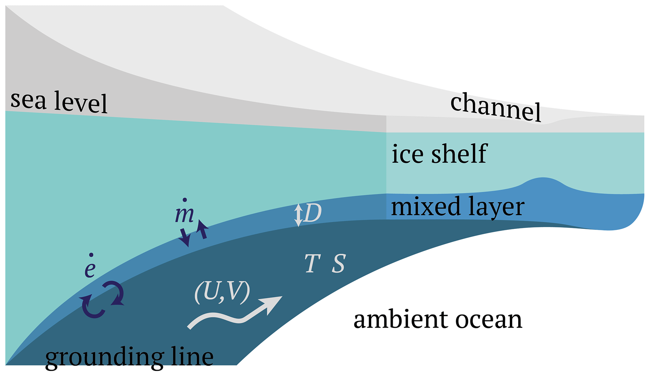
Figure 1 Illustration of the LADDIE model. The model solves for five variables describing the meltwater layer beneath the ice shelf, denoted by the white letters. The dark blue letters denote fluxes at the top of the layer ($\dot{m}$, melt and freezing) and at the bottom of the layer ($\dot{e}$, entrainment and detrainment). The model is forced with geometric boundary conditions (grounding line, ice shelf front and ice shelf topography) and the temperature and salinity of the ambient ocean below the meltwater layer.

The derivation of the pressure gradient terms in these equations is presented for a dense bottom boundary layer by Killworth and Edwards (1999). D is the layer thickness (in m); $\mathit{U}=(U,V)$ is the velocity vector along the ice–ocean interface, containing U and V, the vertically averaged velocities in x and y directions (in m s⁻¹); and T and S are the vertically averaged temperature (in ^∘C) and salinity (in psu). Sources and sinks of layer thickness are both melting and freezing at the ice–ocean boundary, $\dot{m}$, and entrainment and detrainment at the bottom of the meltwater layer, $\dot{e}$. These fluxes are directed into the meltwater layer, and thus $\dot{m}>\mathrm{0}$ denotes net melt and $\dot{e}>\mathrm{0}$ denotes net entrainment. These fluxes are expressed as velocities perpendicular to the model's plane, and their parameterisation is described in Sect. 2.1.2. A_h is the horizontal viscosity, K_h the horizontal diffusivity and γ_T is the turbulent exchange velocity of heat in the ice–ocean boundary layer; the latter is parameterised as described in Sect. 2.1.2. Note that we assume ice to be of salinity 0; hence, no melt term appears in the salt budget.

The subscript a refers to variables in the motionless “ambient” ocean below the layer and to variables at the interface between the layer and the ambient water below; $g_{\mathrm{a}}^{\prime }$ is the reduced gravity, describing the effective gravitational acceleration due to density differences in seawater:

$$\begin{array}{}\text{(6)}& g_{\mathrm{a}}^{\prime }=g{\displaystyle \frac{\mathrm{\Delta }{\mathit{\rho }}_{\mathrm{a}}}{{\mathit{\rho }}_{\mathrm{0}}}}.\end{array}$$

Δρ_a is the density difference between the layer and the ambient water below the layer. We assume a linear equation of state as follows:

$$\begin{array}{}\text{(7)}& \mathrm{\Delta }{\mathit{\rho }}_{\mathrm{a}}={\mathit{\rho }}_{\mathrm{0}}(-\mathit{\alpha }(T_{\mathrm{a}}-T)+\mathit{\beta }(S_{\mathrm{a}}-S\left)\right).\end{array}$$

The ambient temperature T_a and salinity S_a function as forcing fields in the model. These depth-dependent variables are derived from external input, as described in Sect. 2.3.2. In this equation, α is the thermal expansion coefficient, while β is the haline contraction coefficient.

The subscript b refers to the ice shelf base and variables at the ice–ocean interface; z_b is the depth of the ice shelf draft in metres below sea level (depth is defined negative: z_b<0); T_b is the temperature at the ice–ocean boundary.

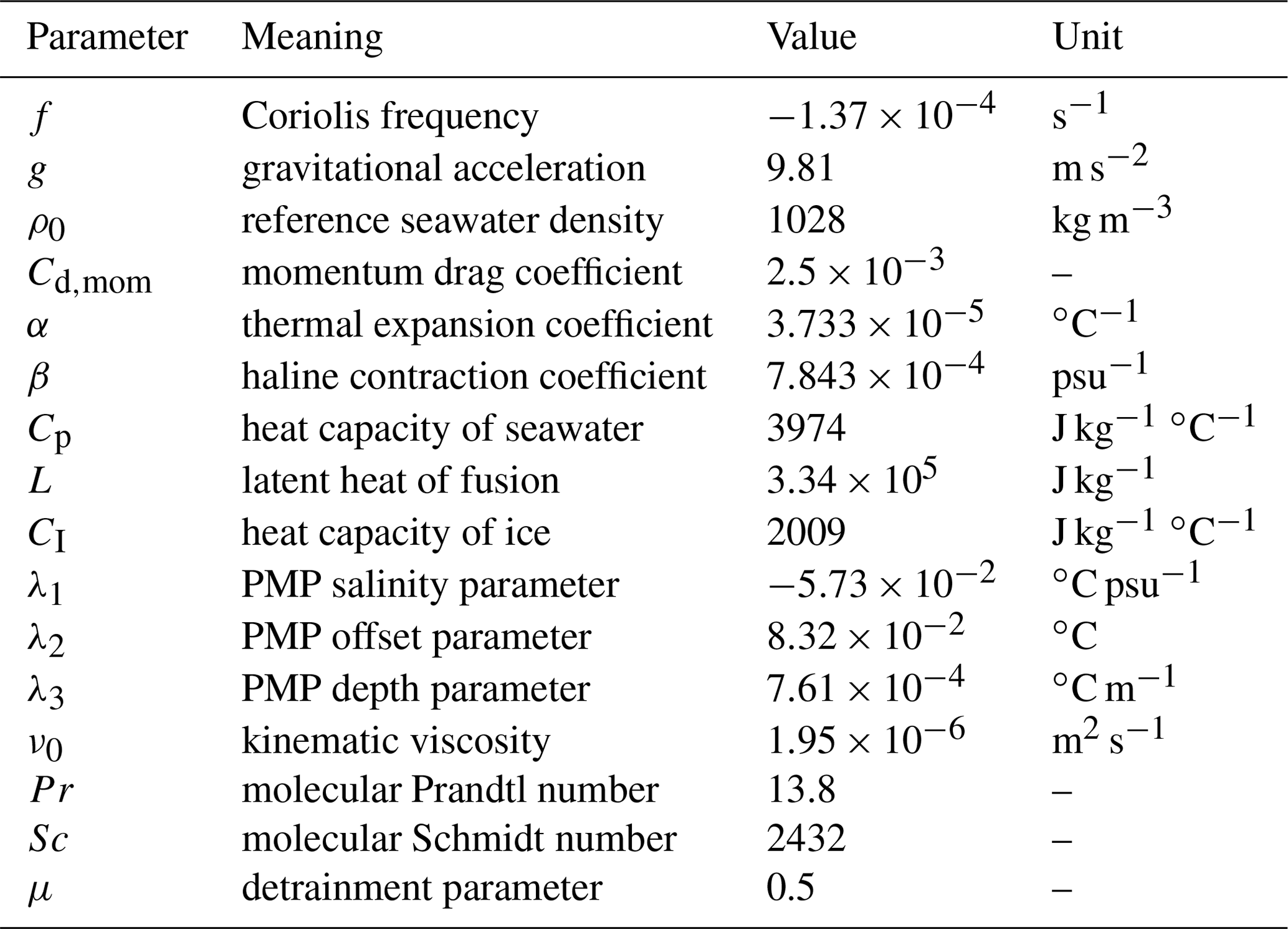
The remaining fixed parameters are the Coriolis frequency f, the gravitational acceleration g, the reference density ρ₀ and the momentum drag coefficient C_d,mom. All fixed parameter values are given in Table 1. Finally, a number of parameters are used as tuning parameters or adapted to assure numerical stability under different configurations. These parameter values are listed in Table 2.

2.1.2 Boundary conditions

The vertical exchange of volume, heat and salt is governed by freezing or melt ($\dot{m}$ at the top boundary) and entrainment or detrainment ($\dot{e}$ at the bottom boundary). Here, we describe LADDIE's parameterisations governing $\dot{m}$ and $\dot{e}$, as well as its lateral boundary conditions.

The top boundary condition $\dot{m}$ is computed by solving the widely adopted “three-equation” formulation for melt and freezing, comprising the conservation of heat and salt, as well as an equation constraining the ice–ocean boundary to remain at the freezing point (Holland and Jenkins, 1999; Jenkins et al., 2010):

$$\begin{array}{}\text{(8)}& {\displaystyle }{C}_{\mathrm{p}}{\mathit{\gamma }}_{\mathrm{T}}(T-T_{\mathrm{b}})=\dot{m}L+\dot{m}{C}_{\mathrm{I}}(T_{\mathrm{b}}-T_{\mathrm{i}}),\text{(9)}& {\displaystyle }{\mathit{\gamma }}_{\mathrm{S}}(S-S_{\mathrm{b}})=\dot{m}{S}_{\mathrm{b}},\text{(10)}& {\displaystyle }{T}_{\mathrm{b}}={\mathit{\lambda }}_{\mathrm{1}}{S}_{\mathrm{b}}+{\mathit{\lambda }}_{\mathrm{2}}+{\mathit{\lambda }}_{\mathrm{3}}{z}_{\mathrm{b}}.\end{array}$$

Here, T_i is the temperature of the ice shelf interior, which functions as a forcing parameter. C_p is the heat capacity of seawater, C_I is the heat capacity of ice, L is the latent heat of fusion for ice, and T_b and S_b are the temperature and salinity at the ice–ocean interface. The three parameters λ_n specify the pressure melting point.

In the above parameterisation for $\dot{m}$, γ_T and γ_S are the turbulent exchange velocities of heat and salt (in m s⁻¹), which we parameterise as follows Jenkins (1991):

$$\begin{array}{}\text{(11)}& {\displaystyle }{\mathit{\gamma }}_{\mathrm{T}}={\displaystyle \frac{U_{*}}{\mathrm{2.12}\log (U_{*}D/{\mathit{\nu }}_{\mathrm{0}})+\mathrm{12.5}P{r}^{\mathrm{2}/\mathrm{3}}-\mathrm{8.68}}},\text{(12)}& {\displaystyle }{\mathit{\gamma }}_{\mathrm{S}}={\displaystyle \frac{U_{*}}{\mathrm{2.12}\log (U_{*}D/{\mathit{\nu }}_{\mathrm{0}})+\mathrm{12.5}S{c}^{\mathrm{2}/\mathrm{3}}-\mathrm{8.68}}}.\end{array}$$

Here, ν₀ is the kinematic viscosity, while Pr and Sc are the molecular Prandtl and Schmidt numbers of seawater, respectively.

In the latter equations, U_* is the friction velocity, defined as in Jenkins et al. (2010) as follows:

$$\begin{array}{}\text{(13)}& U_{*}=\sqrt{C_{\mathrm{d},\mathrm{top}}(U^{\mathrm{2}}+V^{\mathrm{2}}+U_{\mathrm{tide}}^{\mathrm{2}})}.\end{array}$$

Here, U_tide is a time-mean tidal velocity (in m s⁻¹), which functions as a forcing parameter for the model. C_d,top is a drag coefficient applied only to the friction velocity used in the melting formulation (Eq. 8). Note that, following Asay-Davis et al. (2016), we introduce this separate drag coefficient alongside C_d,mom, which is used in the momentum equations (Eqs. 2, 3). This separation into two drag coefficients is sometimes applied in 3D ocean models to correct for neglected processes, such as stratification, in the melting formulation (see discussion by, e.g. Holland and Feltham, 2006). In the current study, C_d,mom is fixed (Table 1), whereas C_d,top is treated as a tuning parameter (Sect. 2.3.3).

The bottom boundary conditions govern the entrainment $\dot{e}$ of ambient water into the meltwater layer. This entrainment has been described by a wide variety of different parameterisations (Jenkins, 1991; Holland and Feltham, 2006). In each of these parameterisations, entrainment is expressed as a function of the turbulent velocity in the meltwater layer. However, under conditions of weak turbulence, detrainment may occur. This process reverses the transport between the upper layer and the ambient waters, thinning the layer. Detrainment is an important process to prevent the layer thickness from growing indefinitely. We therefore follow Gladish et al. (2012) in adopting the parameterisation from Gaspar (1988) describing entrainment and detrainment from an ocean surface mixed layer:

$$\begin{array}{}\text{(14)}& {\displaystyle \frac{D}{\mathrm{2}}}{g}_{\mathrm{b}}^{\prime }\dot{m}+{\displaystyle \frac{D}{\mathrm{2}}}{g}_{\mathrm{a}}^{\prime }\dot{e}=\mathit{\mu }{U}_{*}^{\mathrm{3}}.\end{array}$$

Here, μ is a nondimensional parameter. Negative values for $\dot{e}$ represent detrainment fluxes. This parameterisation describes the balance between the source of turbulent kinetic energy (TKE) from frictional stress at the ice base (U_* term) and the buoyancy sink of TKE from melting and entrainment. In this expression, the dissipation of TKE is assumed to occur as a fixed fraction of the rate of TKE production and is therefore embedded in the parameter μ. This parameterisation was previously used in the 3D ocean model MICOM (Holland and Jenkins, 2001) and in an earlier example of the layer model (Gladish et al., 2012). Note that the same value for U_* is used, based on C_d,top, as in Eq. (8). Whether C_d,mom or C_d,top is the more appropriate choice for Eq. (14) can be debated. However, as μ is an arbitrary constant that can be tuned accordingly, both options are equivalent.

The lateral boundary conditions in LADDIE are split between closed and open boundaries. The closed boundaries apply at the grounding line, where the ice shelf cavity meets the grounded ice. Here, zero gradients are prescribed in D, T and S. In addition, a partial slip condition is prescribed for U and V, similar to that included in the NEMO model (Madec et al., 2019). To optimise the flexibility of the model, this partial slip condition describes a spectrum between free slip and no slip, rather than only allowing the latter two options. In the partial slip condition, lateral friction is scaled down compared to no slip. The slip condition is governed by a parameter ranging between 0 (free slip) and 2 (no slip). In the current study, we apply a value of 1, though a sensitivity analysis revealed that the parameter choice has a weak impact on the simulated basal melt patterns.

At the open boundaries, where the cavity meets the open ocean below the ice-shelf front, zero gradients are applied to all variables, i.e. D, T, S, U and V. These conditions allow the model to converge to a steady solution where the net outflow from the cavity into the deep ocean balances the integrated volume, heat and salt fluxes due to entrainment and melt.

Table 1 Model parameters. PMP stands for pressure melting point.

2.1.3 Numerical implementation

The horizontal grid is discretised as a staggered Arakawa-C grid, in which velocities U and V are solved at the grid cell edges and the other variables D, T and S are solved at grid centres. The advection of volume, heat and salt is applied using an upstream-biased advection scheme. After trial-and-error testing of various options, this scheme was found to be most stable.

The numerical integration in time is performed using a leapfrog scheme with a Robert–Asselin filter, similar to that in the NEMO model (Madec et al., 2019). This filter functions as a diffusion in time and is set by parameter ν between 0 and 1. In the NEMO model description, ν=0.1 is presented as a reference value. Using this same value in LADDIE was found to require a relatively short time step to maintain numerical stability. We found that a value of ν=0.8 produces identical steady-state solutions while allowing for a longer time step. Because in this study we only focus on steady-state solutions, we chose to keep the value of ν=0.8. However, the choice of ν does affect the transient state, and future applications of the model should reassess this parameter choice.

A general issue in 2D models, similar to isopycnal 3D models, is that the model requires a finite thickness D in order to remain numerically stable. In some regions, set by the topography of the ice shelf draft z_b, the velocity field tends to be divergent, particularly near grounding lines. In some cases, the entrainment flux $\dot{e}$ is insufficient to compensate for this divergent flow, leading to a gradual thinning of the model layer. This issue was discussed in detail by Gladish et al. (2012), who proposed the solution of imposing a minimum layer thickness D_min. One can interpret this solution as being equivalent to the fixed upper grid thickness in 3D ocean models. Here, we adopt this solution by increasing the local entrainment flux as required when the thickness would otherwise drop below D_min. We treat the parameter D_min as a tuning parameter, as described in Sect. 2.3.3.

2.2 External data

For the model simulations and evaluation, we use a number of data sets from external sources. Here, we briefly discuss their source, their underlying methodology and some of their limitations.

2.2.1 Geometry

The realistic simulation of ice shelf basal melt rates with LADDIE strongly depends on the applied geometry. Here, we have taken the geometry from the BedMachine v2 data set (Morlighem et al., 2020). This data set combines remote sensing products of the Antarctic ice surface elevation and velocity into a consistent map of ice thickness and bed topography below grounded ice. For the floating ice shelves, the ice shelf thickness is based on the assumption of hydrostatic equilibrium, a modelled firn layer and an additional firn depth correction. Within 3 km from the grounding line, the authors have smoothed the ice shelf thickness to ensure continuity.

While providing a detailed, high-resolution geometry, the BedMachine data set contains some limitations that are relevant to our study. The smoothing within 3 km from the grounding line removes detailed topographic features in this region. In addition, the grounding line is static, which prevents the modelling of basal melt nearby retreating grounding lines. At small scales, the assumption of hydrostatic equilibrium may also be violated by a significant internal stress, obscuring the topography of basal channels. Finally, the data set provides a snapshot of the highly dynamic ice shelf front and shear margins. This allows LADDIE to simulate instantaneous basal melt rates, but these melt rates may not be representative of a multi-year period in some regions.

2.2.2 Observations

To quantitatively evaluate LADDIE, we compare the simulated basal melt patterns to basal melt rates derived from remote sensing products. For simplicity, we refer to these basal melt rates as “observations”, while stressing that they are highly uncertain and based on a range of assumptions. Therefore, these observations should not be interpreted as a ground truth.

For the Crosson–Dotson Ice Shelf, we evaluate LADDIE against observations from Gourmelen et al. (2017) and Goldberg et al. (2019). These basal melt rates are derived from CryoSat-2 radar altimetry over the period 2010–2016. Changes in surface elevation are processed using a Lagrangian analysis based on observed surface ice velocities. Together with modelled surface mass balance and the assumption of hydrostatic equilibrium, these observations are used to construct a mass balance, from which basal melt rates are derived.

Besides uncertainties in the underlying observations, the assumption of hydrostatic equilibrium induces a large uncertainty near grounding lines. This uncertainty was assessed by Milillo et al. (2022) for the Crosson–Dotson Ice Shelf and was found to be small in the Kohler grounding zone but large in the Smith grounding zone. Another issue with observations in the grounding zone is the timing and the relatively long period over which basal melt rates are assessed. The Kohler, Smith and Pope grounding lines are known to have retreated at a high rate over the last decade (Scheuchl et al., 2016; Milillo et al., 2022). This makes average basal melt rates over a multi-year period in this region (e.g. Gourmelen et al., 2017) less representative of instantaneous basal melt rates as simulated by LADDIE.

For the Filchner–Ronne Ice Shelf, we use the Antarctic-wide observations from Adusumilli et al. (2020). The underlying methodology is similar to that of Gourmelen et al. (2017); it is based on a combination of CryoSat-2 altimetry, satellite-derived surface ice velocities, and modelled firn layer. The firn density model used in this study is of a coarse resolution (12.5 km) compared to the grid size of the final product (500 m). In addition, no recalibration based on local observations is applied as in Gourmelen et al. (2017). Together, these differences lead to a poorer spatial detail in the “observed” basal melt fields. However, comparison to other remote sensing estimates (Rignot et al., 2013; Moholdt et al., 2014) gives confidence to the assessed large-scale pattern of basal melting and freezing.

2.2.3 The 3D model reference

In this study, we introduce LADDIE as a new model to simulate high-resolution spatial basal melt patterns. To test its added value compared to 3D numerical ocean models, we compare the simulated basal melt fields for Crosson–Dotson and Filchner–Ronne to regional 3D model output. This comparison output is chosen for the quality of the basal melt patterns, its availability and its representation of a steady state.

For the Crosson–Dotson Ice Shelf, we compare basal melt from LADDIE to that simulated by a regional setup of MITgcm of the Amundsen region with resolved ice shelf cavities (Naughten et al., 2022). The ocean and sea ice model is configured with a horizontal grid size ranging from 5.2 km offshore to 2.8 km at its southernmost point. The geometry is based on the BedMachine v2 geometry and the model is forced with ERA5 atmospheric reanalysis (Hersbach et al., 2020). The model was extensively tuned to reproduce observations in the region. In particular, the ocean conditions and their interannual variability in front of Dotson and Pine Island ice shelves were tuned to match observations by varying sea ice parameters, and then the melt rates for these ice shelves were tuned to match observations by selecting melting parameter values that best fit the entire region (Naughten et al., 2022). For an optimal comparison to the observations from Rignot et al. (2013), we extract and average the period 2003–2008 from the MITgcm simulation.

For the Filchner–Ronne Ice Shelf, we compare the basal melt rates from LADDIE to regional simulations using NEMO (Hausmann et al., 2020). NEMO, similar to MITgcm, is an advanced ocean and sea ice model with explicitly resolved cavities. The regional simulation of the Weddell Sea was configured at a horizontal resolution varying between 4.5 km offshore to 1.5 km at the southernmost point. The model was forced with atmospheric climatology from CORE-2 (Large and Yeager, 2009) and tidal conditions at the open boundaries from FES2012 (Carrere et al., 2013). The model was specifically designed to simulate tides in the Filchner–Ronne cavity and their impact on basal melt and freezing.

Both 3D ocean and sea ice models are configured using a fixed vertical grid. The vertical grid cell thickness below the ice shelves ranges between 10 and 50 m for MITgcm and between 10 and 150 m for NEMO. In both models, basal melt and freezing is parameterised using a similar “three-equation” formulation to that used in LADDIE (Eq. 8).

2.3 Model setup

In this section, we describe the model setup for the simulations of the Crosson–Dotson and Filchner–Ronne Ice shelves (Fig. 2).

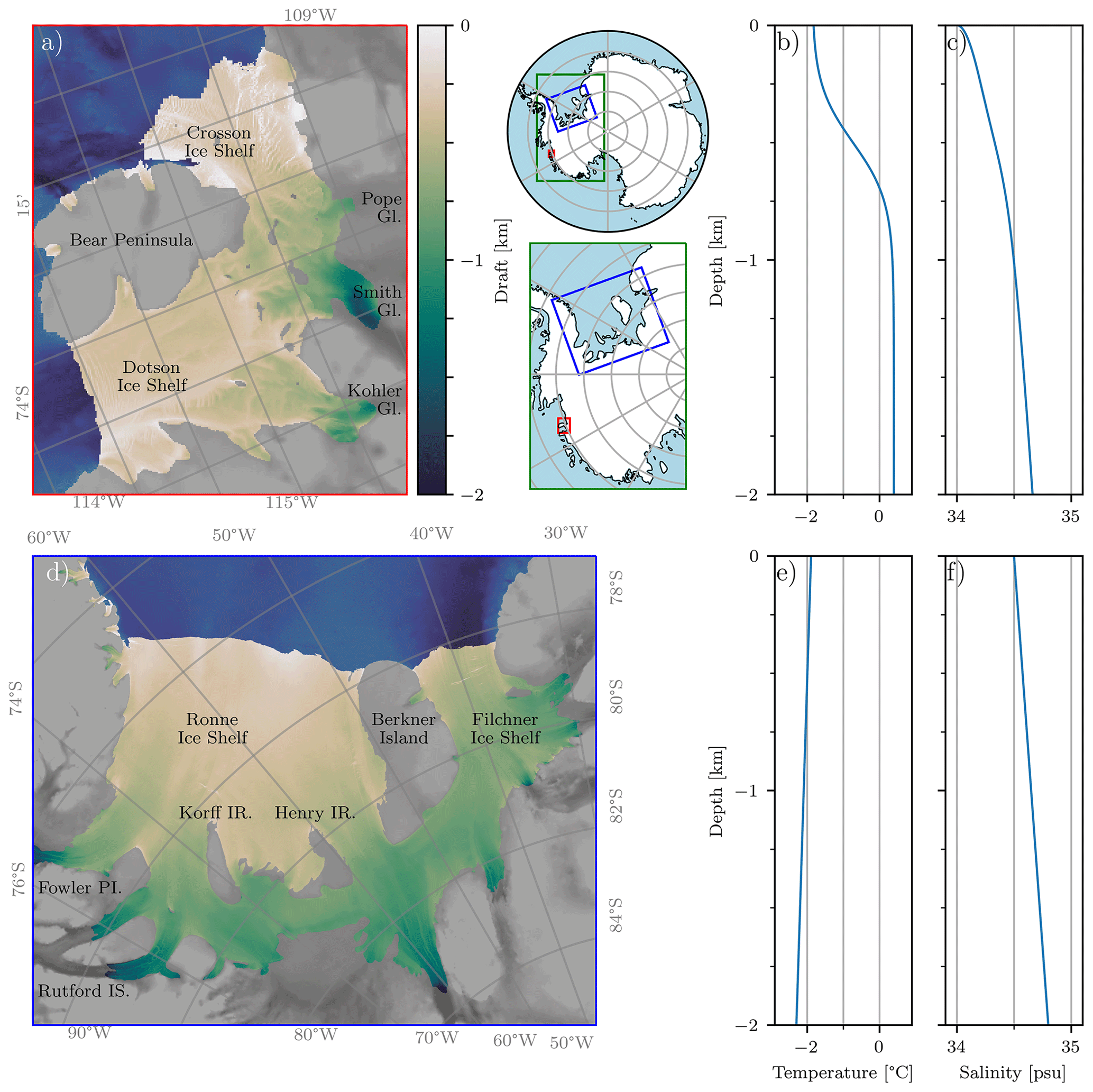
Figure 2 Geometry and forcing for the Crosson–Dotson and Filchner–Ronne ice shelves. (a, d) Ice shelf geometries. The bright shading indicates the ice shelf draft, increasing from the grounding line to the ice shelf front. The low-contrast shading denotes the bed topography below the open ocean (dark blue) and the grounded ice sheet (grey), with dark colours indicating a deep bed. The locations are indicated with the inset overview maps between (a) and (b). Abbreviations are as follows: “Gl.” is glacier, “IS.” is ice stream, “IR.” is ice rise, and “PI.” is peninsula. (b, c, e, f) Idealised vertical temperature and salinity forcing profiles applied in the main simulations.

2.3.1 Geometry

Due to its relatively small size, the Crosson–Dotson Ice Shelf can be configured on the original resolution of 500×500 m² of the BedMachine v2 data set (Morlighem et al., 2020) without a problem. Note that previous studies have smoothed the ice shelf topography, in part to ensure numerical stability (e.g. Holland et al., 2007), which is a common practice in ice–ocean modelling (e.g. Asay-Davis et al., 2016). In order to resolve kilometre-scale basal melt features, LADDIE is configured such that it can deal with unmodified ice shelf topography.

For the Filchner–Ronne Ice Shelf, simulations at 500×500 m² are computationally demanding, as the LADDIE model is not yet coded in parallel. Hence, this ice shelf is configured at a 1000×1000 m² resolution by averaging the topography of 2×2 neighbouring grid cells.

2.3.2 Forcing

The LADDIE model takes four variables as external forcing: the ambient temperature and salinity, T_a and S_a; the ice shelf temperature T_i; and the tidal velocity U_tide. In this study, we apply idealised forcing fields, allowing for a straightforward interpretation of the results and a clean assessment of the geometric impact on basal melt patterns. To test the sensitivity of the basal melt patterns to this choice of idealised forcing, we include a comparison for Crosson–Dotson to a more realistic 3D forcing (Appendix A).

For both the Crosson–Dotson and Filchner–Ronne ice shelves, we apply uniform fields of T_i and U_tide. The values are listed in Table 2. We note that U_tide has a large impact on the heat transfer toward the ice shelf base. In particular for Filchner–Ronne, an accurate spatially heterogeneous tidal forcing may significantly improve the accuracy of basal melt patterns (Hausmann et al., 2020). However, we note that the tidal fields used most commonly to force 3D ocean models contain substantial errors in several Filchner–Ronne grounding zones (Padman et al., 2018). As we discuss in Sect. 3.2.2, this can lead to erroneous basal melt patterns. A detailed assessment of the accuracy and impact of tidal forcing is beyond the scope of this study, and we therefore proceed with uniform tidal forcing.

For T_a and S_a, the main results in this paper are based on idealised vertical profiles of temperature and salinity. We choose this approach for a number of reasons. First, as described above, an idealised forcing eases the interpretation of the geometric impact on the simulated basal melt patterns. Second, 1D vertical profiles resemble the output of Earth system models without resolved cavities; we anticipate that forcing with such ESM output will be a main application of the model. Third, observations in front of the ice shelves are available (Nicholls et al., 2009; Jenkins et al., 2018), yet these are subject to a summer bias and substantial interannual variability; whether these observations are representative of the long-term ocean state is unclear. Based on this reasoning, we choose to present model results based on simulations with idealised 1D forcing.

The forcing profiles for both ice shelves are shown in Fig. 2. The profiles for Crosson–Dotson mimic an average state from the observations by Jenkins et al. (2018). Temperature is described by a tangent hyperbolic function, ranging from −1.7 ^∘C at the surface to +0.4 ^∘C at 1200 m depth (Fig. 2b). The thermocline is centred at 500 m depth with a scale factor of 250 m. This temperature profile describes the observed two-layer stratification in front of the ice shelf. Salinity increases from 34 psu at the surface to 34.5 psu at 1200 m depth. The profile is derived from a prescribed density profile, which is quadratic with depth; this density profile mimics the observed stratification maximum near the surface.

For the Filchner–Ronne Ice Shelf, we apply idealised profiles of temperature and salinity approximating the average conditions within this cold cavity. These profiles are similar to those applied to the Filchner–Ronne simulations by Holland et al. (2007). Temperature decreases linearly from freezing point at the surface to −2.3 ^∘C at 2000 m depth. Salinity increases linearly from 34.5 psu at the surface to 34.8 psu at 2000 m depth (Fig. 2f).

From these vertical profiles, at each model time step, temperatures and salinities at each grid cell are extracted at the depth of the layer base, z_b−D. These temperatures and salinities form the horizontal 2D fields of T_a and S_a at the layer base.

In Appendix A, we present an additional use case for Crosson–Dotson. Here, the model is forced with 3D cavity fields from simulations with MITgcm (see Sect. 2.2.3). We describe this more advanced forcing and its impact on basal melt patterns in Appendix A. In addition, this 3D forcing is used to tune the model, as described in detail in Appendix B.

2.3.3 Parameter settings

With the geometry and forcing described above, the model setup is completed by a number of parameter choices. A number of parameter values remain unspecified in order to adapt them to different simulations. These are the time step Δt, the horizontal viscosity A_h and the horizontal diffusivity K_h; each of these affects the numerical stability of the model and depend on the chosen resolution. Finally, two parameters are considered tuning parameters: C_d,top and D_min.

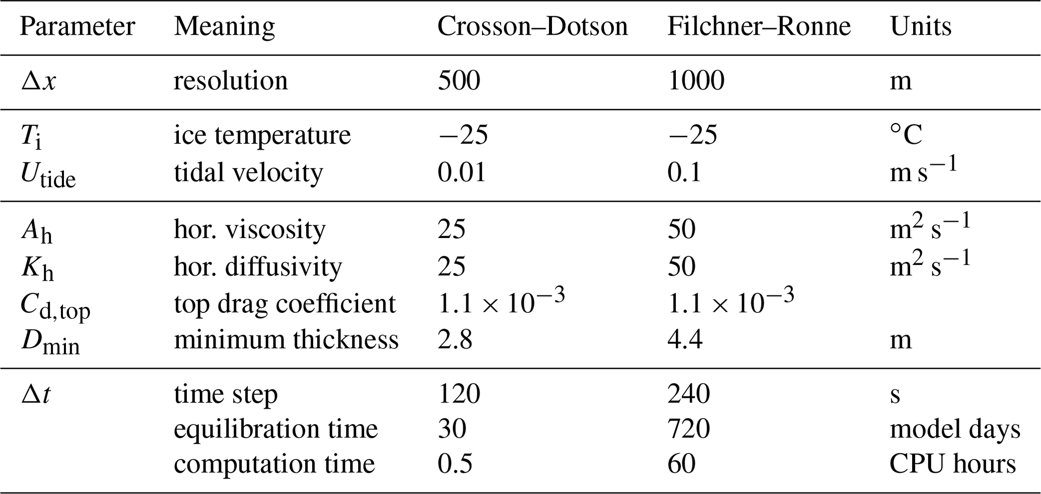
Based on trial and error, we have determined values of A_h of 100, 50 and 25 m² s⁻¹ to be suitable for grid resolutions of 2000, 1000 and 500 m, respectively. Further sensitivity runs indicated that the choice of K_h has only a small effect on the resultant basal melt rates; for convenience, we take K_h equal to A_h. Finally, values for the time step Δt are determined per configuration in order to maximise the time step while ensuring numerical stability. The values for the main simulations of the Crosson–Dotson and Filchner–Ronne ice shelves are shown in Table 2. Note that the values of A_h and K_h exceed those of Asay-Davis et al. (2016) for reasons of numerical stability; lower values can be used when sufficiently reducing the time step Δt and/or smoothing the topography.

We have chosen to treat the remaining two parameters as tuning parameters, namely the drag coefficient used in the equation for the friction velocity C_d,top and the minimum layer thickness D_min. C_d,top is commonly used for tuning the basal melt parameterisation in ocean models (Holland and Feltham, 2006); values in the literature vary between $\mathrm{1.0}\times {\mathrm{10}}^{-\mathrm{3}}$ (Jourdain et al., 2017; Mathiot et al., 2017) and $\mathrm{9.7}\times {\mathrm{10}}^{-\mathrm{3}}$ (Jenkins et al., 2010). D_min is treated as a tuning parameter, as its impact on basal melt rates is found to be relatively large. Here, we have considered values between 2 and 8 m.

The model is tuned to a number of observation-based indicators for the Crosson–Dotson Ice Shelf. The resultant tuning parameters are applied to the Filchner–Ronne Ice Shelf in order to test whether the tuning is valid in both cold and warm environments. Five diagnostics are derived from simulations with 3D forcing: ice-shelf-average melt, melt in the Kohler grounding zone, melt along the wide Dotson Channel and along its centre line, and the total overturning circulation. These diagnostics are compared to a number of remote sensing and in situ observational sources. For horizontal grid sizes of 500×500, 1000×1000 and 2000×2000 m², values of D_min and C_d,top are determined such that each of the five diagnostics falls within the assessed uncertainty ranges. The complete tuning procedure is described in Appendix B, and the values used in our simulations are shown in Table 2.

We note that the model is tuned to Crosson–Dotson and partly evaluated on the same ice shelf. However, only two tuning parameters are used for five tuning targets and an evaluation of the complete melt pattern. Therefore, we consider this tuning procedure to be valid. As additional proof of the validity of this tuning procedure, we include a simulation for the Pine Island Ice Shelf, another small ice shelf in the warm Amundsen Sea region, in Appendix C.

Table 2 Simulation-specific parameter values applied the Crosson–Dotson and the Filchner–Ronne ice shelves.

2.3.4 Experimental design

Using the configuration and parameter settings above, the equations are integrated forward in time. The layer is initialised at rest, $U=V=\mathrm{0}$, and the initial layer is uniformly 10 m thick. For temperature and salinity, T and S, initial values are taken 0.1 ^∘C and 0.1 psu below the ambient values T_a and S_a, respectively. This small initial difference in salinity ensures a stable stratification.

The current model setup is designed to simulate basal melt rates under steady-state conditions, with a fixed geometry and fixed ambient conditions. The results presented in this study are thus steady-state basal melt rates. For the Crosson–Dotson Ice Shelf, basal melt rates are averaged over the last 5 model days; for Filchner–Ronne this is done over the last 10 model days. The equilibration time, as well as the computation time required for a full spin-up, is listed in Table 2.

3 Results

In this section, we present the steady-state basal melt patterns simulated by LADDIE for the Crosson–Dotson and the Filchner–Ronne ice shelves consecutively. For each ice shelf, we divide the results into three parts. The first is a model evaluation compared to available observations (Sect. 2.2.2). The second is a comparison to 3D ocean model simulations (Sect. 2.2.3). The third and final part is a description and assessment of novel melt patterns that are simulated by LADDIE but not visible in either the observations or the relatively coarse 3D ocean models.

3.1 Crosson–Dotson

In this section, we describe spatial melt patterns of the Crosson–Dotson Ice Shelf (Fig. 3).

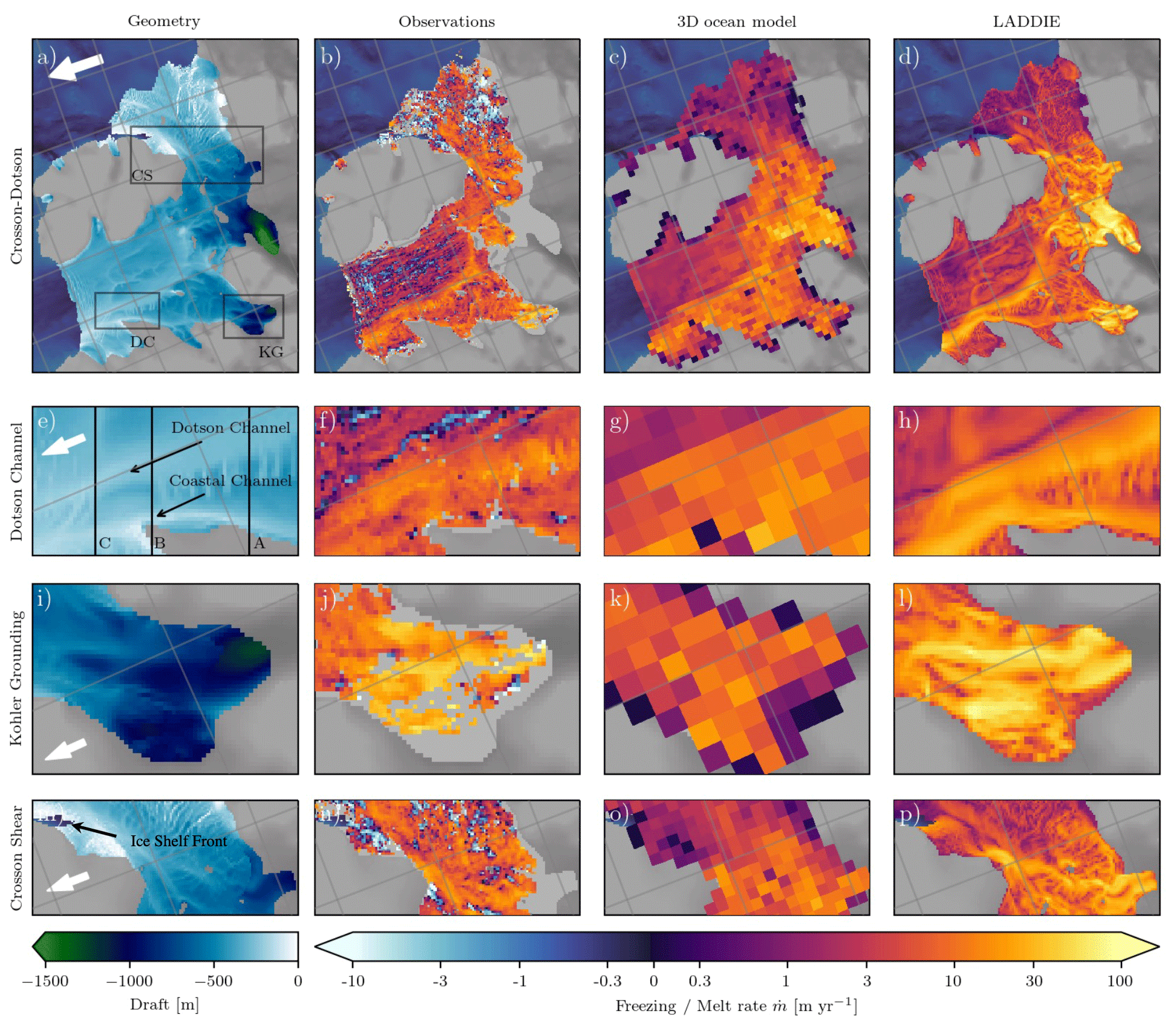
Figure 3 Spatial basal melt field of the Crosson–Dotson Ice Shelf. (a) Geometry in terms of ice shelf draft z_b. Details of the insets are shown in subsequent rows, where DC is the Dotson Channel (shown in e–h), KG the Kohler grounding zone (i–l) and CS the Crosson shear margin (m–p). Place names are labelled in Fig. 2a, and the white arrows point north. The sections indicated in (e) are shown in Fig. 4. (b) Observed basal melt rates from altimetry over the period 2010–2016 (Gourmelen et al., 2017; Goldberg et al., 2020). (c) Basal melt rates from the 3D model MITgcm. (d) Simulated basal melt rates using LADDIE with the vertical forcing profile shown in Fig. 2b–c. The melt colour scale is a symmetrical log scale and is linear between values of −0.3 and 0.3 m yr⁻¹.

3.1.1 Model evaluation

Across the Crosson–Dotson Ice Shelf, remote sensing observations reveal a contrast between high melt rates in deep regions and low melt rates in shallow regions (Fig. 3b). The high melt rates are largely confined to the region where the ice shelf extends below approximately 500 m depth. This depth marks the depth of the thermocline (see Fig. 2c), below which the ice shelf is in direct contact with Circumpolar Deep Water (Jenkins et al., 2018). This relatively warm water mass induces a large temperature difference between the ocean water and the freezing point at the ice shelf base; this temperature difference is defined as the thermal forcing. To the first order, it is this strong thermal forcing that explains the high melt rates in the deep ice shelf regions (e.g. Favier et al., 2019).

In the regions of the ice shelf shallower than the thermocline, a weak thermal forcing induces relatively low basal melt rates (Fig. 3b). The remote sensing observations even indicate basal freezing in some shallow regions; however, this is an artefact of the calculation procedure and is considered unrealistic by Goldberg et al. (2019). Overall, the contrast between high melt in the deeper regions and low melt in the shallow regions is well simulated by LADDIE (Fig. 3d).

This large-scale contrast between the deep and shallow regions is violated by one major feature, the Dotson Channel (DC). While this channel resides in the shallow region of the ice shelf, it contains relatively high melt rates. The Dotson Channel is approximately 5 km wide, is clearly visible in the ice shelf topography (Fig. 3a) and extends from the deep parts of the ice shelf to the shallow ice shelf front (Gourmelen et al., 2017). Channels like the Dotson Channel arise due to meltwater plumes that advect relatively warm water from the deep ice shelf regions to the shallow regions (Payne et al., 2007). The accurate modelling of such melt channels therefore requires the explicit simulation of the flow below the ice shelf. As a consequence, melt channels cannot easily be simulated using models of fewer than two dimensions (e.g. Burgard et al., 2022). The regional melt enhancement in the DC, 1.2 times the ice shelf–average basal melt rate, was part of the tuning procedure in this study (Appendix B). We found that this melt enhancement is relatively insensitive to variations in the tuning parameters. Hence, we conclude that the Dotson Channel is robustly and realistically simulated by LADDIE.

The evaluation of the LADDIE model is continued by a closer look at the detailed melt pattern across the Dotson Channel. An enlargement of part of the Dotson Channel is shown in Fig. 3e–h. One remarkable feature revealed by the remote sensing observations is the misalignment between the centreline of the topographic channel (Fig. 3e) and the centreline of the observed melt peak (Fig. 3f). This misalignment is visualised more clearly in three cross sections across the Dotson Channel in Fig. 4. Across all three sections, the observed melt peak (orange curves) aligns to the left (west) of the channel's topographic centreline (vertical black lines). This westward amplification of melt rates occurs due to the Coriolis deflection of the northward-flowing melt plume, which is directed toward the left in the Southern Hemisphere. These remote sensing observations of Coriolis-enhanced melt by Gourmelen et al. (2017) are supported by observations of basal melt of the Pine Island Ice Shelf (Dutrieux et al., 2013). The asymmetry in melt rates within the Dotson Channel favours a channel geometry that is directed to the left of the ice shelf flow direction (Dutrieux et al., 2013) and can potentially induce a westward migration of the channel due to ice–ocean interactions (Gladish et al., 2012; Sergienko, 2013). The observed misalignment between the topographic channel and the melt peak is accurately reproduced by LADDIE (light-blue curves). This agreement indicates that both the flow of the melt plume and the Coriolis deflection thereof are realistically simulated by LADDIE.

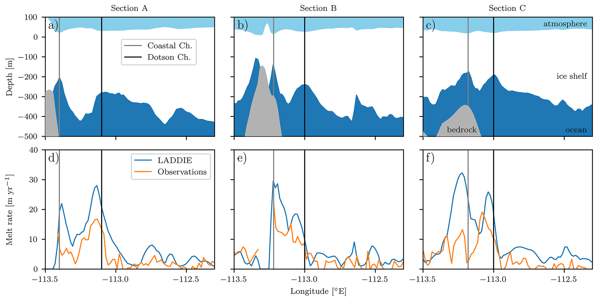
Figure 4 Cross sections across the Dotson and Coastal channels. The location of sections A, B and C are indicated in Fig. 3e. (a–c) Geometry including the ice shelf (white), ocean cavity (blue) and solid earth (grey). The vertical lines indicate the topographic locations of the channel centrelines. (d–f) Observed and simulated basal melt rates across the same sections.

As a final region to evaluate the LADDIE performance of the Crosson–Dotson melt pattern, we look more closely at the Kohler grounding zone (Fig. 3i–l). This is the only deep grounding zone of this ice shelf where valid observations from remote sensing are available. The average melt rates in the grounding zone, derived from remote sensing, are approximately 25 m yr⁻¹ (Fig. 3j; Gourmelen et al., 2017). These rates agree well with the average melt rates of 20 m yr⁻¹ from airborne surveys over the same period (Khazendar et al., 2016). These melt rates are approximately 3–4 times higher than the average melt rates over the whole Crosson–Dotson Ice Shelf over the same period (Gourmelen et al., 2017). We found that this regional melt enhancement can be reproduced by LADDIE depending on the tuning. Whether the melt enhancement in the Kohler grounding zone is realistically simulated thus depends primarily on the model resolution and the choice of D_min.

3.1.2 Inter-model comparison

In some regions of the Crosson–Dotson ice shelf, observations are either absent or inconclusive. In these regions, it is worthwhile to compare the simulated melt rates of LADDIE to output from the 3D ocean model MITgcm. The primary regions where observations are absent are the grounding zones of the Smith and Pope glaciers. In these grounding zones, both models simulate enhanced melt rates comparable to those in the Kohler grounding zone. The simulated melt in these grounding zones mainly differs between the two models at small-scale detail; this difference arises from the higher spatial resolution of LADDIE.

In the shallow regions, the observations are inconclusive with regard to melt or refreezing. In these regions, both models produce weak positive basal melt rates, supporting the assessment that the observed refreezing rates are unrealistic. Overall, the large-scale melt patterns of LADDIE and MITgcm are similar and consistent, providing confidence that the simulated physics is consistent as well.

Another region where remote sensing products do not provide reliable estimates for basal melt is at the grounding line. Remote sensing observations rely on the assumption of flotation, an assumption that fails near the grounding line. However, in situ observations are available from the neighbouring Thwaites grounding line (Davis et al., 2023). These observations revealed low melt rates in grounding line regions with a relatively flat ice shelf base. Both MITgcm and LADDIE reproduce these low melt rates at flat grounding line regions. A major difference between the models arises at specific grounding line regions with a steep topography. MITgcm simulates near-zero melt rates along the complete grounding line, whereas LADDIE simulates high melt rates at these locations of steep topography. The low melt rates of MITgcm may be caused by the coarse vertical resolution or by a limited barotropic flow along the grounding line. The comparably high grounding line melt rates in LADDIE are strongly influenced by the model parameter D_min. Whether the localised high melt rates simulated by LADDIE are realistic cannot be asserted from presently available observations. Hence, the grounding line is a region where the models, at least in their current setup, are inherently inconsistent.

The last region where we compare LADDIE to MITgcm is the Crosson shear margin (Fig. 3m–p). Ice shelf shear margins are often strongly damaged. This damage breaks the assumption of continuity, a central assumption in the computation of basal melt rates from altimetry; in these damaged shear margins, therefore, remote sensing observations are unreliable. Both MITgcm and LADDIE simulate enhanced melt rates along the coastline of Bear Peninsula. A marked difference between melt patterns from LADDIE and MITgcm appears near the ice shelf front. LADDIE simulates relatively high melt rates in the region where the melt plume exits the ice shelf cavity. In contrast, MITgcm simulates low melt rates and does not show a trace of a melt plume here. Melt plumes near ice shelf fronts have been identified indirectly by the presence of polynyas (Alley et al., 2016). Such polynyas are observed throughout the Amundsen Sea region, including the Crosson shear margin. This proxy thus provides evidence that the LADDIE melt pattern in the Crosson shear margin is qualitatively realistic. As shear margins are crucial for ice shelf stability (Sun et al., 2017; Lhermitte et al., 2020), the inconsistency between the melt patterns between MITgcm and LADDIE could be significant in the field of ice shelf modelling.

3.1.3 New features

The high-resolution simulations with LADDIE reveal a variety of small-scale melt patterns that cannot be confirmed by either observations or inter-model comparison. Here, we describe these new melt features and assess the potential underlying physics.

The high spatial resolution of LADDIE allows it to simulate the channelisation of melt plumes in a number of regions. One example is the Kohler grounding zone. Through the middle of this grounding zone, LADDIE simulates several elongated melt features. Similar to the Dotson Channel, these channels are carved out in the basal topography of the ice shelf (Fig. 3i). The presence of such channels in both Kohler and Smith grounding zones is supported by the high spatial variability in basal melt rates from radar observations (Khazendar et al., 2016). The melt channels appear not to be connected to the grounding line itself but to originate downstream of the grounding line. Although this disconnection may very well be an artefact of the smoothing applied to the topography (Sect. 2.2.1), it agrees with the assessment by Alley et al. (2016) that melt channels in this warm region are predominantly ocean-sourced channels. Such ocean-sourced channels require a locally enhanced basal melt to originate and persist. We see that LADDIE simulates enhanced basal melt in these channels, indicating that the modelled basal melt patterns can support ocean-sourced basal channels.

Another new feature we observe is located to the west of the Dotson Channel. Along the coastline, high melt rates reveal the presence of another narrow channel; we will call this the Coastal Channel (Fig. 3h). This channel originates in the Kohler grounding zone and merges with the Dotson Channel before it reaches the ice shelf front. The Coastal Channel is clearly visible in the geometry, in both the plan view (Fig. 3e) and the cross sections (Fig. 4). Although the geometry is uncertain near the grounding line, the existence of this Coastal Channel can be explained physically. It is likely that meltwater from the Kohler grounding zone is transported to the ice shelf front in the form of a melt plume. This melt plume would be forced towards the western coastline by Coriolis deflection, forming a boundary current. The enhanced melt rates would deepen the topographic channel, keeping the melt plume in place. In addition, this coastal region is a shear margin, in which ice divergence can facilitate the formation of melt channels (Alley et al., 2019). We thus consider the Coastal Channel (and the enhanced melt within it) to be a realistic feature.

The Dotson and Coastal channels function as conduits for meltwater produced in the deep grounding zones. Looking back at the ice-shelf-wide melt patterns simulated by LADDIE (Fig. 3d), we can distinguish two meltwater pathways. The Dotson Channel appears to provide a pathway for meltwater from the Smith grounding zone. Similarly, the Coastal Channel appears to act as the main pathway for meltwater from the Kohler grounding zone. Near the ice shelf front, these meltwater plumes converge before exiting the ice shelf cavity. Although these two pathways are clearly carved in the ice shelf topography (Fig. 3a), the remote sensing estimates of basal melt (Fig. 3b) do not provide conclusive evidence for their existence.

Besides the two meltwater pathways exiting the Dotson ice shelf front, the melt patterns simulated by LADDIE reveal a third meltwater pathway. A clear melt channel connects the Pope grounding zone to the Crosson Ice Shelf front. Like most melt plumes, this melt plume is channelised by the shape of the basal ice shelf topography. The apparently strict separation of the three pathways may have implications for meltwater forcing of the deep ocean.

3.2 Filchner–Ronne

The second ice shelf we use as a test case for LADDIE is the Filchner–Ronne Ice Shelf. For this ice shelf, we take the same values for the tuning parameters as for Crosson–Dotson, but we adapt the forcing to the generic Weddell Sea climate (see Sect. 2.3.2). The structure of this section is the same as for Crosson–Dotson: we first evaluate the model by comparison to observations, then perform an inter-model comparison to a 3D model and finally discuss several new melt features.

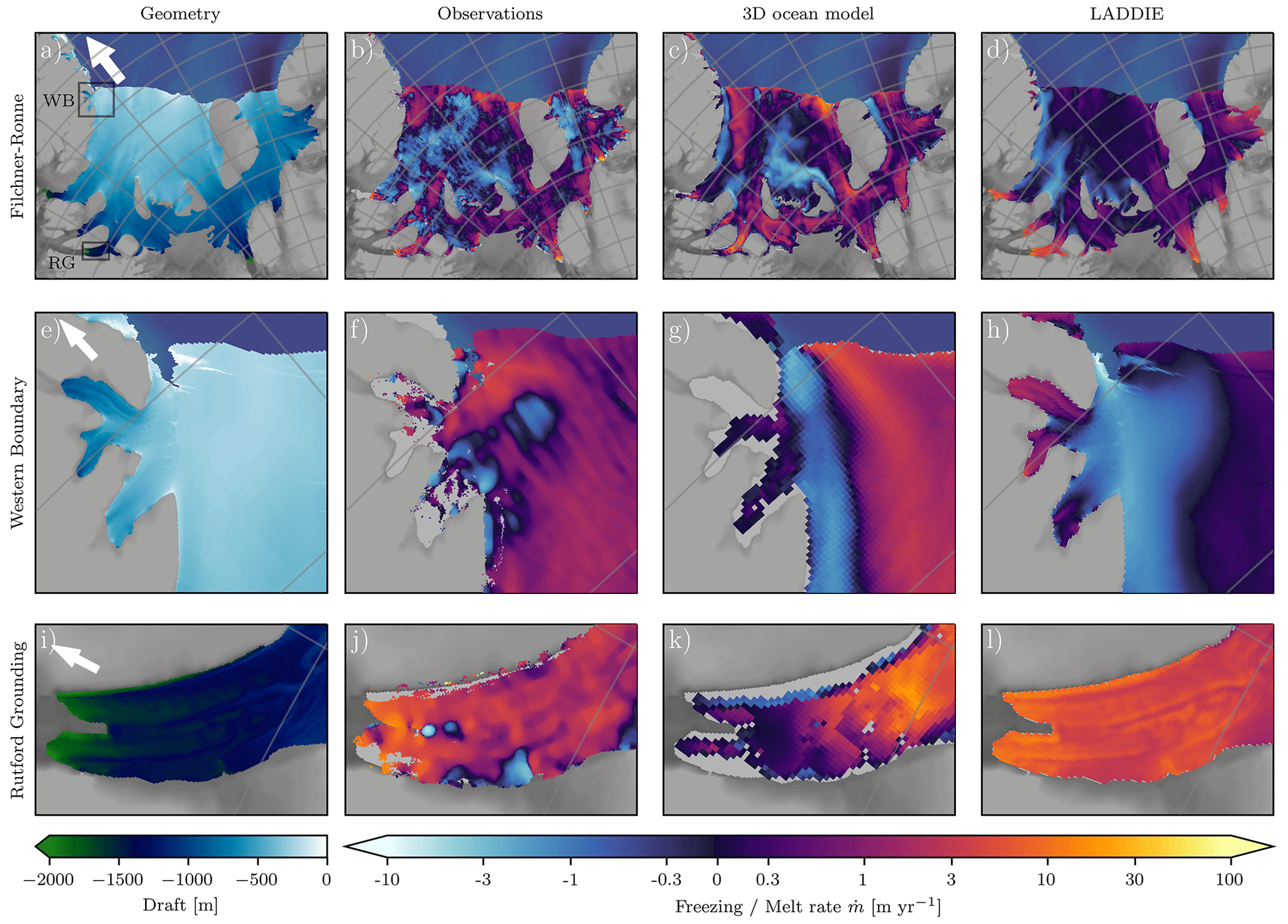
Figure 5 Spatial basal melt field of the Filchner–Ronne Ice Shelf. (a) Geometry in terms of ice shelf draft. Insets shown in subsequent rows refer to the western boundary (WB, shown in e–h) and the Rutford grounding zone (RG, shown in i–l). The white arrows point north. (b) Observed basal melt rates from altimetry Adusumilli et al. (2020). (c) Basal melt rates from the 3D model NEMO including tides (Hausmann et al., 2020). (d) Simulated basal melt rates using LADDIE with the vertical forcing profile in Fig. 2e–f.

3.2.1 Model evaluation

The basal melt rates of the Filchner–Ronne Ice Shelf are considerably lower than those of the Crosson–Dotson Ice Shelf. Observations indicate a spatial average melt rate of 0.32±0.1 m yr⁻¹ (Rignot et al., 2013). This average melt rate is well reproduced by LADDIE (0.26 m yr⁻¹). This agreement implies that LADDIE may be applied to a wide range of ice shelves using a single set of tuning parameters. This reveals an advantage of LADDIE compared to simple basal melt parameterisations, which often require retuning of the melt sensitivity when applied to different ice shelf regions (e.g. Reese et al., 2018a; Jourdain et al., 2020; Burgard et al., 2022; van der Linden et al., 2023). Besides making the model easier to use, this finding provides some confidence that, in terms of the overall melt sensitivity, the dominant physical mechanisms are represented by LADDIE.

Similar to Crosson–Dotson, the highest basal melt rates of Filchner–Ronne are found in the deep grounding zones (Fig. 5b). In contrast to Crosson–Dotson, however, these grounding zone melt rates are not driven by the presence of warm Circumpolar Deep Water. The Filchner–Ronne Ice Shelf cavity is isolated from intrusions of this warm water mass. Instead, this cavity is forced by waters at the surface freezing point formed by sea ice formation offshore (Nicholls et al., 2009); it is therefore classified as a cold cavity. Rather than warm cavity waters, the high melt rates in the grounding zone are caused by the low freezing point at depth. This freezing point, which can reach values of −2.5 ^∘C, is substantially lower than the surface freezing point of approximately −1.9 ^∘C. The ambient waters within the Filchner–Ronne cavity consist of a mixture of water at surface freezing temperature and colder meltwater released at depth. This mixture is warmer than the local freezing temperature within the deep grounding zones, leading to positive melt rates. These show a maximum in the deepest grounding zones where the pressure freezing point reaches a minimum.

The magnitude of the basal melt rates in the grounding zones of Filchner–Ronne is subject to discussion; this complicates the quantitative evaluation of these regional melt rates simulated by LADDIE. Remote sensing estimates, like those in the Rutford grounding zone (Fig. 5i–l), are on the order of 5 m yr⁻¹. The simulated melt rates by LADDIE are of a comparable magnitude. However, in situ observations in the Rutford grounding zone estimate substantially lower basal melt rates of approx. 1 m yr⁻¹ (Jenkins et al., 2006). Further observational research should focus on reconciling these lines of evidence before LADDIE can be evaluated more robustly in this region. It is, however, noteworthy to mention that grounding zone melt rates in LADDIE are closely tied to the tuning parameter D_min. Lower values of grounding zone melt from in situ observations can thus be approached by reducing this tuning parameter.

As the cold meltwater produced in the deepest grounding zones rises toward the ice shelf front, the local freezing point increases. At a certain depth, this meltwater, mixed with ambient water due to entrainment, becomes colder than the local freezing point. This reversed temperature difference sets up a negative thermal forcing, inducing freezing at the ice shelf base. This process, with melt in the deep grounding zone and freezing at intermediate depths, is called the ice pump effect. The remote sensing observations reveal widespread basal freezing across the central ice shelf (Fig. 5b), a finding that is supported by observations of marine ice (Sandhäger et al., 2004; Holland et al., 2007). Qualitatively, LADDIE reproduces basal freezing in the central ice shelf, north of Fowler Peninsula, and along the western boundaries of both the Filchner and Ronne ice shelves (Fig. 5d). These results indicate that the flow direction and cooling of the meltwater plumes originating in the deep grounding zones are well simulated.

Quantitatively, however, a number of discrepancies emerge between LADDIE and observations in the central ice shelf. North of the ice rises, basal refreezing is underestimated, whereas basal melting is underestimated at the southern point of Berkner Island. Both freezing and melt patterns in these regions have been shown to be enhanced by tidal forcing (Hausmann et al., 2020). Hence, the biases in the LADDIE simulations may be reduced by forcing the model with a spatially heterogeneous tidal forcing. In addition, the freezing and melt patterns in these central regions are likely influenced by the barotropic circulation of water masses (e.g. Naughten et al., 2021). The underestimation of spatial variability in basal melt and freezing by LADDIE may thus partly be caused by the assumption of a stationary ambient ocean, as discussed by Holland et al. (2007).

Another discrepancy between observations and LADDIE simulations is found along the ice shelf front. Here, LADDIE simulates low melt rates, except for the freezing rates along the western boundaries. The observations, however, show positive melt rates along the entire ice shelf front. Melting at the ice shelf front is in part attributed to local peaks in tidal velocities (Makinson et al., 2011; Hausmann et al., 2020). In addition, basal melt at the ice shelf front may be exacerbated by intrusions of a relatively warm water mass into the cavity. This is likely a surface-warmed water mass, increasing the ambient temperature in the upper layers (Stewart et al., 2019). The lack of ice shelf front melting in LADDIE can thus at least partly be explained by the idealised forcing, which does not represent a spatial variability in tidal velocities or a warm upper ocean layer. Altogether, a number of discrepancies occur in these simulations, which may be caused by missing model physics or by overly idealised forcing fields. However, without retuning and with idealised forcing, LADDIE reproduces the average melt rate, the melt maximum in grounding zones, and refreezing in the central regions and western boundaries. This result provides some confidence that LADDIE represents the dominant physical mechanisms governing basal melt and freezing of the Filchner–Ronne Ice Shelf.

3.2.2 Inter-model comparison

Similar to Crosson–Dotson, a major inter-model difference is found at the grounding line of Filchner–Ronne. Along the grounding line, the 3D ocean model NEMO simulates near-zero melt rates, whereas LADDIE simulates the highest melt rates at the grounding line (Fig. 5k, l). As described in Sect. 3.1.2, the absence of grounding line melt in a 3D model may be caused by the limited circulation and/or to the vertical resolution of the model. Observational evidence of melt near a grounding line is available for the Rutford grounding zone from radar measurements Jenkins et al. (2006). These observations located the highest melt rates at the sites furthest upstream (closest to the grounding line), hinting at significant grounding line melt as simulated by LADDIE. However, to assess whether LADDIE or NEMO produces the most realistic grounding line melt patterns requires more observational evidence.

Further downstream, at the mouth of the Rutford grounding zone, LADDIE and NEMO simulate a contrasting melt gradient (Fig. 5k, l). LADDIE simulates a gradual decrease in melt from the grounding line to the mouth of the grounding zone; this melt pattern is in qualitative agreement with remote sensing estimates (Rignot et al., 2013; Moholdt et al., 2014; Adusumilli et al., 2020). In the NEMO simulations, however, melt rates increase toward the mouth of the grounding zone. This pattern is reflected in other grounding zones of the Ronne Ice Shelf (Fig. 5c). These melt peaks at grounding zone mouths may be related to an erroneous peak in tidal velocities. Simulations by Padman et al. (2018) showed that these melt peaks can be removed by an observation-based correction of tidal velocities through modifying the bathymetry near grounding zone mouths. This difference between NEMO and LADDIE is thus likely the result of the different tidal velocities rather than model dynamics. As neither model simulation contains a fully realistic tidal velocity field, no fully realistic melt patterns may be expected from either model.

A region where NEMO and LADDIE produce comparable melt patterns that are in disagreement with observations is the western boundary of the Ronne Ice Shelf (Fig. 5e–h). Both models simulate a boundary region with basal freezing all the way to the ice shelf front. However, observations show basal melting near this ice shelf front. As shown by simulations by Hausmann et al. (2020) and Padman et al. (2018), this basal melt cannot be explained by the presence or absence of tides. In addition, the basal freezing is retained when the cavity circulation is explicitly solved in a 3D model, either regionally (Hausmann et al., 2020) or globally (Mathiot et al., 2017). Simulations that do resolve basal melt at this ice shelf front overestimate the extent of basal melt along the western boundaries of both the Ronne and Filchner ice shelves (Richter et al., 2022). The extent of basal melting and freezing along these western boundaries, and the underlying physics determining this extent, is therefore a remaining issue to be resolved by the wider ocean modelling community.

3.2.3 New features

The topography of the Rutford grounding zone (Fig. 5i) contains a number of channels extending from the deepest grounding line to the mouth of the grounding zone. Along these channels, LADDIE simulates enhanced melt rates (Fig. 5l). As revealed by Alley et al. (2016), the basal channels in the grounding zones of Filchner–Ronne are primarily subglacially sourced. This means that these channels are formed by subglacial meltwater at the base of the grounded ice and are advected into the ice shelf as the ice begins to float. In contrast to the suspected ocean-sourced basal melt channels of the Crosson–Dotson Ice Shelf, subglacially sourced channels can persist without enhanced basal melt. The enhanced melt rates along these channels as simulated by LADDIE, however, can aid their persistence and potentially contribute to their westward migration as described in Sect. 3.1.3.

The basal melt patterns simulated by LADDIE (Fig. 5l) suggest an enhanced ice pump mechanism within basal channels. Near the grounding line, melt rates inside the channel exceed those outside the channel. The mechanism governing this pattern resembles the one governing the high melt rates in ocean-sourced basal channels. Increased melt arises due to the convergence of meltwater plumes and the consequential locally enhanced turbulent exchange of heat toward the ice shelf base. Further downstream, toward the mouth of the grounding zone, the ice shelf draft within the channels becomes shallower than outside the channels. As a result, the freezing temperature within the channel is higher than outside, leading to a lower thermal forcing within the channel. Toward the grounding zone mouth, the simulated basal melt within the channels is therefore weaker than outside the channels. This reversing contrast in basal melt rates implies an erosion effect of basal melt on these subglacially sourced channels. A similar erosion of basal channels was found in the Pine Island Ice Shelf (Dutrieux et al., 2013), as well as in idealised coupled ice–ocean modelling (Gladish et al., 2012). We postulate that this erosion contributes to the absence of channels in the shallower parts of the Filchner–Ronne Ice Shelf.

Another feature of LADDIE in the Filchner–Ronne Ice Shelf is basal freezing within a large crevasse (Fig. 5e, h). This basal freezing is in agreement with previous studies (Khazendar and Jenkins, 2003; Jordan et al., 2014). Within the crevasse, the relatively shallow ice shelf base enforces a relatively high-pressure melting point; this creates a large negative thermal forcing. Marine ice freezing can limit the propagation of crevasses and can hence slow down calving processes (MacAyeal et al., 1998). The significance of this effect should be quantified in a high-resolution coupled modelling study in which basal freezing in crevasses is resolved.

4 Discussion

In the quest for a computationally efficient method to simulate physically plausible basal melt fields, we have presented the 2D model LADDIE. The model is developed as a tool to simulate basal melt rates that sits between computationally cheap but physically more idealised parameterisations and physically more realistic but computationally heavy 3D ocean models. The potential relevance of LADDIE to the field of ice sheet modelling depends on its ability to combine the strengths of parameterisations and 3D ocean models. This means that the model must be computationally significantly cheaper than 3D models while producing significantly more realistic basal melt fields than idealised parameterisations.

In terms of its computational cost, LADDIE falls in between simple parameterisations and 3D ocean models. Basal melt parameterisations (e.g. Favier et al., 2019; Reese et al., 2018a; Lazeroms et al., 2019; Jourdain et al., 2020) can be computed online with negligible computational cost. In contrast, 3D ocean models require considerable resources; for that reason, the resolution in the ISOMIP+ protocol was adjusted from 1×1 to 2×2 km². The higher resolution would pose a significant limitation to the participation of 3D ocean models (Asay-Davis et al., 2016). For LADDIE at a 1×1 km² resolution, a full spin-up requires 0.5 CPU hours for the Crosson–Dotson Ice Shelf and 60 CPU hours for the Filchner–Ronne Ice Shelf. This computational advantage allows for the configuration at a higher resolution, hence resolving more spatial detail. In addition, the relatively low computational cost makes LADDIE particularly suitable for extensive tuning and sensitivity experiments, for which a large number of simulations is required.

The spatial detail of the basal melt fields simulated by LADDIE is of comparable quality to that produced by 3D ocean models. A particular improvement compared to basal melt parameterisations (e.g. Burgard et al., 2022) is that LADDIE resolves the influence of ice shelf topography and Coriolis deflection on the meltwater flow. This allows for the simulation of physically plausible enhanced melt rates in basal channels and shear zones, as well as the western intensification of melt within basal channels. Each of these features can have a significant effect on ice shelf dynamics and thus on ice–ocean interactions. In comparison to 3D ocean models, LADDIE reproduces most basal melt features despite its idealised physical description. The higher resolution at which LADDIE can be configured allows for more detail in fine-scale features such as basal channels. As an example of the resolution sensitivity of LADDIE, the tuning procedure is applied to three resolutions (Appendix B). This tuning revealed that LADDIE can only accurately reproduce the observed melt peak through the centre line of the Dotson Channel at 500×500 m² resolution. The accurate simulation of such details may be important for coupled ice–ocean modelling, highlighting the need for (sub-)kilometre-resolution basal melt patterns.

Despite the computational advantages of LADDIE, a number of inherent limitations are posed by its 2D configuration. For example, the configuration prevents the explicit computation of certain processes such as turbulence, barotropic flow, and heat transfer processes in the complete cavity. In addition, the model design makes LADDIE unsuitable for the study of a number of physical processes related to Antarctic ice shelf basal melt. First and foremost, LADDIE cannot resolve processes governing the heat exchange between the deep ocean and the continental shelf (e.g. Thompson et al., 2018). In addition, the model cannot be used to address questions related to timescales and tipping points related to the cavity circulation (Naughten et al., 2021). Finally, the sensitivity of basal melting to nearby near-surface processes, e.g. solar absorption in polynyas (Stewart et al., 2019), is beyond the model scope. Research questions such as these require 3D ocean models and coupled ESMs to be studied. For such problems, LADDIE can only function to downscale basal melt rates based on output from 3D ocean models.

The model version presented here is the first version of the LADDIE model, which can be expanded in a number of ways. One missing aspect is the option for melting driven by double-diffusive convection in regions where shear-driven melting is absent. This process is inherently difficult to parameterise (Rosevear et al., 2022) and therefore currently not included in the model. Rather, melting in regions with low velocities is maintained in LADDIE by the enforcement of a minimal layer thickness D_min. Similarly, the present model version does not account for the impact of double diffusion on the vertical heat exchange (Rosevear et al., 2021). Another process that is currently not included is the limitation imposed by the available water column thickness. In most regions, the plume thickness is significantly less than the total water column thickness. Therefore, the present version of LADDIE does not account for any bathymetric constraints. However, the thin water column nearby grounding lines suppresses the horizontal transport of heat which is entrained into the meltwater layer. Limiting this heat transport through bathymetric constraints could reduce basal melt near grounding lines. Future model development and evaluation should combine the inclusion of bathymetric constraints with detailed evaluation of grounding zone melt to in situ observations at various ice shelves. Note that this also requires robust bathymetric data which are at present largely unavailable. Finally, basal freezing commonly occurs due to frazil ice formation and deposition (Holland and Feltham, 2005; Jordan et al., 2014). The overall patterns of basal freezing by LADDIE appear physically plausible, yet these may be improved by explicitly simulating frazil ice formation. All of the above processes are considered possible expansions of the model beyond the scope of this first model version.

In addition to more advanced physics, the simulated melt patterns can be improved through more advanced forcing. As shown for the Crosson–Dotson Ice Shelf in Appendix A, forcing LADDIE with 3D temperature and salinity fields can quantitatively improve simulated basal melt fields. In addition, basal melt and freezing patterns of Filchner–Ronne may be improved by spatially heterogeneous tidal forcing (Makinson et al., 2011; Hausmann et al., 2020). We caution though that melt patterns can be obscured by incorrect tidal velocities in grounding zones unless these are corrected for as described by Padman et al. (2018). Another possible improvement in the forcing could be the inclusion of subglacial outflow, which was neglected in this study. This additional forcing can easily be added as a volume source in Eq. (1) if robust data are available. Subglacial outflow can affect near-grounding-line basal melt rates (Jenkins, 2011). In addition, in coupled ice–ocean settings including LADDIE, subglacial outflow is an essential process that forms topographic channels. As a first model evaluation, however, we considered idealised forcing profiles to be more illustrative. Based on these, we conclude that a detailed geometry combined with idealised forcing fields allows for the reproduction of the majority of basal melt patterns in both cold and warm environments.

The basal melt model LADDIE is developed for widespread use. To run the model, a 2D field of the ice shelf geometry is needed, alongside a configuration file in which the forcing and parameter values are specified. For the geometry, realistic input data can be taken from BedMachine (Morlighem et al., 2020). Alternatively, output from an ice sheet model or an idealised geometry can be provided. An internal routine in the model allows for a coarsening of the geometry to a lower spatial resolution to save computation time. For the forcing, a number of idealised options are included in the model; alternatively, the forcing can be provided as external 1D profiles or 3D fields. The forcing fields of “offshore” temperatures and salinities should be representative of those in the ice shelf cavity below the upper mixed layer. We note that grid coarsening and detailed forcing may be particularly useful for the application to large ice shelves such as Filchner–Ronne. With minor modifications, the model can be adapted to deal with temporally varying geometry or forcing, 2D fields of tidal velocities, subglacial meltwater forcing and ice shelf temperatures. Based on the results in this study, we consider the tuning parameters in Table 2 to be widely applicable. If retuning is necessary for future purposes, we propose using C_d,top to tune to ice-shelf-average melt rates, and D_min to tune to near-grounding line melt rates. In applications of transient states, rather than a time-mean steady state, the parameter ν should ideally be decreased to limit numerical smoothing. Finally, as in 3D ocean models, the time step Δt, the viscosity A_h and the diffusivity K_h should be adapted to the grid resolution in order to ensure numerical stability.

5 Conclusions

In this study, we have introduced the basal melt model LADDIE. The model resolves the layer thickness, momentum, temperature and salinity of the upper ocean layer below ice shelves on a 2D grid. The model is developed to simulate basal melt patterns of comparable quality to 3D ocean models but with a considerably lower computational cost, allowing LADDIE to be configured on a finer grid. We have evaluated the model by comparing simulated basal melt fields of the Crosson–Dotson and Filchner–Ronne ice shelves to remote sensing observations. In addition, the simulated melt fields were compared to output from 3D ocean models to assess the performance of LADDIE relative to state-of-the-art ocean models. LADDIE realistically simulates the ice shelf average melt rates and the large-scale pattern of basal melting and freezing in both warm and cold environments. For large ice shelves such as the Filchner–Ronne Ice Shelf, melt patterns may be improved by increasing the detail in the forcing fields of ambient temperatures and salinities and tidal velocities. LADDIE is able to simulate a number of new small-scale melt features that are not visible in either observations or 3D ocean models but that are consistent with the applied geometry. As these features may impact ice–ocean feedbacks, they emphasise the need for the capability to simulate (sub-)kilometre basal melt fields. The performance of LADDIE at these small spatial scales makes the model particularly suitable for providing basal melt forcing for high-resolution ice sheet models. We thus conclude that LADDIE can function to bridge the resolution gap between ocean models and ice sheet models. The model is freely available and published open source. It is relatively easy to use in offline applications with prescribed ice shelf geometries and can be adapted for use in coupled settings.

Appendix A: The 3D forcing

The LADDIE model can be forced with either 1D profiles of ambient temperature and salinity or 3D fields representing the cavity. In the main text of this paper, idealised 1D profiles are applied. Here, we address the impact of 3D forcing. In Fig. A1, melt patterns under both forcing options are shown. The 1D forcing is identical to that described in the paper. The 3D forcing is derived from the MITgcm model over the period 2003–2008.

The time-averaged 3D fields of temperature and salinity are interpolated horizontally onto the LADDIE grid. The upper two grid cells below the ice shelf are removed, as these are assumed to represent the meltwater layer rather than the ambient waters. The profiles are extrapolated vertically to the ice shelf base and horizontally into missing grid cells. Finally, to ensure smooth and continuous profiles of temperature and salinity, a vertical smoothing is applied with a window of 10 m. The ambient fields T_a and S_a are derived by repeating the interpolation of the 1D forcing method (Sect. 2.3.2) for each horizontal grid cell.

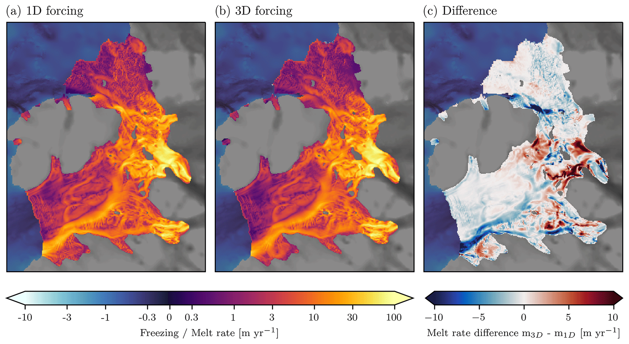
Figure A1 Impact of forcing on Crosson–Dotson melt rates. (a) Melt rates from 1D forcing, which are identical to Fig. 3d. (b) Melt rates from 3D forcing. (c) Difference between (a) and (b).

Notably, the melt patterns (Fig. A1a, b) show a strong similarity. From large to small scales, melt patterns and plumes are resolved regardless of the forcing field. These patterns are governed by the topography, which has a first-order impact on the basal melt patterns. The differences arise primarily in the high-melt region downstream of the Smith grounding zone (higher melt for 3D forcing) and the melt channels and shear zones (lower melt rates for 3D forcing). These differences arise due to the differences in the applied forcing fields, including the stratification therein. We note that a greater overlap between the two cases could be achieved if the 1D forcing profiles were derived directly from the 3D MITgcm fields. However, this comparison shows the difference between the simplest application of the model (idealised 1D forcing) and the most complex one (detailed 3D forcing). Although significant differences exist, the basal melt patterns are nearly identical, implying that the exact forcing has a second-order effect. A major exception to this is the average basal melt rate, which is strongly tied to the forcing applied.

The above analysis illustrates that basal melt patterns at the scale of the relatively small Crosson–Dotson Ice Shelf are predominantly governed by the ice shelf topography, rather than the distribution of heat and salt throughout the cavity. This conclusion may be less applicable to the larger Filchner–Ronne Ice shelf. Here, the spatial scales allow for a stronger horizontal non-uniformity in the distribution of warm and cold water masses throughout the cavity. Hence, an accurate 3D forcing may have a larger impact on the basal melt pattern of large ice shelves such as Filchner–Ronne.

Appendix B: Tuning

As described in the main text, we consider two parameters, C_d,top and D_min, as tuning parameters. The tuning is based on the Crosson–Dotson simulations with 3D forcing from MITgcm, averaged over the period 2003–2008. For both parameters, we apply a tuning procedure based on five tuning targets described below. The parameters are tuned for three horizontal resolutions, namely Δx=0.5, 1.0 and 2.0 km. We scale the horizontal viscosity and diffusion linearly with the resolution, leading to values A_h = K_h=25, 50 and 100 m² s⁻¹, respectively. These latter values were based on trial and error and are largely guided by numerical stability.

For each resolution, 16 simulations are performed with all combinations of $C_{\mathrm{d},\mathrm{top}}\in$ [0.8, 1.0, 1.2, and $\mathrm{1.4}\times {\mathrm{10}}^{-\mathrm{3}}$] and of D_min∈ [2, 4, 6, 8 m]. For each of these 16 simulations, the diagnostics described below are quantified. Based on the best fit to the tuning targets for each of the three resolutions, the optimal values of C_d,top and D_min are extracted.

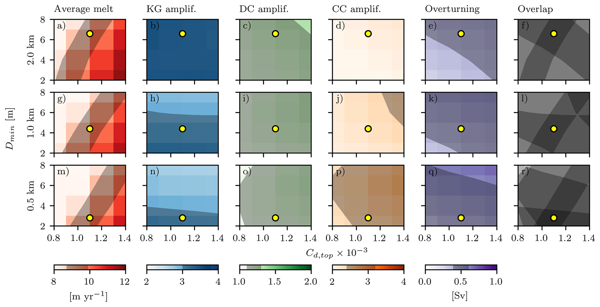
Figure B1 Parameter sensitivity test and tuning results. The three rows represent three horizontal resolutions (2.0, 1.0 and 0.5 km). Each column represents a diagnostic. Columns 2–4 denote the dimensionless melt amplification in the Kohler grounding zone (KG), the Dotson Channel (DC) and along the channel centreline (CC). The grey shading denotes the tuning targets based on observations. The last column (Overlap) displays the overlap of these grey-shaded regions, with darker colours indicating a better fit to observations. The yellow dots denote the chosen parameters for each resolution.

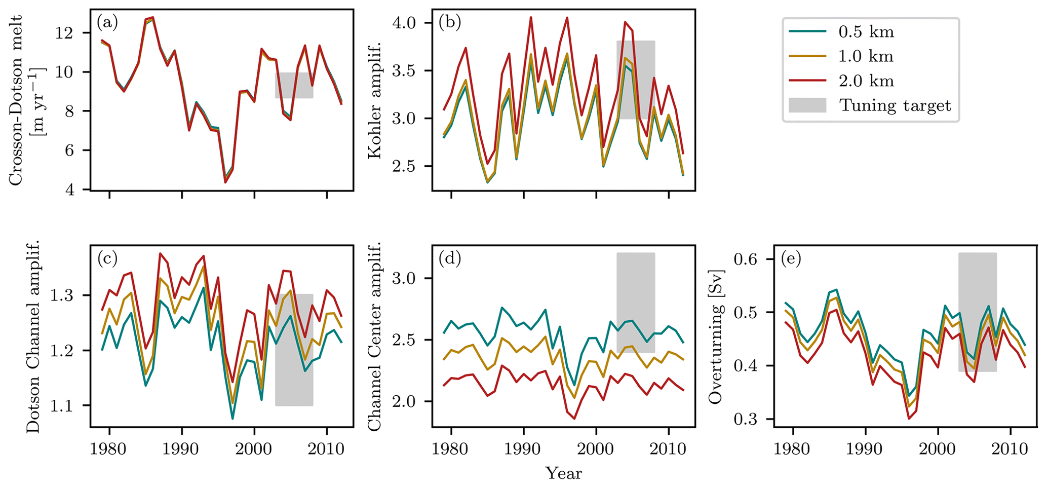
Figure B2 Time series of the main diagnostics for the Crosson–Dotson Ice Shelf (the same as in Fig. B1). For each year, the annual mean temperature and salinity fields from MITgcm are used to force LADDIE until steady state from a motionless initial state. The coloured lines again denote the different model resolutions. The grey regions denote the tuning targets, based on observations, applied to the period 2003–2008.

B1 Tuning targets

As tuning targets, we consider a range of five diagnostics. The average melt rate over the total Crosson–Dotson Ice Shelf is tuned to a range of 8.7–9.9 m yr⁻¹. This range is based on the average melt rate of 9.3±0.6 m yr⁻¹ derived from remote sensing observations over the period 2003–2008 by Rignot et al. (2013).

The following three diagnostics represent the spatial melt pattern: the melt rate in the Kohler grounding zone, the Dotson Channel and the centreline along the Dotson Channel (see Fig. 3 for the locations). The melt rates in these regions are tuned to remote sensing observations over a different period (2010–2016) in order to utilise the data of Gourmelen et al. (2017). To compensate for interannual variability, we tune the model to melt amplifications (regional melt divided by ice-shelf average melt), rather than the actual melt rates. These amplifications were found to be more robust on an interannual basis.

For the Dotson Channel and the centreline along this channel, tuning ranges are derived from the remote sensing observations over the period 2010–2016 by Gourmelen et al. (2017), equal to those presented in the main text. Melt amplifications are derived by dividing these regional melt rates by the Crosson–Dotson average melt rate of 6.89 m yr⁻¹ over 2010–2016 (Goldberg et al., 2019). Note that we follow Goldberg et al. (2019) and average melt rates by omitting negative values. This leads to regional melt amplifications in the Dotson Channel of 1.2 and along the channel centreline of 2.8. Without reported uncertainties in the data set, we are forced to prescribe arbitrary uncertainties. We apply tuning ranges of 1.1–1.3 and 2.4–3.2, respectively.

For the Kohler grounding zone, we combine estimates from the same remote sensing data set with estimates from radar observations over the comparable period 2010–2014 (Khazendar et al., 2016). The average melt rate over the Kohler grounding zone from remote sensing is 25.5 m yr⁻¹. From radar observations, this is 20.4 m yr⁻¹. Using these values as upper and lower bounds for the tuning range gives a range for the Kohler amplification of 3.0–3.8.

The fifth and last diagnostic used as a tuning target is the total overturning circulation. The overturning in LADDIE can be interpreted in two ways, dependent on the assumption of the fate of detrained water. If this water exits the cavity below the meltwater plume, it is part of the total overturning; if it recirculates in the cavity and re-enters the meltwater layer through entrainment, it is not. Here, we assume the former, and interpret the overturning as the integrated entrainment of ambient water. This volume flux, together with the small volume flux of meltwater, exits the meltwater layer through detrainment and outflow across the ice shelf front. Note that for Crosson–Dotson the contribution of detrainment is small and that the tuning is independent of the above interpretation. We extract observations from the years 2006, 2007 and 2011 during which melt rates were comparable to the period 2003–2008 (Jenkins et al., 2018). We take a tuning range based on the lowest and highest observations among these 3 years, leading to a range of 0.39–0.61 Sv.

B2 Tuning results

The tuning results are shown in Fig. B1, with the first five columns representing the five tuning targets and the three rows representing the three resolutions. The coloured shading displays the simulated diagnostic values. The grey-shaded zone in each panel marks the tuning range. In the sixth column, the overlap of the five tuning ranges is shown, with darker regions marking a better agreement with the tuning targets.

Based on this overlap, the optimal values for C_d,top and D_min are determined, marked by the yellow dots. For resolutions of 1.0 and 2.0 km, four of the five diagnostics fall within the tuning range, with the channel centreline (CC) being the exception. For the resolution of 0.5 km, all five tuning targets are met, and a full agreement was found between model and observations.

We find that we can choose the same optimal value for C_d,top for each resolution. This value of $\mathrm{1.1}\times {\mathrm{10}}^{-\mathrm{3}}$ is close to the value of $\mathrm{1.0}\times {\mathrm{10}}^{-\mathrm{3}}$ taken by previous studies (Jourdain et al., 2017; Mathiot et al., 2017). Keeping this same value of C_d,top for all resolutions, we find that differences in resolution – and correspondingly the viscosity A_h and diffusivity K_h – can be compensated for by varying D_min. Keeping the same parameter values, the average melt and the Kohler amplification decrease when the resolution is increased. Decreasing D_min reduces the thickness of the thermal barrier that the simulated layer forms between the warm ambient water and the ice shelf draft. The consequence is that a reduced value of D_min increases the average melt and the Kohler amplification, thus compensating for the increased resolution.

The single tuning target that cannot be obtained with all resolutions is the channel centreline (CC) amplification. The observed range of 2.4–3.2 can only be reproduced using a resolution of 0.5 km (Fig. B1p). While the melt amplification over the full width of the Dotson Channel can be reproduced with each resolution, the sharpness of the melt peak across this channel requires a high resolution and a low viscosity and diffusivity. This finding highlights the importance of high-resolution basal melt patterns. Forcing an ice shelf model with basal melt rates at a too coarse resolution may underestimate the thinning along the centreline of the channel. This can lead to an underestimation of the time it takes for the channel to “burn through” the ice shelf (e.g. Gourmelen et al., 2017). The optimal parameter values for each resolution are used throughout the current study for both Crosson–Dotson and Filchner–Ronne Ice Shelves.

In order to show the robustness of the tuning procedure to the interannual variability, we have performed simulations for each year between 1979 and 2012 using annual mean 3D forcing from the MITgcm simulations (Fig. B2). For the average melt (Fig. B2a), the interannual variability is strong and time periods must be selected carefully, as we have done. For the regional melt applications (Fig. B2b–d) and the overturning circulation (Fig. B2e), the interannual variability is comparable to the assessed uncertainty. Hence, the exact time period used to gather the tuning targets from observations is less important. Based on this, we are confident that the above tuning procedure is robust with respect to interannual variability.

Appendix C: Pine Island

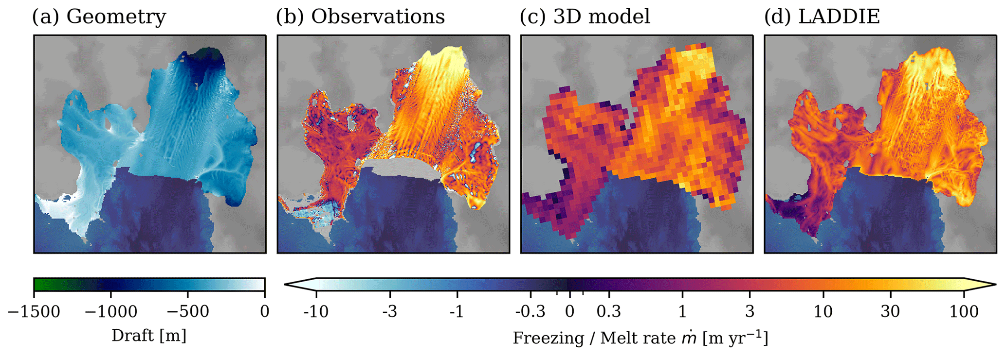
Figure C1 Geometry and basal melt for Pine Island Ice shelf: (a) geometry from BedMachine v2 (Morlighem et al., 2020), (b) observed basal melt rates from Shean et al. (2019), (c) 3D model output from MITgcm (Sect. 2.2.3), (d) results from LADDIE.

As additional model evaluation, we have included basal melt patterns for the Pine Island Ice Shelf (Fig. C1). This ice shelf resides near Crosson–Dotson in the warm Amundsen Sea Embayment.

The observations (Fig. C1b) are from Shean et al. (2019) using a method based on remote sensing comparable to that used for the Crosson–Dotson observations from Gourmelen et al. (2017). The 3D model output (Fig. C1c) is from the same MITgcm simulation over the same period as described in Sect. 2.2.3. LADDIE is configured with the same model tuning as Crosson–Dotson and Filchner–Ronne, at 500 m resolution. Its forcing is nearly identical to that of Crosson–Dotson, with the sole adaptation that the temperature at depth is set at 1.0 ^∘C and the thermocline depth is set at 450 m, mimicking the observations from Dutrieux et al. (2014). The simulation is run for a total of 30 model days, taking 23 CPU minutes.

The average melt rate simulated by LADDIE is 15.3 m yr⁻¹, in good agreement with observed estimates from Rignot et al. (2013) (16.2±1 m yr⁻¹) and from Shean et al. (2019) (13.1–14.9 m yr⁻¹, converted from Gt yr⁻¹ using the ice shelf area from Rignot et al., 2013). The total overturning circulation simulated by LADDIE is 0.34 Sv, which falls within the observed range of 0.25–0.40 Sv (Dutrieux et al., 2014). Based on these results, we conclude that the model tuning based on Crosson–Dotson is applicable to other warm ice shelves as well.

Besides the bulk numbers described above, a close agreement is found between the observed melt pattern (Fig. C1b) and the simulated melt patterns by MITgcm (Fig. C1c) and LADDIE (Fig. C1d). A major discrepancy is the deepest grounding zone, where both models simulate lower melt rates than the observed values, though the observations are uncertain in this region because the ice is not freely floating. A clear overlap between observations and LADDIE is found in the Y-shaped channel near the southern ice shelf front, where melt plumes with enhanced melt rates flow through the channel. In addition, a large number of meandering channels are observed and simulated in the centre of the ice shelf. These results illustrate that LADDIE simulates significantly more realistic melt patterns for Pine Island Ice Shelf than simpler basal melt parameterisations (Burgard et al., 2022).