The effect of partial dissolution on sea-ice chemical transport: a combined model–observational study using poly- and perfluoroalkylated substances (PFASs)

We investigate the effect of partial dissolution on the transport of chemicals in sea ice. Physically plausible mechanisms are added to a brine convection model that decouples chemicals from convecting brine. The model is evaluated against a recent observational dataset where a suite of qualitatively similar chemicals (poly- and perfluoroalkylated substances, PFASs) with quantitatively different physico-chemical properties were frozen into growing sea ice. With no decoupling the model performs poorly – underestimating the measured concentrations of high-chain-length PFASs. A decoupling scheme where PFASs are decoupled from salinity as a constant fraction of their brine concentration and a scheme where decoupling is proportional to the brine salinity give better performance and bring the model into reasonable agreement with observations. A scheme where the decoupling is proportional to the internal sea-ice surface area performs poorly. All decoupling schemes capture a general enrichment of longer-chained PFASs and can produce concentrations in the uppermost sea-ice layers above that of the underlying water concentration, as observed. Our results show that decoupling from convecting brine can enrich chemical concentrations in growing sea ice and can lead to bulk chemical concentrations greater than that of the liquid from which the sea ice is growing. Brine convection modelling is useful for predicting the dynamics of chemicals with more complex behaviour than sea salt, highlighting the potential of these modelling tools for a range of biogeochemical research areas.

1 Introduction

Sea ice is a complex, climatically important material and provides a habitat for a range of micro-organisms (Vancoppenolle et al., 2013). As sea ice cools, the internal, liquid brine becomes concentrated in solutes as more fresh, solid ice forms (e.g. Assur, 1958; Vancoppenolle et al., 2019). The increase in brine salinity raises the brine density (Maykut and Light, 1995; Cox and Weeks, 1988), which can drive brine convection (Notz and Worster, 2008) to supply nutrients (Fritsen et al., 1994) as well as harmful pollutants (Pućko et al., 2010a, b) to sea-ice communities. We can model salt dynamics and other conservative species (chemical species that are completely dissolved and exhibit similar behaviour to salt) in growing sea ice with good accuracy and precision (Rees Jones and Worster, 2014; Griewank and Notz, 2013; Turner et al., 2013; Thomas et al., 2020). However, modelling chemicals with non-conservative behaviour (chemical species with behaviour that deviates from salt due to physico-chemical or biological interactions within sea ice) has received less attention (e.g. Vancoppenolle et al., 2010; Zhou et al., 2013; Kotovitch et al., 2016). This problem has broad biogeochemical relevance, with gasses such as CO₂ (Tison et al., 2002) and CH₄ (Zhou et al., 2014), macro-nutrients (Vancoppenolle et al., 2010), iron (Lannuzel et al., 2016), and stable water isotopes (Eicken, 1998; Smith et al., 2012) all having potential to behave non-conservatively with respect to salinity in sea ice. A recent observational study gives us an opportunity to explore this problem in a systematic way. Garnett et al. (2021) measured the concentration profiles of a suite of 10 poly- and perfluoroalkylated substances (PFASs) as they froze into laboratory-grown sea ice. The measured PFASs share acidic functional groups (carboxylic and sulfonic acids) but exhibit differences in their carbon-chain lengths (ranging from 4 to 12) and their physico-chemical properties (see Table 1, where octanol–water partitioning coefficients vary by several orders of magnitude). Intriguingly, Garnett et al. (2021) found that short-chain PFASs (carbon-chain lengths <8) behaved similarly to the bulk salinity (conservatively), while long-chain PFASs (carbon-chain lengths ≥8) were enriched relative to the bulk salinity. Further, long-chained PFASs tended to be even more enriched in the shallowest measured sea-ice layer, and in some cases they had bulk concentrations greater than that of the underlying water. It is plausible that PFASs were not perfectly dissolved in sea-ice brine during these experiments. The extreme cold and high salinity of brine have the potential to drive solutes from solution, while the surface active properties of PFASs could cause them to stick to internal ice surfaces. Given that brine convection is the dominant process redistributing solutes in growing sea ice (Notz and Worster, 2009), we hypothesise that the physico-chemical properties of the PFASs have partially decoupled them from the convecting brine and that this decoupling has caused the observed deviations from conservative behaviour.

Here, we test that hypothesis by using observations of PFASs (Sect. 2.1) to evaluate a brine convection model (Sect. 2.2.1). We run three simulations that include plausible mechanisms of decoupling and tune each mechanism against the observations (Sect. 2.2.2). Comparing the model performance to the observations allows us to test our hypothesis and identify the likely factors controlling PFAS dynamics in our experimental system (Sect. 3). Finally, in Sect. 4 we provide insights into how brine convection parameterisations can be adapted to model non-conservative chemicals in sea ice.

2 Methods

2.1 Observations

The PFAS observations were collected during two sea-ice freeze experiments performed using the Roland von Glasow Air-Sea-Ice Chamber (Thomas et al., 2021) where sea ice was grown from NaCl water. Results and methods are presented in full in Garnett et al. (2021). Two experiments were conducted (Freeze-1: air temperature −35 ^∘C, 3 d, 17 cm final sea-ice thickness; Freeze-2: air temperature −18 ^∘C, 7 d, 26 cm final sea-ice thickness), with samples extracted using the Cottier et al. (1999) method at the end of the growth phase, sectioned vertically, and measured for bulk NaCl and PFAS concentrations (Table 1). Following Garnett et al. (2021) we omit the lowest sea-ice layer from our analysis due to a sampling bias, and we exclude one PFAS (6:2 fluorotelomer sulfonic acid) as the reported concentrations are described as “semi-quantitative”. We are left with measurements of bulk sea-ice concentration for NaCl and nine PFASs. The Freeze-1 and Freeze-2 depth profiles were subsampled into nine and eight vertical layers, respectively, giving 17 measured samples. We therefore have 17 measurements of bulk concentration, c_si, for NaCl and 153 for PFASs. The concentration of the experiment water was measured three times when the system was fully liquid, and we use the mean and standard deviation of these as the concentration before freeze-up, c_o, and uncertainty in that concentration, δ(c_o), respectively. The uncertainty in a single measurement, δ(c_si), is taken to be the median standard deviation of the measurements of the fully liquid ocean because these have repeat samples. We normalise the concentration of NaCl and each PFAS to c_o and estimate the uncertainty in the normalised concentration by propagation of the measurement uncertainty. Normalising the concentrations allows us to compare the behaviour of PFASs to each other and to NaCl. A full list of chemicals and selected key physico-chemical properties is given in Table 1.

Table 1 PFASs used in this study. Initial water concentrations, c_o, and analytical uncertainties, δ(c_o) and δ(c_si), were taken from Garnett et al. (2021). N_C is the carbon-chain length; log₁₀K_OW is a measure of partitioning between an organic and aqueous phase.^* The best tuning parameters for each decoupling method (α, Sect. 2.2.2) are also given.

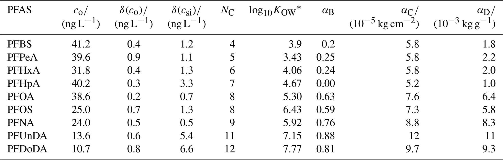
${}^{*}{K}_{\mathrm{OW}}=\frac{c_{\mathrm{octanol}}}{c_{\mathrm{water}}}$, where c_octanol and c_water are the concentrations of a PFAS dissolved in octanol and water, respectively. We present log₁₀K_OW for readability. Values were gathered from Smith et al. (2016).

2.2 Modelling

2.2.1 Model set-up

The model used was previously presented in Thomas et al. (2020), where brine dynamics parameterisations (Rees Jones and Worster, 2014; Griewank and Notz, 2013; Turner et al., 2013) based on Rayleigh number physics (Wells et al., 2011) were shown to perform well. The model has been used on several occasions to model tracers assumed to be perfectly dissolved in sea-ice brine (Thomas et al., 2020, 2021; Garnett et al., 2019), and it has been used to investigate the sensitivity to imperfect dissolution for rhodamine (Thomas et al., 2020). We used the brine convection parameterisation presented by Griewank and Notz (2013) because it has a set of well-evaluated tuning parameters, independent of our experimental system (Griewank and Notz, 2015), that allow us to test the robustness of our results to tuning (Sect. 4 and Supplement). We tuned the parameterisation by varying the critical Rayleigh number, Ra_c, and desalination strength, ϵ, and evaluated the pairs using the bias and mean absolute deviation between the modelled and measured salinity profiles. We chose the pair Ra_c=4.69 and ϵ=0.00438 kg (m³ s)⁻¹, which gave a bias of less than 1 % and a weighted mean absolute deviation of 4 % when compared to the 17 measurements of sea-ice bulk salinity. The model is initialised such that each sea-ice layer has the same bulk salinity and PFAS concentration as the underlying water, so the initial normalised concentration profile is identical for NaCl and each PFAS. Freeze-1 and Freeze-2 are modelled separately using temperature profiles and sea-ice thickness measured in each experiment (presented previously in Garnett et al., 2019). The model has 50 layers and a time step of 5 min. Chemicals are advected using

$$\begin{array}{}\text{(1)}& {\displaystyle \frac{\partial c_{\mathrm{si}}}{\partial t}}=-w{\displaystyle \frac{\partial c_{\mathrm{br}}}{\partial z}},\end{array}$$

where w is the upward brine velocity calculated using the Griewank and Notz (2015) parameterisation as described in Thomas et al. (2020) and c_br is the concentration of the chemical dissolved in brine. For salinity, c_br is a function of the local temperature (Weast, 1971). For PFASs,

$$\begin{array}{}\text{(2)}& {\displaystyle \frac{c_{\mathrm{si}}}{\mathit{\varphi }}}=c_{\mathrm{br}}+c_{\mathrm{s}},\end{array}$$

where ϕ is the brine fraction. Equation (2) expresses the choice of splitting the dissolved-in-brine PFAS pool into a mobile phase (c_br) and a stationary phase (c_s). For salt or other fully mobile tracers, c_s is zero, reducing to $c_{\mathrm{br}}=\frac{c_{\mathrm{si}}}{\mathit{\varphi }}$, which is normally used (e.g. Cox and Weeks, 1988).

2.2.2 Methods of decoupling

For PFASs, c_s may be non-zero because of decoupling processes, where the term “decoupling” here refers to a physical or chemical (or in other systems biological) process which removes PFASs from the free dissolved phase, thus preventing advection alongside brine in our model. We express the stationary phase as a fraction of the total brine concentration such that

$$\begin{array}{}\text{(3)}& c_{\mathrm{s}}=\mathit{\gamma }{c}_{\mathrm{si}}/\mathit{\varphi },\end{array}$$

where γ is decoupling parameter, with the condition that c_s⩽c_br. As a first step (Method A), we model PFASs with no decoupling such that

$$\begin{array}{}\text{(4)}& \mathit{\gamma }=\mathrm{0}.\end{array}$$

Method A models PFASs using the same numerical scheme as salinity, is the obvious choice for modelling solute dynamics, and serves as quality control because PFASs should behave identically to NaCl.

Our simplest decoupling mechanism (Method B) alters the concentration of PFASs in brine as a constant fraction.

$$\begin{array}{}\text{(5)}& \mathit{\gamma }={\mathit{\alpha }}_{\mathrm{B}},\end{array}$$

where α_B is a free tuning parameter derived separately for each PFAS. Next (Method C), motivated by the surface active properties of PFASs, which tend to adsorb to surfaces (Grannas et al., 2013), the brine PFAS was decoupled from the stationary phase proportionately to the internal sea-ice surface area:

$$\begin{array}{}\text{(6)}& \mathit{\gamma }={\mathit{\alpha }}_{\mathrm{C}}{A}_{\mathrm{si}}\left(\mathit{\theta }\right),\end{array}$$

where α_C is a free tuning parameter and A_si(θ) is the internal sea-ice surface area as a function of the temperature, θ, as given by Krembs et al. (2000) for columnar sea ice (see Thomas et al., 2020, their Eq. B1).

Finally (Method D), we decouple the brine PFAS concentration as a function of brine salinity, motivated by the tendency of high-ionic-strength solutions to drive out solutes such as PFASs (e.g. Freire et al., 2005):

$$\begin{array}{}\text{(7)}& \mathit{\gamma }={\mathit{\alpha }}_{\mathrm{D}}{S}_{\mathrm{br}}\left(\mathit{\theta }\right),\end{array}$$

where α_D is a free tuning parameter.

While the brine salinity (Rees Jones and Worster, 2014; Weast, 1971) and internal surface area (Krembs et al., 2000) are both functions of temperature, the functional form is approximately opposite, with brine salinity decreasing and surface area increasing with temperature.

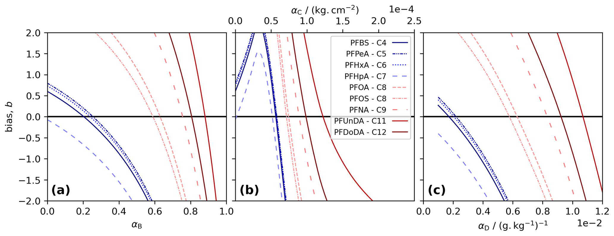
Figure 1 Model tuning for each PFAS. The bias, b, was calculated as the sum of the difference between measurements and co-located model layers in three tuning runs. Each panel shows results for a different decoupling method: (a) simple decoupling, tuned using α_B; (b) surface area adsorption, tuned using α_C; and (c) salinity-mediated decoupling, tuned using α_D. The best-performing α gives the b value closest to 0 (black line).

We choose α, for Methods B to D and for each PFAS, by running the model using 100 values of α and picking the best-performing α. The performance was quantified using the bias, b, taken to be the sum of the residuals for each measurement relative to the co-located model depth at the end of the simulation. The best-performing α gives the b value closest to 0. For each method, short-chained PFASs tend to produce lower α, and the two longest-chained PFASs always give the highest α (Table 1, Fig. 1).

3 Results

With no decoupling (Method A, using Eq. 4) we see a systematic difference between the measured and modelled PFAS concentrations (Figs. 2a to c and 3). NaCl concentrations are captured well (following salinity tuning in Sect. 2.2.1). All of the PFAS model lines are identical to that of NaCl, but the observations shift to higher concentrations as the carbon-chain length moves from low to high, and some of the measured concentrations in the upper layer are above 1 (Fig. 2a and b). This shift is reflected in the correlation of measured and modelled concentrations, with lower chain lengths and NaCl clustered around the 1-to-1 line (perfect model behaviour) but with longer chain lengths tending to lie above the 1-to-1 line (Fig. 2c). We use a weighted least squares (WLS) regression of modelled vs. measured concentration to quantify the model performance, using the inverse variance for each measurement as the weights. Good model behaviour is taken to be a gradient, k, consistent with 1 (ideally within a standard error and at a minimum within 95 % confidence intervals, 95 % CI) and a high coefficient of determination, r². The variability in the observations is barely captured (r²=0.15), with the highest model concentrations less than 0.5 and the observations systematically above this for some of the long-chained PFASs. Though the gradient is consistent with 1 ($k=\mathrm{0.93}\pm \mathrm{0.16},\mathrm{95}\mathit{\%}$ CI [0.57, 1.28]), the uncertainty is such that k is poorly constrained. This regression is poor and motivates further model development.

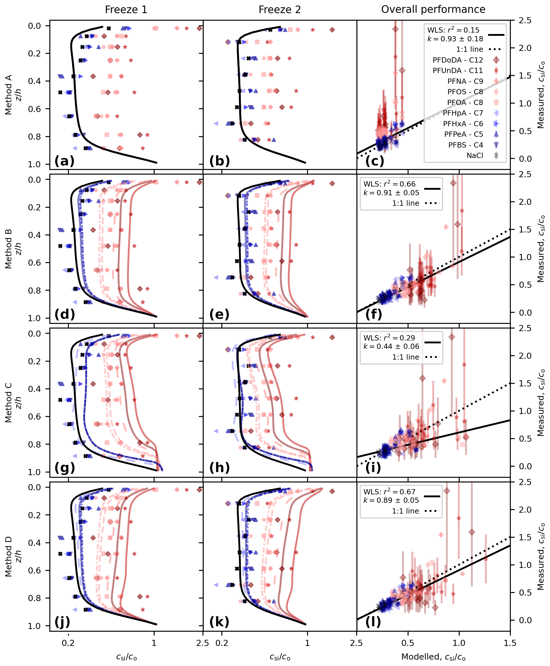
Figure 2 Comparison of modelled and measured concentration for the following: Method A, perfectly dissolved chemicals (a, b, c); Method B, simple decoupling (d, e, f); Method C, surface area adsorption (g, h, i); and Method D, salinity-mediated decoupling (j, k, l). Depth profiles are shown for Freeze-1 (a, d, g, j) and Freeze-2 (b, e, h, k). Modelled vs. measured concentrations are shown in panels (c), (f), (i), and (l), alongside the best-fit weighted least squares (WLS) regression (black line, gradient k with 1 standard error and coefficient of determination r² shown in legend) and the theoretical 1-to-1 line for perfect model behaviour (dotted black line). The concentration for the profiles is given on a log scale to highlight separation between the profiles.

Method B (using Eq. 5) shifts the modelled PFAS concentrations higher (Fig. 2d to f). Model lines for the PFAS profiles can now be distinguished from each other and from NaCl but remain similar in shape. Longer-chained PFASs have moved further from the NaCl profile, and for PFUnDA and PFDoDA (chain lengths 11 and 12, respectively), concentrations rise above 1 near the upper interface. The regression is dramatically improved, with r²=0.66 and $k=\mathrm{0.91}\pm \mathrm{0.05}$ (95 % CI [0.80, 1.01]).

Surface-area-mediated decoupling (Method C, using Eq. 6) also shifts the modelled PFAS concentrations higher (Fig. 2g to i). The profile shape is different to that of Method B. Moving from the lower interface up, we see a region of constant PFAS concentration, then a decline in concentration, a region of near-constant concentration, and finally an increase near the upper interface (see also Fig. 3). Method C overestimates PFASs in the lower sea ice, and the regression is poor (r²=0.29, $k=\mathrm{0.44}\pm \mathrm{0.06}$, 95 % CI [0.33, 0.55]).

Brine-salinity-mediated decoupling (Method D, using Eq. 7), as with Methods B and C, shifts the modelled PFAS concentrations higher (Fig. 2j to l). Moving upwards from the lower interface, the concentration decreases sharply, rises steadily until near the upper interface, and then increases sharply towards the upper interface. The largest upper-layer concentrations are predicted by Method D, reaching 1.25. The Method D regression (r²=0.67, $k=\mathrm{0.89}\pm \mathrm{0.05}$, 95 % CI [0.79, 0.99]) performs better than Methods A and C. Method D performs marginally worse than Method B with regards to gradient but captures slightly more of the variability.

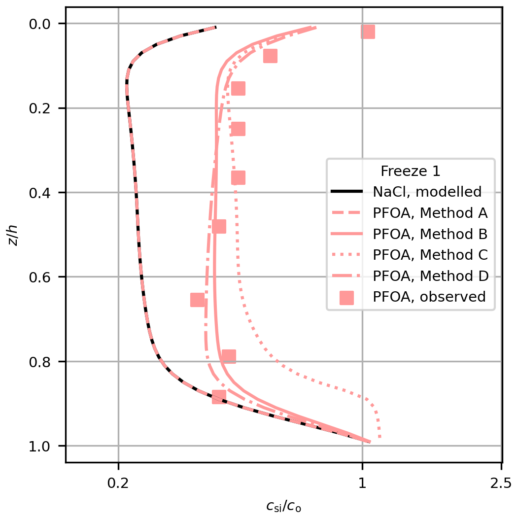
Figure 3 Comparison of modelled (lines) and measured (squares) PFOA concentration in Freeze-1 for each method. Modelled NaCl is also shown (black line).

Methods C and D provide further insights into the mechanism of the decoupling. To explore the differences between the methods, we take just one profile (PFOA for Freeze-1) and show the performance of each method alongside the observations (Fig. 3). The change in bulk PFAS concentration is proportional to the vertical brine PFAS gradient when using the Griewank and Notz (2013) scheme (Eq. 1). Decoupling by surface area (Method C) performed worse than Methods B and D, failing to simultaneously reproduce the shape and magnitude of the PFAS observations, particularly near the lower interface. Method C differs from Method B by including a dependence of the decoupling on the internal sea-ice surface area, which increases non-linearly with temperature (Krembs et al., 2000). Towards the base of the sea ice the PFASs are nearly completely decoupled due to the high surface area, so the vertical brine PFAS concentration gradient is near 0, causing little change in bulk PFAS concentration with brine convection. Bulk concentration is therefore fixed at near the underlying water concentration until the sea ice grows and cools and the surface area decreases (Fig. 3). Method C cannot simulate the general increase in PFAS concentrations without unrealistically distorting their distribution. These results indicate that surface-active properties linked to the internal surface area of the sea ice were unlikely to have controlled the behaviour of PFASs in these experiments.

Method D (Eq. 7) differs from Method B (Eq. 5) by including an explicit dependence of the decoupling on S_br (which decreases non-linearly with increasing temperature). With Method D, higher S_br near the upper interface reduces the PFAS concentrations in brine mostly in the upper layers, causing preferential retention of PFASs higher in the sea ice (Fig. 3). Despite this, Methods B and D are similar in terms of their profile shape and quantitative performance. This similarity arises because Method B also includes a (implicit) dependence on S_br. The product $\mathit{\gamma }{c}_{\mathrm{si}}/\mathit{\varphi }$ (Eq. 2) increases with S_br (for both methods) because ϕ linearly scales with S_br. After tuning, both methods simulate similar dynamics. The gradient of the modelled concentrations using Method D regressed against the measurements is just inconsistent with 1 at 95 % confidence. However, given the improvement in model performance with Method D relative to Method A and the similar performance between Method B (which produced a gradient consistent with 1) and Method D, our results are consistent with increased S_br driving PFASs out of solution being an important decoupling mechanism in our study. Both methods are able to bring the model into reasonable agreement with the available observations, and further measurements would be needed to robustly distinguish between Methods B and D.

We return now to our hypothesis that, in the experiments of Garnett et al. (2021), the physico-chemical properties of the PFASs decoupled them from convecting brine, resulting in deviations from behaviour that is conservative with regards to salinity. The results for Method B are consistent with our hypothesis. The simple decoupling, implemented in a brine convection model, was sufficient to bring the modelled concentrations into quantitative agreement with the observations. Further, decoupling within brine and brine convection (particularly Method D) gave PFAS concentrations significantly above that of the underlying water and similar to the observations.

4 Discussion

How general are our results? How robust is the brine convection tuning, and can our methods be applied to thicker sea ice, other PFASs, and other chemicals? We tuned the model for this set of observations using NaCl measurements from the same samples as the PFAS measurements, which were extracted using the Cottier et al. (1999) method. While this method is the best sampling method we are aware of for young sea ice, retaining more brine than cores, it may still underestimate the sea-ice bulk salinity. A brine-loss-driven sampling bias may impact PFASs differently to salt. If PFASs were preferentially retained, the observed enrichment in the sea ice would overestimate the in situ value. Also, tuning to samples affected by this bias would cause the tuning parameters to give too much desalination (Thomas et al., 2021). Griewank and Notz (2015) present tuning parameters that perform well against observations when redistributing salt in simulations of Arctic sea ice, and we test the robustness of our tuning by running a parallel set of model runs and analyses using the Griewank and Notz (2015) tuning parameters (Supplement, Figs. 1 and 2). Our conclusions are robust, with Method A performing poorly, Methods B and D improving model performance, and Method C performing poorly, and longer-chained PFASs generally give larger values of α. The Griewank and Notz (2015) parameters perform worse than those derived for this study, but this is unsurprising and does not reflect poorly on the Griewank and Notz (2015) parameters, given we tuned the model to salinity measurements made alongside the PFAS measurements.

Turning to the application of these results to thicker sea ice, we expect our results to generalise to thicker growing sea ice because brine convection will remain the dominant redistributor of solutes (Notz and Worster, 2009), with the caveat that the increased complexity in natural environments (transient periods of melt conditions, cracks in the sea ice, flooding of the surface) could significantly alter the redistribution of solutes beyond that driven by brine convection.

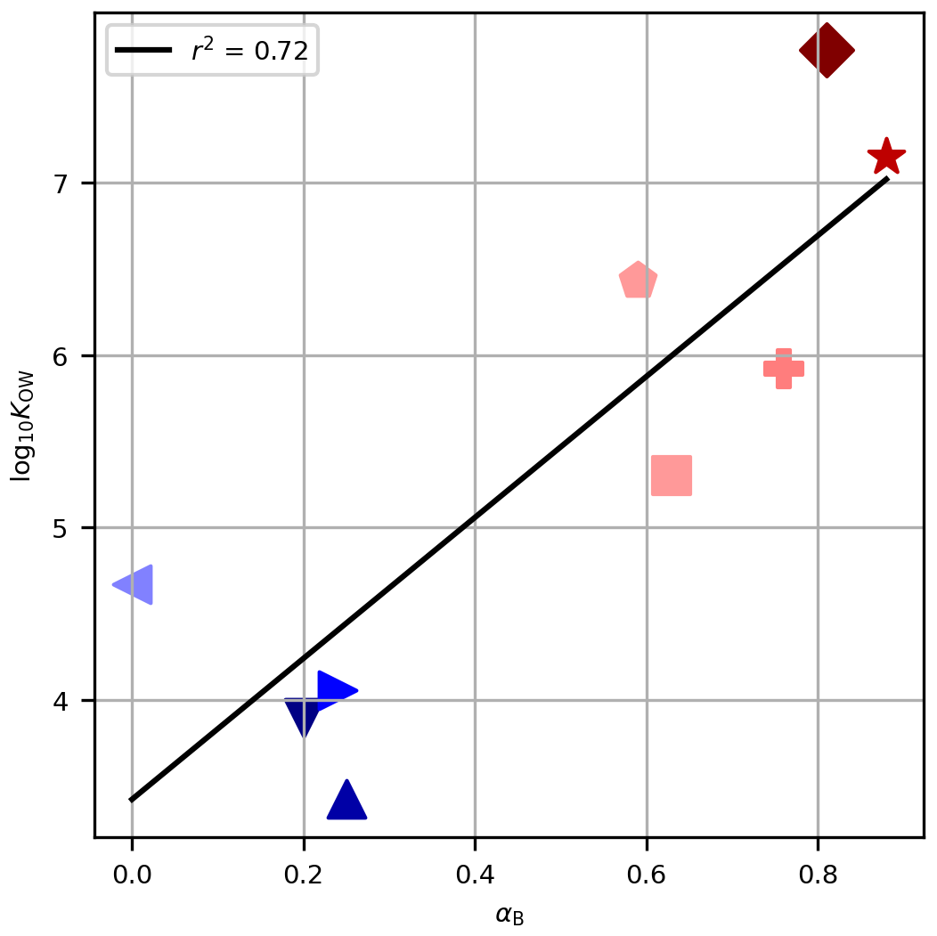
Figure 4 The octanol–water partitioning coefficient, log₁₀K_OW, against the derived tuning parameter for Method B, α_B, for each PFAS. Symbols are as in Fig. 2. The black line shows the linear regression of log₁₀K_OW against α_B, and the coefficient of determination is given in the legend.

For Method B (which performed satisfactorily) the tuning parameters derived for the PFASs, α_B, are associated with the physico-chemical properties, as evidenced by the non-random ordering of α_B with chain length (Table 1, Fig. 1). The partitioning coefficients presented (log₁₀K_OW in Table 1) tend to increase with chain length and are correlated with α_B (Fig. 4, r²=0.72, p<0.05). This result builds confidence that our tuning parameters reflect real physico-chemical properties of the studied PFASs (though we acknowledge that organic–aqueous partitioning is of only indirect relevance to our experimental system). We also calculated this correlation for α_D (which also performed well) and for α_B and α_D against N_C (not shown). The correlations are all significant at 95 % confidence and range from r²=0.70 to r²=0.81. In our experimental system, with close-to-neutral pH, all PFASs in this study exist in their anionic form as conjugate bases. We therefore have some confidence that, for PFASs not investigated here, taking the tuning parameter for the nearest chain length would be a useful approximation in natural seawater environments. For other chemicals, the different physico-chemical properties would necessitate re-tuning and possibly different functional forms for decoupling, but the frameworks proposed here would be a useful starting point.

This study focused on PFASs, which are large organic pollutants, but the implications are more general. Many chemicals of interest behave differently to sea salt during sea-ice growth. Ammonia (Hoog et al., 2007), helium, and neon (Hood et al., 1998; Namiot and Bukhgalter, 1965) are partially incorporated within the ice matrix, isotopologues of water fractionate at ice–liquid interfaces (Lehmann and Siegenthaler, 1991), nutrients are consumed and remineralised (Vancoppenolle et al., 2010; Fritsen et al., 1994), gasses effervesce to bubbles and float upwards (Zhou et al., 2014; Kotovitch et al., 2016), and exopolymeric substances stick to internal surfaces (Krembs et al., 2011). We show here that quantitative agreement can be achieved for non-conservative chemicals in growing sea ice using brine convection modelling, highlighting the usefulness of these numerical tools to a range of biogeochemical sea-ice research areas.

5 Conclusions

A sea-ice brine convection model can reproduce observations of poly- and perfluoroalkylated substances (PFASs) freezing into sea ice, providing a term is introduced that partially decouples PFASs from the moving brine. PFASs with longer carbon chains were enriched with respect to salinity, sometimes to levels above the underlying water, in observations. Larger decoupling parameters were required to simulate this behaviour. Decoupling methods with primary dependence on the brine salinity performed well and outperformed a decoupling method that depended on the internal sea-ice surface area. Our results demonstrate that brine convection models are powerful tools beyond predicting sea-ice salinity. Complex, biogeochemical problems can benefit from the accurate, physically based advection of brine predicted by current parameterisations.