Foehn winds at Pine Island Glacier and their role in ice changes

Pine Island Glacier (PIG) has recently experienced increased ice loss that has mostly been attributed to basal melt and ocean ice dynamics. However, atmospheric forcing also plays a role in the ice mass budget, as besides lower-latitude warm air intrusions, the steeply sloping terrain that surrounds the glacier promotes frequent Foehn winds. An investigation of 41 years of reanalysis data reveals that Foehn occurs more frequently from June to October, with Foehn episodes typically lasting about 5 to 9 h. An analysis of the surface mass balance indicated that their largest impact is on the surface sublimation, which is increased by about 1.43 mm water equivalent (w.e.) per day with respect to no-Foehn events. Blowing snow makes roughly the same contribution as snowfall, around 0.34–0.36 mm w.e. d⁻¹, but with the opposite sign. The melting rate is 3 orders of magnitude smaller than the surface sublimation rate. The negative phase of the Antarctic oscillation and the positive phase of the Southern Annular Mode promote the occurrence of Foehn at PIG. A particularly strong event took place on 9–11 November 2011, when 10 m winds speeds in excess of 20 m s⁻¹ led to downward sensible heat fluxes higher than 75 W m⁻² as they descended the mountainous terrain. Surface sublimation and blowing-snow sublimation dominated the surface mass balance, with magnitudes of up to 0.13 mm w.e. h⁻¹. Satellite data indicated an hourly surface melting area exceeding 100 km². Our results stress the importance of the atmospheric forcing on the ice mass balance at PIG.

1 Introduction

The West Antarctic Ice Sheet and its marine-terminating ice shelves have been thinning rapidly in the last few decades, contributing to roughly 10 % of the observed global mean sea level rise (Jenkins et al., 2010; Smith et al., 2020). A collapse of the West Antarctic Ice Sheet alone is estimated to lead to a 3 m rise in the global sea level (Bamber et al., 2009), and model simulations suggest it can be initiated by an ocean warming of approximately 1.2 ^∘C (Rosier et al., 2021). One of the main contributors to the ice loss in West Antarctica is Pine Island Glacier (PIG; see Fig. 1a), which is presently Antarctica's single largest contributor to sea level rise (Favier et al., 2014; Joughin et al., 2021; Lhermitte et al., 2021). Over the last 2 decades, PIG has lost more than a trillion tonnes of ice, which corresponds to a roughly 3 mm rise in sea level (De Rydt et al., 2021). Satellite images indicate a jump in the average volume loss rate around PIG from roughly 2.6 in 1995 to 10.1 km³ yr⁻¹ in 2006 (Wingham et al., 2009), with recent studies stressing a further speedup of ice loss since 2017 (Joughin et al., 2021; Lhermitte et al., 2021; Nilsson et al., 2022). In fact, Li et al. (2022) reported a decrease in elevation around PIG, as estimated from satellite measurements, at a rate of approximately −2 ± 0.04 m yr⁻¹ from 2016 to 2019. Satellite data indicate an ice velocity magnitude in excess of 200 m yr⁻¹ over a broad region (Fig. 1a), with peak values higher than 4.5 km yr⁻¹ (Liu et al., 2022). The ice loss at PIG can be seen by the rapid retreat of the ice front (Fig. 1b), particularly since 2015, with major calving events taking place in October–November 2018 and February 2020 (Liu et al., 2022; Lhermitte et al., 2021).

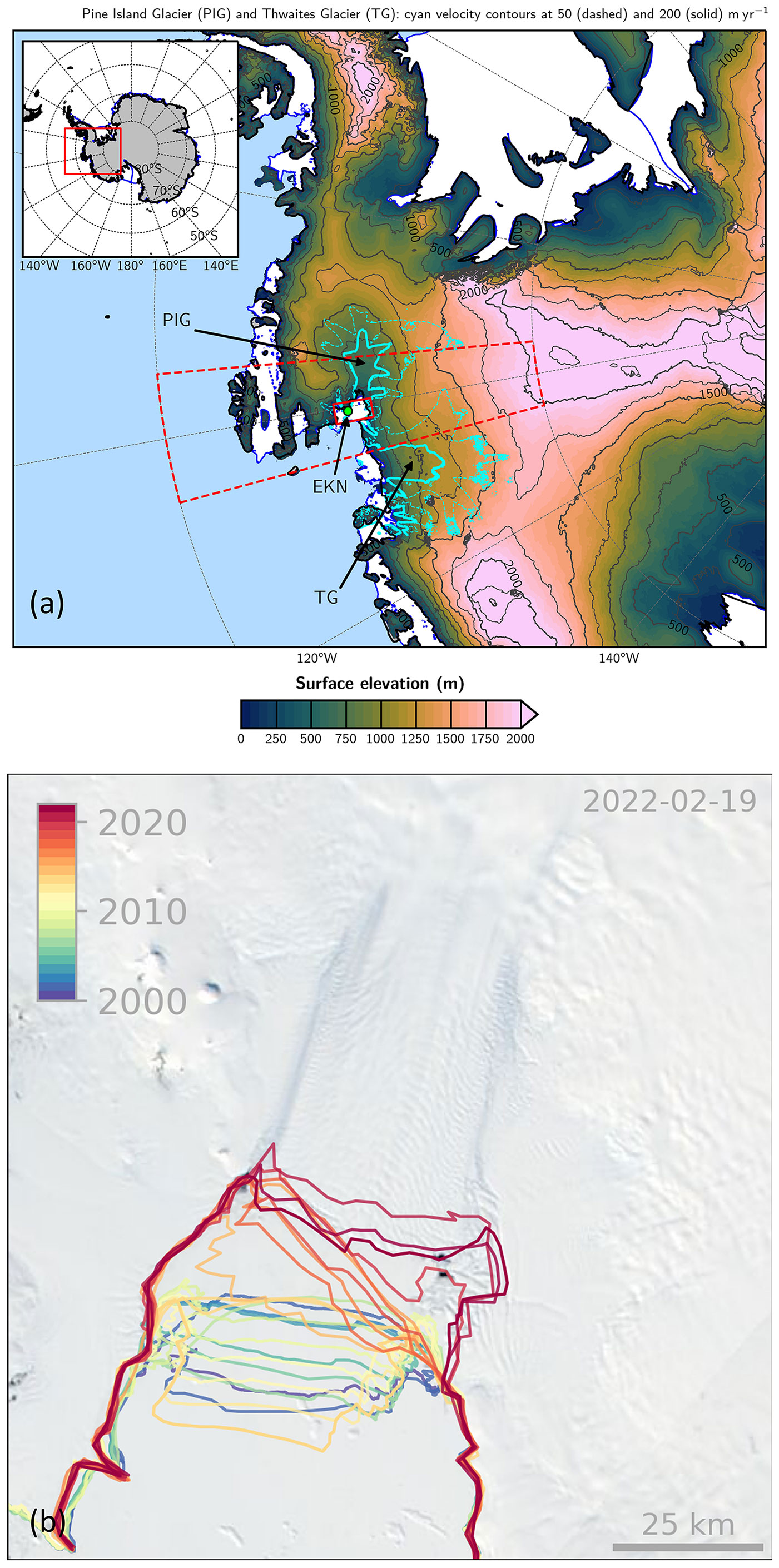
Figure 1 Pine Island Glacier (PIG) and surroundings. (a) Digital elevation map (DEM) at 1 km resolution, constructed using data for March 1994–January 1995 and February 2003–March 2008, showing PIG and Thwaites Glacier (TG). The shading and the black contours show the surface elevation (m) contoured every 500 m and labelled every 1000 m, while the regions where the ice velocity is equal to 50 and 200 m yr⁻¹ are denoted by the dashed and solid cyan contours, respectively. The ice velocities are estimated using data from the National Snow and Ice Data Center (NSIDC; Rignot et al., 2017) for 1996–2016. The blue line highlights the ice shelf borders. The solid red rectangle represents the domain over which the averaging is performed for the time series in Fig. 7 (−75.5 to −74.5^∘ S, −101.5 to −99.5^∘ W), whereas the dashed red rectangle highlights the domain used in Figs. 3–4 (80 to 70^∘ S, 105 to 95^∘ W). The location of the Evans Knoll weather station (−74.85^∘ S, −100.404^∘ W) is given by the green circle. The red square in the inlet gives the location of the study domain. (b) The 19 February 2022 MODIS satellite image of PIG with an overlay of historical calving fronts since 2000.

The melting around PIG has been attributed mostly to basal melt and ocean ice dynamics (Webber et al., 2017; De Rydt et al., 2021; Joughin et al., 2021). While ocean dynamics likely account for most of the observed ice loss, atmospheric forcing may also be important in modulating PIG ice loss, as has been shown recently to be the case elsewhere in the continent (e.g. Francis et al., 2021, 2022a; Greene et al., 2022). Besides atmospheric rivers (Willie et al., 2021; Francis et al., 2020) and associated surface radiative warming, one of the meteorological phenomena that can foster ice damage around Antarctica is Foehn winds (Elvidge and Renfrew, 2016; Ghiz et al., 2021). The word Foehn, which means “hair dryer” in German, refers to the warm and dry winds that descend on the lee side of a mountain range. Foehn effects can trigger surface melting and snow or ice sublimation (Bell et al., 2018), with melting being less likely as the low humidities during Foehn episodes cause large latent heat losses from the snowpack and hence prevent its warming. Additionally, Foehn winds can foster calving events (Miles et al., 2017), as an offshore wind direction, combined with ocean swells, aids in the breakup and subsequent drifting of newly formed icebergs (Francis et al., 2022a).

Several studies have reported the occurrence of Foehn around Antarctica, such as in the Ross Sea (e.g. Speirs et al., 2013; Zou et al., 2021a, b), at PIG (Djoumna and Holland, 2021), in the Vestfold Hills in East Antarctica (Gehring et al., 2022) and in the Antarctic Peninsula (e.g. Laffin et al., 2021). Zou et al. (2021a, b) investigated the processes behind four major melting events at the Ross Ice Shelf. In three of the four cases, Foehn warming occurred for more than 40 % of the melting period, causing a 2–4 ^∘C increase in surface temperature. The authors concluded that Foehn can be an important contributor to surface melting in Antarctica, which can increase the effects of warm and moist air advection. Djoumna and Holland (2021) reported Foehn conditions around PIG during March 2013 after the onset of a warm air intrusion associated with an atmospheric river. The combination of warm and moist air advection from lower latitudes and Foehn winds likely explains the record temperature of 17.5 ^∘C observed at the northern tip of the Antarctic Peninsula on 24 March 2015 (Bozkurt et al., 2018). A region in Antarctica particularly prone to Foehn effects are the McMurdo Dry Valleys. Speirs et al. (2013) presented a 20-year climatology of Foehn events at this site from weather station data. They reported positive trends for all seasons during 1999–2008, with a larger magnitude being present in winter when the large-scale dynamics favour the occurrence of Foehn. The role of Foehn winds in the disintegration and collapse of the Larsen Ice Shelf A, Larsen Ice Shelf B and Larsen Ice Shelf C on the Antarctic Peninsula in 1995, 2002 and 2017, respectively, has been widely reported (Massom et al., 2018). In fact, during periods of strong westerlies, the warmer and more moist maritime air is forced to rise over the mountains in the western Antarctic Peninsula and warms and dries out on the lee side, generating frequent Foehn events over the ice shelves on the eastern side of the peninsula (Laffin et al., 2021). The complex terrain around PIG (Fig. 1a) favours Foehn wind occurrence there as well.

Despite major advances in the understanding of the Antarctic surface mass balance in recent decades, there are still major uncertainties (e.g. The IMBIE Team, 2018), particularly in areas that are prone to ice loss such as PIG (Kowalewski et al., 2021). An important process for the surface mass balance is snow evaporation or sublimation (Das et al., 2013; Mottram et al., 2021), which is typically difficult to detect from observations given its nature. Even though Foehn events are believed to play an important role in the surface mass loss around Antarctica (Ghiz et al., 2021), the underlying processes remain unclear. Moreover, no study has examined the occurrence of Foehn on a longer timescale over PIG, even though it is expected to have a significant impact given the steep topography in the region (Fig. 1a). Hence, it is vital to quantify the occurrence of Foehn episodes so as to better understand their role in ice loss through melting and/or sublimation. This is achieved in the present work, where the occurrence of Foehn at PIG and its role in the surface mass balance is investigated using a state-of-the-art reanalysis dataset, satellite imagery and in situ measurements.

The remainder of the paper is organised as follows. In Sect. 2, the datasets used in this work, the Foehn detection algorithm employed and how the different terms in the surface mass balance are quantified are all described. Section 3 provides a discussion of the occurrence and trends of Foehn over PIG and its impacts on the surface mass balance. In Sect. 4 the focus is on the large-scale conditions that promote the occurrence of Foehn, while a case study in November 2011 is discussed in Sect. 5. Section 6 summarises the main findings of the study.

2 Datasets and methodology

2.1 Observational and reanalysis datasets

The main dataset used in this study uses the ERA-5 reanalysis data (Hersbach et al., 2020), which are available on an hourly basis and on a 0.25^∘ × 0.25^∘ (∼ 27 km) grid from 1950 to present. Both hourly pressure level (Hersbach et al., 2018a) and surface (Hersbach et al., 2018b) data are considered in this work for the period 1980–2020. ERA-5 is one of the best-performing reanalysis datasets around Antarctica in comparison with station observations (as noted by, e.g. Gossart et al., 2019).

The 1 km × 1 km dataset used for the digital elevation model of Pine Island Glacier (PIG) and the surrounding region combines measurements collected by the European Remote Sensing Satellite-1 (ERS-1) satellite radar altimeter from March 1994 to January 1995 and the Ice, Cloud, and land Elevation Satellite (ICESat) geosciences laser altimeter system from February 2003 to March 2008 (Bamber et al., 2009). The ice velocity for PIG and Thwaites Glacier is estimated from a combination of satellite interferometric and synthetic-aperture radar systems and is available at a 450 m spatial resolution from 1996 to 2016 (Mouginot et al., 2017b). Sentinel 2 satellite data, downloaded from Copernicus website (Copernicus, 2022), are used to extract the sea ice front at PIG for 2000–2022.

Surface radiation fluxes from the Clouds and Earth's Radiant Energy System (CERES; Doelling et al., 2013, 2016) dataset are available on an hourly basis at 1^∘ × 1^∘ resolution from March 2000 to present. The CERES product used here is the SYN1deg – Level 3, which is freely available online (NASA/LARC/SD/ASDC, 2017) and is downloaded for the period 3–14 November 2011 that corresponds to the case study discussed in Sect. 5.

The 10 min air temperature observations at the Evans Knoll station (−74.85^∘ S, −100.404^∘ W; 188 m a.s.l.), located just to the northeast of PIG (green circle in Fig. 1a), are freely available at the Antarctic Meteorological Research Center and Automatic Weather Stations Project website, courtesy of the Space Science and Engineering Center at the University of Wisconsin–Madison(Lazzara et al., 2022). These data are extracted for the case study (3–14 November 2011) considered in this work.

The surface melt area for the period 3–14 November 2011 is estimated using measurements collected by the Moderate Resolution Imaging Spectroradiometer (MODIS; Kaufman et al., 1997) on board the National Aeronautic and Space Administration's Terra and Aqua satellites. In particular, the daily global surface reflectance Level 3 data at 0.05^∘ × 0.05^∘ spatial resolution (MODIS products MOD09CMG and MYD09CMG for Terra and Aqua, respectively; Vermote, 2015a, b) are downloaded, and the enhanced Normalised Difference Water Index (NDWI) defined in Moussavi et al. (2016) is estimated. The NDWI index makes use of the reflectance contrast between water and ice in the red (630–690 nm) and blue (450–510 nm) bands.

2.2 Foehn detection algorithm

Foehn events at PIG are identified using a modified version of the algorithm proposed by Laffin et al. (2021), in which the authors studied Foehn episodes in the Antarctic Peninsula using ERA-5, model and observational data. A given hourly time step is denoted as a Foehn time step if the following three conditions hold:

$$\begin{array}{}\text{(1)}& \left\{\begin{array}{l}\text{2\hspace{0.17em}m temperature}>\text{60th percentile}\\ \text{2\hspace{0.17em}m relative humidity}<\text{30th percentile}\\ \text{10\hspace{0.17em}m wind speed}>\text{60th percentile}\end{array}\right.,\end{array}$$

where the temperature, relative humidity (RH) and wind speed are extracted from ERA-5 and the algorithm is applied in a 10^∘ × 10^∘ domain (80–70^∘ S, 105–95^∘ W) centred on PIG. The thresholds are grid point dependent, and while the RH and wind speed thresholds are computed over the full 40-year period (1980–2020), hourly thresholds for each month are used for the air temperature to account for the annual cycle. Laffin et al. (2021) used a threshold of 0 ^∘C for the temperature as the focus was on Foehn events that cause surface melt. However, such a threshold is hardly met at PIG (Moncada and Holland, 2019; Djoumna and Holland, 2021) given its poleward location compared to the Antarctic Peninsula (∼ 75^∘ S vs. ∼ 60–70^∘ S) and resulting reduced exposure to the warmer lower-latitude air. It is important to note, however, that a surface or air temperature above 0 ^∘C is not needed for surface melting to take place. As noted by Ghiz et al. (2021), melting can occur at surface and air temperatures below freezing provided the melt energy, given by the sum of the surface radiation and turbulent and ground heat fluxes, is positive for at least two diurnal cycles. In addition to melting, Foehn promotes snow sublimation (Kirchgaessner et al., 2021) and depletes firn air content from ice shelves, which encourages meltwater-induced hydrofracture (Bell et al., 2018). Given this, the 60th percentile of the air temperature is used as the temperature threshold instead, in line with that considered for the wind speed but taking into account the strong annual variability in the region. The threshold values range from about 2 to 12 m s⁻¹ for the 10 m wind speed, 232 to 274 K for the 2 m air temperature and 59 % to 82 % for the 2 m relative humidity.

It is important to note that ERA-5 reanalysis data lack the spatial resolution to properly resolve smaller-scale flows, and therefore they may not give a full picture of Foehn around PIG. However, the findings of Laffin et al. (2021) suggest that its representation of Foehn, at least in the Antarctic Peninsula, is accurate enough, particularly for moderate and strong episodes, to justify its use here. Specifically, these authors found that the reanalysis captured roughly 92 % of the Foehn events detected with in situ weather station data. The biases in the ERA-5 radiative fluxes, which in a comparison with in situ observations at Siple Dome next to the Ross Ice Shelf are as large as 100 W m⁻² for the downward short wave and 50 W m⁻² for the downward long wave (Ghiz et al., 2021), suggest that a Foehn identification algorithm based on the surface energy budget and using ERA-5 data may not be optimal for Antarctica. The reanalysis performance in terms of 2 m temperature, relative humidity and 10 m wind speed, i.e. the fields used in the Foehn detection algorithm (Eq. 1), is superior, with typical biases of 0.5–1.5 ^∘C, 5 %–10 % and 0.5–1.5 m s⁻¹, respectively, as noted by Gossart et al. (2019).

2.3 Surface mass balance

Over snowy regions such as Antarctica and following Dery and Yau (1999, 2002) and Scarchilli et al. (2010), the surface mass balance can be expressed as

$$\begin{array}{}\text{(2)}& S=P-E-M-Q_{\mathrm{snow}}-D,\end{array}$$

where S is the rate of accumulation or storage of snow at the surface; P is the precipitation (snowfall) rate; E is the surface evaporation rate, which includes the sublimation rate (Q_surf); M represents the surface melt and runoff rate; Q_snow is the blowing-snow sublimation rate; and D is the blowing-snow divergence rate. All terms are expressed as millimetres of water equivalent per day (mm w.e. d⁻¹).

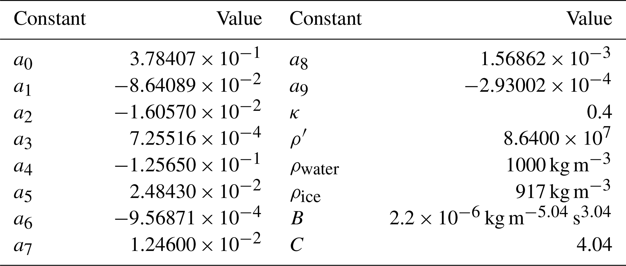
In ERA-5, snow is regarded as an additional layer on top of the soil layer and is characterised by a snow temperature T_sn with independent and prognostic thermal and mass contents. Snow melting takes place if T_sn exceeds the melting point (273.16 K), while snow sublimation is estimated with the bulk aerodynamic formula using the wind speed and specific humidity of the lowest model layer and the saturated specific humidity at T_sn (ECMWF, 2016). The bulk aerodynamic formula used in ERA-5 performed well in estimating the observed snow sublimation over the Himalayas (Stitger et al., 2018) but has not been evaluated over Antarctica. In addition, blowing snow is not accounted for in the reanalysis dataset, which is problematic as during Foehn events it is known to lower the albedo, increase surface compaction and enhance the effects of Foehn on the snowpack (e.g. Bromwich, 1989; Scarchilli et al., 2010; MacDonald et al., 2018; Datta et al., 2019; Pradhananga and Pomeroy, 2022). As a result, the terms Q_surf, D and Q_snow in Eq. (2) are estimated as detailed below, while P and M are taken directly from the reanalysis. The ERA-5-predicted surface mass anomaly, given by precipitation minus sublimation with the monthly mass accumulation over the period 1980–2001 removed, over Dronning Maud Land in East Antarctica for 2006–2017 compares well with that estimated from the measurements collected by the Gravity Recovery and Climate Experiment satellite (Gossart et al., 2019). In fact, ERA-5 is the best-performing reanalysis product out of those considered, closely following the satellite-derived estimates, with a mean absolute error of 24 Gt yr⁻¹. This justifies the use of the reanalysis' P and M data in this work. All constants are defined in Table 1.

The surface sublimation rate, Q_surf, included in the term E in Eq. (2) and following van den Broeke (1997) and Dery and Yau (2002) is parameterised as

$$\begin{array}{}\text{(3)}& Q_{\mathrm{surf}}={\mathit{\rho }}^{\prime }{\displaystyle \frac{{\mathit{\rho }}_{\mathrm{air}}\stackrel{\mathrm{‾}}{\left(w^{\prime }{q}^{\prime }\right)}}{{\mathit{\rho }}_{\mathrm{water}}}}={\mathit{\rho }}^{\prime }{\displaystyle \frac{{\mathit{\rho }}_{\mathrm{air}}\left(u_{\ast }{q}_{\ast }\right)}{{\mathit{\rho }}_{\mathrm{water}}}},\end{array}$$

with

$$\begin{array}{c}{\displaystyle }{u}_{\ast }={\displaystyle \frac{\mathit{\kappa }U}{\ln \left(\frac{z+z_{\mathrm{0}}}{z_{\mathrm{0}}}\right)}}\\ {\displaystyle }{q}_{\ast }={\displaystyle \frac{\mathit{\kappa }{q}_{\mathrm{si}}\left({\mathrm{RH}}_{\mathrm{ice}}-\mathrm{1}\right)}{\ln \left(\frac{z+z_q}{z_q}\right)}},\end{array}$$

where u_∗ is the friction velocity, q_∗ is a humidity scale, κ is the von Karman constant, U is the wind speed at height z above the surface (taken to be 10 m), z₀ is the aerodynamic roughness length, q_si is the saturation mixing ratio over ice, RH_ice is the relative humidity with respect to ice, z_q is the roughness length for moisture over snow (taken to be the same as z₀), ρ is the air density, ρ_water is the density of water and ρ^′ is a conversion factor from m s⁻¹ to mm d⁻¹. If RH_ice>1, q_∗ becomes positive and deposition to the surface is said to occur. The term $\stackrel{\mathrm{‾}}{\left(w^{\prime }{q}^{\prime }\right)}$is the turbulent moisture flux at the surface, with ${\mathit{\rho }}_{\mathrm{air}}\stackrel{\mathrm{‾}}{\left(w^{\prime }{q}^{\prime }\right)}$ giving the sublimation rate (van den Broeke, 1997). The rate of water equivalent lost to sublimation is obtained by dividing the sublimation rate by the density of water, as done by Montesi et al. (2004).

The blowing-snow sublimation rate, Q_snow, following Dery and Yau (2002), is expressed as in Eq. (4) below

$$\begin{array}{}\text{(4)}& Q_{\mathrm{snow}}={\displaystyle \frac{\begin{array}{c}{a}_{\mathrm{0}}+a_{\mathrm{1}}\mathit{\xi }+a_{\mathrm{2}}{\mathit{\xi }}^{\mathrm{2}}+a_{\mathrm{3}}{\mathit{\xi }}^{\mathrm{3}}+a_{\mathrm{4}}{U}_{\mathrm{10}}+a_{\mathrm{5}}\mathit{\xi }{U}_{\mathrm{10}}\\ +a_{\mathrm{6}}{\mathit{\xi }}^{\mathrm{2}}{U}_{\mathrm{10}}+a_{\mathrm{7}}{U}_{\mathrm{10}}^{\mathrm{2}}+a_{\mathrm{8}}\mathit{\xi }{U}_{\mathrm{10}}^{\mathrm{2}}+a_{\mathrm{9}}{U}_{\mathrm{10}}^{\mathrm{3}}\end{array}}{U^{\prime }}},\end{array}$$

with

$$\begin{array}{c}{\displaystyle }\mathit{\xi }={\displaystyle \frac{{\mathrm{RH}}_{\mathrm{ice}}-\mathrm{1}}{\mathrm{2}{\mathit{\rho }}_{\mathrm{ice}}\left[F_k\left(T\right)+F_{\mathrm{d}}\left(T\right)\right]}},\\ {\displaystyle }{U}^{\prime }={\displaystyle \frac{{\left(\mathrm{1}-\frac{U_{\mathrm{t}}}{U_{\mathrm{10}}}\right)}^{\mathrm{2.59}}}{{\left(\mathrm{1}-\frac{\mathrm{6.975}}{U_{\mathrm{10}}}\right)}^{\mathrm{2.59}}}},\\ {\displaystyle }{U}_{\mathrm{t}}=\mathrm{6.975}+\mathrm{0.0033}{\left(T_{\mathrm{2}\mathrm{m}}+\mathrm{27.27}\right)}^{\mathrm{2}},\end{array}$$

where ξ is a thermodynamic term, U₁₀ is the 10 m wind speed, U^′ is a non-dimensional factor that removes the dependence on the saltation mixing ratio, U_t is the threshold for initiation of blowing snow, T_2 m is the 2 m temperature, ρ_ice is the density of ice, and F_k(T) and F_d(T) are the conductivity and diffusion terms associated with sublimation, both of these latter terms are temperature dependent and extracted from Rogers and Yau (1989). The values of the constants a₀–a₉ are obtained for a site in the Canadian Arctic, as detailed in Dery and Yau (2002). The lack of in situ measurements at PIG prevents us from assessing whether they are optimal for this region, which is a caveat on the estimation of Q_snow. While negative values of Q_surf indicate sublimation and positive values denote deposition, the opposite is true for Q_snow, with positive values implying sublimation of blowing snow is taking place.

The snow transport rate, Q_t, is a vector quantity whose magnitude is given by

$$\begin{array}{}\text{(5)}& {\mathit{Q}}_{\mathrm{t}}=B{U}_{\mathrm{10}}^C,\end{array}$$

with the direction obtained by projecting it onto the 10 m horizontal wind vector. Constants B and C are derived from measurements collected in the Canadian Prairies (Dery and Yau, 2002), and an assumption is made that they are reasonable for PIG. The divergence term D in Eq. (2) is then obtained by

$$\begin{array}{}\text{(6)}& D={\displaystyle \frac{{\mathit{\rho }}^{\prime }}{{\mathit{\rho }}_{\mathrm{water}}}}\mathrm{\nabla }\cdot {\mathit{Q}}_{\mathrm{t}}.\end{array}$$

Table 1 Constants used in the surface mass balance.

3 Foehn events at PIG and impacts on ice

The statistics of Foehn events at PIG are summarised in Fig. 2. Foehn is more frequent in the austral winter season, in particular from June to October, and less common in the summer but with a considerable spread in all months (Fig. 2a). The annual cycle in the duration of Foehn events is less pronounced, with monthly mean values in the range 5 to 9 h, with August featuring both the highest number (∼ 123) and longest (∼ 9 h) Foehn episodes. At the Antarctic Peninsula, Foehn occurrence peaks in the transition seasons (Wiesenekker et al., 2018; Laffin et al., 2021), whereas at the McMurdo Dry Valleys located next to the Ross Sea it is more frequent in winter (Speirs et al., 2013). As Foehn events are driven by large-scale pressure gradients, the difference in the timing of the peaks is likely a result of the variability in the position of the baroclinic systems. In particular, as noted by Simmonds et al. (2003), the cyclonic activity in the Ross Sea, northern Antarctic Peninsula and around PIG is maximised in winter, whereas in the central Antarctic Peninsula it is highest in the summer. Consistent with this, in the Amundsen and Bellingshausen seas there is a pronounced equatorward shift in the mid-latitude storm track in the summer months (Dias da Silva et al., 2021), which is in line with the higher occurrence of Foehn at PIG in the colder months. The Amundsen Sea Low (ASL), a semi-permanent low-pressure centre in the Amundsen and Bellingshausen seas (60–75^∘ S and 170–290^∘ E) that exhibits the largest geopotential height variability in the Southern Hemisphere, is likely to play a major role in the occurrence of Foehn at PIG (Mclennan and Lenaerts, 2021). Meridionally, it is at its most poleward location in late winter and is shifted further equatorwards in the summer, while longitudinally it is the closest to PIG in the summer months (Raphael et al., 2016). As Foehn is more likely when the ASL is just to the north of PIG, with its clockwise circulation encouraging Foehn effects in the region, as noted in Sect. 4, the intricate annual cycle of the ASL may explain the highest Foehn occurrence in late winter and why it still takes place in the summer months. In the area around PIG, there are on average 3.0 Foehn days in the month of August (123 occurrences over the 41-year period 1980–2020) lasting roughly 7.9 h each, whereas in January there are 0.37 Foehn days per month that typically last for about 5.1 h. Wiesenekker et al. (2018) reported an average of 1.3 to 5.8 Foehn events per month in the Antarctic Peninsula over 1979–2016, with roughly 70 %–80 % of the events in December 2014–December 2016 lasting less than a day. These figures are higher than those at PIG shown in Fig. 2a, which is due to the fact that the Antarctic Peninsula is more exposed to the mid-latitude storm track, with the higher terrain on its western side promoting Foehn effects.

Figure 2b gives the area-averaged air temperature and sensible heat flux for the Foehn events, with the air temperature, sensible heat flux and RH anomalies during Foehn episodes plotted in Fig. 2c. The sensible heat flux is positive, and hence it is directed downwards towards the surface, with monthly mean values in the range 18 to 42 W m⁻² and higher values in the winter months. This is in line with Laffin et al. (2021) and with the fact that the sensible heat flux around Antarctica is maximised in the colder months when the surface to air temperature gradient is the highest, owing to the sharp thermal inversions that develop at this time of the year (Reijmer et al., 1999). The magnitude of the fluxes is comparable to that modelled over the Antarctic Peninsula (e.g. Elvidge et al., 2016) and at Joyce Glacier in the McMurdo Dry Valleys (Hofsteenge et al., 2022). The air temperature during Foehn events at PIG is below freezing, ranging from −7 in January to −22 ^∘C in August. However, melting and sublimation can still occur, in particular when accounting for the large variability, which is maximised in the summer (e.g. Ghiz et al., 2021). Figure 2c shows that Foehn effects lead to generally warmer (air temperatures anomalies typically of +0–7 ^∘C) and drier (RH anomalies in the range −8 % to −11 %) weather conditions accompanied by a downward sensible heat flux (anomalies of +14–21 W m⁻²).

Figure 2d gives the trends in the number of Foehn days and in the duration of Foehn events for 1980–2020, both of which are not statistically significant. When the analysis is extended to individual seasons, only one statistically significant trend is found, i.e. that of the duration for the autumn season, with a slope of about −0.002 d yr⁻¹ (not shown). Studies of trends of Foehn occurrence in Antarctica also reported statistically non-significant slopes, in particular over the two major studied regions of the McMurdo Dry Valleys (e.g. Speirs et al., 2013) and the Antarctic Peninsula (e.g. Laffin et al., 2021). Figure 2d also shows considerable inter-annual variability in both the number and duration of Foehn days. The major peaks taking place mostly in La Niña (1984, 1985, 1999, 2010) or neutral (1981, 1993, 1996, 1999, 2003, 2008, 2013) years, while the minima in 1982, 1986, 1997 and 2015 coincide with El Niño years (Lestari and Koh, 2016; Zhang et al., 2022). In La Niña conditions, the ASL is more active than normal (Raphael et al., 2016), which may promote the occurrence of Foehn, while in El Niño episodes the presence of a ridge over the Amundsen and Bellingshausen seas (Yuan, 2004) may discourage Foehn effects at PIG. A discussion of the large-scale patterns that favour Foehn occurrence at PIG is given in Sect. 4.

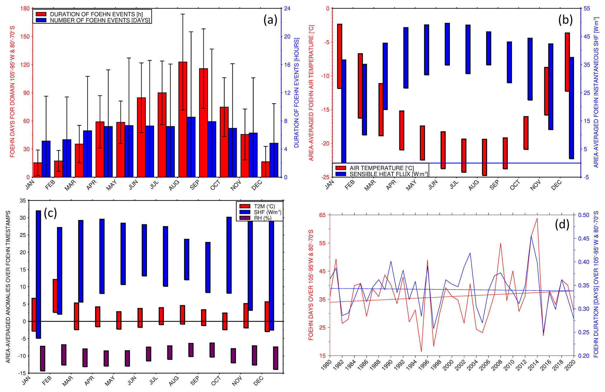
Figure 2 Climatology and trends of Foehn events. (a) Monthly mean (histogram bars) and standard deviation (error bars) of Foehn days (orange; left axis) and duration of Foehn events (hours; blue; right axis) for the period 1980–2020 and for the domain 80–70^∘ S and 95–105^∘ W. (b) Box plot of the area-averaged air temperature (^∘C; orange; left axis) and instantaneous sensible heat flux (W m⁻²; blue; right axis; positive if downwards towards the surface) giving the mean ± 1σ for Foehn episodes. Panel (c) is the same as panel (b) but for the air temperature (^∘C; orange), instantaneous sensible heat flux (W m⁻²; blue) and relative humidity (%; purple) anomalies during Foehn timestamps. (d) Trend in Foehn days (left; red) and in the duration of Foehn events (right; blue) for 1980–2020. The slopes of the Foehn days and duration are 0.101024 and −0.0001 d yr⁻¹ with a statistical significance of 55 % and 18 %, respectively.

A quantification of the potential for surface melting and sublimation is presented in Fig. 3. The “melt potential” index (MPI) is defined following Orr et al. (2022) using the daily maximum air temperature for 1980–2020 for both the full year and extended summer season (November to February, NDJF). At each grid point, the MPI intensity is given by the difference between the 95th percentile of the daily maximum air temperature distribution for the Foehn and no-Foehn days and the melt threshold of 273.15 K, while the MPI frequency is the percentage of values higher than the threshold. The “sublimation potential” index (SPI) is defined in the same way but using the 95th percentile of the daily maximum of the hourly surface sublimation given by Eq. (3) and a threshold of zero, while its frequency expresses the percentage of the Foehn and no-Foehn days in the 1980–2020 period when there is sublimation for at least 1 h d⁻¹ at the site. Here, the difference between Foehn and no-Foehn timestamps is plotted for both indices to give insight into the effects of Foehn in surface melting and sublimation.

Surface melting is less common at PIG during Foehn events, with a MPI intensity and frequency reductions of about −1.3 K and −3 %, respectively, with comparable values in NDJF (−0.9 K and −6 %). As noted in Elvidge et al. (2020), during Foehn events the downward sensible heat flux in response to the warmer near-surface air is largely offset by the upward latent heat flux that arises from the drier conditions. The surface energy balance is then controlled by the radiation (mostly long wave in the colder months) and ground heat fluxes, which may make it harder for the snowpack to melt compared to no-Foehn days. Surface melting is confined to lower elevations where the temperature is higher. Here, there is also increasing exposure to the warmer and more moist maritime air masses compared to the high terrain inland. The fact that surface melting is more frequent in the coastal areas adjacent to the Southern Ocean in Foehn episodes may be attributed both to the increased adiabatic compression of the winds as they descend towards the low elevations and the likely presence of a low-pressure system north of the site during the Foehn events, as will be discussed in Sect. 4. When all days (Foehn and no-Foehn days) in 1980–2020 are considered, the MPI intensity and frequency at PIG for the full year are −0.27 K and 4 %, respectively, and +0.87 K and 10 % for NDJF, respectively (not shown). Orr et al. (2022) used higher-spatial-resolution (∼ 12 km) modelling products over December–February 1979–2019 and for the entirety of Antarctica to obtain values at PIG of 1.3–1.7 K and 23.7 %–23.8 %. The MPI intensity and frequency difference between Foehn and no-Foehn days given in Fig. 3a–b stress the role of Foehn in discouraging surface melting at and around the glacier. Figure 3c–d are the same as Fig. 3a–b but for the SPI. The seasonal variability is much reduced compared to that of the MPI, with an intensity difference between Foehn and no-Foehn days of +1.8 mm w.e. d⁻¹ for the full year and +1.6 mm w.e. d⁻¹ for NDJF and a rather small change in frequency (<0.3 %). When all days are taken into account, the intensity magnitudes are of about 3.34 and 3.39 mm w.e. d⁻¹, respectively, and the frequency of occurrence is around 100 % (not shown). The fact that the frequency is very high indicates that the daily maximum in the surface sublimation is positive nearly all the time at PIG, suggesting that there is at least 1 h of sublimation every day of the year for the 41-year period at the site. This also explains why there is hardly any change in frequency between Foehn and no-Foehn days. The SPI intensity, on the other hand, is roughly 50 % larger during Fohn episodes, highlighting the role of Foehn effects in the surface sublimation. It is interesting to note that even though the near-surface wind in the region is stronger in the colder months, the effects of Foehn on the 10 m wind in NDJF are largely similar to those in the full year (see Fig. 3c–d). The convergence of the near-surface wind in the PIG basin and the lower heights and consequently higher temperatures explains the maximum in surface sublimation in the region seen in Fig. 3c–d.

In order to explore the contribution of Foehn to the surface mass balance, Fig. 4a–f show the composite difference of the terms in Eq. (2) between Foehn and no-Foehn timestamps for 1980–2020. The Foehn minus no-Foehn values of the rate of accumulation or storage of snow at the surface (S), precipitation (snowfall) rate (P), surface melt and runoff rate (M), surface sublimation rate (Q_surf), blowing-snow sublimation rate (Q_snow), and blowing-snow divergence rate (D) at the closest grid point to PIG are $S\sim -\mathrm{1.41}$, $P\sim -\mathrm{0.35}$, $M\sim -\mathrm{0.01}$, $Q_{\mathrm{surf}}\sim -\mathrm{1.43}$, Q_snow∼0, and $D\sim -\mathrm{0.36}$ mm w.e. d⁻¹, respectively. This indicates that (i) surface sublimation plays the dominant role in the surface mass balance during Foehn events (note that negative values of the surface sublimation rate, Q_surf, and positive values of the blowing-snow sublimation rate, Q_snow, indicate sublimation); (ii) the sum of the two blowing-snow terms, Q_snow and D, has a magnitude comparable to that of the precipitation and snowfall, P, roughly 25 % smaller than that of the surface evaporation, but with the opposite sign in Eq. (2), reflecting a lack of snowfall during Foehn episodes due to the drier conditions while the convergence of blowing snow at the glacier basin adds to the surface mass; (iii) snow melting, M, makes a negligible contribution to the surface mass balance, being roughly 3 orders of magnitude smaller than the surface sublimation. The lack of in situ measurements at PIG precludes an evaluation of the above estimates. In any case, the fact that the blowing-snow terms can play an important role in the surface mass balance has been highlighted by other authors: for example, Scarchilli et al. (2010) reported that at Terra Nova Bay in the Ross Sea, where wind speeds can exceed 40 m s⁻¹ (Fonseca et al., 2023), blowing-snow sublimation and snow transport remove (mainly in the atmosphere) up to 50 % of the precipitation in the coastal and slope convergence areas. The authors found that the cumulative snow transportation is roughly 4 orders of magnitude larger than the snow precipitation at that site. At PIG, winds increase by 10 m s⁻¹ during Foehn days compared to no Foehn days (Fig. 4g), which favours a large contribution of blowing-snow sublimation and blowing-snow divergence to the surface mass balance.

The surface sublimation rate (Fig. 4c) is considerable, with the values at PIG comparable to the maximum rates at a site in northern Victoria Land during November 2018 (Ponti et al., 2021), but it is roughly an order of magnitude smaller than that due to melting resulting from ice dynamics around Antarctica, including at PIG (Holland et al., 2007; Rintoul et al., 2016; Feldmann et al., 2019). Surface melting is negligible and confined to the coastal regions further north (Fig. 4d). As noted by Scarchilli et al. (2010) and in line with our findings (Fig. 4e–f), blowing snow plays an important role in the surface mass balance during strong wind (here Foehn) episodes. The magnitude of the total blowing-snow sublimation and transport reported in that study, which are measured at the Terra Nova Bay in the Ross Sea, are larger than those estimated here at PIG. This is consistent with the fact that katabatic wind events at Terra Nova Bay can be quite strong, being associated with much higher wind speeds than those during the Foehn events discussed here (Aulicino et al., 2018). Blowing-snow sublimation (Fig. 4e) peaks just south and east of the glacier, with values in the range 0.5–0.75 mm w.e. d⁻¹, where the wind speed exceeds the threshold for blowing-snow sublimation; see Eq. (4). The convergence of the blowing-snow transport rate from the east and southeast of PIG leads to the negative divergence at the basin (Fig. 4f). The negative values in the snowfall rate plot to the south and north of PIG (Fig. 4b) reflect the reduced precipitation in association with Foehn events. The changes in the storage term between Foehn and no-Foehn timestamps (Fig. 4a) are comparable to the modelled surface mass balance in the region (Donat-Magnin et al., 2021), suggesting that Foehn events are a major contributor to it. Figure 4g–h give the differences in the 10 m wind speed and sensible heat flux. During Foehn episodes, there is a strengthening of the near-surface wind by 5–10 m s⁻¹ with it converging into PIG. The sensible heat flux increases by about 30–40 W m⁻², in line with the area-averaged values in Fig. 2b. While in other regions of Antarctica, such as the Antarctic Peninsula, Foehn plays an active role in snow melting (Laffin et al., 2021), at PIG it seems to trigger mostly sublimation.

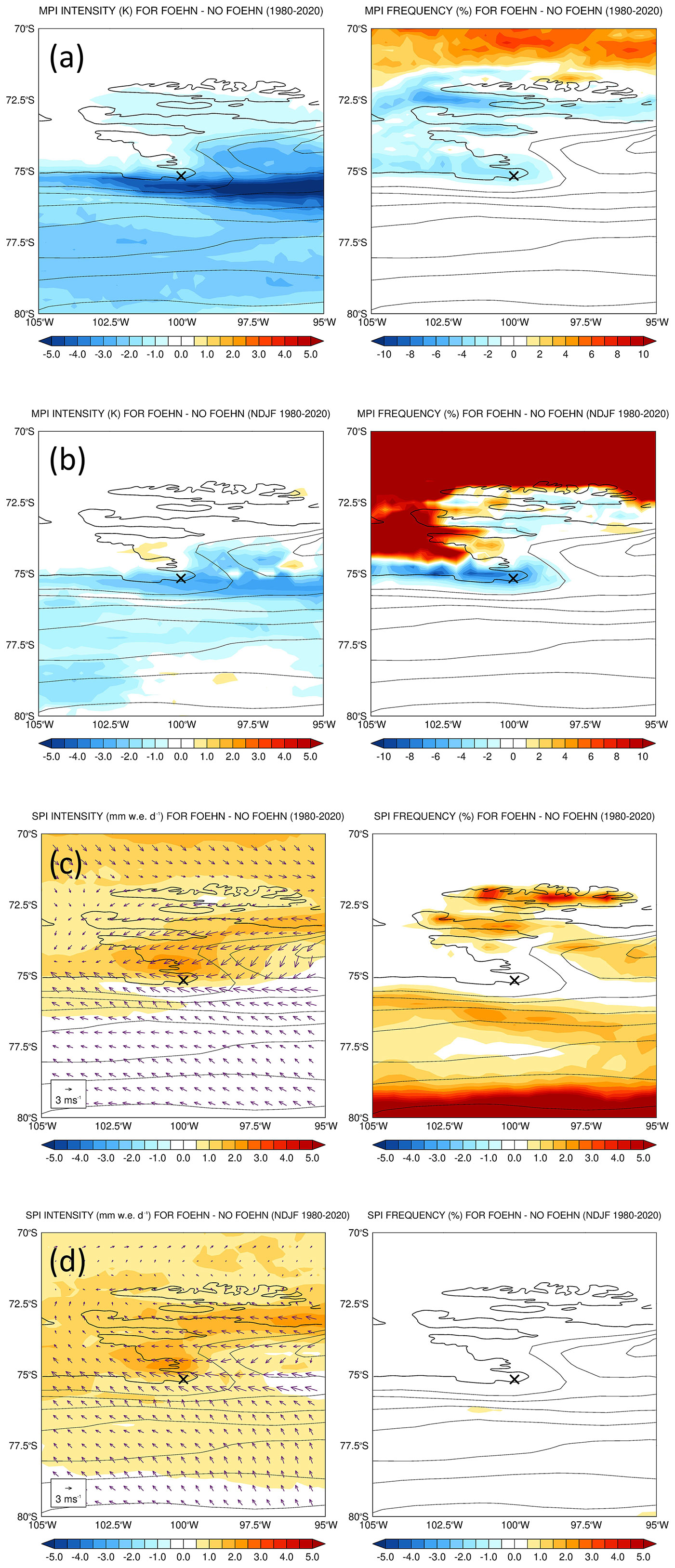
Figure 3 Melt and sublimation potential indices. (a) Melt potential index (MPI) intensity (K; left) and frequency (%; right), defined following Orr et al. (2022), for the difference between Foehn and no-Foehn timestamps for 1980–2020. The thin black lines are 250 m orography contours and the land–sea mask is represented by the thick black line. The cross gives PIG location (75^∘10^′ S, 100^∘ W). Panel (b) is the same as (a) but for November–February (NDJF) only. Panels (c)–(d) are the same as (a)–(b) but for the sublimation potential index (SPI), with the intensity given in millimetres of water equivalent per day (mm w.e. d⁻¹). The averaged 10 m horizontal wind vectors are drawn as arrows in the left panels of (c)–(d) for the respective period.

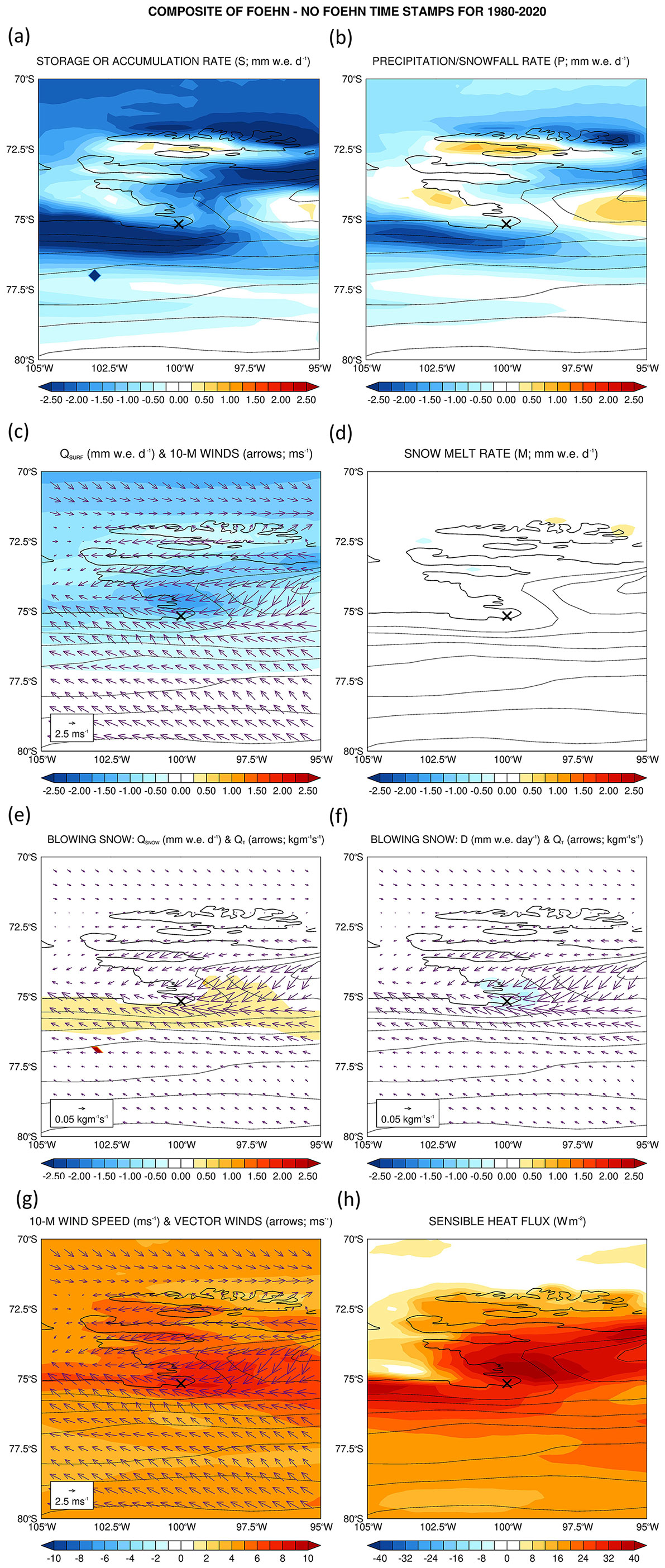
Figure 4 Composite difference between Foehn and no-Foehn timestamps for 1980–2020. (a) Storage or accumulation rate of snow at the surface (S in Eq. (2); mm w.e. d⁻¹), (b) precipitation and snowfall rate (P; mm w.e. d⁻¹), (c) surface sublimation rate (Q_surf; mm w.e. d⁻¹; positive values indicate deposition to the surface, and negative values indicate sublimation), (d) snowmelt rate (M; mm w.e. d⁻¹; positive values indicate melting), (e) blowing-snow sublimation rate (Q_snow; mm w.e. d⁻¹; positive values indicate sublimation), (f) blowing-snow divergence rate (D; mm w.e. d⁻¹), (g) 10 m wind speed (shading; m s⁻¹) and (h) instantaneous surface sensible heat flux (W m⁻², positive if downwards towards the surface). The arrows in (c) and (g) give the 10 m horizontal wind vectors (m s⁻¹), while in (e) and (f) they show the blowing-snow transport rate (Q_t; kg m⁻¹ s⁻¹).

4 Large-scale circulation favourable for Foehn occurrence

Foehn events are driven by large-scale pressure gradients, so it is of interest to investigate the patterns in the atmospheric circulation that promote their occurrence around PIG. The k-means clustering technique (Steinley, 2006) is applied to the daily 200 and 850 hPa geopotential height and wind anomalies and to the sea level pressure and 10 m wind anomalies for the Foehn days identified in 2000–2020. However, to exclude localised events, only days when Foehn occurred in at least 10 % of the 70–80^∘ S and 105–95^∘ W region are considered, leaving 1181 d for the analysis. Different numbers of clusters from one to five are tested, and the optimal number, as determined by a silhouette analysis (Rousseeux, 1987), is found to be two (not shown). Cluster 1 (Fig. 5a–b), which features the negative phase of the Antarctic oscillation (AAO; Gong and Wang, 1999), accounts for ∼ 58 % of the total Foehn events. Cluster 2 (Fig. 5c–d), which projects onto the positive phase of the Southern Annular Mode (SAM; Marshall, 2003), an index that gives an indication of the strength and latitudinal position of the westerlies in the Southern Hemisphere, accounts for ∼ 42 % of the 1181 Foehn episodes. The clusters' annual cycle is given in Fig. 5e. For computational reasons the cluster analysis was not extended to 1980–2020. In any case, the findings are unlikely to change should the technique be applied to the 41-year period, with the AAO and SAM most certainly the dominant modes.

The first cluster (Fig. 5a) comprises a wavenumber, no. 1, with an equatorward shift in the mid-latitude storm track as evidenced by the high pressure over Antarctica and a nearly circumglobal low pressure equatorwards. It corresponds to the negative phase of the AAO, with the easterly to northeasterly winds around PIG promoting the occurrence of Foehn. The air mass comes from the Weddell sector and moves over the Ellsworth Land before flowing down the length of PIG drainage basin (Fig. 5b). The wavenumber no. 1 is maintained by both low-latitude forcing (Quintanar and Mechoso 1995a and b) and the high topography of Antarctica (Hoskins and Karoly, 1981). As noted by Pohl et al. (2010), the AAO has a strong correlation with the El Niño-Southern–Oscillation (ENSO), with El Niño events favouring its negative phase. This mode dominates in the colder months from May to August (Fig. 5e) when the ASL is displaced westwards (Raphael et al., 2016), and hence the SAM has a smaller impact on the weather conditions at PIG.

The second cluster (Fig. 5c) projects onto the positive phase of the SAM in which the storm track is shifted poleward and the ASL is significantly deeper (Fogt and Marshall, 2020; Zheng and Li, 2022). Mclennan and Lenaerts (2021) found that the ASL modulates the total annual snowfall at the Thwaites Glacier adjacent to PIG (Fig. 1a). This cluster shows the winds descending the slopes immediately to the east of the Pine Island ice shelf. The air mass comes from the Pacific Ocean and flows over the high terrain and coastal mountains directly to the northeast of PIG before descending downslope into the glacier basin (Fig. 5d). The cyclonic (clockwise) circulation associated with the ASL and its interaction with the high terrain to the east of PIG lead to Foehn conditions around the glacier. The second cluster features a wavenumber no. 3 across the Southern Hemisphere (Goyal et al., 2021). Simulations for the more extreme climate change scenarios suggest a tendency for more positive SAM in a warming world, accompanied by a poleward shift in the ASL in summer and autumn and an eastward shift in autumn and winter (e.g. Hosking et al., 2016; Gao et al., 2021). Such an occurrence may increase the frequency and perhaps strength of Foehn events at PIG.

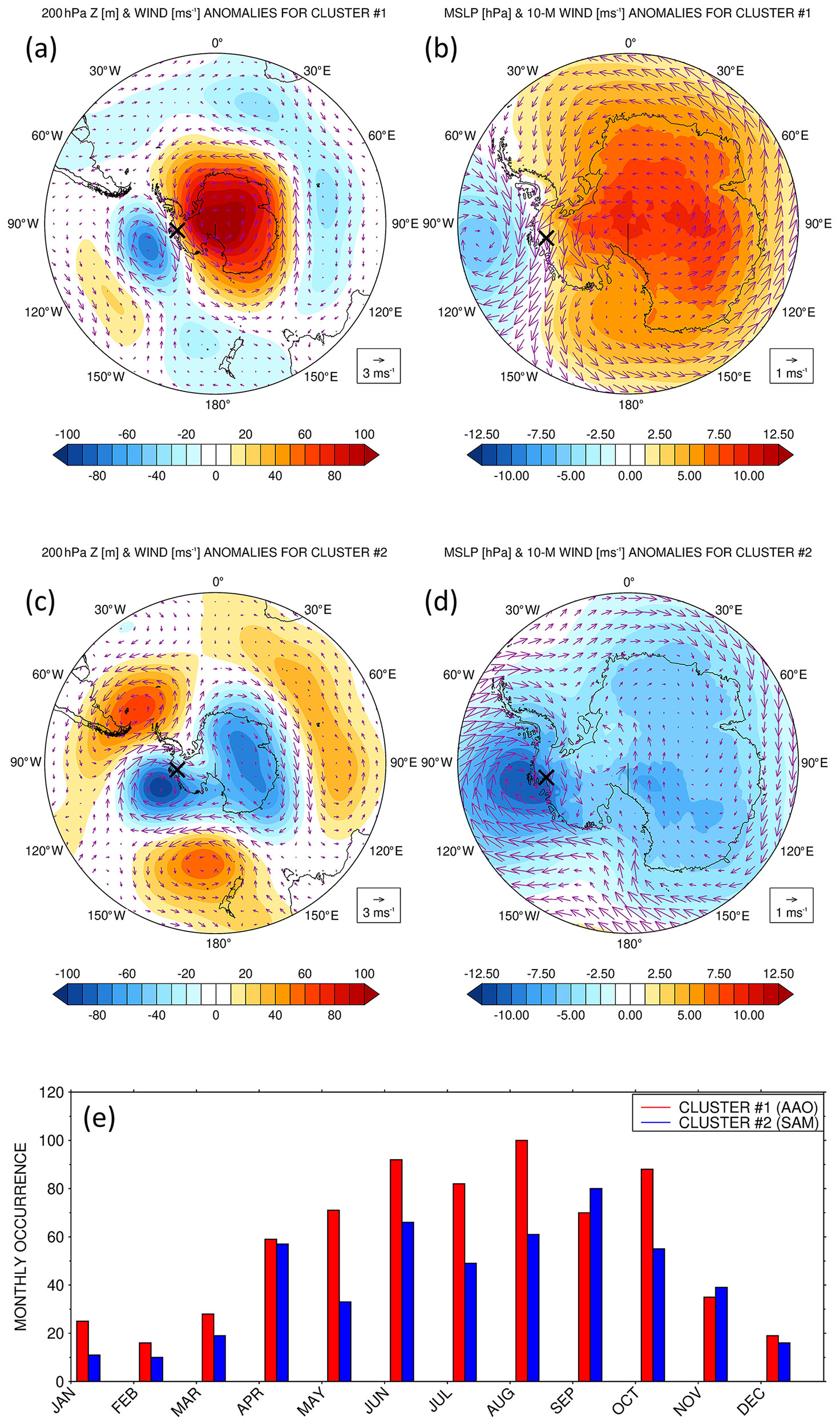
Figure 5 Large-scale conditions promoting Foehn events. The (a) 200 hPa geopotential height anomalies (shading; m) and wind vectors (arrows; m s⁻¹) and (b) mean sea level pressure (shading; hPa) and 10 m wind vectors (arrows; m s⁻¹) for cluster 1 of a k-means clustering technique applied to the daily mean fields of 1181 Foehn days at PIG in 2000–2020. The cross gives the approximate location of PIG (100^∘ W, 75^∘10^′ S). Panels (c)–(d) are the same as (a)–(b) but for cluster 2. The monthly occurrence of each cluster is given in panel (e).

5 Illustrative case study: November 2011

The effects of Foehn at PIG are discussed for an event in November 2011. Figure 6 summarises the large-scale environment that promoted the occurrence of Foehn, while Fig. 7 presents a time series of spatially averaged meteorological variables that allows for a quantification of the Foehn effects.

The ASL was particularly deep on 10–11 November 2011, with the 500 hPa geopotential height anomalies more than 1.5σ below the 1979–2020 mean (Fig. 6a–b). An atmospheric river associated with an elongated and narrow band of high moisture content and integrated vapour transport (IVT) values in the top 10 % of the climatological distribution extended from the Southern Hemisphere mid-latitudes into West Antarctica and PIG, transported by the clockwise circulation of the ASL. As the ASL edged closer to the Antarctic Peninsula on 11 November (Fig. 6b), the more moist air, now over the Weddell Sea, penetrated further inland reaching PIG and the surrounding region from the east (after flowing over the ice divide that separates the Weddell Sea and Ronne Ice Shelf from PIG and the Amundsen Sea region). As a result, the IVT at PIG more than doubled from about 27.5 kg m⁻¹ s⁻¹ on 10 November to around 65 kg m⁻¹ s⁻¹ on 11 November, with the total column water vapour increasing to just under 4 kg m⁻² (Fig. 7a). The Foehn effect in this event corresponds to that of cluster 1 (Fig. 4a), the more indirect pathway from the Weddell Sea, as opposed to Foehn events triggered by Pacific warm air intrusions (cluster 2, Fig. 4b).

As seen in Fig. 6c–d, the air mass accelerated downslope as it descended the mountains towards coastal West Antarctica, with 10 m wind speeds higher than 20 m s⁻¹ and in the top 10 % of the climatological distribution over a vast region including PIG (locally in the top 1 % just to the northwest and southeast of PIG) and downward sensible heat fluxes in excess of 75 W m⁻² at PIG (the negative, or upward pointing, fluxes around 75^∘ S and 110^∘ W are associated with a sea-ice-free area). These tendencies are seen in the area-averaged time series (Fig. 7c), with the negative (upward) latent heat flux indicating sublimation peaking on 11 November (Fig. 7f). In fact, the phase of the latent heat flux matches that of the surface sublimation given in Fig. 7f. The opposite sign of the sensible and latent heat fluxes, which roughly offset each other, is expected during Foehn events (Elvidge et al., 2020), as the positive latent heat flux that arises due to sublimation is opposed by the downward sensible heat flux due to the higher temperature in the air than at the surface. The surface mass balance is essentially controlled by the surface and blowing-snow sublimation, with the precipitation and snowfall and the divergence terms playing a secondary role and snow melting being zero throughout the full period (Fig. 7f). The estimated maximum sublimation rate is seen at the end of 10 November and has a magnitude of ∼ 0.13 mm w.e. h⁻¹, comparable to the ice loss due to ocean dynamics (e.g. Holland et al., 2007; Rintoul et al., 2016; Feldmann et al., 2019), although not in a sustainable way. The ERA-5 snow depth, which accounts only for sublimation and changes in snow density (snowmelt is not simulated by ERA-5 during this event, Fig. 7f), shows a steady decrease starting on 4 November and a faster drop from 11–13 November (not shown). The reanalysis snow depth during this period is around 9.21 m w.e., within the range of that observed during field campaigns discussed in Konrad et al. (2019). Besides sublimation, melting was detected in the Moderate Resolution Imaging Spectroradiometer (MODIS; Kaufman et al., 1997) satellite imagery, reaching a maximum on 12 November (Fig. 7g). The melting area at times exceeded ∼ 100 km² or roughly 2 % of the central trunk of the glacier (Wingham et al., 2009). The fact that ERA-5 does not simulate the observed melting can be attributed to the way snow melting is parameterised in the model used to generate the reanalysis dataset, only taking place if the temperature of the snow layer exceeds the melting point (ECMWF, 2016), with ERA-5 exhibiting a cold bias over the high terrain in Antarctica (e.g. Gonzalez et al., 2021). The observed melting area is also much smaller than ERA-5's spatial resolution (∼ 27 km × 27 km). Further insight into the surface melt can be gained by running a surface balance model at high spatial resolution that can be driven by ERA-5 data. This will be left for future work.

In Fig. 7d–e, the net short-wave, long-wave and radiation fluxes from the reanalysis data are compared with those estimated from satellite data, as given by the Clouds and Earth's Radiant Energy System (CERES) SYN1deg dataset (Doelling et al., 2013, 2016). ERA-5 under-predicts the net short-wave radiation flux during the day by up to a factor of 2.5 and the net long-wave radiation flux at night by up to 25 W m⁻². These differences are consistent with those reported by Ghiz et al. (2021), who attributed the lower short-wave fluxes in ERA-5 compared to CERES to differences in the cloud properties, with the reanalysis fluxes being more consistent with those measured in situ at a site in the West Antarctic Ice Sheet than those of CERES. On the other hand, CERES partially corrects the tendency of ERA-5 to under-predict the net long-wave radiation flux over Antarctica, in particular in clear-sky conditions (Silber et al., 2019). During the November Foehn event, the area-averaged surface energy flux, F_net, is positive (Fig. 7e), as the positive sensible heat flux offsets the negative latent heat flux (Fig. 7c), and the surface net short-wave radiation flux overwhelms the negative net long-wave flux (Fig. 7d). This indicates an excess of energy towards the surface, leading to snowmelt and evaporation. The 3–5 ^∘C increase in air temperature (Fig. 7b) with respect to the previous non-Foehn days, present in both the reanalysis and weather station data, is comparable to that seen during a Foehn event at the Ross Ice Shelf in January 2016 (Zou et al., 2019). Note that the ERA-5 values are area-averaged values over the red box in Fig. 1a, and hence the fields are likely larger in local areas.

The Foehn event can also be seen in the Hovmöller plots in Fig. 6e. The wind direction shifts from northeast to southeast on 8–9 November 2011 around PIG as the ASL moves closer to the Antarctic Peninsula. This is accompanied by an increase in the sensible heat flux, with a latitudinally averaged value exceeding 50 W m⁻² that corresponds to an anomaly of about 40 W m⁻². The fact that the peak in wind speed takes place at ∼ 90^∘ W but that in the heat fluxes is at around 100–110^∘ W is consistent with the warming of the air mass as it descends the slopes of the mountains over West Antarctica. The drying of the atmosphere in association with the Foehn effects is also present, with the RH dropping below 70 % during the event. The sensible heat flux shows a clear diurnal cycle, peaking around 05:00–06:00 UTC, which is roughly 00:00 LT (local time) for a longitude of ∼ 100^∘ W, and this is out-of-phase with the surface radiation fluxes (Fig. 7c–e). This mismatch is also seen on other days and may be attributed to the effects of Foehn, clouds and moisture on the heat fluxes. Weaker Foehn events, with peak wind speeds roughly half of speeds on 9–11 November but with similar values of RH, took place earlier in the month on 3–4 November 2011.

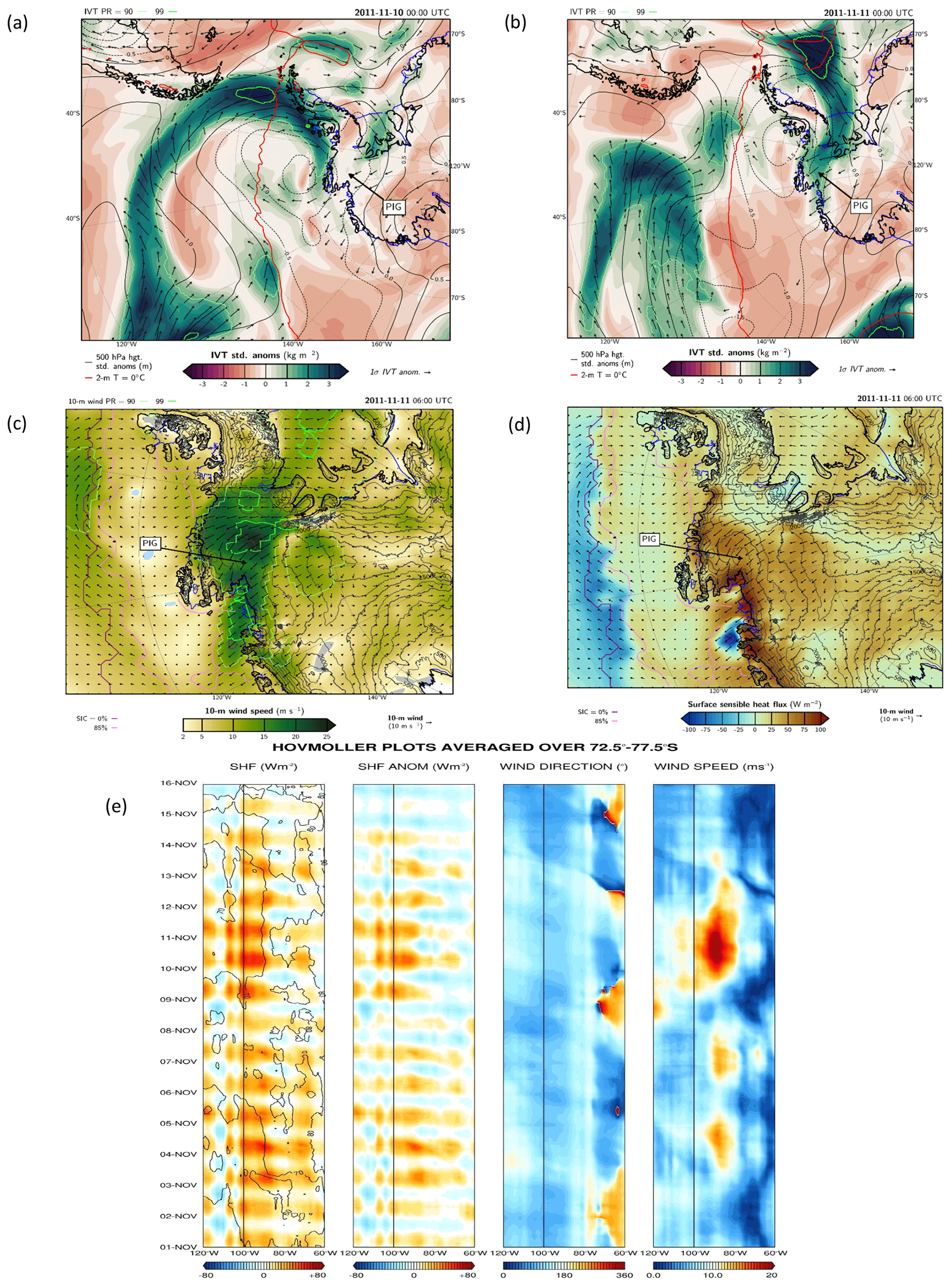
Figure 6 November 2011 Foehn events. Integrated water vapour transport (IVT; kg m⁻²; shading) standardised anomalies with respect to ERA-5's 1979–2020 monthly climatology, where the vectors give a 1 standard deviation anomaly and are only plotted if the IVT standardised anomalies exceed 1, and 500 hPa geopotential height standardised anomalies (solid contours) on (a) 10 November and (b) 11 November 2011 at 00:00 UTC. The thin and thick green lines denote the 90th and 99th IVT percentiles, respectively; the yellow star gives the location of the Evans Knoll weather station (−74.85^∘ S; −100.404^∘ W); and the solid red line is the 0 ^∘C 2 m temperature isotherm. (c) The 10 m wind speed (shading; m s⁻¹), with the 90th and 99th percentiles denoted by the solid thin and thick green lines, respectively, and 10 m winds (vectors; m s⁻¹) on 11 November 2011 at 06:00 UTC. The grey lines are orographic contours drawn and labelled every 500 m, and the dark solid purple and pink lines highlight regions where the sea ice concentration is equal to 0 % and 85 %, respectively. Panel (d) is the same as (c) but with the shading giving the sensible heat flux (shading; W m⁻²; positive if downwards towards the surface). The anomalies and percentile ranks for the IVT, 10 m horizontal winds, 500 hPa geopotential height and 2 m temperature are calculated from the distribution of all 3 h values within ±15 Julian days from the given date during the 1979–2020 period and at a given grid point. (e) Hovmöller plot of sensible heat flux (shading; W m⁻²) and relative humidity (contours, every 10 %), sensible heat flux anomalies with respect to the 1979–2021 climatology (W m⁻²), and 10 m wind direction (^∘) and speed (m s⁻¹) for 1–15 November 2011. The fields are averaged over 72.5–77.5^∘ S and are plotted for the region 120–60^∘ W. All colour bars are linear, with only the lowest, median and highest values shown. The vertical black line indicates the approximate longitude of PIG (100^∘ W).

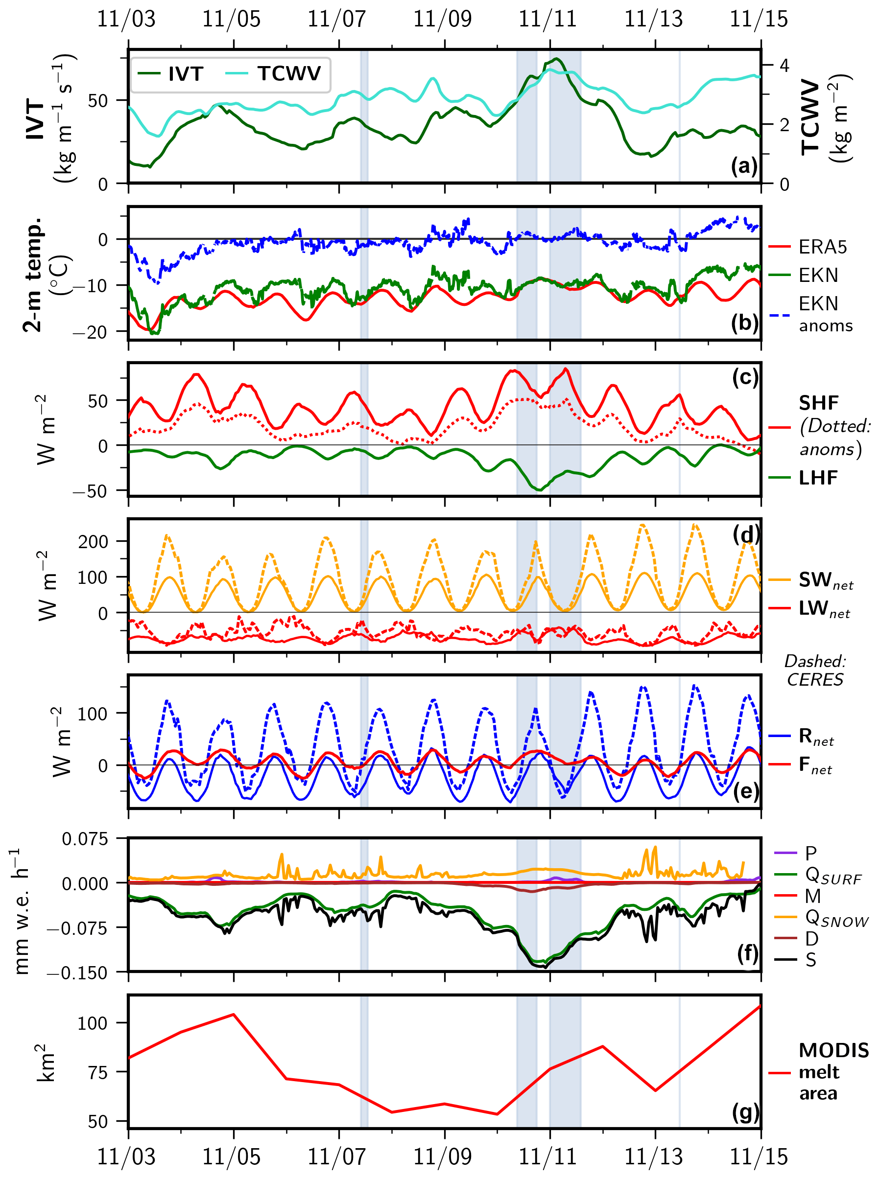
Figure 7 Impacts of Foehn winds on ice. Time series of 1-hourly ERA-5 variables averaged over PIG (red box in Fig. 1a) from 3 to 14 November 2011: (a) integrated water vapour transport (IVT; light green; kg m⁻¹ s⁻¹) and total column water vapour (TCWV; dark green; kg m⁻²); (b) 10 min observed 2 m temperature (green; ^∘C) at the Evans Knoll weather station (−74.85^∘ S, −100.404^∘ W; 188 m a.s.l.), where the anomalies with respect to the 2011–2015 hourly climatology are given by the dashed blue line, and area-averaged ERA-5 2 m temperature (red; ^∘C); (c) ERA-5 sensible heat flux (SHF; red; W m⁻²) and latent heat flux (LHF; orange; W m⁻²); (d) net short-wave radiation (SW_net; orange; W m⁻²) and long-wave radiation (LW_net; red; W m⁻²) flux at the surface; (e) net radiation (R_net; blue; W m⁻²) and total energy flux ($F_{\mathrm{net}}=\mathrm{SHF}+\mathrm{LHF}+R_{\mathrm{net}}$; red; W m⁻²) at the surface; and (f) individual components of the surface mass balance (Eq. 2), expressed in mm w.e. h⁻¹. The S, P, M, Q_surf, Q_snow and D terms are given by the black, purple, red, green, orange and brown lines, respectively. (g) Daily total surface area (km²) of melt ponds observed from MODIS imagery. In panel (c), the SHF anomalies, calculated as the difference from the domain-averaged 1979–2020 November hourly monthly mean, are also plotted. In (d)–(e), the net radiative variables from CERES averaged over the same domain are plotted as dashed lines for comparison. Times when Foehn occurred are shaded in blue.

6 Conclusions

Pine Island Glacier (PIG), located in West Antarctica around 75^∘ S and 100^∘ W between the Antarctic Peninsula to the east and the Ross Ice Shelf to the west, has been losing ice mass at an accelerated rate over the last 2 decades. While the vast majority of the studies on ice loss at PIG focus on ocean dynamics (e.g. Stanton et al., 2013; Favier et al., 2014), atmospheric forcing is also likely to be important, with warmer and more moist air intrusions from the mid-latitudes and Foehn effects the likely candidates (Ghiz et al., 2021). The role of moist air intrusions is well documented (e.g. Willie et al., 2021), but less attention has been paid to Foehn, in particular around PIG where the complex terrain promotes its occurrence. Foehn effects can lead to ice loss through sublimation, which is typically a small-scale and invisible phenomenon in nature and hence difficult to detect using satellite data. At the same time, Foehn plays an important role in the surface mass balance around Antarctica (Ghiz et al., 2021), and a better understanding of its occurrence may help to reduce the major uncertainties that still exist (The IMBIE Team, 2018). In this work, a 41-year climatology of Foehn events at PIG is generated using ERA-5 reanalysis data, and its impact on the surface mass balance is analysed. The large-scale atmospheric circulation patterns that favour Foehn events at PIG are also identified.

Foehn events at PIG are more frequent in the colder months from June to October, with an average of 3.0 events per month in the 70–80^∘ S and 105–95^∘ W region in August 1980–2020 and just 0.37 in January. The peak in austral winter is consistent with the poleward position of the mid-latitude storm track, with the Amundsen Sea Low (ASL), a semi-permanent low-pressure centre in the Amundsen and Bellingshausen seas, closest to the Antarctica coast in late winter. The presence of a low just north of PIG favours easterly to southeasterly winds at the site, which encourages the occurrence of Foehn. The duration of Foehn events exhibits a less pronounced annual cycle, with Foehn episodes typically lasting 5 to 9 h. The negative phase of the Antarctic oscillation, in particular in the cold season (May to August), and the positive phase of the Southern Annular Mode, foster the occurrence of Foehn at PIG. The former is a more indirect pathway, with the airflow coming from the Weddell sector and moving over the Ellsworth Land before reaching PIG, while in the latter the air mass comes from the Pacific Ocean and flows over the high terrain directly to the northeast of PIG before descending into the glacier basin.

A composite of Foehn and no-Foehn episodes revealed that Foehn events have an important impact on the surface mass balance. It is concluded that surface sublimation plays the major role, with a magnitude of ∼ 1.43 mm w.e. d⁻¹, comparable to that observed at other sites in Antarctica. The blowing-snow sublimation and divergence rate have a comparable magnitude to that of the precipitation (snowfall) rate, with values of 0.35–0.36 mm w.e. d⁻¹. However, while the former makes a positive contribution to the surface mass balance due to the convergence of the snow transport rate at the glacier basin, the latter depletes surface snow, as the drier conditions associated with Foehn reduce the likelihood of the occurrence of precipitation. The melting rate is negligible and is restricted to the coastal areas to the north of the glacier.

A particularly strong Foehn event took place on 9–11 November 2011. During this period the ASL was more than 1.5 standard deviations stronger than the 1979–2020 climatological mean, with an atmospheric river from the southeastern Pacific injecting moisture into West Antarctica through the Weddell Sea. As the southeasterly winds descended the high terrain east and southeast of the glacier, they accelerated, with 10 m wind speeds in excess of 20 m s⁻¹ and in the top 10 % of the climatological distribution and downward sensible heat fluxes higher than 75 W m⁻², a clear signature of Foehn effects. Besides surface sublimation, at a rate of up to 0.13 mm w.e. h⁻¹, melting was detected using satellite data, with the hourly melting area at times in excess of 100 km².

As Foehn has been shown to play an important role in modulating ice conditions elsewhere around Antarctica, such as in the Antarctic Peninsula (Massom et al., 2018) and Ross Ice Shelf (Zou et al., 2021a and b), a detailed analysis of Antarctica-wide Foehn occurrence is needed to better quantify its contribution to snow sublimation and ice loss. The fact that Foehn winds are more effective in inducing snow sublimation than snowmelt at PIG makes it challenging to detect their total impact on the ice state at the scale of the continent as snow evaporation cannot be detected from space. Advanced remote sensing techniques to detect changes in the depth of the snow layer over land ice are therefore needed.