Precursor of disintegration of Greenland's largest floating ice tongue

The largest floating tongue of Greenland’s ice sheet, Nioghalvfjerdsbræ, has been relatively stable with respect to areal retreat until 2022. Draining more than 6 % of the ice sheet, a disintegration of Nioghalvfjerdsbræ's floating tongue and subsequent acceleration due to loss in buttressing are likely to lead to sea level rise. Therefore, the stability of the floating tongue is a focus of this study. We employed a suite of observational methods to detect recent changes at the calving front. We found that the calving style has changed since 2016 at the southern part of the eastern calving front, from tongue-type calving to a crack evolution initiated at frontal ice rises reaching 5–7 km and progressing further upstream compared to 2010. The calving front area is further weakened by an area upstream of the main calving front that consists of open water and an ice mélange that has substantially expanded, leading to the formation of a narrow ice bridge. These geometric and mechanical changes may be a precursor of instability of the floating tongue. We complement our study by numerical ice flow simulations to estimate the impact of future ice-front retreat and complete ice shelf disintegration on the discharge of grounded ice. These idealized scenarios reveal that a loss of the south-eastern area of the ice shelf would lead to a 0.2 % increase in ice discharge at the grounding line, while a sudden collapse of the frontal area (46 % of the floating tongue area) will enhance the ice discharge by 5.1 % due to loss in buttressing. Eventually, a full collapse of the floating tongue increases the grounding line flux by 166 %.

1 Introduction

The Greenland Ice Sheet (GrIS) has undergone major mass loss since the mid-1990s, with an acceleration of sea level contribution starting in the early 2000s (Shepherd et al., 2020), when outlet glaciers in the south accelerated and retreated (Joughin et al., 2004; Howat et al., 2008). In the last decade, mass loss has reached northern Greenland, with a significant contribution from ice dynamics beside the negative surface mass balance (Khan et al., 2022). Only three floating glacier tongues are left to date (e.g. Hill et al., 2017), namely Petermann Glacier, Ryder Glacier and Nioghalvfjerdsbræ (79^∘ N Glacier, 79NG). The other outlet glaciers became tidewater glaciers.

The largest floating tongue in Greenland is 79NG (∼70 km length and ∼20 km width; Fig. 1a), draining an ice sheet area of 6.28 % and containing an ice volume of 0.58 m sea level equivalent (SLE) (Krieger et al., 2020). The floating tongue of 79NG has two calving fronts (see Fig. 1b), one in the north towards the Dijmphna Sound (earlier this part of 79NG was named Spalte Glacier) and one eastern calving front. The latest calving event at the northern front took place in 2020. All calving events since the 1980s followed a similar pattern, with one lateral rift growing and widening over numerous years.

Parts of the eastern calving front are grounded on ice rises, acting as pinning points (blue areas in Fig. 1b and c denoted with IR), and it is hence an ideal location to understand the impact of ice rises on stabilizing the ice front. In the following we use the term pinning points and ice rises as synonyms. The floating ice has an ice thickness of about 80–100 m in the vicinity of the calving front. Variations in the eastern calving front position in the past have not gone beyond an imaginary line between these pinning points in upstream direction (Khan et al., 2014) until 2013.

Calving and basal melting are the predominant mass loss mechanisms of ice shelves and floating tongues. This study focuses on calving only. The style of calving varies widely and is often governed by the existence of ice rises acting as pinning points (e.g. Thomas et al., 1979; Wang et al., 2022). When the ice mass moves past an ice rise, cracks form and generate rifts (cracks that penetrate through the entire ice thickness), which typically grow laterally into the floating ice shelf. Eventually this leads to the detachment of an iceberg. This calving style can be found at many locations (e.g. Berger et al., 2016), and in the following we denote it as tongue-type calving. This style of calving is different from that at the floating tongues in northern Greenland (Hill et al., 2018), where friction at the fjord walls initiates cracks laterally, and ice rises at the calving front do not play any role.

Crack formation and crack propagation are associated with a variety of mechanisms. One of the most important of them are stress peaks, leading to material failure by exceeding the material strength. Another is fatigue failure, where cracks occur and grow due to cyclic loading. In glaciers and ice shelves hydrofracturing is also possible, describing the propagation of a crack due to water inside crevasses.

Concerning the deformation of the cracks, three distinct crack modes are known in fracture mechanics (Gross and Seelig, 2017). So-called Mode I (opening mode) describes the crack propagation under tensile loading, where the crack faces move away from each other perpendicular to the crack faces. A local stress state at the crack tip is associated with the first principal stress (tension) perpendicular to the crack faces and the second principal stress in crack propagation direction. Mode II (shear or sliding mode) is characterized by a relative displacement of the crack faces in crack propagation direction. This is associated with a local stress state, with the direction of maximum shear stress coinciding with crack propagation direction. The respective principal stress directions are tilted by 45^∘. Finally, Mode III (tearing mode) is characterized by a shear loading acting out of plane.

A tongue-type calving style is formed by ice rises inducing laterally dominant shear stresses that initiate Mode II cracks (Fig. 2a). Once the ice moves past the ice rises, tensile stresses become large enough for crack propagation as Mode I cracks. The floating tongue downstream of the ice rises is incised laterally on both sides, and eventually one of those initial cracks reaches a critical limit and propagates further, disrupting the entire ice vertically as well as horizontally and leading to the detachment of an iceberg. This type of calving still takes place north of 79.5^∘ N (north of IR1; see Figs. 1 and 2a and Khan et al., 2014).

Tongue-type calving is very distinct from disintegration events, where ice shelves or floating tongues experience catastrophic fragmentation events. During these events, a large part of the floating tongue is shattered, and a massive number of icebergs are produced in a short period of time (Braun et al., 2009). Prominent break-up events were observed for example at Larsen B (Rack and Rott, 2004), Wordie (Doake and Vaughan, 1991) and Wilkins (Humbert et al., 2010) ice shelves at the Antarctic Peninsula but are also identified in geological records of Pine Island Bay (Jakobsson et al., 2011).

In Greenland, there is evidence of the floating extensions buttressing the inland ice flow. The former floating tongue of Jakobshavn Isbræ disintegrated in 2003, which led to acceleration of the outlet glacier and an increase in seasonality of glacier speeds (Joughin et al., 2012).

The most recent disintegration event in Greenland took place at Zacharias Isbræ(Zachariae Isstrøm, ZI; Fig. 1a), which has lost the majority of its floating tongue since 2012 (Khan et al., 2014). The glacier experienced an ice flow acceleration and doubling in ice discharge and turned into a tidewater glacier after this event (Mouginot et al., 2015, 2019). The speed-up reaches up to 200 km inland (Khan et al., 2022). Curiously, the neighbouring 79NG remains almost stable (we use stable as a synonym for unchanged) and experienced a minor ice discharge increase. Over the last decades (1972–2018) an ice discharge increase of 10 % has been observed in the Northeast Greenland Ice Stream (NEGIS; Mouginot et al., 2019).

ZI and its neighbouring glacier 79NG are the two major outlet glaciers of the NEGIS, the only ice stream of the GrIS. Since ZI has already disintegrated, investigating the stability regime of 79NG is a first step towards estimating future sea level projections.

A transition in calving regime can potentially destabilize the calving front and eventually trigger the disintegration of the floating tongue (Matsuoka et al., 2015). Although large calving events are normal mass loss processes and are not considered to be catastrophic events, the change in load situation may lead to response in stresses of the inland ice glaciers. A retreat of the floating tongue might imply a reduction in the buttressing exerted on the upstream part and perhaps lead to increased ice discharge. This has been shown in projections of the discharge of Petermann Glacier for an upcoming calving event (Hill et al., 2018; Rückamp et al., 2019). A break-up event of Petermann's floating tongue is found by means of simulations to enhance ice discharge and may not be recoverable (Åkesson et al., 2021, 2022).

Also for Pine Island Glacier, Antarctica, a larger calving event has been inferred to be a significant contribution to the ice flow acceleration since 2018 (Joughin et al., 2021), whereas ice flow modelling showed that a moderate retreat of the ice front has a minor influence on the ice discharge across the grounding line (De Rydt et al., 2021).

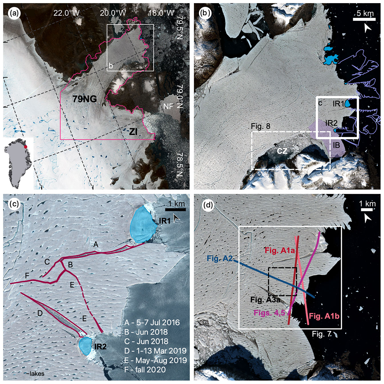
Figure 1 Overview of the eastern calving front of 79NG. Panel (a) displays 79NG and its location in Greenland. The pink line outlines the modelling domain. (b) The eastern calving front of 79NG with pinning points at the ice front shaded in blue. CZ indicates the southern chaos zone, and IB marks an ice bridge (see text for details). The boxes indicate subsets used in (c) and Fig. 8. The purple lines represent the calving front from 24 September 1980. (c) Red lines denote cracks as they were on 20 August 2022 with names A–F mentioned in the main text. The dashed line denotes that the crack does not intersect the ice in the vertical direction entirely. The legend gives the dates or time frame of crack formation. (d) Overview of the UWB profiles displayed in Figs. 5 and A1 (in reddish colour), the ALS profile from Fig. 4, the profile crossing Crack E from Fig. A2 (blue), and the area shown in Fig. 7 (white) and Fig. A3 (grey). The background images are from Sentinel-2: (a) 11 August 2021, (b, d) 2 September 2021 and (c) 20 August 2022.

Our aim is to investigate how and why calving at the eastern front of 79NG has changed. To this end, we detect calving front position, crack formation and propagation and compare this to principal stresses prior to the crack formation. Furthermore, we explore which role thinning of the floating tongue played in the retreat of the calving front. In a final step we assess which impact a further retreat of the calving front will have on 79NG's contribution to sea level change by means of numerical perturbation experiments.

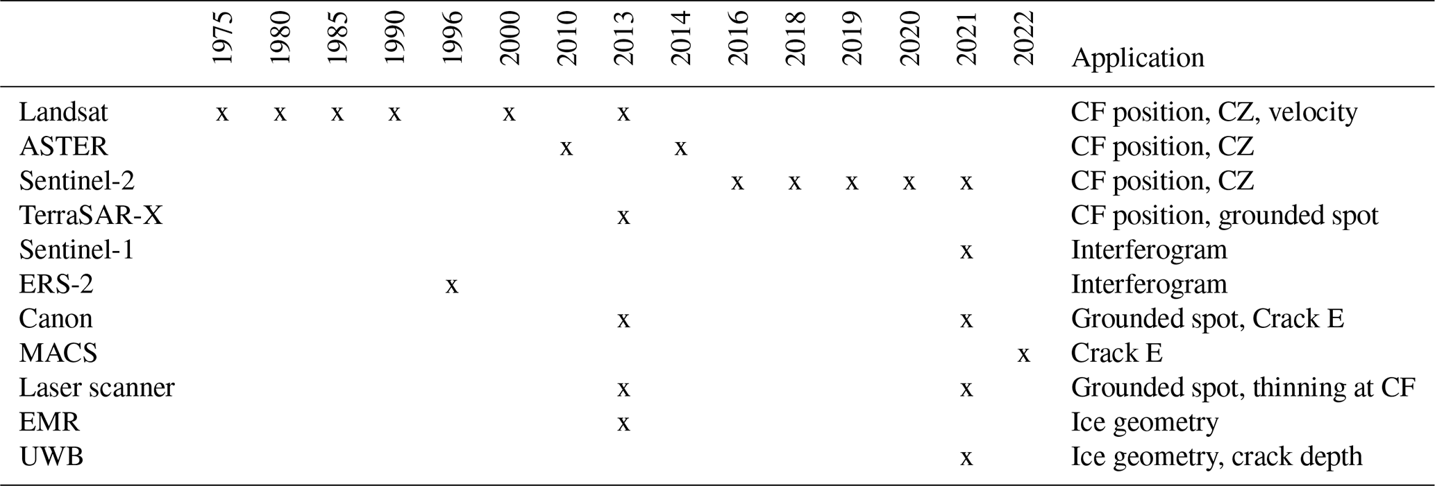
As our study relies on an extensive data basis, we provide an overview in Table 1. The last column of the table briefly summarizes what the data are used for. We mainly use optical, but also radar imagery, as well as synthetic aperture radar (SAR) interferometry and products such as velocity fields. Airborne data in this study comprise ice-penetrating radar (Electromagnetic Reflection System, EMR; ultra-wideband, UWB), airborne laser scanner (ALS) and optical imagery. For increasing the readability of the text, we present the details of the data processing only in Appendix A.

Table 1 Overview of the data used in this study in respective years. (CF: calving front position; CZ: chaos zone)

The observational datasets are complemented by numerical modelling simulations which aim to assess the instantaneous velocity response to a retreating floating tongue (Sect. 3 and Appendix B). Based on this variety of datasets we aim to investigate whether recent changes in 79NG indicate a regime change, what exactly the cause of the changes is and how this will impact the stability of 79NG.

The text is organized as follows: we first demonstrate that the calving style has changed, present a fracture-mechanical assessment of the floating tongue at the calving front and discuss the evolution of a weak zone that potentially influences the floating tongue stability. We continue with estimating the impact of future (large) calving events on 79NG's sea level contribution by means of ice flow modelling (details are presented in Appendix B). Finally, we compare our findings with disintegration or catastrophic calving/disintegration events at other floating tongues and ice shelves.

2 Transition in calving regime

Comparing the calving front locations in satellite imagery allows us to investigate whether the type of calving has changed. Figure 2 displays the calving front in 2000, 2010 and 2020. While in 2000 (Fig. 2a) a tongue exists between the two ice rises, and calving is initiated by the lateral rifts downstream of the ice rises IR1 and IR2, the calving front in 2020 (Fig. 2c) is characterized by rifts forming in the upstream direction (A and D in Fig. 2c).

Satellite imagery going back until 1975 shows that the tongue-type calving style has been present at least for 28 years until summer 2003. This is in line with the findings of Khan et al. (2014). After 2003, the calving front retreated to a nearly straight line between the two ice rises (similar to Fig. 2b) and remained in this shape until 2011.

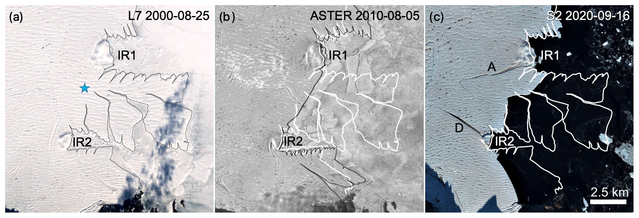
Figure 2 Evolution of the calving front and crack areas over 2 decades based on optical satellite imagery of (a) Landsat 7, (b) ASTER and (c) Sentinel-2 missions, respectively. The blue star denotes an area that has been partially grounded (see main text). In panels (a) and (b) the calving front is highlighted with a thin black line, and in (b) and (c) the calving front of panel (a) is superimposed in white colour.

Figure 2a indicates that the lateral rifts first grow towards the centre of the tongue (in across-flow direction) between the ice rises before changing orientation towards the spot marked with a blue star. This rift geometry, leading to tongue-type calving, is also found back to 1975, and until 2003 icebergs had been detached by these rifts, breaking L-shaped/wedge-shaped icebergs off.

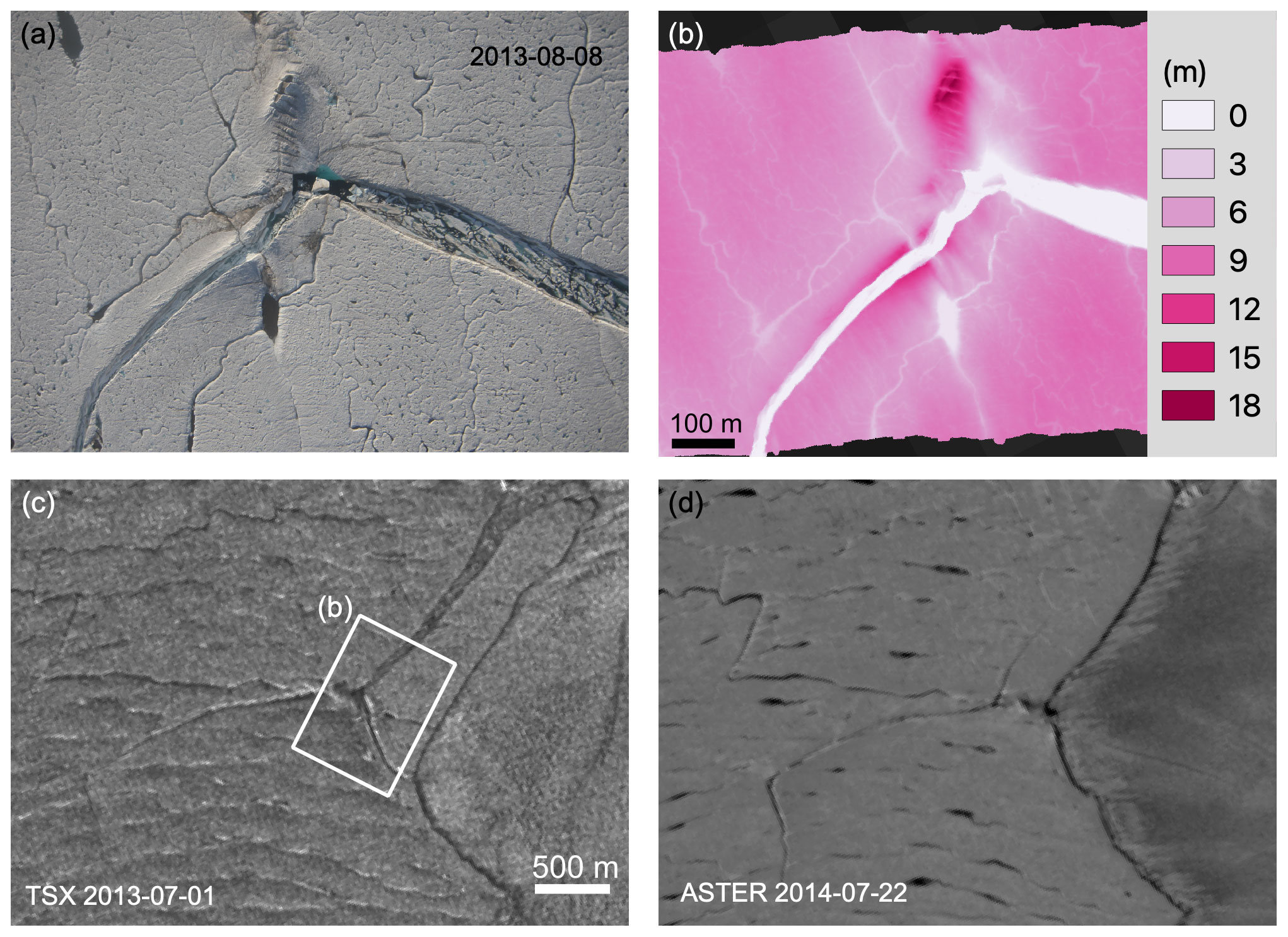
Figure 3 Former grounded spot. (a) Photo from the Canon camera on board Polar 5 crossing the grounded spot. (b) ALS surface elevation over at the same area as panel (a). The location of the profile is presented in Fig. 1d. Satellite imagery during grounding (c) and after ungrounding (d). Panels (c) and (d) show the area of panel (b) as an inset.

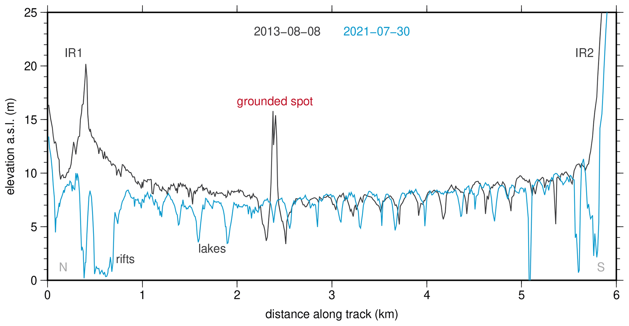
Figure 4 Thinning along a profile in the vicinity of the calving front between 2013 (grey line) and 2021 (blue line) based on ALS data. The location denoted by “grounded spot” corresponds to the same feature in Fig. 3, and the profile location is shown in Fig. 1d. Elevations below 3 m belong to rifts in the vicinity of ice rise margins.

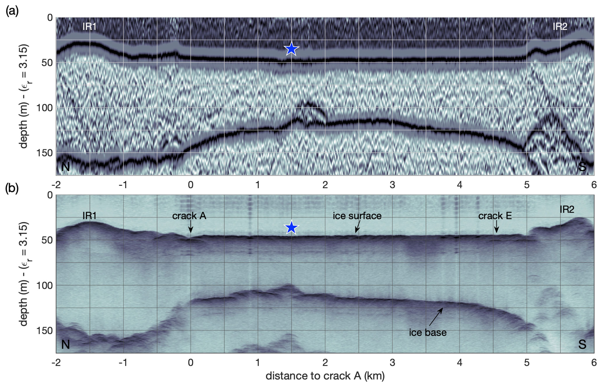
Based on the data analysed here, we suggest that between the two ice rises a small grounded spot at the location of the blue star (Fig. 2a) existed until 2013. That spot became ungrounded early in 2014. Our inference is based on the following observations: the surface structure as seen from the airborne optical camera on 8 August 2013 (Fig. 3a) is consistent with this spot being grounded as the surface elevation is 12 m higher than the surrounding floating tongue (ALS in Fig. 3b), and the flow velocity is low (Fig. 6d). Evidence for ungrounding of this location comes from different data sources: a comparison of satellite imagery from 2013 (Fig. 3c) and 2014 (Fig. 3d) shows that this surface buckle is moving downstream. Furthermore, ALS elevation data lack the dome-like structure at the same location in 2021 (Fig. 4). In 2013 the radargram clearly indicates reflection from a grounded spot, as presented in Fig. 5a. Interestingly enough, in 2021 ice-penetrating radar shows even thinner ice at the location that was formerly grounded (see Fig. 5; location of profiles shown in Fig. 1d). This further supports the argumentation that this area was ungrounding. Since 2013 such a dome-like structure was not newly formed, underlining this spot being in a transition to a new state. An episodic change between grounding and ungrounding seems to be rather unlikely based on our data. To conclude, we infer that a grounded spot existed at least for 4 decades and became afloat in early 2014.

Ungrounding can be a result of two processes: (i) thinner ice approaching the shallow bathymetry or (ii) thinning of the ice locally. Repeat ALS elevation data from 2013 and 2021 reveal a difference in the ice surface of about 1.5 m north and almost no change south of that grounded spot (Fig. 4). We are aware that the surface elevation difference is only slightly above the tidal range, expected to be in the range of 1 m based on measurements of Reeh et al. (2000), Christmann et al. (2021) and the FES2014b ocean tide model (Lyard et al., 2006); however, the thinning of the ice rises alone (left and right in Fig. 4) exemplifies that surface melting was taking place in these 8 years.

Figure 5 Airborne radar echograms recorded with (a) EMR radar from 2013 and (b) UWB radar from 2021 showing Cracks A and E. The location of the radargrams is shown in Fig. 1d. The blue star marks the location of the grounded spot found in ALS surface elevation from 2013 (Fig. 4).

In addition to the ungrounding, we observe severe changes in the crack evolution at the calving front over the last years/decades. For the sake of clarity, we have denoted each crack with a label from A to F (Fig. 1c). Between 5–7 July 2016 Crack A formed over a length of about 3 km and has widened since. The shorter Cracks B and C were formed 2 years later, in June 2018. Crack D formed at the southern ice rise between 1–13 March 2019 (3.5 km length). Both Cracks A and D are actually rifts that propagate through the full ice depth. The widening of both cracks over the course of 3 years is substantial: Crack A from 20 to 180 m between 9 September 2016 and 7 September 2019 and Crack D from 65 to 284 m between 2 September 2019 and 20 August 2022. The evolution of Crack E is more difficult to obtain from satellite imagery: between May and August 2019 it was formed in several episodes from two sides, starting from Crack B and IR2. Although Canon optical data show in 2021 that the northern and southern branches are close to joining (shown in high resolution in Fig. A3a, marked by a red arrow), there is no indication that they are rifts that propagate through the full ice depth, which we discuss below in more detail. The situation is similar in summer 2022, which is revealed by high-resolution imagery of the airborne Modular Aerial Camera System (MACS) presented in Fig. A3b. Crack F evolved in autumn 2020 and also propagated slightly in winter 2021/22. Crack C extended in early July 2022, while the crack at IR1 just north of Crack A propagated at the end of July 2022 towards the junction of Crack A (visible in Fig. 1c). Most importantly, the crack evolution reaches far upstream of the ice rises, marking the first event of this kind since the observational era at 79NG. Currently, the crack tip locations of the Cracks D and F are located about 5–7 km further upstream than the calving front in 2010. Despite not yet being calved off, the rifts are already now intersecting the ice, and as a consequence, the stresses in the floating tongue are changing, which is discussed below.

The crack and rift evolution presented above is a complex process for which we next develop a fracture-mechanical interpretation. We investigate the crack evolution and unveil the modes under which the cracks are formed and discuss how that changed in the recent past.

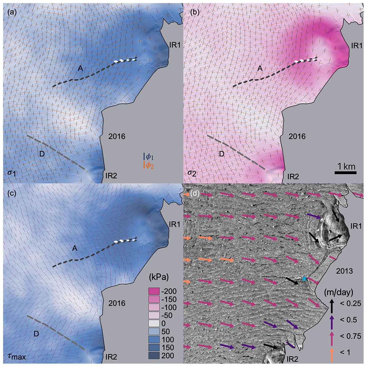
Figure 6 Principal stresses in 2016 and velocity field in 2013: (a) first principal normal stress, (b) second principal normal stress; crosses indicate principal stress directions (ϕ₁, ϕ₂). (c) Maximum shear stress; lines indicate the direction. (d) Velocity field in 2013 superimposed on a TerraSAR-X radar image. The blue star denotes the grounded spot. The dashed white line shows the initial Crack A and the black one its length after the propagation in 2016. The dashed grey line represents Crack D right after formation in 2019. The scale bar in panel (c) is valid for panels (a)–(c).

Figure 6 shows the first and second principal stresses between the ice rises with their corresponding directions calculated from a velocity field of 2014–2016 by means of inverse modelling. Furthermore, the figure displays the maximum shear stress and its direction. As pinning points act as barriers for the ice flow, their upstream side is characterized by compressive stresses. Consequently, shear zones exist between the compressive stress zone of each ice rise and the main flow between the two ice rises. The maximum shear stress descends towards zero in the main flow area. This setting enabled the formation of Mode II cracks, as Crack A is one. Crack A runs into an area with low stresses (principal as well as shear stresses), which is likely the reason for why the crack stops propagating (see Fig. 6).

To identify the mode of Crack D we cannot use any principal stress field, as due to a lack of data coverage, we only have a stress field prior to the formation of Crack A, and the initiation of Crack A very likely had a large influence on the stress field. We do however observe that the crack faces move apart, which is typical for Mode I cracks, as can be seen in Fig. 1c.

Interestingly enough, the direction of crack propagation is neither along surface rivers or lakes nor along remnants of historic crevasses. We only find one instance in the propagation of Crack A where the running crack joins a river shore for ∼200 m and deviates from it thereafter again. Crack arrest does not coincide with rivers or lakes, as we find evidence of cracks propagating across meandering rivers and lakes and propagating further. One may wonder why rivers and lakes do not disturb crack propagation. In comparison with the ice thickness of about 80 m a 1–2 m deep river or 3–4 m (based on ALS data) deep lake is still a minor change in thickness. From our perspective, this surface topography can be seen as a surface roughness, but without an additional stress concentration, a surface roughness alone does not control the propagation of a crack.

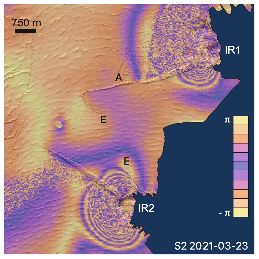
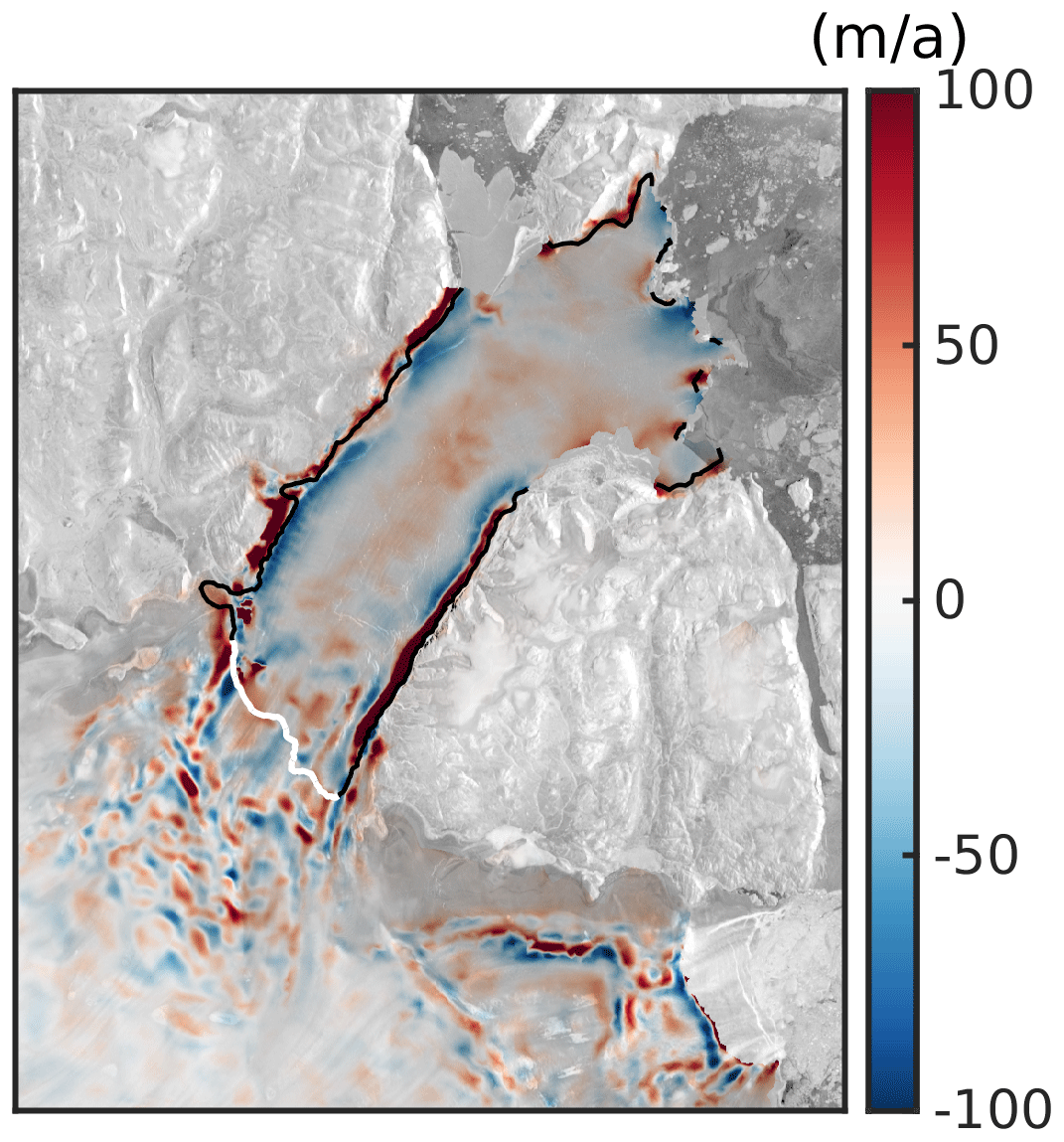
Figure 7 Double differential interferogram (14, 20 and 26 March 2021) based on Sentinel-1 and superimposed on a Sentinel-2 image of 23 March 2020. The colour denotes the phase difference.

The ice-penetrating radar data from 2021 (overview of flight lines is presented in Fig. 1d) across Crack E revealed that the crack does not intersect the ice entirely in the vertical direction at the end of July 2021 (Figs. 5, A1 and A2). However, surface imagery (Fig. A3) from the onboard camera in 2021, as well as optical satellite imagery (see Appendix A), shows a thin surface crack at the same time (dashed line in Fig. 1c). In summer 2022, we find lakes ponding over this thin line, and the surface ponds are not drained by Crack E. Forming a vertically non-intersecting crack is characteristic for a fatigue fracture. Fatigue fractures are initiated from cyclic-loading situations on short timescales. The principal normal stresses between the ice rises are sufficiently low (Fig. 6a, b) to allow the existence and propagation of fatigue cracks. Here, tides are suggested to be the reason for the cyclic-loading situation. To support this, we explore fringe patterns of interferograms from March 2021 (Fig. 7). Remarkably, there are clear hinge zones around IR1 and IR2, despite the fractures intersecting the ice vertically. We suggest that at IR2, the floating ice tongue is pushed intensively against the ice rise, building a solid contact between the floating and grounded ice. At IR1, we suggest that there are still some intact connections between the floating part and the grounded ice of IR1. As a result, the deflection of the ice plate is a relative motion in the vertical direction, which leads to cyclic loading at Crack E. This deflection is presumably small enough so that the crack is not yet critical, otherwise the crack would have propagated through the entire ice thickness already.

None of the cracks are a hydrofracture. Hydrofractures are basically crevasses (pre-existing fractures) filled with water, either from surface melt draining into them, as on Antarctic ice shelves (e.g. Scambos et al., 2000), or facilitating supraglacial lake drainage (e.g. Das et al., 2008; Chudley et al., 2019). Cracks A–D and F are newly formed cracks that grow vertically and horizontally at once; they are rifts. As an example, Crack D was initiated in March, when no meltwater was available at all. Also, the newly formed cracks do not follow the remnants of old crevasses, which hydrofractures would have done. Crack E is the only crack that has the potential to become a hydrofracture. Formed in 2019, it has so far survived 3 years without propagating vertically through. Although the floating tongue at the calving front is densely covered with melt ponds in summer, the lakes are small and shallow, so the stress due to the water filling the crack has not yet been large enough to initiate hydrofracture. Hence, we conclude that the rifts are not hydrofractures but are initiated by stresses (not due to water pressure) exceeding the material strength.

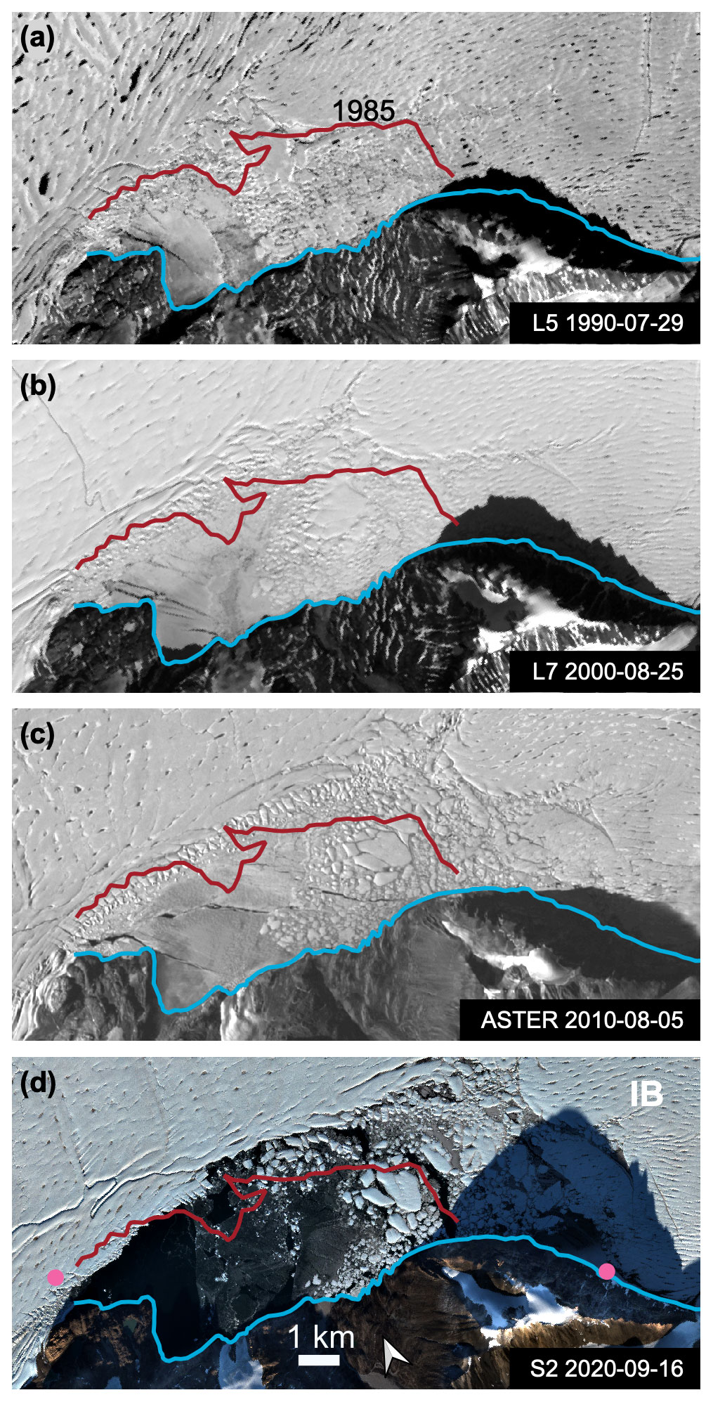
Figure 8 Evolution of the chaotic zone since 1990 in optical imagery (Landsat 5 and 7, ASTER, and Sentinel-2). The blue line marks the shore line, and the red line denotes the calving front from 1985. In panel (d), the pink dots mark an area without a hinge zone in interferograms.

We further consider the potential future evolution of the calving front. We anticipate that calving along the Cracks D, F, C and A will detach about 20 km² of ice but leave the ice bridge (IB; light purple in Fig. 1b; area ∼55 km²) unaffected. The remaining ice bridge has a calving front on both sides, one facing towards the open ocean to the east and another one towards a bay in the west. The southern calving front produces icebergs of smaller size that are trapped in the bay, encapsulated in winter by a seasonal mélange, whereas in summer this mélange opens up. We denote this area the “chaos zone” (CZ in Fig. 1b) and next investigate the evolution of this zone, which we display in Fig. 8. In 1990 this zone consisted of 14 km² of open area and a further 17 km² of fractured ice. In 2000 the open area including icebergs was 21 km², about 19 km² of which was fractured. This increased to 38 km² and 16 km² of open and fractured area, respectively, by August 2010. In September 2020, the open area was 50 km², 15 km² of which was fractured. The total area increased by 34 km², or 52 %, within 30 years, with 18 km² in the time when tongue-type calving was last observed, which was in 2004. Furthermore, the area of the calving front of this CZ has almost doubled, from 15 to 28 km². The extent of the ice bridge in the flow direction developed from 7.5 km² in 1996 to 5 km² in 2013 and 2016 to 3.8 km² in 2021, which is half the width in 25 years, with 35 % of loss in the past 5 years.

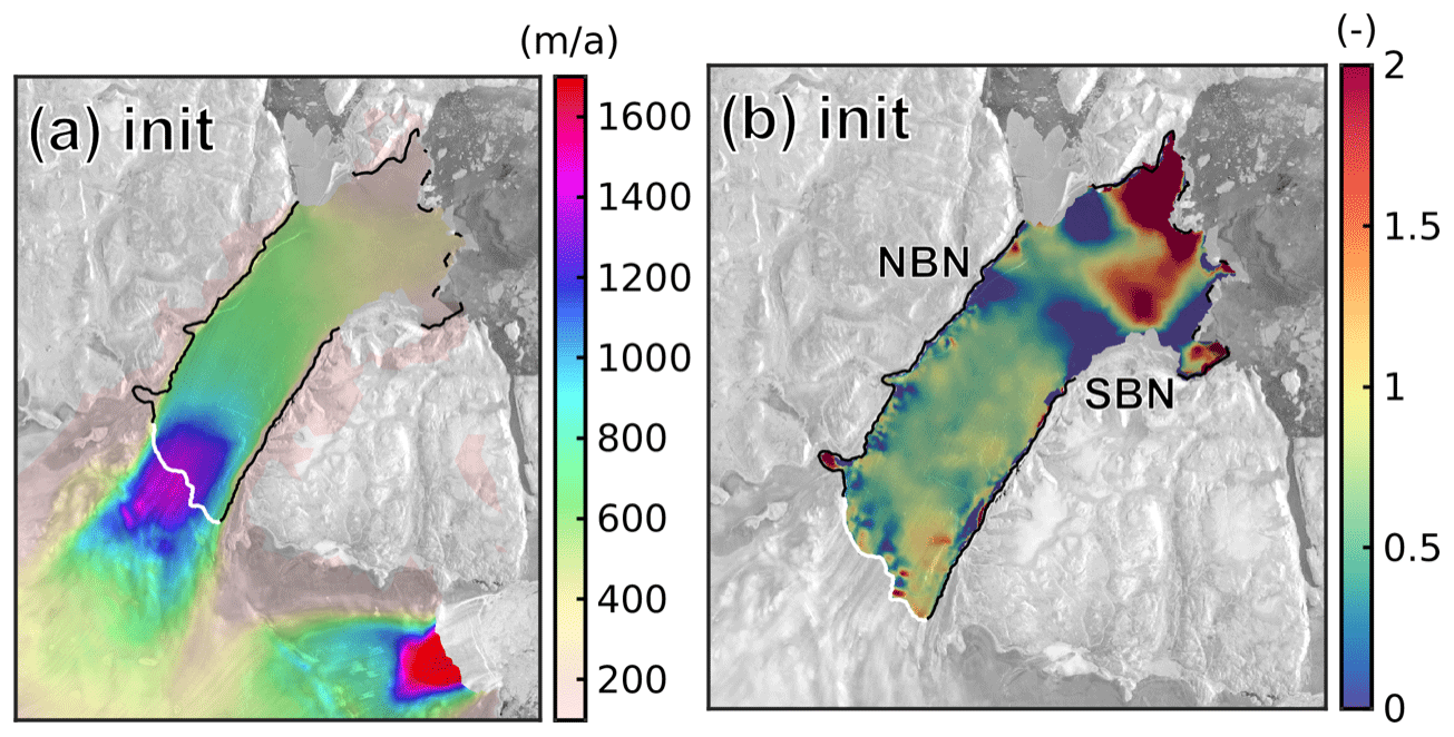
Figure 9 Simulation results of the ice flow model for init experiments Panel (a) shows simulated surface velocities. Panel (b) shows the buttressing parameter according to Borstad et al. (2013). A value of 0 represents an unbuttressed floating tongue, a value of 1 represents a fully buttressed floating tongue, and a value of >1 represents an overbuttressed ice shelf (i.e. longitudinal stresses are negative, i.e. compressive). The black line indicates the grounding line from the init state and the white line the main grounding line at which we compute grounding line flux.

The situation of the ice bridge at 79NG is comparable to the ice bridge at Wilkins Ice Shelf (WIS) in Antarctica, where a similar bridge was formed between stabilizing islands (Braun et al., 2009). The WIS ice bridge also had two calving fronts; one was supported by a thick ice mélange, while the other only had open ocean or winter sea ice and thus no support. The ice bridge had a width of 6 km² prior to its rupture and collapsed in 2008. The ice bridge at 79NG is narrower than the one at WIS but has the “advantage” that two smaller glaciers from the south drain into the ice bridge (see Fig. 1b, d). This leads to compression, which is visible in optical imagery and ALS elevation as a bulging zone (Fig. 1d).

3 Impact – response of 79NG instability of the calving front

As NEGIS is a fast-flowing ice stream and drains a large area of the GrIS (17.23 %; Krieger et al., 2020) it has the potential to contribute to sea level rise by an increased ice discharge once the boundary conditions, such as its calving front, change. We address the question of how future large calving events or even a large disintegration event will modify the ice discharge by using the Ice-sheet and Sea-level System Model (ISSM; Larour et al., 2012). According to Rückamp et al. (2022), we employ the full-Stokes (FS) model with a resolution of up to 200 m at the grounding line. We initialize the model using observational data of surface and basal topography as a target to determine the initial conditions by running a joint inversion for the basal friction coefficient and bulk ice rigidity of the ice (see Appendix B). The modelling domain is outlined in Fig. 1a. The initialization experiment is denoted init and reveals a root mean square error (RMSE) of 21.7 m a⁻¹ in the grounded part and 48.9 m a⁻¹ in the floating part (a map view of velocity differences is shown in Fig. B3). The init experiment reveals a grounding line flux of 11.9 Gt a⁻¹ (Fig. 9a; note that grounding line fluxes are computed across the main grounding line (white line)).

In order to estimate the back stress exerted by the floating tongue, we calculate a normalized buttressing parameter, f, following the method presented by Borstad et al. (2013). Besides geometric and rheologic parameters the buttressing parameter is calculated from contributions of lateral and shear strain rates. In the end, a value of f=0 corresponds to an unbuttressed ice shelf, while a value of f=1 represents a fully buttressed ice shelf. Values above 1 represent an overbuttressed ice shelf (i.e longitudinal stresses are negative, i.e. compressive). Up to the bottleneck (northern bottleneck, NBN, to southern bottleneck, SBN, in Fig. 9b) the floating tongue is currently nearly fully buttressed. Downstream of the bottleneck a band of unbuttressed ice exists. The area around the eastern calving front is mainly overbuttressed as a result of the existence of the ice rises.

We do not intend here to simulate future calving events and their impact on the long-term behaviour. We are interested in assessing the instantaneous glacier acceleration and increase in grounding line flux to future calving events. Therefore, we perform three diagnostic perturbation experiments in which we remove sections of 79NG's ice tongue. These experiments must not be treated as a snapshot in time of the future evolution, as they do not include any response to changes in oceanic or atmospheric forcing.

The first experiment calv-iceberg retreats the calving front position in order to replicate a potential calving event following Crack A towards the front of the chaos zone. The second experiment calv2fjord investigates a larger change in the floating tongue, whereby we assume that the calving front retreats up to a point where the fjord geometry narrows (denoted SBN and NBN, respectively, in Fig. 9b). This scenario mimics a sudden collapse of the frontal part, i.e. 46 % of the floating tongue area. A full collapse of 79NG's floating tongue is assumed in a third scenario, collapse. Next to the simulation results the detached parts are shown in Fig. 10 as purple shading.

With loss of the connection to the two southern ice rises the experiment calv-iceberg leads predominantly to ice flow increase (Fig. 10a). In the vicinity of the newly developed ice front a speed-up of 118 m a⁻¹ is simulated. Compared to the init experiment only the northern tip of the calving front remains overbuttressed, while the central part of the floating tongue remains in a similar state (Fig. 10d). This scenario shows a grounding line flux of 12.0 Gt a⁻¹, which is an increase of 0.2 %. With a further retreat (calv2fjord) the situation changes dramatically into an almost entirely underbuttressed floating tongue (Fig. 10e). This comes along with a speed-up of the floating tongue of up to 446 m a⁻¹ (Fig. 10b) and an increase in ice discharge of 5.1 % (12.5 Gt a⁻¹) compared to the init experiment. Eventually, the full collapse experiment further enhances the speed-up upstream of the grounding line up to 2448 m a⁻¹ (Fig. 10c). This leads to a 166 % (31.6 Gt a⁻¹) increase in the grounding line flux. Comparing the experiments with each other, it becomes evident that there is a substantial difference between calv-iceberg and calv2fjord. In calv-iceberg the floating tongue still has a pinned front; thus the ice is still slower at the calving front than at the grounding line. In the experiment calv2fjord the velocity at the new calving front is much higher, which leads to the highly underbuttressed area near the front.

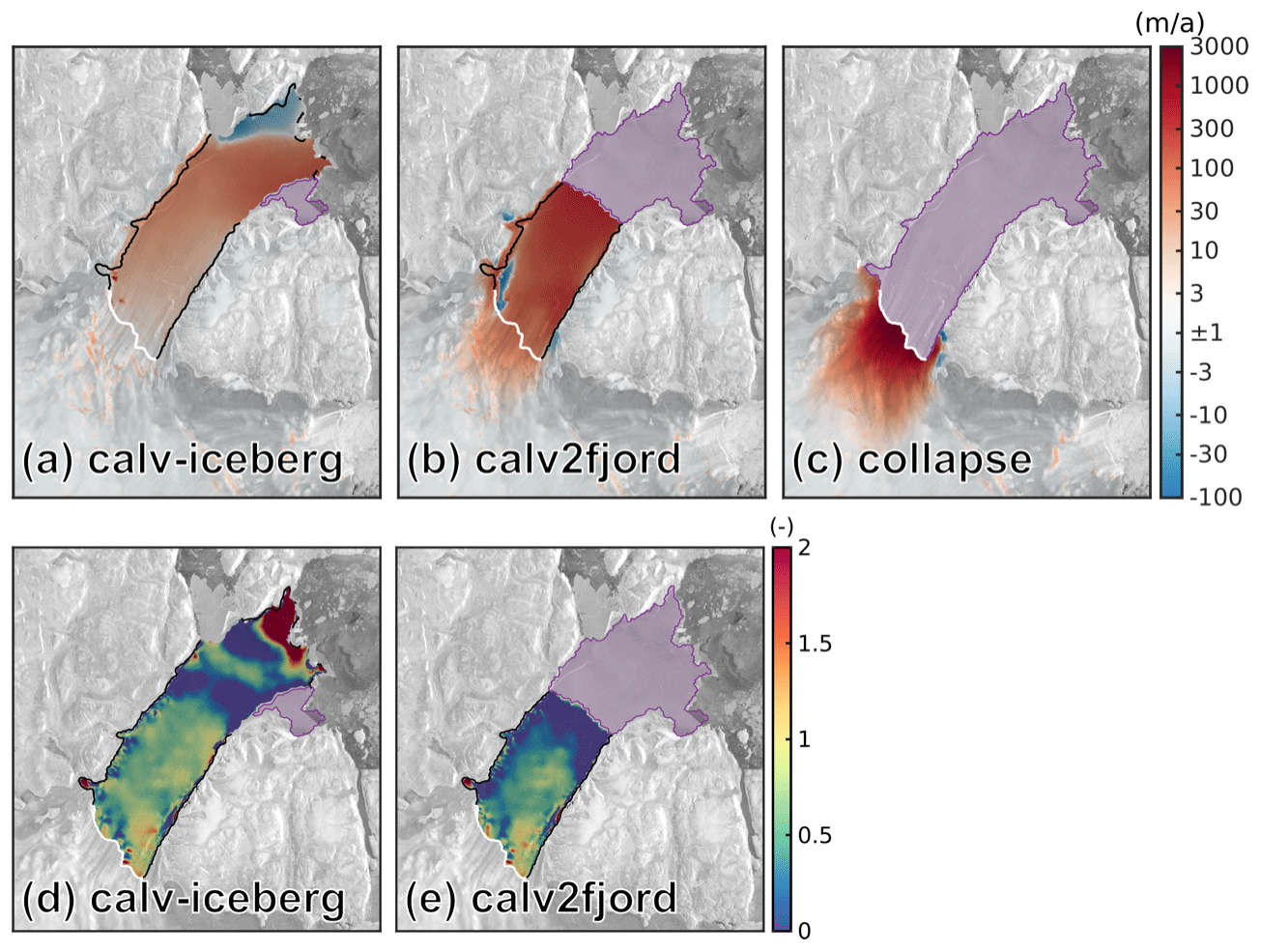
Figure 10 Simulation results of the ice flow model for the three perturbation experiments. Panels (a), (b) and (c) show velocity differences in the calv-iceberg, calv2fjord and collapse experiments to simulated velocities from the init experiment, respectively. Panels (d) and (e) show the buttressing parameter according to Borstad et al. (2013). A value of 0 represents an unbuttressed floating tongue, a value of 1 represents a fully buttressed floating tongue, and a value of >1 represents an overbuttressed ice shelf (i.e. longitudinal stresses are negative, i.e. compressive). The black line indicates the grounding line from the init state and the white line the main grounding line across which we compute grounding line flux. The detached parts for each experiment are highlighted with purple shading.

4 Discussion

We start by comparing the situation at 79NG's eastern calving front with other ice shelves and floating tongues that have features similar to the ones at 79NG and have undergone considerable change in which these features played a role. First we discuss the WIS, which is mentioned above.

The ice bridge at WIS was much wider, and the confining islands also had a larger size, leading to a broader contact with the confining margins. That ice bridge remained intact in its narrowest form for about 12 months, after which shattering of the ice bridge (Humbert et al., 2010) triggered a sequence of fast crack evolution before today's calving front settled in 2009. This can inform us about the timescale at which we shall expect events at 79NG's calving front to happen. Although 15 % of the ice shelf area was lost in only 14 months, a new, potentially intermediate state has been reached that has remained now for more than a decade.

Jakobshavn Isbræ (JI) has retreated past a lateral embayment of the fjord, and we intend here to investigate if that situation is comparable to 79NG's chaos zone shown in Fig. 8. At JI the embayment had a length of about 12 km, with an ice rise located at ∼5 km, forming a shear margin between the fast glacier flow and the embayment with almost stagnant ice (Joughin et al., 2004). The retreat across this embayment from the ice rise upstream took place in less than 10 months. It is important to note that the embayment was entirely filled with glacier ice (Csatho et al., 2008), even with buckling along its margin, whereas at 79NG, the zone is only filled with icebergs and seasonal sea ice, making it much easier to retreat past this area. Comparing the retreat of the calving front of ZI with 79NG, it becomes evident that most of the retreat of ZI appeared in a zone that was already highly heterogeneous in the 1980s (Thomas et al., 2009; Khan et al., 2014). The northern part of 79NG's eastern calving front is somewhat similar to ZI's north-eastern part (see Fig. 1a, marked with NF), as both are stagnant and show similar surface buckling. In our simulations, this area is overbuttressed at 79NG (see Fig. 10), which one could argue too for ZI's north-eastern part, which still exists after the massive retreat of ZI's calving front.

In all three cases, WIS, JI and ZI, the events took place on short timescales, so only days to months after the disintegration has been triggered. This may partly have been due to the fact that ice is a brittle material, and fractures propagate very fast (about a third of the speed of sound), but more prominently that ice responds to change in stress state on short timescales elastically (e.g. Christmann et al., 2021). Once a change in the calving front situation occurs the elastic stress is redistributed instantaneously and can trigger further follow-up events as well as lead to a modified viscous response over months to years; see Rankl et al. (2017) for WIS.

However, similar to the fact that WIS has not retreated further to date despite a high number of annual melt days (Johnson et al., 2022), and JI's calving front retreat and acceleration have slowed down (Joughin et al., 2020), 79NG may retreat in episodes.

Other glaciers in the north and north-east, for example Ryder Glacier, Brikkerne, Hagen Bræ and Kofoed-Hansen Bræ, show an even more complex behaviour than we discuss here for 79NG, as they are potentially of the surge type (Hill et al., 2017), while no evidence for surges is found for 79NG and ZI.

Next, we consider different external drivers that might have contributed to the changes observed at the calving front, such as air and ocean temperatures. The changes in air temperature across Greenland have recently been analysed by Zhang et al. (2022). They present data from the weather station in Danmarkshavn, some 300 km south of our study area, from 1958–2020, which show a step in 2 m temperatures of more than 1 ^∘C in the mid-1990s. This makes thinning of the floating tongue at the calving front more likely to arise from increased surface melting than due to oceanic forcing. Schaffer et al. (2020) found warm water inflow into the cavity of 79NG at 400 m depth, which would thus not come into contact with the ice base at the calving front, consequently also leading to low basal melt rates, as shown by Wilson et al. (2017).

5 Conclusions

By means of remote sensing data, we detect changes in 79NG's eastern calving front that suggest the onset of destabilization. Crack evolution is initiated at prominent ice rises and progresses far upstream. We identified crack initiation by shear mode, while crack propagation is in Mode I and Mode II for Cracks D and A, respectively. Interestingly, Crack E is none of these but could be a fatigue crack due to tidal forcing. As these crack patterns are very distinct from normal tongue-type calving we speculate that the new crack formations are a precursor to disintegration. Moreover, we present evidence for ungrounding of a small pinning point due to thinning of the ice thickness after 2013. Basal melt rates are presumably small along the calving front, making thinning by surface melting a likely driver for this change. Changes are ongoing not only at the eastern calving front, but also at the southern margin of the floating tongue: in 2022 this margin had a calving front almost twice as long as in 1985. The frontal part of 79NG is thus weakened from both sides. An area of ∼5 % of the floating tongue is likely to be lost in the near future. Numerical ice flow simulations show that the loss of such a relatively small area leads to an increase in the grounding line discharge of about 0.2 % due to the reduction in the exerted buttressing. A sudden collapse of about 46 % of the floating tongue further destabilizes the glacier and will increase the ice discharge of 79NG by 5.1 %. Eventually, a full collapse of the floating tongue increases the grounding line flux by 166 %. Our findings indicate that 79NG is potentially at the onset of a major retreat phase.

Appendix A: Data

A1 Satellite data

For the analyses in this paper, we explore a range of different satellite sensors. Optical Landsat 5, 7 and 8 as well as ASTER and Sentinel-2 imagery is used to derive time series of calving front evolution. For this purpose, we use the radiometrically calibrated and orthorectified Landsat Level-1 products provided by the United States Geological Survey and the Sentinel-2 Level-2A products provided by Copernicus, respectively.

Furthermore, we use Landsat 8 imagery to determine ice flow velocity. This is realized through a combined feature tracking approach. We utilize the fast normalized cross-correlation as well as a subsequent least-squares matching in order to estimate displacement vectors with subpixel accuracy. A detailed description of the processing system is given by Rosenau et al. (2015).

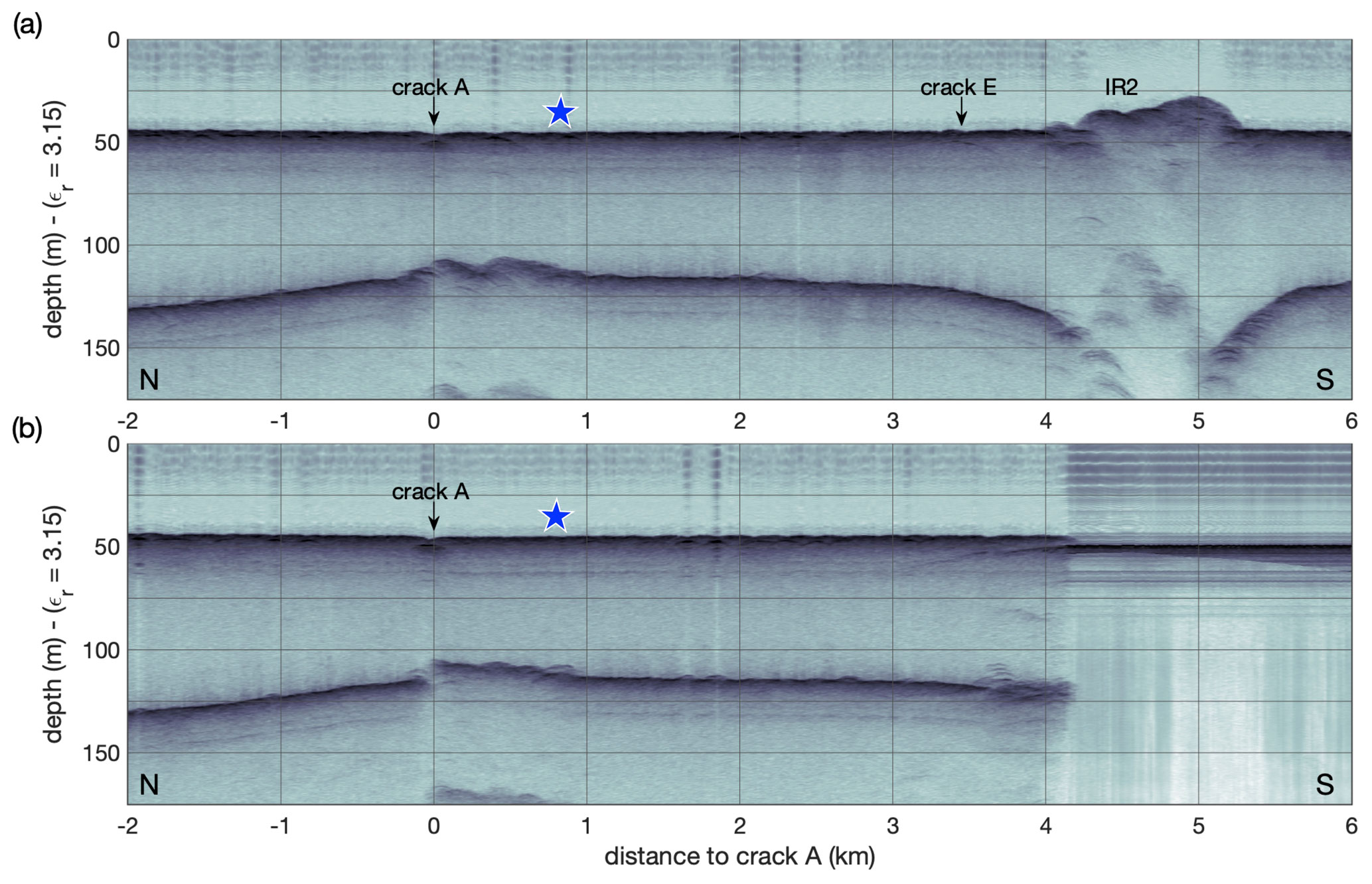
Figure A1 Airborne UWB radar echograms from 2021 recorded in the study area and crossing today's Crack A. The location of both profiles is shown in Fig. 1. The first strong reflection represents the ice surface and the second one the ice base. The blue stars mark the location of the grounded spot found in Fig. 5a and in ALS elevation data from 2013 (Fig. 4).

Sentinel-1 synthetic aperture radar (SAR) imagery is used for detecting calving front and crack positions. For this purpose, the data were first radiometrically calibrated, and subsequently a range-Doppler terrain correction was applied using the GIMP terrain model (Howat et al., 2014). We intentionally do not apply speckle filtering in order to avoid smoothing of cracks. Mostly we use descending tracks with the relative orbit 170, which we found most useful for detecting crack evolution due to its orientation relative to the cracks. We use one TerraSAR-X scene in stripmap mode as an enhanced ellipsoid-corrected (EEC) product that has been reprocessed to 12.5 m resolution with a bicubic spline interpolation.

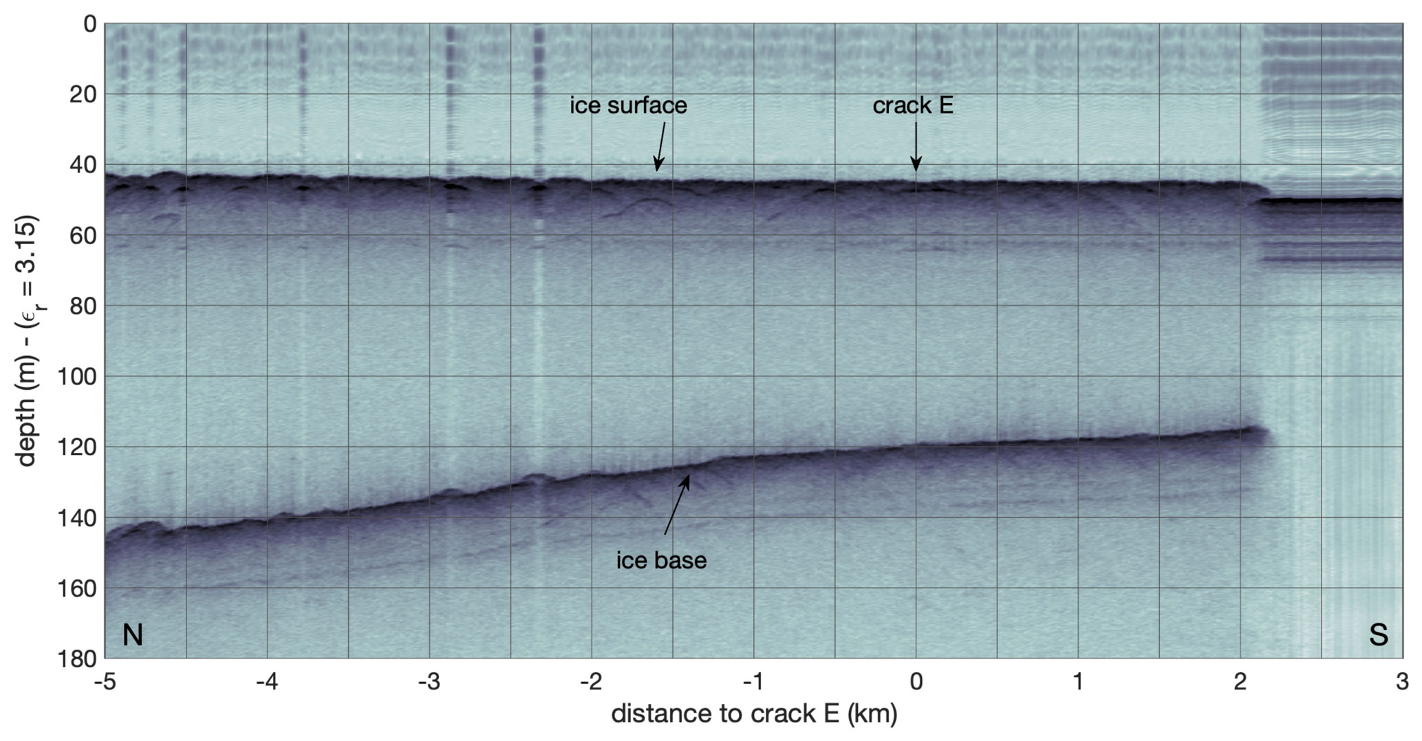
Figure A2 UWB echogram from 2021 crossing Crack E. For orientation: flight direction is towards the calving front, which is located 2 km from Crack E. The first strong reflection represents the ice surface and the second one the ice base. The location of the profile is shown in Fig. 1d.

With the availability of high-resolution SAR data with frequent revisiting times, SAR interferometry (InSAR) became an important tool for monitoring the evolution of cracks on floating ice shelves (e.g. Rückamp et al., 2019; Libert et al., 2022). Here, we applied SAR interferometry to Sentinel-1 interferometric wide (IW) data following Neckel et al. (2021). In a first step, continuous single-look complex (SLC) images were generated from each set of bursts and swaths. SLC images of orbit 170, slice 2 were co-registered with the help of precise orbit information and the global TanDEM-X DEM gridded to 30 m spatial resolution (Wessel et al., 2016). The accuracy of the co-registration was further refined by employing an iterative offset tracking approach between both SLCs. This is essential in fast-flowing regions where phase jumps in burst overlap areas are most common. Two repeat-pass interferograms were generated with data acquired on 14, 20 and 26 March 2021. Topography-induced phase information was removed from both interferograms employing the global TanDEM-X DEM. To minimize the effect of static horizontal ice flow a double differential interferogram was created, which is shown in Fig. 7.

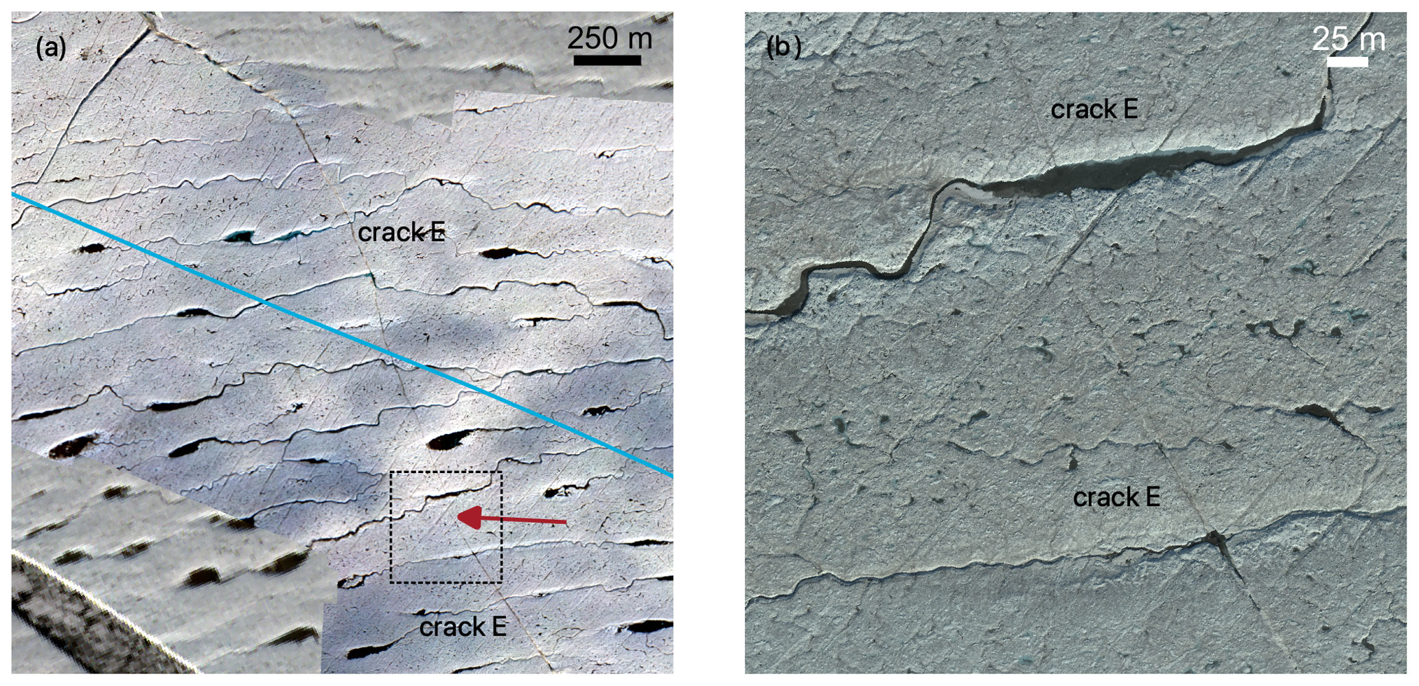
Figure A3 (a) Mosaic of the onboard optical Canon camera from a flight on 30 July 2021 superimposed on a Sentinel-2 image of the same date. The red arrow points to the location of the crack tips at the surface. The flight track from Fig. A2 is shown as a blue line. Note that the rivers and lakes through which the narrow Crack E has propagated are not drained, pointing out that the crack is not extending through the entire ice thickness. (b) Mosaic of the MACS-Polar camera from a flight on 20 August 2022. The area of panel (b) is shown in panel (a) as a dashed box.

A2 Ice-penetrating radar

We used the ultra-wideband (UWB) Multichannel Coherent Radar Depth Sounder (MCoRDS, version 5) on board the polar aircraft Polar 5 of the Alfred Wegener Institute Helmholtz Centre for Polar and Marine Research (AWI). The UWB has an array of eight antennas with a total transmit power of 6 kW and can be operated in the frequency band of 150–600 MHz (Hale et al., 2016). The radar was operated with a pulse repetition frequency of 10 kHz and a sampling frequency of 1.6 GHz. We used alternating sequences of different transmission/recording settings (waveforms) to increase the dynamic range: short pulses (1 µs) and low receiver gain (11–13 dB) to image the glacier surface and longer pulses (3 and 10 µs) with higher receiver gain (48 dB) to image internal features and the ice base. The waveforms were defined with regard to the thickness of the floating tongue. In our survey we used a bandwidth of 370 MHz within the frequency band of 150–520 MHz. Post-flight processing included pulse compression in range direction and synthetic aperture radar focusing on the along-track direction. The final along-track resolution was set to 10 m. We assumed a relative permittivity of ε_r=3.15 in ice for the time-to-depth conversion. The theoretical range resolution in ice after pulse compression for the chosen bandwidth is about 0.23 m. As there is no thick firn layer, we did not apply any firn correction. We concatenated the echograms of the alternating waveforms to obtain the final echograms covering the ice from the surface to the base with high dynamic range. Figure 1d gives an overview of the ice-penetrating data used in this study.

In addition and to compare to the more recent UWB system (Fig. A1) we used data from the Electromagnetic Reflection System (EMR). The EMR is an airborne radio-echo sounding system used to map ice thicknesses and internal layering of glaciers, ice sheets and ice shelves. The system is capable of penetrating 4000 m thick ice. It was designed and built by AWI in cooperation with Aerodata Flugmeßtechnik GmbH, Hamburg University of Technology and the Deutsches Zentrum für Luft- und Raumfahrt e.V. (DLR). The radar signal is a 150 MHz burst with a signal length of 60 or 600 ns. The maximum performance is 1.6 kW, with a sensitivity of 190 dB (Nixdorf et al., 1999).

A3 Global navigation satellite system (GNSS)

The aircraft's position was measured using a dual-frequency NovAtel OEMV GNSS receiver at a sampling rate of 20 Hz. To determine the flight trajectory we use the precise point positioning (PPP) post-processing option including precise clocks and ephemerides of the commercial GNSS software package Waypoint 8.90. The accuracy of the post-processed trajectory is less than 0.1 m but varies along-track.

A4 Laser scanner

Airborne laser scanner (ALS) data were acquired in 2013 and 2021 with the laser scanner system (RIEGL LMS-VQ580) and a scan angle of 60^∘. The aircraft was flying roughly 300 m above ground, resulting in a scan width of about 300 m and a mean point-to-point distance of ∼0.5 m. To obtain the final calibrated geo-referenced point cloud (PC) data, the raw laser data were combined with the post-processed GNSS trajectory, corrected for altitude of the aircraft and calibration angles. Crossovers were used to calibrate the system and to derive the elevation accuracy of the final geo-referenced PC to be better than 0.1±0.1 m. The bias of <0.1 m varies along-track and is due to the vertical accuracy of the post-processed GNSS trajectory. The final digital elevation model (DEM) with 1 m horizontal resolution was derived from the PC by using an inverse distance weighting (IDW) algorithm and a 5 m search radius. Finally, the freeboard was obtained by reducing the ALS DEM, which has been referenced to WGS84, to the EGM2008 geoid (Pavlis et al., 2012).

Please note that no tidal correction has been applied to the 2013 and 2021 DEMs. The tidal elevation is expected to be in the range of 1 m based on the measurements of Reeh et al. (2000) and Christmann et al. (2021) and the FES2014b ocean tide model (Lyard et al., 2006).

A5 Red–green–blue (RGB) camera data

Next to the ALS data a nadir-looking CANON EOS-1D Mark III digital single-lens reflex (DSLR) camera in combination with a CANON 14 mm f/2.8L II USM lens is routinely employed on board AWI's research aircraft. RGB images are acquired at 6 s intervals and are stored together with a GNSS time tag in RAW data format. We selected all images acquired in the vicinity of the crack location and assigned the temporally closest dual-frequency GNSS and inertial navigation system (INS) measurement to each image. All images were then corrected for vignetting effects and converted into JPG format preserving the original high resolution. In the next step we employed the structure-from-motion pipeline of the commercial Agisoft Metashape software (Beyer et al., 2018) to obtain a high-resolution DEM and orthomosaic of the 2021 crack area. In order to match the orthomosaic with the temporally consistent ALS DEM we co-register both DEMs and employed the derived translation and rotation information to transform the final orthomosaic image. The resulting mosaic is displayed in Fig. A3a.

A6 MACS-Polar

The Modular Aerial Camera System (MACS) is a family of optical sensor instruments specifically developed for scientific application in unusual environments. Based on a modular software and hardware design, various project-related demands like geometric and radiometric configurations as well as assembly constraints can be realized. To be carried by AWI’s polar aircraft and to be operated in cold regions, a special version named MACS-Polar was established. The sensor head was separated from the control-and-logging unit. Thus, the sensor head consisting of cameras and an inertial measurement unit (IMU) was mounted underfloor in the fuselage, while the cabin-mounted data logging unit remained accessible during the campaign. For ice monitoring, a downward-oriented sensor configuration was chosen, acquiring images in various optical bands. The RGB spectrum is valuable for characterization of melt ponds and for the visual interpretation of the scene by humans. From an altitude of 1000 m above ground level the optical configuration yields a ground sampling distance (GSD) of 0.15 m in the RGB. In this case the swath width is 700 m. All three cameras take images at the same time and with a continuous rate of up to four frames per second. This enables sufficient along-track image overlap of more than 80 % even while flying at very low altitudes less than 300 m. The frame rate is required to achieve a ground pixel resolution better than GSD =0.05 m. As MACS is a photogrammetric aerial camera, sensors are geometrically and radiometrically calibrated. In conjunction with the inertially aided geo-referencing system, all necessary parameters like geographic position, orientation and absolute time of every image’s pixel are known. The derivation of a true orthophoto follows the common photogrammetric approach. First, the aerial triangulation is performed with the initially known approximations of exterior orientation parameters of each image and their a priori accuracies to get the precise and accurate relationships between the individual image coordinate systems and a defined datum and projection. The surface elevation of the glacier is required for the correct positioning of individual colour pixels. The resulting mosaic for the crack tip of Crack E is displayed in Fig. A3b.

Appendix B: ISSM set-up

The ice flow modelling of the NEGIS is conducted with the Ice-Sheet and Sea-level System Model (ISSM; Larour et al., 2012). We employ the full-Stokes (FS) model as it was shown to be the most accurate (Rückamp et al., 2022). Model calculations are performed on an unstructured finite-element grid with a varying horizontal resolution between 0.2 and 10 km (Fig. B1). The base mesh consists of 1000 m resolution refined to 200 m next to the main grounding line over fast-flowing ice at 79NG (i.e. >300 m a⁻¹) and at the frontal pinning points. The domain is vertically extruded, with 15 layers refined to the base.

Figure B1 Horizontal mesh resolution (km). Data are clipped at 0.4 and 2 km. The horizontal resolution of a triangle is defined by its minimum edge length. The black line delineates the grounding line.

We initialize the model using the present-day ice geometry from BedMachine Greenland version 4 (Morlighem et al., 2017). We reconstruct basal friction, k², and bulk ice rigidity, B, using data assimilation of satellite measurements of surface ice velocity (Fig. B2) (AWI-S1 velocities as in Krieger et al., 2020, but with Sentinel-1 winter (November–March) data from the years 2014 to 2016). Since the surface velocity field has a different coverage to the BedMachine mask, we clipped the calving front to the coverage of the surface velocity field. We use a friction power law (Budd-like) on grounded ice that relates the basal shear stress, τ_b, to the sliding velocity, v_b,

$$\begin{array}{}\text{(B1)}& {\mathit{\tau }}_{\mathrm{b}}=-N^{\mathrm{1}/m}{k}^{\mathrm{2}}{\left|{\mathit{v}}_{\mathrm{b}}\right|}^{\mathrm{1}/m-\mathrm{1}}{\mathit{v}}_{\mathrm{b}},\end{array}$$

with the stress exponent m=3. The effective pressure, N, is assumed to be the difference in ice overburden pressure, p_i, and the subglacial water pressure, p_w, i.e. $N=p_{\mathrm{i}}-p_{\mathrm{w}}$. The basal water pressure is computed in marine parts, i.e. where the ice base, z_b, is below the sea level (z_b<z_sl), that is $p_{\mathrm{w}}=-min({\mathit{\varrho }}_{\mathrm{w}}g{z}_{\mathrm{b}},\mathrm{0})$, where ${\mathit{\varrho }}_{\mathrm{w}}=\mathrm{1023}\mathrm{kg}{\mathrm{m}}^{-\mathrm{3}}$ is the density of the ocean water.

The viscosity is given by the Glen–Steinemann flow law (Glen, 1955; Steinemann, 1954):

$$\begin{array}{}\text{(B2)}& \mathit{\eta }={\displaystyle \frac{\mathrm{1}}{\mathrm{2}}}B{\dot{\mathit{\epsilon }}}_{\mathrm{e}}^{(\mathrm{1}-n)/n},\end{array}$$

with the flow law exponent n=3; the bulk ice rigidity B; and the effective strain rate ${\dot{\mathit{\epsilon }}}_{\mathrm{e}}$, which is the second invariant of the strain rate tensor.

To avoid having to invert for both bulk ice rigidity and basal friction at the same location, we apply an inversion of bulk ice rigidity to floating ice and basal friction to grounded ice only. We assume that the bulk ice rigidity is a constant value on grounded ice equivalent to a temperature of −5 ^∘C (using a constant temperature in grounded ice is a common approach for the inversion of bulk ice rigidity, e.g. Choi et al., 2017; Åkesson et al., 2022).

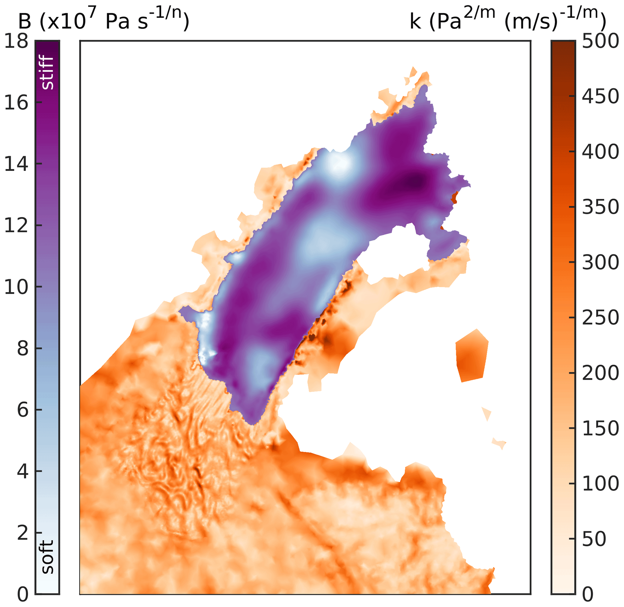
Figure B2 Inferred values for the basal friction coefficient k and the bulk ice rigidity B by the joint inversion.

Figure B3 Surface velocity differences in simulated and observed velocities.

Within the inverse problem a cost function, J, that measures the misfit between observed, $v_{x,y}^{\mathrm{obs}}$, and modelled velocities, v_x,y, is minimized. The cost function is composed of two terms which fit the velocities in fast- and slow-moving areas. A third term is a Tikhonov regularization to avoid oscillations. The cost function is defined as follows:

$$\begin{array}{}\text{(B3)}& {\displaystyle }{J}_{\mathrm{0}}\left(\mathit{v}\right)={\mathit{\gamma }}_{\mathrm{1}}{\displaystyle \frac{\mathrm{1}}{\mathrm{2}}}\underset{d{\mathrm{\Gamma }}_{\mathrm{s}}}{\int }\ln \left({\displaystyle \frac{\sqrt{v_x^{\mathrm{2}}+v_y^{\mathrm{2}}}+\mathit{\epsilon }}{\sqrt{{v_x^{\mathrm{obs}}}^{\mathrm{2}}+{v_y^{\mathrm{obs}}}^{\mathrm{2}}}+\mathit{\epsilon }}}\right)\mathrm{d}{\mathrm{\Gamma }}_{\mathrm{s}},\text{(B4)}& {\displaystyle }{J}_{\text{reg}}\left(B\text{ or }k\right)={\mathit{\gamma }}_{\mathrm{t}}{\displaystyle \frac{\mathrm{1}}{\mathrm{2}}}\underset{{\mathrm{\Gamma }}_{\mathrm{b}}}{\int }\mathrm{\nabla }\left(B\text{ or }k\right)\cdot \mathrm{\nabla }\left(B\text{ or }k\right)\mathrm{d}{\mathrm{\Gamma }}_{\mathrm{b}},\text{(B5)}& {\displaystyle }J(\mathit{v},B\text{ or }k)=J_{\mathrm{0}}\left(\mathit{v}\right)+J_{\text{reg}}\left(B\text{ or }k\right),\end{array}$$

where ε is a minimum velocity used to avoid singularities, and Γ_s and Γ_b are the ice surface and ice base, respectively. An L-curve analysis was performed to pick the Tikhonov parameter γ_t. We obtained excellent agreement with the observed velocities by choosing γ₁=1 and ${\mathit{\gamma }}_{\mathrm{t}}=\mathrm{4}\times {\mathrm{10}}^{-\mathrm{9}}$ (Fig. B3).