Spaceborne thermal infrared observations of Arctic sea ice leads at 30 m resolution

Sea ice leads play an important role in the heat exchange between the ocean and the overlying atmosphere, particularly narrow leads with widths of less than 100 m. We present a method for detecting sea ice leads in the Arctic using high-resolution infrared images from the Thermal Infrared Spectrometer (TIS) on board the Sustainable Development Science Satellite 1 (SDGSAT-1), with a resolution of 30 m in a swath of 300 km. With the spatial resolution of leads observed by infrared remote sensing increasing to tens of meters, focused on the Beaufort Sea cases in April 2022, the TIS-detected leads achieve good agreement with Sentinel-2 visible images. For the three infrared bands of the TIS, the B2 (10.3–11.3 µm) and B3 (11.5–12.5 µm) bands show similar performance in detecting leads. The B1 band (8.0–10.5 µm) can be usefully complementary to the other two bands, as a result of different temperature measurement sensitivity. Combining the detected results from the three TIS bands, the TIS is able to detect more leads with widths less than hundreds of meters compared to the Moderate Resolution Imaging Spectroradiometer (MODIS). Our results demonstrate that SDGSAT-1 TIS data at 30 m resolution can effectively observe previously unresolvable sea ice leads, providing new insight into the contribution of narrow leads to rapid sea ice changes in the Arctic.

1 Introduction

Over several decades, the Arctic has experienced warming at approximately twice the rate of the global average, a phenomenon known as Arctic amplification (Serreze and Francis, 2006) that has attracted increasing attention. Among a suite of causes and processes contributing to Arctic amplification, ongoing changes in the Arctic sea ice extent and the heat fluxes between the ocean and atmosphere are particularly prominent (Serreze and Barry, 2011). Leads are elongated fractures within sea ice that develop as a result of sea ice fracturing under wind and ocean stresses. Although these openings are relatively small, covering less than 2 % of the central Arctic, they hold significant importance for the Arctic mass and heat balance (Vihma et al., 2014). Open water in leads may refreeze when exposed to a cold atmosphere, leaving unfrozen water and ice of varying thicknesses. A small change of 1 % in the lead fraction can cause a large fluctuation in air temperature, up to 3.5 K (Lüpkes et al., 2008). Leads provide windows for heat exchange between the air and water, contributing to over 70 % of upward heat flux (Marcq and Weiss, 2012). During winter, newly opened leads and polynyas are the primary source of ice production, brine rejection, and turbulent heat loss to the atmosphere (Maykut, 1982; Alam and Curry, 1998). In spring, surface melt creates more openings, allowing more heat exchange with the atmosphere (Ledley, 1988; Tschudi et al., 2002). As preferential melting sites in early summer (Alvarez, 2022), leads strongly absorb shortwave radiation during the melting season, promoting lateral and basal melt of sea ice (Maykut, 1982), accelerating sea ice thinning (Kwok, 2018), and decreasing the mechanical strength of sea ice (Gimbert et al., 2012); these processes enable a more considerable drifting speed, deformation, and possibly a faster export (Rampal et al., 2009; Onarheim et al., 2018). In turn, more fracturing and earlier openings are expected to create more intensive networks of leads in the following spring (Steele et al., 2015).

Table 1 Arctic sea ice lead products with their spatial resolutions and time spans.

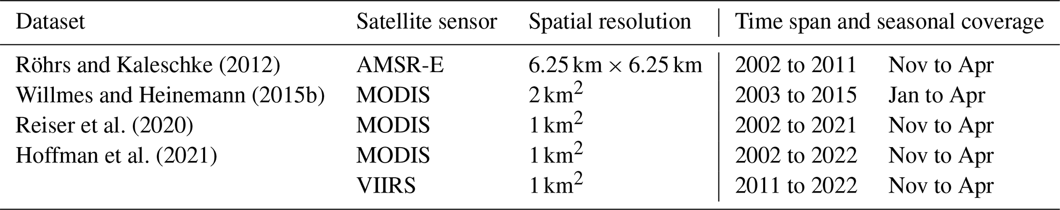
Under the ongoing trend of sea ice retreat in the Arctic (Cavalieri and Parkinson, 2012; Stroeve et al., 2012), identifying the characteristics of sea ice leads can help enhance our understanding of thermodynamic and mechanical processes in the Arctic. Since the early 1990s, various remote sensing instruments, especially by moderate-resolution thermal infrared satellite images, have been used for sea ice lead research, e.g., the Advanced Very High-Resolution Radiometer (AVHRR) (Key et al., 1993; Lindsay and Rothrock, 1995), Moderate Resolution Imaging Spectroradiometer (MODIS) (Willmes and Heinemann, 2015a, b; Hoffman et al., 2019, 2021; Reiser et al., 2020; Qu et al., 2021), Landsat-8 Thermal Infrared Sensor (TIRS) (Wang et al., 2016; Qu et al., 2019; Fan et al., 2020), and FY-3D Moderate Resolution Spectral Imager Type II (MERSI-II) (Wang et al., 2022). High-resolution optical data have also been used for lead detection (Marcq and Weiss, 2012; Muchow et al., 2021). Other studies have applied active and passive microwave data to lead detection, taking advantage of the transparency of microwave wavelengths to cloud cover; however, either the data resolution in these studies is too coarse, e.g., the Advanced Microwave Scanning Radiometer for Earth Observing System (AMSR-E) with a resolution of 6.25 km (Röhrs and Kaleschke, 2012; Bröhan and Kaleschke, 2014), or the observations are discontinuous, e.g., by synthetic aperture radar (SAR) (Murashkin et al., 2018; Murashkin and Spreen, 2019; Liang et al.,2022) and altimeter (Wernecke and Kaleschke, 2015; Lee et al., 2018; Zhong et al., 2023). Table 1 summarizes the publicly available lead datasets, mainly developed based on moderate-resolution thermal infrared, with spatial resolutions on a kilometer scale, limited to the winter season.

The key to detecting sea ice leads using thermal infrared data lies in deriving thermal contrasts, specifically the temperature anomaly between sea ice and open water, and distinguishing leads from thermal contrasts of ice ages and clouds. To this end, previous studies have utilized various temperature datasets. For instance, Willmes and Heinemann (2015a) used the MODIS ice surface temperature (IST) product to map pan-Arctic lead distribution from January to April over the period of 2003 to 2015. They also developed a long-term daily lead product to assess seasonal divergence patterns of sea ice in the Arctic Ocean (Willmes and Heinemann, 2015b). Essentially, IST data, which are usually retrieved using the split-window technique (Key et al., 1997), have challenges in sea ice scenarios with the presence of melt ponds and leads. This is partly due to the lower emissivity (0.96 compared to 0.99) of water compared to sea ice, causing a difference in the retrieved temperature (Jiménez-Muñoz et al., 2014; Fan et al., 2020), especially with mixed-pixel effects (Hall et al., 2001). Moreover, cloud masking defects affect lead detection (Hoffman et al., 2019; Reiser et al., 2020). To address these limitations, Hoffman et al. (2019) focused on using at-sensor brightness temperature (BT) data and improved cloud masking to detect leads for January through April over the period of 2003 to 2018. However, the lead area estimation was lower than that of Willmes and Heinemann (2015b) due to differences in the spatial resolutions of the lead datasets (1 km² compared to 2 km², as listed in Table 1). More recently, Hoffman et al. (2021) applied a convolutional neural network, U-Net, to detect leads based on Visible Infrared Imaging Radiometer Suite (VIIRS) 11 µm BT images (Hoffman et al., 2021). The lead area analysis over the winter season between 2002 to 2022 showed a slight decreasing trend due to increasing cloud cover in the Arctic but an increasing trend of 3700 km² yr⁻¹ after removing the impact of cloud cover changes (Hoffman et al., 2022a). Qu et al. (2021) proposed a modified algorithm from Willmes and Heinemann (2015a) to detect daily spring leads in the Beaufort Sea based on the IST data retrieved from MODIS swath products, providing better results in identifying open water leads and refrozen leads; they found a positive interannual trend in the April lead area for the study period of 2001 to 2020 of approximately 2612 km² yr⁻¹.

Accurate lead observations are crucial to understanding rapid sea ice changes in the Arctic Ocean (Zhang et al., 2018; Ólason et al., 2021). Narrow leads of less than a 100 m in width are over 2 times more efficient at transmitting turbulent heat than larger leads of hundreds of meters (Marcq and Weiss, 2012). However, due to the limitations of spaceborne thermal infrared sensors in terms of spatial resolution, current lead observations are only available at a moderate resolution on a kilometer scale. Key et al. (1994) assessed the effect of sensor resolution on lead width statistics and suggested that the mean lead width expands as the pixel size builds up in gradually degraded images. Qu et al. (2019) resampled Landsat-8 TIRS data with a resolution of 100 to 30 m to estimate heat fluxes over the detected leads. Their result showed underestimated lead information detected by MODIS data compared to TIRS data. Consequently, the heat flux estimation from Landsat-8 TIRS data is larger than that from MODIS data, where small leads contribute to more than a quarter of the total heat flux. Yin et al. (2021) proposed a convolutional-neural-network-based framework to estimate turbulent heat flux over leads at the sub-pixel scale using MODIS data. The super-resolution estimates are better than those obtained from the original moderate-resolution data (1 km) and interpolation-based high-resolution data (100 m) but still have limitations for very narrow leads. Consequently, the kilometer-scale spatial resolution is inadequate for reproducing the actual lead characteristics in the Arctic Ocean. High-resolution observations are essential for revealing narrow leads and their dynamics.

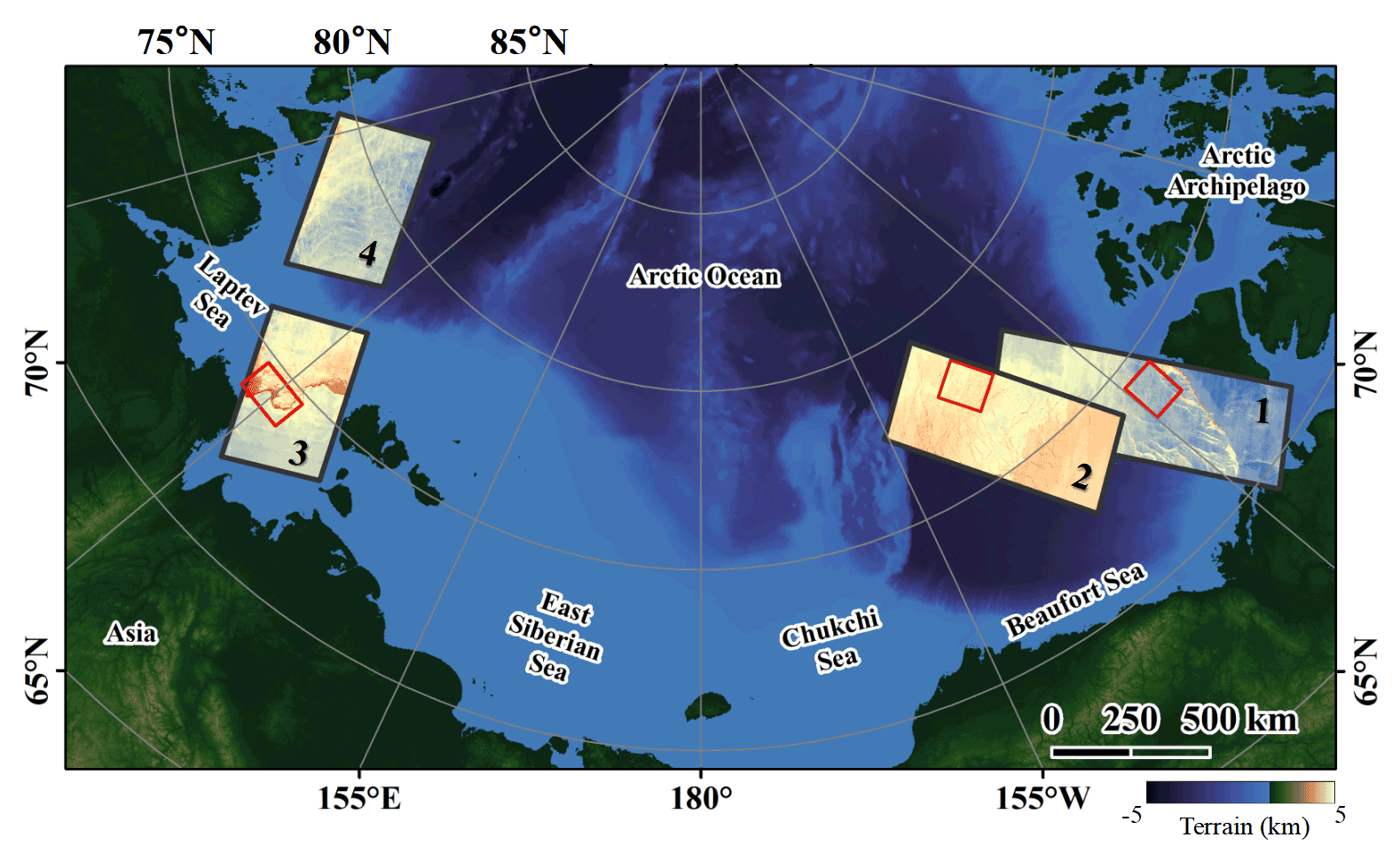
Figure 1 Geospatial distributions of SDGSAT-1 TIS data collected from the Arctic Ocean in March and April 2022 used in this study for sea ice lead detection. The black borders mark four successive groups of cloudless images (group 1 was acquired on 3 April, group 2 on 28 April, and groups 3 and 4 on 23 March), with color representing the BT values from the TIS B2 band. The small red squares indicate regions where the TIS data are matched with Sentinel-2 visible images for validation.

An emerging opportunity to obtain high-resolution observations is the Sustainable Development Science Satellite 1 (SDGSAT-1), which was successfully launched on 5 November 2021 and is the first satellite customized for the United Nations (UN) 2030 Agenda for Sustainable Development (Guo et al., 2021). Three payloads, the thermal infrared spectrometer (TIS), glimmer imager, and multispectral imager, allow the satellite to obtain high-quality data, as well as full-time monitoring capabilities to facilitate the evaluation of Sustainable Development Goals (SDGs) (Guo et al., 2022). The TIS is used for global thermal radiation detection with three thermal infrared bands (see Sect. 2.1 for data details). More importantly, the TIS has a spatial resolution of 30 m, with a wide swath of 300 km. With such an unprecedented infrared imaging capability, SDGSAT-1 TIS is expected to provide far more details of sea ice characteristics in polar regions than current thermal infrared sensors in orbit. To date, the TIS has acquired substantial high-resolution thermal infrared data from the critical seas in the Arctic, including the Beaufort Sea and the Laptev Sea, which are pervaded by leads with significant sea ice dynamic processes (Wernecke and Kaleschke, 2015). Figure 1 presents a few cases in March and April 2022 under clear-sky conditions. Under such attractive prospects, we pioneered the scientific application of SDGSAT-1 TIS data to examine its feasibility in detecting sea ice leads from the Arctic Ocean. With regard to the thermal characteristics of high-resolution data, we proposed an improved lead detection method based on a combination of binary segmentation and a designed filter. To determine the reliability of the detailed features resolved at 30 m resolution, a series of comparisons were performed, including comparisons with visible and SAR data at high resolutions, as well as comparisons with comparable lead products at moderate resolutions.

This study focuses on observing Arctic sea ice leads based on spaceborne thermal infrared remote sensing at 30 m resolution and reveals more details than the moderate-resolution thermal infrared sensor. The results will help us to understand the processes of Arctic lead variability and its contribution to Arctic sea ice retreat. The paper is organized as follows. Section 2 introduces the data used in this study, including SDGSAT-1 TIS data for lead detection, visible images for validation, and others for comparative analysis. Section 3 presents the method applied to derive sea ice leads. Section 4 presents the high-resolution lead detection results of this study, the validation against visible images, the cross-comparison among three infrared bands, and the comparison with the moderate-resolution results. In Sect. 5, we explore the factors affecting lead detection and the lead properties resolved by high-resolution imagery. Finally, a summary and conclusion are given in Sect. 6.

2 Data and pre-processing

2.1 SDGSAT-1 TIS

As listed in Table 2, the TIS has three infrared bands, which are centered at 9.3 µm (8.0–10.5 µm; band 1, B1), 10.8 µm (10.3–11.3 µm; band 2, B2), and 11.8 µm (11.5–12.5 µm; band 3, B3) with a resolution of 30 m in a swath of 300 km (and the ground segment crops the original TIS data to 300 km in the along-track dimension for convenient use), and it has the ability to detect temperature differences with an accuracy of NEDT (noise equivalent differential temperature) less than 0.041 K at 300 K (Guo et al., 2022). In the commissioning phase of the satellite, the analysis shows that the accuracy of the radiometric measurement is better than 0.661, 1.081, and 0.426 K for B1, B2, and B3 bands (Y. Hu et al., 2022), satisfying the preflight requirements (≤ 1 K). In particular, the B1 band shows less strip noise (i.e., signal fluctuations along the sensor scan caused by detector noise) than the other two bands. The B2 and B3 bands are widely used in surface temperature retrieval as two split-window channels, while the B1 band is not commonly used in infrared observation missions. As a wide channel with a wavelength of 8.0–10.5 µm, the B1 band is commonly used in conjunction with the B2 and B3 bands with the aim of improving the precision of surface temperature retrieval based on the three-channel split-window algorithm (Liu et al., 2021; Z. Hu et al., 2022). Liu et al. (2021) estimated the ability of SDGSAT-1 TIS data to retrieve land surface temperature when different split-window algorithms were applied, i.e., the generalized split-window algorithm using the B2 and B3 bands and the three-band split-window algorithm using the B1, B2, and B3 bands together. Their results showed that the three-band method performs better than the two-band method with a root mean square error lower than 1 K.

Table 2 SDGSAT-1 TIS characteristics and radiometric performance (CBAS, 2022).

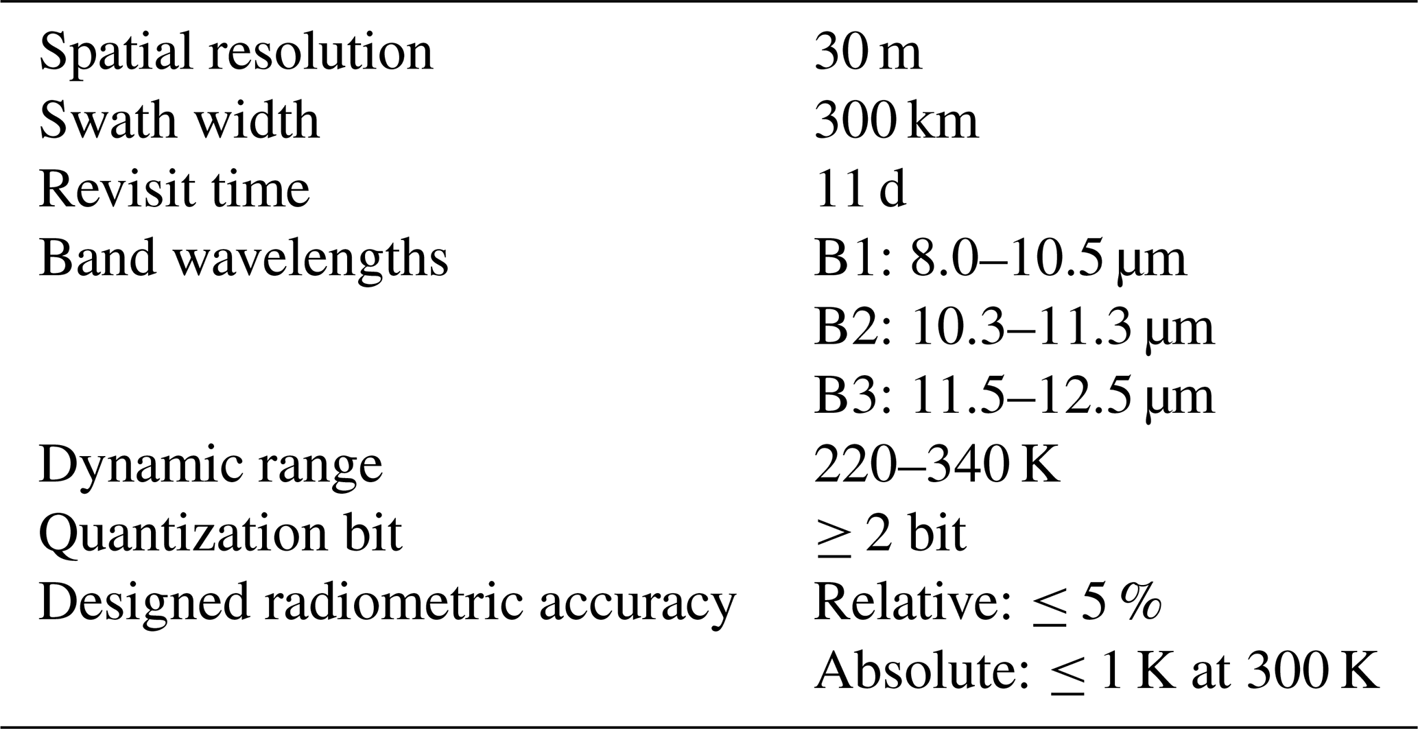
Table 3 Information on satellite data and derived products used in this study.

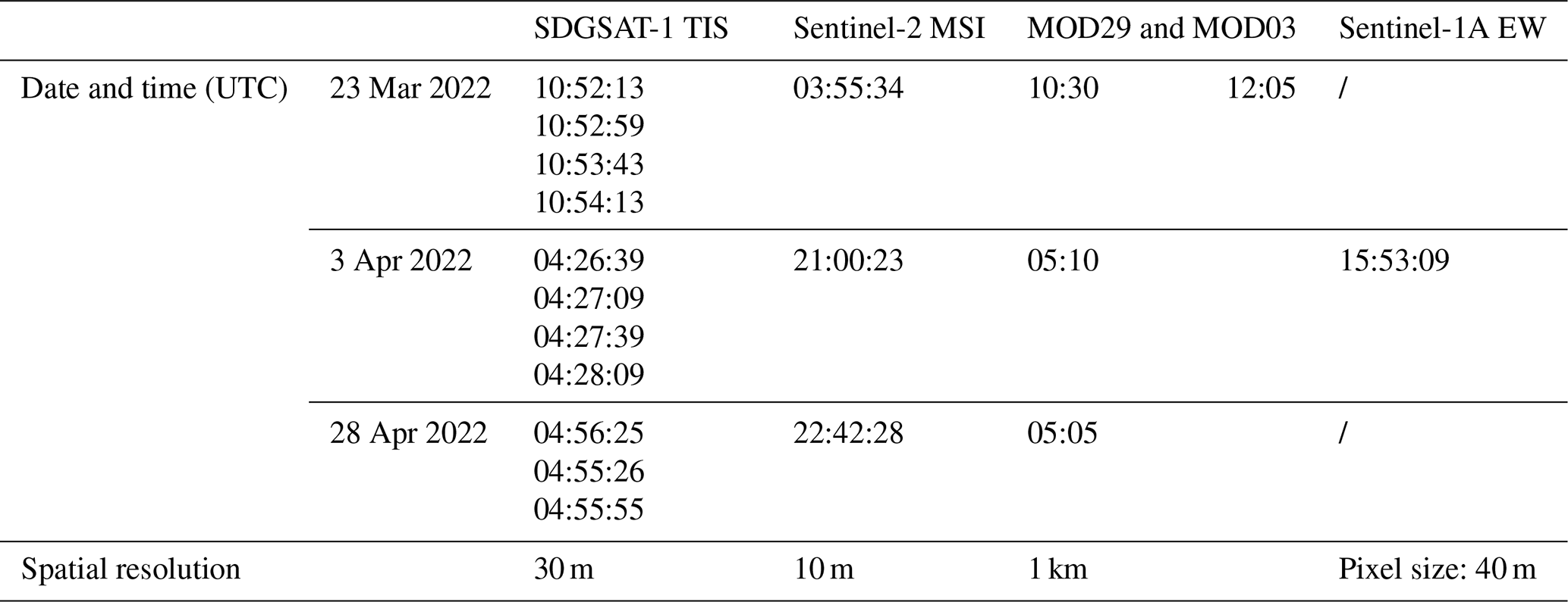
Considering the benefit of incorporating three thermal infrared bands for observation, all three bands of SDGSAT-1 TIS are used for lead detection in this study. The georeferenced level-4 TIS data are based on the level-1 product after ortho-rectification using ground control points, a digital elevation model (DEM), and output with a standardized format (CBAS, 2022). Since SDGSAT-1 was launched in November 2021, the development of TIS-based surface temperature products or cloud mask products is currently under development. We collected the TIS data from the Beaufort Sea and the Laptev Sea during the spring season of 2022 and manually selected the data with cloud coverage of less than 10 % for sea ice lead detection. Considering diverse imaging requirements across various domains, it poses a challenge for SDGSAT-1 to maintain prolonged surveillance of polar regions. The set of 11 TIS images, presented in Fig. 1 and composed of four consecutive scenes, encompasses the majority of the available data up until the time of writing, and the corresponding information is provided in Table 3.

All digital numbers (DNs) are converted into at-sensor radiance using Eq. (1).

$$\begin{array}{}\text{(1)}& L=\mathrm{gain}\times \mathrm{DN}+\mathrm{bias}-\mathrm{bg},\end{array}$$

where the gain and bias are radiometric calibration coefficients provided by the scientific calibration team, which have included relative and absolute radiometric calibrations, and bg is the background radiance of the black body. Then, the BT is calculated from the at-sensor radiance using the Planck function.

2.2 Sentinel-1 and Sentinel-2

Sentinel-2 (S2) is a constellation of two satellites, S2A and S2B, both equipped with a Multispectral Instrument (MSI) with 13 spectral channels covering the visible, near-infrared, and shortwave-infrared spectral zones (ESA, 2022b). Level-1c S2 products provide top-of-atmosphere reflectance processed with radiometric and geometric corrections in tile form, with each tile being an orthoimage in a 100 km by 100 km area. S2 MSI visible images at a resolution of 10 m are used to compare with the leads detected by the TIS in this study for validation. We mainly used the band 3 (560 nm) data, which offers good discrimination between leads and surrounding sea ice in visual comparisons for the scenarios applied in this study. Images acquired over the Beaufort Sea and the Laptev Sea in March and April 2022 were collected (see Table 3 for the data information and the red squares in Fig. 1 for their coverage).

Sentinel-1 (S1) is a C-band SAR that operates day and night regardless of the weather. Both S1A and S1B acquire dual-polarization (HH and HV) imagery, covering the vast Arctic region. The S1 Extra Wide (EW) swath data have a swath width of approximately 400 km, with a pixel size of 40 m by 40 m (ESA, 2022a). We used the S1 level-1b data in the format of ground range detected medium resolution (GRDM). As S1B has been out of operation since December 2021, only the S1A data are available during this study period. Considering that the backscatter values of SAR in different polarizations give different sensitivities for fully open leads or leads covered by thin ice, we collected S1A dual-polarization data in the Beaufort Sea on 3 April 2022 (see Table 3). The dual-polarization data were radiometrically calibrated, and a false-color composition was performed by assigning the HH, the subtraction of HH from HV, and the HV images to the red, green, and blue channels, respectively.

2.3 MODIS products

MODIS is an instrument on board the two polar-orbiting satellites, Terra and Aqua, which are part of NASA's Earth Observing System (EOS). MODIS acquires data in 36 discrete spectral bands that cover the optical to thermal infrared radiance wavelength region. The swath width of MODIS is 2330 km. The daily level-2 sea ice products, MOD29 and MYD29, include sea ice cover and IST datasets (Hall and Riggs, 2021). Each product contains 5 min of swath data observed at a resolution of 1 km. The IST data are retrieved using the split-window technique based on the MODIS 31 and 32 bands, with an accuracy of 1.2–1.3 K (Hall et al., 2004). Cloud masking from the MODIS cloud products for daytime and nighttime (Ackerman et al., 1998) is integrated into the IST retrieval. The IST data produced by MODIS/Terra, i.e., MOD29 products and the MOD03 geolocation product (MODIS Characterization Support Team, 2017), are used in this study (see Table 3 for data information).

2.4 ERA5 air temperature data

The European Centre for Medium-Range Weather Forecasts (ECMWF) provides the fifth-generation reanalysis data (ERA5) for global climate and weather for the past seven decades (Hersbach et al., 2018). The ERA5 near-surface air temperature (2 m air temperature) data are available hourly in a regular grid of 0.25^∘. In this study, we used 2 m air temperature data for the period between March and April 2022 to explore the possible variations in the atmospheric environment.

2.5 OMI/Aura product

Since the TIS B1 band (8.0–10.5 µm) corresponds to an absorption channel for ozone (Wan and Li, 1997), we analyzed the potential absorption effects of different ozone solutions on thermal infrared radiation in this study. The Ozone Monitoring Instrument (OMI) is an instrument on board the EOS Aura mission. The OMI measurements cover a spectral region of 264–504 nm, which aims to continue the record for total ozone and other atmospheric parameters related to ozone chemistry and climate. The total column ozone is retrieved based on the long-standing TOMS V8 retrieval algorithm (Bhartia, 2002), which uses a weakly absorbing wavelength (331.2 nm) to estimate an effective surface reflectivity and another wavelength (317.5 nm) with stronger ozone absorption to estimate ozone. The level-3 OMI/Aura Ozone Total Column (OMTO3) data are produced using best pixel data from approximately 15 orbits, covering the whole globe and mapped in a grid size of 0.25^∘ (Bhartia, 2012).

3 Method

In this section, we propose a method for sea ice lead detection adaptable to high-resolution TIS images based on the principle of exploiting both the relative and absolute temperature characteristics of sea ice leads.

Leads containing seawater and thin ice have temperatures higher than the surrounding sea ice. Therefore, detecting leads is based on the temperature contrast between leads and the sea ice surface (Willmes and Heinemann, 2015a; Hoffman et al., 2019; Qu et al., 2021). However, as the spatial resolution of thermal infrared imagery improves, the temperature variations in sea ice with different thicknesses pose a challenge for accurate lead identification. To address this issue, the algorithm we proposed mainly involves two steps: a segmentation and a filter, which correspond to the two major steps in the flowchart in Fig. 2. The algorithm's input is the BT data of each TIS band (B1, B2, and B3 bands). A representative scenario containing both large and narrow leads, along with surface temperature variations, is presented in Fig. 3a, using the TIS B1 band as an example. Thanks to the high spatial resolution of 30 m, the thermal features of sea ice and leads are clearly observable. In addition to the leads presenting as distinct yellow and red colors (in the temperature range of 242 to 252 K) on the BT map, slight variations in sea ice surface temperature can be identified from approximately 237 to 242 K. The brightness temperature anomaly (BTA) images are derived from the BT data by subtracting the mean temperature in neighboring windows with sizes of 2.4 km by 2.4 km (80 pixels by 80 pixels), as shown in Fig. 3b. Undoubtedly, the BTA data further highlight the presence of leads, but the positive BTA values caused by thinner sea ice are also highlighted. To this end, the first step of our lead detection involves applying a binary segmentation to extract potential leads from the BTA data. In the second step, the derived potential leads are used together with the BT data to extract the BT values of the potential leads and then used in a designed filter to obtain the consequent leads. The next two subsections describe the two major steps involved in the proposed method.

Figure 2 Flowchart of sea ice lead detection based on SDGSAT-1 TIS data.

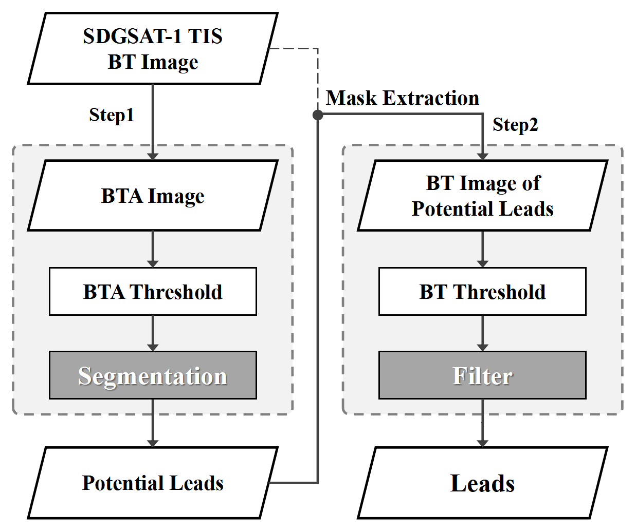
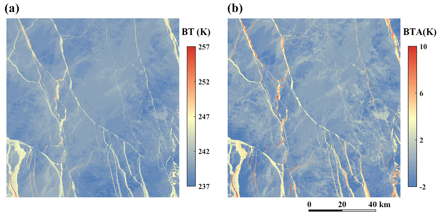
Figure 3 Example for the BT image and BTA image based on the SDGSAT-1 TIS B1 band (8–10.5 µm) acquired on 3 April 2022. (a) The BT image. (b) The derived BTA image. SDGSAT-1 TIS data ID: KX10_TIS_20220403_W128.84_N73.00_202200033226.

3.1 Potential lead segmentation based on BTA data

The key to performing a binary segmentation of the BTA data is to identify an appropriate threshold to segment sea ice and leads. To achieve this, we collected seven TIS data acquired between 3 and 28 April 2022 in the Arctic Ocean and analyzed the distribution of their BTA data, as illustrated in Fig. 4. The BTA data follow a normal distribution, as demonstrated by the Gaussian fitting (with μ = −0.25 K, σ² = 0.38 K) overlaid on the graph. The histogram displays a peak at −0.25 K, accounting for 15.09 % of all the data. The long tail on the positive side of the histogram suggests the presence of leads in the images, as they have higher temperatures than the surrounding ice. Therefore, it is necessary to determine a threshold in the positive BTA range to accurately segment the leads from other features.

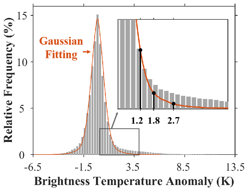
Figure 4 Statistical BTA histogram of seven TIS data acquired from 3 April to 28 April 2022 with a bin width of 0.25 K. The orange curve is the Gaussian fitting, with μ = −0.25 K and σ² = 0.38 K.

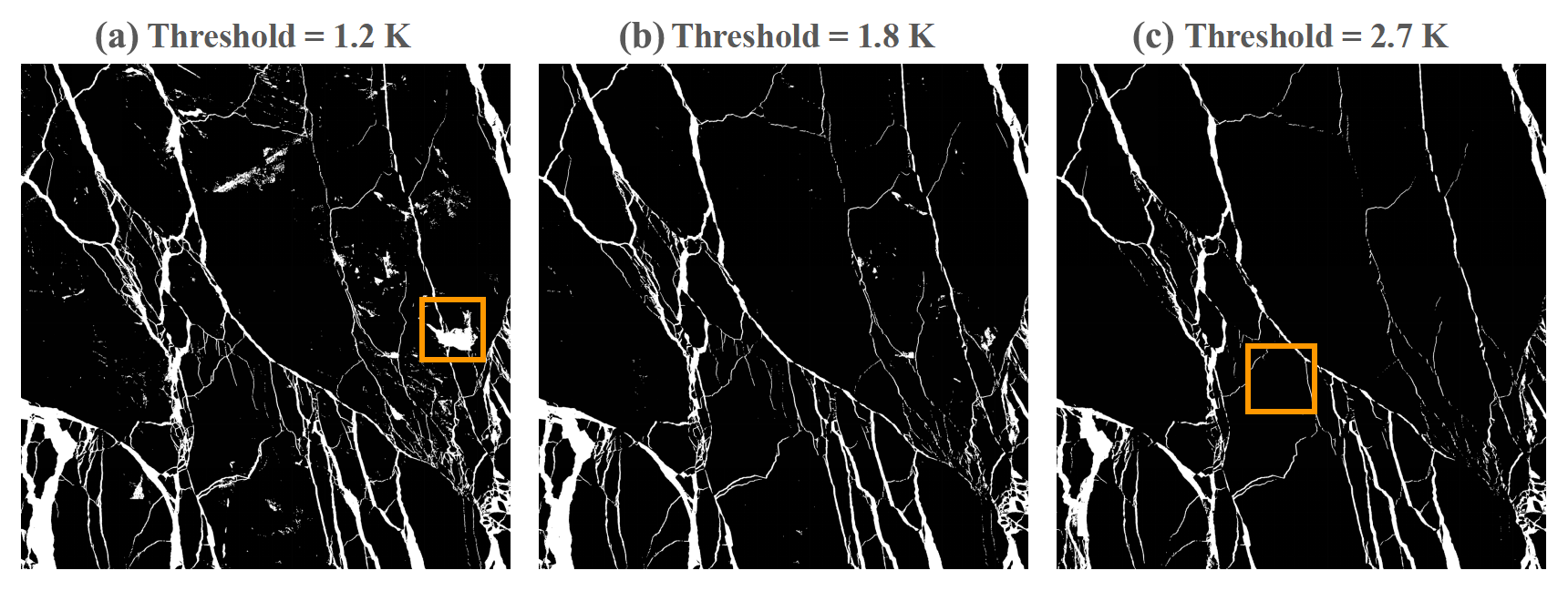
Figure 5 BTA threshold tests for potential lead segmentation using the thresholds of (a) 1.2, (b) 1.8, and (c) 2.7 K. BTA values greater than or equal to the threshold are classified as 1 (white areas), and values less than the threshold are assigned 0 (black background). Orange squares indicate false detections. SDGSAT-1 TIS data ID: KX10_TIS_20220403_W128.84_N73.00_202200033226.

Previous studies applied various BTA thresholds for lead detection (Willmes and Heinemann, 2015a; Hoffman et al., 2019; Qu et al., 2021). For instance, based on BTA data derived from the MODIS IST product, Willmes and Heinemann (2015a) compared the standard deviation and non-parameterized methods. In terms of BTA data derived by MODIS 11 µm swath data, Hoffman et al. (2019) identified a threshold of 1.5 K. Qu et al. (2021) took 1.2, 1.5, and 2 K as thresholds for different types of leads, corresponding to large to small uncertainty levels. We enlarged a part of the histogram tail in Fig. 4 and observed that the Gaussian curve gradually deviates from the bars when the BTA value exceeds 1.2 K, indicating a transition from ice to leads. We tested various thresholds and found that selecting 1.2, 1.8, and 2.7 K as thresholds results in distinguishable differences in the segmentation results, as illustrated in Fig. 5. Using a threshold of 1.2 K results in false-positive detections (i.e., sea ice or other features classified as leads), as exemplified by the white pixels marked by the orange square in Fig. 5a (this can be identified in the original BTA map shown in Fig. 3b). In contrast, using 2.7 K as the threshold causes a loss of detail, as highlighted by the part marked by the orange square in Fig. 5c (compared to Fig. 5b). Multiple threshold segmentation was tested by varying the BTA threshold from 1.2 to 2.7 K in 0.1 K steps. After visual comparison, we found that using 1.8 K as the threshold yields a significantly different segmentation effect, which avoids many false-positive detections while still capturing lead details, as demonstrated in Fig. 5b. Apart from the fixed thresholds, we have also assessed the thresholds selected through an iterative method (Willmes and Heinemann, 2015a) which produced similar outcomes to the manually selected fixed threshold of 1.8 K. Therefore, a BTA threshold of 1.8 K was applied to all SDGSAT-1 TIS data in this study for potential lead segmentation.

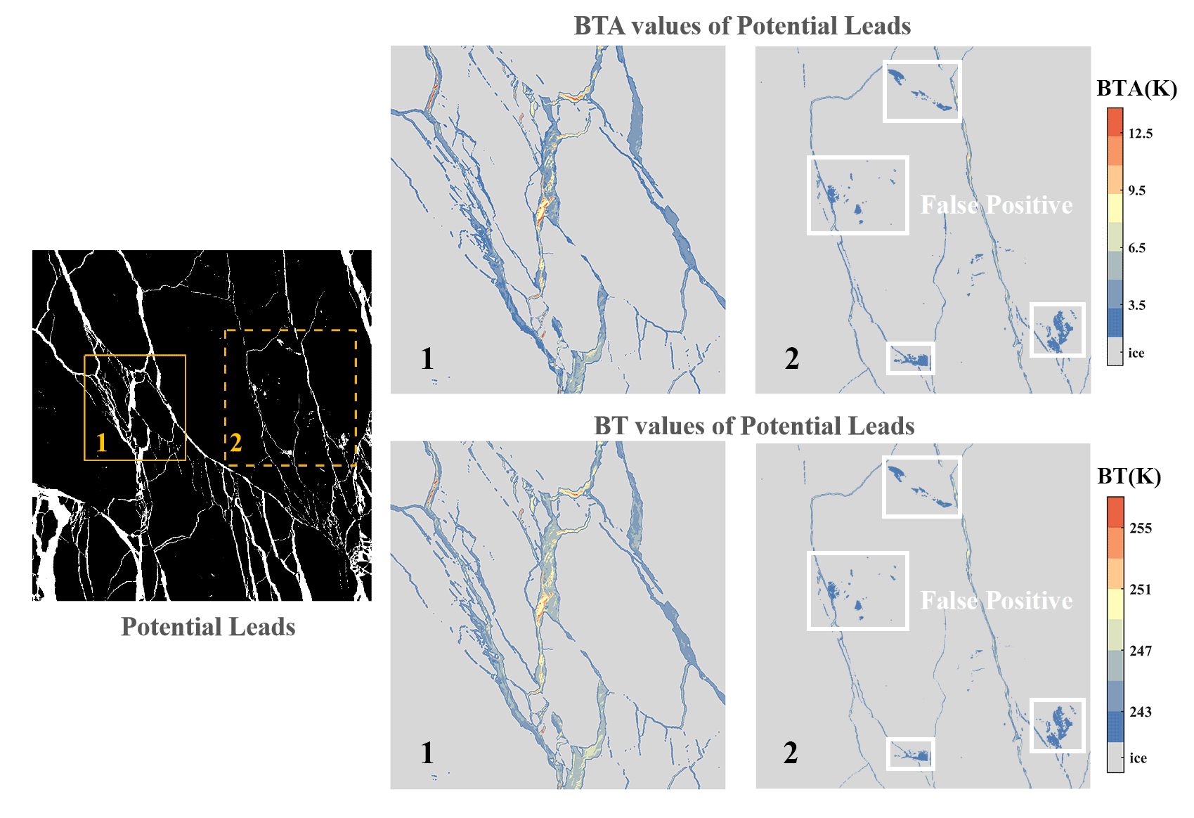
Figure 6 Characteristics of potential leads after segmentation. The left panel presents a binary image of potential leads detected by segmentation (the same as Fig. 5b), with the two squares highlighted: view 1 represents highly reliable detection, while view 2 is part of false-positive detection. Corresponding to the two views, the right panel displays the BTA images of these potential leads in the first row and the BT images in the last row, with the gray background representing the ice surface. SDGSAT-1 TIS data ID: KX10_TIS_20220403_W128.84_N73.00_202200033226.

3.2 Further filter based on a BT threshold

After conducting the segmentation in the previous step, a few false-positive detections remain in the result. False-positive detections can be attributed to imperfectly removed clouds, cloud edges, or sea ice of different thicknesses. These interferences cause gradient variations in the BT values measured by the TIS sensor, resulting in high BTA values. To improve the detection accuracy, we decided to identify the reliability of those potential leads. In the left panel of Fig. 6, the potential leads within the square marked by solid yellow lines (in view 1) are considered reliable, while parts of the white pixels marked by the other square with dashed lines (in view 2) are false-positive detections. The right parallel panels of Fig. 6 show the BTA and BT data of the potential leads for the two views. Whether for the first-row BTA or second-row BT data, the dark blue pixels (marked by white squares) are more likely to represent false-positive detections. However, it is difficult to evaluate further the reliability of potential leads based only on the BTA data, as both views in the first row have BTA values close to dark blue with no significant differences. In contrast, false-positive detections could be easily distinguished from leads based on the BT data. For example, in the second row of right parallel panels, the absolute values of the BT of reliable leads in the first column (view 1) are all greater than those of the false-positive detections in the second column (view 2) by at least 2 K.

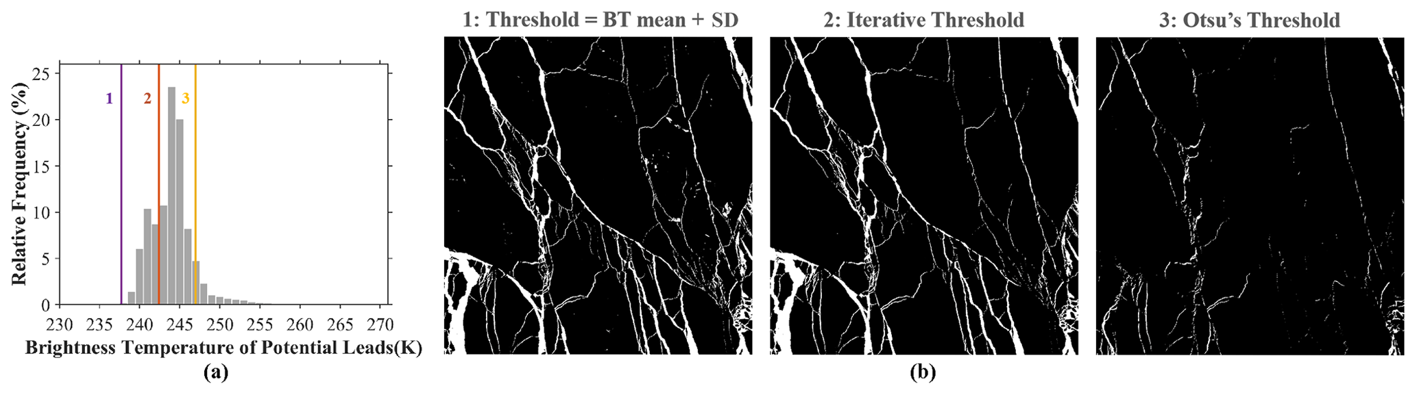
Figure 7 BT threshold tests and filtered results by different thresholds: 1 – mean plus standard deviation (SD) of BT before segmentation; 2 – iterative threshold; and 3 – Otsu's threshold. (a) BT histogram of potential leads, with the overlaid three lines indicating the three BT thresholds selected for the filter. (b) The filtered results of the three thresholds, where the pixels with BT values below the threshold are rejected and classified as background. SDGSAT-1 TIS data ID: KX10_TIS_20220403_W128.84_N73.00_202200033226.

The BT histogram for the potential leads is shown in Fig. 7a. The pixels with low temperature on the left side represent the false-positive detections; the high-frequency pixels and the tail on the right represent highly reliable leads. Thus, we used a filter to remove the pixels with BT values below a given threshold. Unlike the BTA threshold as a constant, the threshold determined for the BT data is adaptive for environmental variations. In this regard, we tested non-parameterized threshold selection methods, including Otsu's threshold (Otsu, 1979), iterative selection (Ridler and Calvard, 1978), and the threshold based on the BT mean and standard deviation (calculated by the BT map before segmentation). The selected thresholds are shown as the three lines in Fig. 7a, and the filtering results using these thresholds in Fig. 7b suggest that the iterative threshold filter performs the best in rejecting false detections. The mean and standard deviation filter ranks second. Otsu's threshold is not adapted for this filter. Therefore, we chose the iterative selection as the method to determine the BT threshold in this filter. The starting position of the iteration is set to the sum of the BT mean and standard deviation, which can save iterative times. For each TIS band, the respective threshold was selected, and the pixels with BT values below the threshold were filtered out. Finally, three binary results at 30 m resolution were derived separately from each of the three bands of the SDGSAT-1 TIS.

4 Results

This section presents the derived sea ice leads at a 30 m resolution based on SDGSAT-1 TIS data in the Arctic Ocean and detailed comparisons with the S2 data and with the MODIS-derived leads, as well as the cross-comparisons among the three bands. The results are based on a total of 11 TIS data that are grouped into four scenes and have three sub-regions for the matching comparison with the S2 (see Fig. 1).

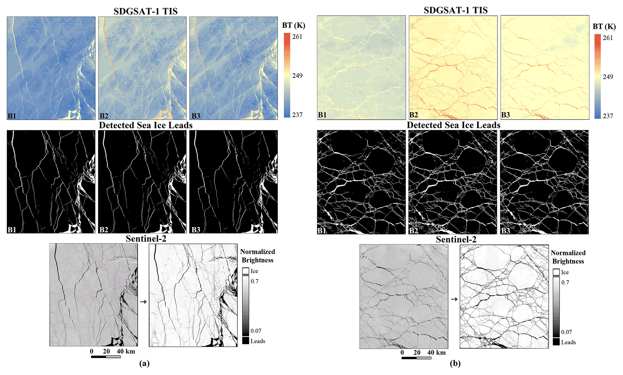
Figure 8 Validation of sea ice lead detection based on SDGSAT-1TIS data compared with S2 visible images of the Beaufort Sea in April 2022. Rows show the BT maps for the B1, B2, and B3 bands, the lead detection results, the S2 band 3 (560 nm) images, and the normalized brightness (from 0.07 to 0.7). (a) TIS data acquired at 04:28 UTC and S2 data at 21:00 UTC on 3 April 2022. IDs: KX10_TIS_20220403_W128.84_N73.00_202200033226 and KX10_TIS_20220403_W132.14_N74.67_202200033227. (b) TIS data acquired at 04:56 UTC and S2 data acquired at 22:42 UTC on 28 April 2022. ID: KX10_TIS_20220428_W147.26_N77.60_202200049406.

Table 4 Definition of the comparison result of the binary lead detection with the visible images with normalized brightness.

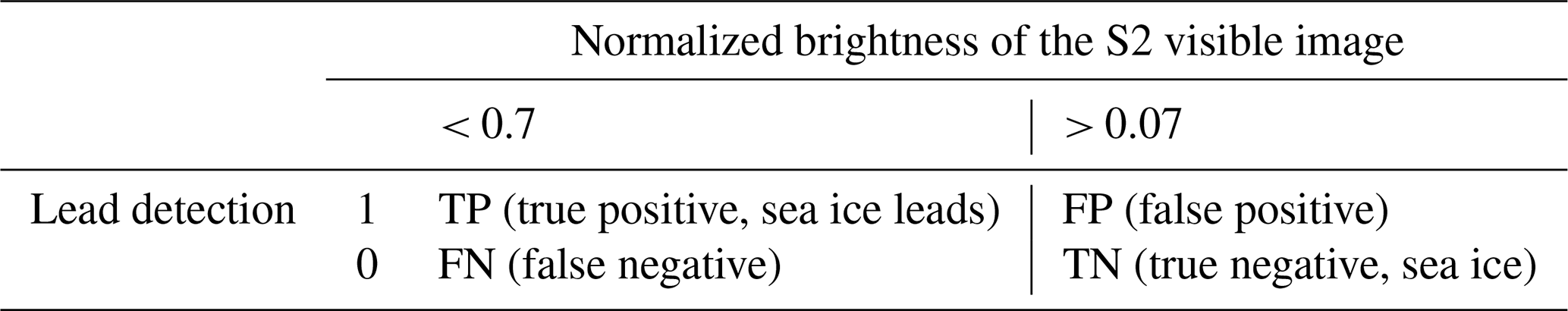
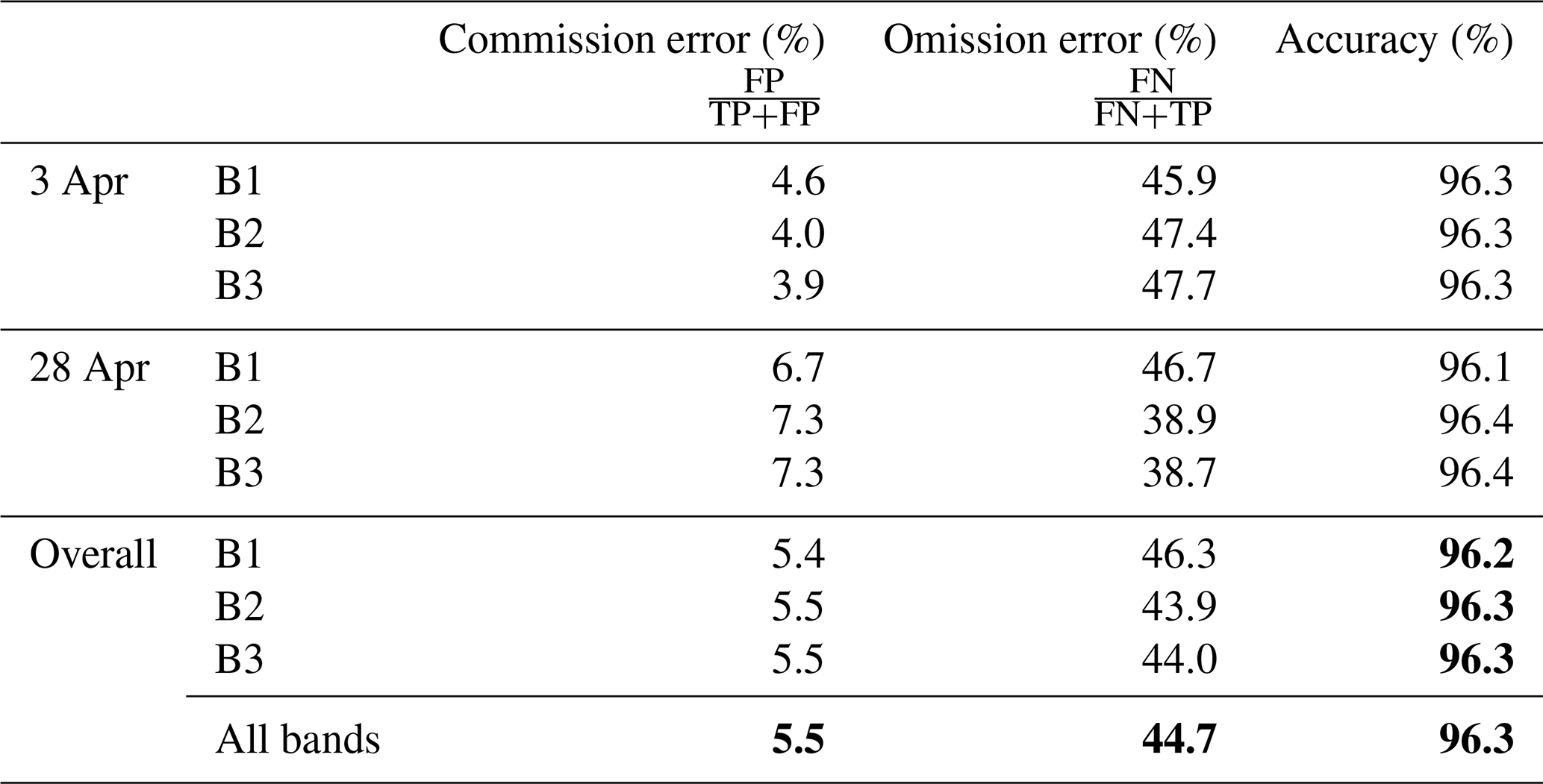
Table 5 Lead detection performance based on the TIS data in the Beaufort Sea on 3 and 28 April 2022. Results from each TIS band are aggregated into overall results (bold in the last column), which are then aggregated into the all-band results (bold in the last row).

4.1 Comparison of TIS-detected sea ice leads with Sentinel-2 images

To assess the reliability of sea ice leads detected in this study, we conducted a comparison of typical cases under clear-sky conditions. Two cases in the Beaufort Sea near the Canadian Arctic Archipelago are presented, as sea ice leads in this region exhibit typical seasonal variations (Steele et al., 2015). Here, we focused on the leads detected in April 2022 (marked by red squares on borders 1 and 2 in Fig. 1) and validated them using co-located S2 MSI visible images. The first row of Fig. 8 displays the three BT maps, with the detected leads represented by the white pixels in the binary maps that follow. For the matched visible images, leads are darker than the ice surface. According to a previous study based on leads using S2 data (Muchow et al., 2021), we calculated the normalized brightness and determined that a pixel with a normalized brightness below 0.7 could be a lead, while a pixel with a normalized brightness above 0.07 could be sea ice. Pixels with normalized brightness between 0.07 and 0.7 are considered to have both possibilities. Apparently, our detection results based on the three infrared bands are highly consistent with these visible images. In particular, it is likely that some of the narrow leads we detected, with widths of tens of meters, have just formed, which are also subtle in 10 m resolution visible images.

We performed a pixel-by-pixel comparison between the TIS-based leads and visible images. Table 4 lists the definitions of TP (true positive), FP (false positive), FN (false negative), and TN (true negative) used in this study. Due to the imbalance between the distribution of leads and the ice background, we used three indicators to evaluate the detection performance: commission error, omission error, and accuracy. The statistics listed in Table 5 for the two cases in the Beaufort Sea show that, for all bands, the commission error, omission error, and accuracy are 5.5 %, 44.7 %, and 96.3 %, respectively. The overall accuracy for the three bands achieves a high level of 96.2 %, 96.3 %, and 96.3 %, respectively. The B1 band shows satisfactory results with an overall commission error of 5.4 % but yields a slightly high miss rate of 46.3 %. The omission error is mainly attributed to a large FN result, resulting from refrozen leads covered by thin ice. More specifically, the case on 3 April (shown in Fig. 8a) yields a commission error of less than 4.6 %, while the commission error on 28 April is slightly higher than the former. The reason lies in the differences in the lead distribution. For the case of 28 April (shown in Fig. 8b), more leads undoubtedly exacerbate the difficulty in detection.

Moreover, the BT values recorded by SDGSAT-1 TIS on these 2 d were different. Even in the overlapping region of borders 1 and 2 in Fig. 1, the BT on 28 April is approximately 5 K higher than that on 3 April. This finding may imply a short-term temperature variation in the late spring, allowing for the formation of more leads and exhibiting more intricate lead networks. On the other hand, a warming environment can reduce the contrast in thermal infrared data, resulting in lower BTA values for leads. The phenomenon is related to different atmospheric conditions, which we further analyze in the Discussion.

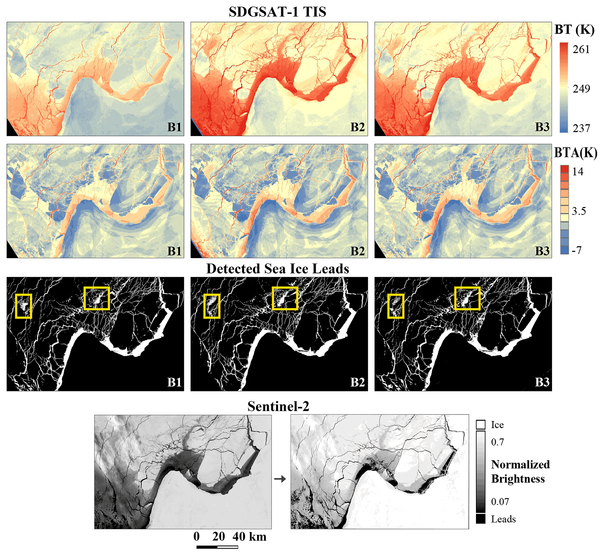
Figure 9 Application of the lead detection method to the SDGSAT-1 TIS data acquired over the Laptev Sea at 10:53 UTC on 23 March 2022 and comparison with the S2 visible image at 03:55 UTC on the same day (similar illustration to the previous figure). IDs: KX10_TIS_20220323_E129.38_N75.60_202200028841 and KX10_TIS_20220323_E133.08_N73.96_202200028843.

Applying this detection method to the TIS data acquired over the Laptev Sea on 23 March 2022 (shown within rectangle 3 in Fig. 1), we found a complex situation when compared to the S2 visible image, as shown in Fig. 9. The expansive gray feature in the S2 images is more likely to be cloud shadow than leads (McIntire and Simpson, 2002). Detecting leads under this interference is quite challenging since the thermal contrast is far less distinct than that on a clean ice surface, as shown in the following BTA maps. Compared to the visible image, the accuracy values for the B1, B2, and B3 bands are 95.5 %, 95.4 %, and 95.6 %, respectively. However, some FP detections remain in the three bands, which are marked by yellow rectangles in the third row. Thus, although this detection based on SDGSAT-1 TIS data shows promising applicability, the uncertainty caused by cloud interference remains to be further explored.

4.2 Cross-comparison of sea ice lead detection based on the three TIS infrared bands

The three TIS bands all yield good accuracy in lead detection but do present some discrepancies. In this subsection, we performed cross-comparisons of these results to focus on the effectiveness of the three thermal infrared bands in detecting leads. Counting the lead pixels derived from each TIS band, a total of 46 301 986 pixels comprise the consistency detection (co), i.e., a pixel that is detected as a lead in all three bands. Thus, the additional detection (ad) is calculated (i.e., detected as a lead by a specific band) using Eqs. (2) and (3).

$$\begin{array}{}\text{(2)}& {\displaystyle }{N}_{\mathrm{Bn},\mathrm{ad}}=N_{\mathrm{Bn}}-N_{\mathrm{co}},\text{(3)}& {\displaystyle }{P}_{\mathrm{Bn},\mathrm{ad}}=N_{\mathrm{Bn},\mathrm{ad}}/N_{\mathrm{co}}\times \mathrm{100}\mathit{\%},\end{array}$$

where N is the total number of pixels, Bn is the infrared band (n = 1, 2, 3), and P is the proportion. The results listed in Table 6 show that the additional detections from the B1, B2, and B3 bands account for 11.46 %, 23.30 %, and 21.88 %, respectively. The fewest leads are detected by the B1 band, while the B2 and B3 bands give similar results.

Table 6 Statistics of lead pixels detected based on the three infrared bands of the SDGSAT-1 TIS.

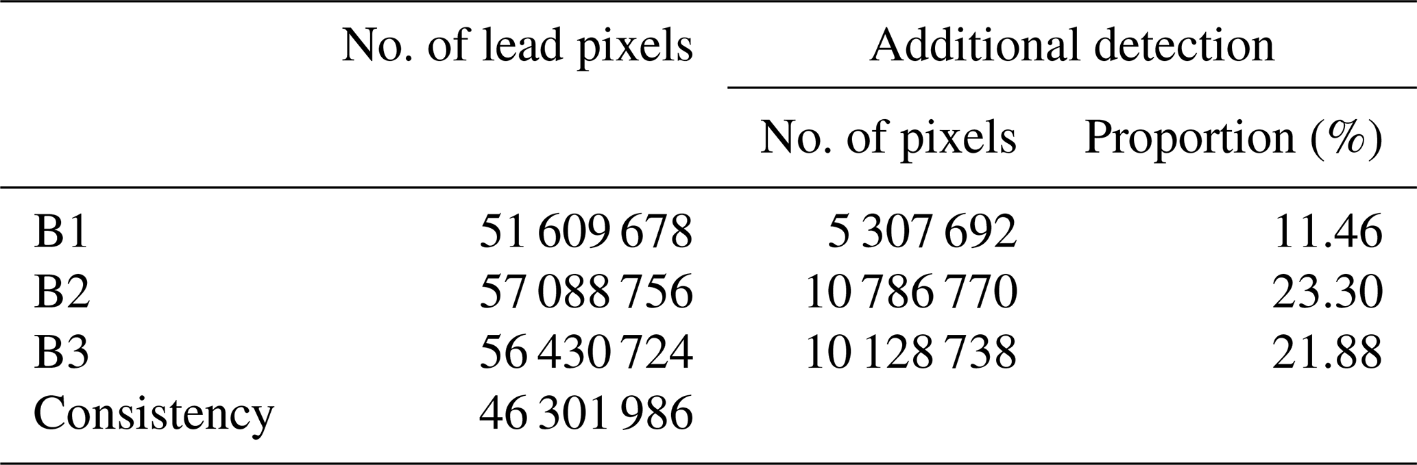
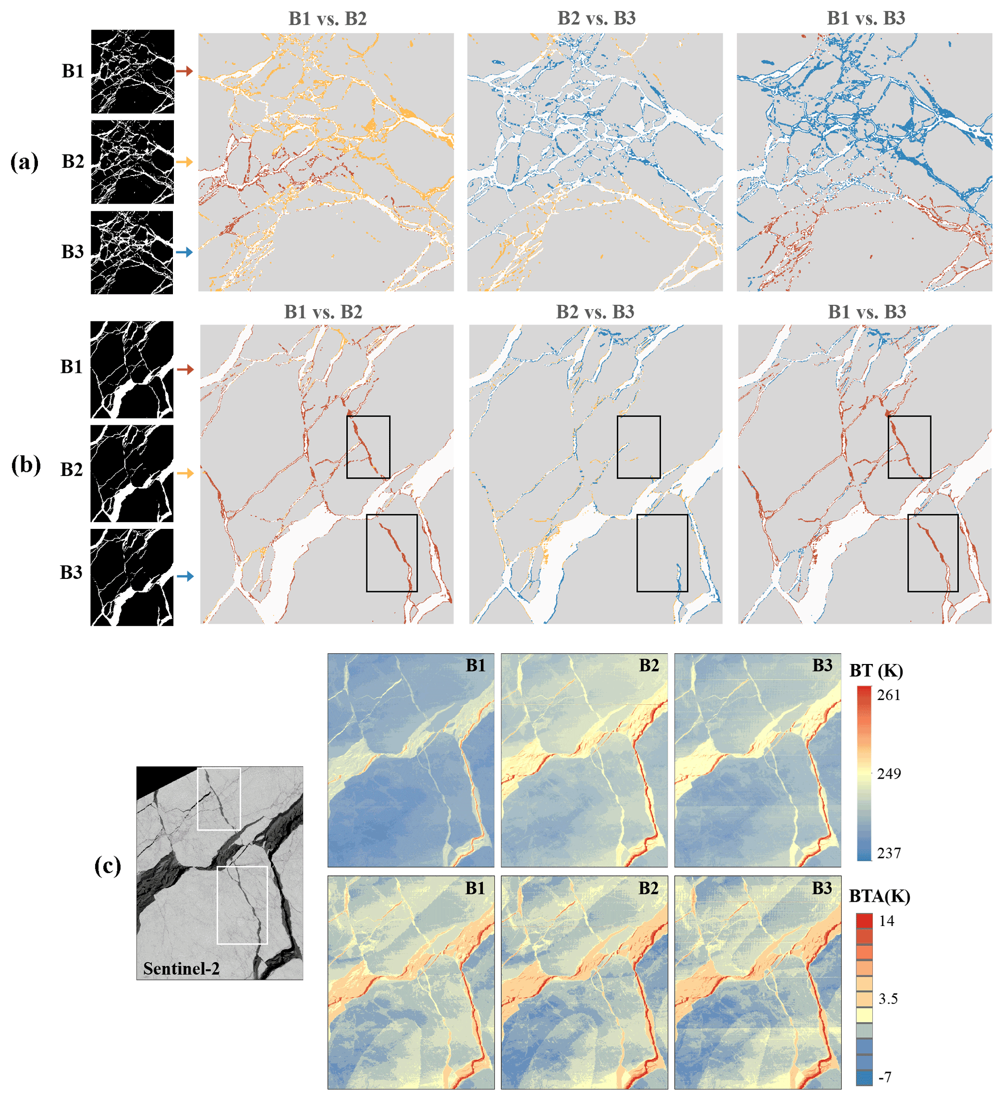
Figure 10 Cross-comparisons of lead detections among the three TIS bands. The first column in (a) and (b) shows detections by the three bands. The following three columns are pairwise comparisons, with dark red, orange, and dark blue representing the B1, B2, and B3 results, respectively. White pixels are consistency detections, and light gray indicates ice surface. Acquired from the same location as (b), the left panel in (c) shows the S2 image as a reference, with BT and BTA maps in two parallel rows. (a) TIS data acquired at 04:56 UTC on 28 April. ID: KX10_TIS_20220428_W147.26_N77.60_202200049406. Panels (b) and (c) are the TIS data acquired at 04:28 UTC on 3 April. ID: KX10_TIS_20220403_W132.14_N74.67_202200033227. (c) S2 data acquired at 21:00 UTC on 3 April.

To further investigate the discrepancies, we depicted the detections with different colors. As depicted in Fig. 10, dark red, orange, and dark blue colors represent the leads detected by the B1, B2, and B3 bands, respectively. The discrepancies primarily occur in the lead margins. Comparisons in the second (B1 vs. B2) and fourth columns (B1 vs. B3) in Fig. 10a indicate that the B1-derived leads are generally fewer than those from the B2 and B3 bands. The third column (B2 vs. B3) presents only a small number of spatial variations, probably due to local temperature gradients. Thus, it can be concluded that the TIS B2 and B3 bands yield comparable performances in detecting sea ice leads. These two infrared radiance bands, applied as the two split windows for temperature retrieval, are widely used in infrared sensors, e.g., the currently in-orbit Gaofen-5 (GF-5) Visual and Infrared Multispectral Sensor (VIMS), Landsat-8 TIRS, Landsat-9 TIRS-2, and MODIS on board Terra and Aqua.

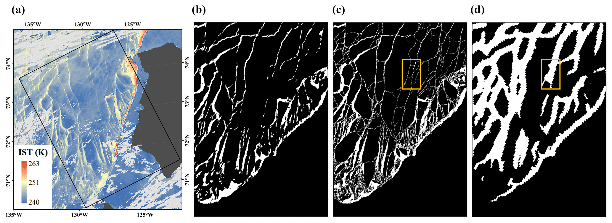
Figure 11 Comparisons of lead detections from MODIS and SDGSAT-1 TIS data in the Beaufort Sea on 3 April 2022. (a) MODIS IST product with off-white clouds, dark gray land, and overlaid black border denoting coverage for (b–d). (b) Lead detections at 1 km resolution from MODIS IST. (c) Lead detections at 30 m resolution from the combined result of TIS B1, B2, and B3 bands. IDs: KX10_TIS_20220403_W126.10_N71.30_202200033225, KX10_TIS_20220403_W128.84_N73.00_202200033226, and KX10_TIS_20220403_W132.14_N74.67_202200033227. (d) Lead detections at 1 km resolution from Hoffman et al. (2022b).

However, the scenario in Fig. 10b shows a different situation. There are more dark red pixels in the cross-comparisons. In particular, some dark red pixels (marked by the black squares) only present in the B1 band results, while the B2 and B3 bands almost lose all this information. Figure 10c shows the S2 visible images acquired in the same location, where the lead characteristics are evident (marked by white squares). Indeed, the BT and BTA maps found no apparent differences in the lead thermal characteristics. It is speculated that the missing data in the B2 and B3 bands may result from interference induced by strip noise, which is particularly pronounced in the two bands (a similar phenomenon is also present in the split-window channels of MODIS and Landsat 8 TIS). Regardless, this example suggests that using the TIS B1 band appears to achieve unexpected effects in the presence of interference in B2 and B3 data. In other words, the B1 band can be complementary to the two split-window bands. Thus, combining the results of the three bands is beneficial for resolving narrow leads with better accuracy.

4.3 Comparison of the TIS-derived sea ice leads with MODIS

We further compared the TIS-derived leads with the MODIS IST data at a moderate resolution. To achieve a fair comparison between the two sensors, we used analogous methods, as shown in a case study in the Beaufort Sea on 3 April 2022, depicted in Fig. 11a. The IST products were used to derive the BTA maps and applied a BTA threshold of 1.5 K for binary segmentation (Qu et al., 2021), which is also based on fixed thresholds (thus analogous to our proposed method). The MODIS-derived lead map is shown in Fig. 11b. Concurrently, as per the findings in Sect. 4.2, we combined our three lead maps, based on the three TIS bands, into one binary map, where the combined pixel is positive as long as any one of the three maps yields a positive pixel. The combined map contains the most leads, as shown in Fig. 11c. There is a significant difference between the high- and moderate-resolution results. The TIS resolves more lead details, e.g., the narrow leads connecting wide ones. Furthermore, some of the leads in Fig. 11c are even obtained in areas considered clouds by the MODIS cloud mask. Cloud-masked pixels were not compared for consistency purposes.

Table 7 Lead areas estimated from the MODIS IST data, the SDGSAT-1 TIS data, and Hoffman et al. (2022b).

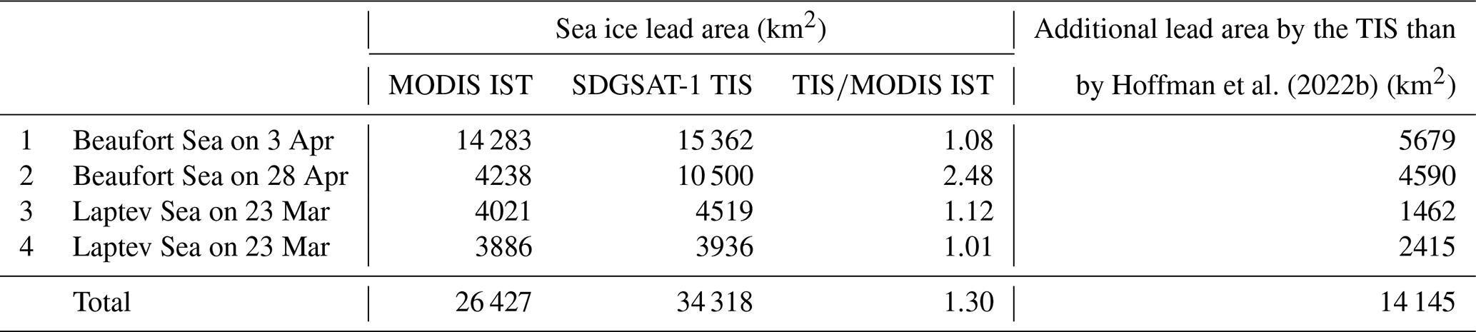
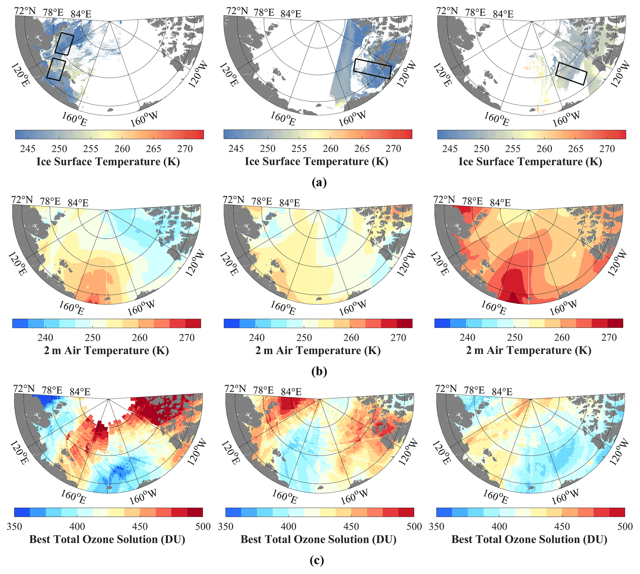
Figure 12 Temperature of ice surface and near-surface air and ozone solution for 23 March and 4 and 28 April 2022 (columns left to right). (a) MODIS IST, where black borders indicate the TIS acquisition range on the same day. (b) ERA5 2 m air temperature. (c) OMTO3 ozone solution.

Correspondingly, the lead area was calculated from both datasets in the same regions, as shown in the four regions in Fig. 1, and the comparison results are listed in Table 7. The area estimated from the TIS data is significantly larger than that estimated from MODIS IST, with the total area being 1.3 times larger than the latter. In particular, the difference in the lead area between the TIS and MODIS is the most significant for the case study in the Beaufort Sea on 28 April. The leads detected by the TIS are 10 500 km² in area (with the B1, B2, and B3 bands of 7752, 9346, and 8973 km², respectively). This could be attributed to the temperature variations on a short temporal scale. The IST increases to approximately 260 K in the Beaufort Sea on 28 April, far beyond the general IST range of 240 to 250 K for the study area (also see Fig. 12a). Consequently, the reduced thermal contrast of leads severely limits the ability of MODIS to detect leads. In contrast, the high-resolution imaging capability and high sensitivity of the SDGSAT-1 TIS can present more significant thermal contrasts of leads and ice.

Furthermore, Hoffman et al. (2022b) have published a lead dataset since 2002 for the season between November through April, which was detected by the U-net model (Hoffman et al., 2021) from MODIS 11 µm thermal imagery. This dataset has a spatial resolution of 1 km and reports the daily aggregated detection frequency. As shown in Fig. 11d, the lead widths and areas detected by this dataset are significantly larger, especially as small leads in close proximity are identified as one entire large lead (see the orange squares marked in Fig. 11c and d). Given that this dataset is not appropriate for the direct estimation of lead area, we used it as a binary mask and only calculated the area for the TIS-derived leads beyond this mask (i.e., the additional area). The statistics are presented in the last column of Table 7. The TIS-derived leads have an additional area of 14 145 km² compared to that derived by Hoffman et al. (2022b), which is generally in line with the comparison result between the TIS and MODIS IST. Thus, while the moderate-resolution sensor may over-represent the width and area of leads, the narrow leads overlooked under the kilometer-scale resolution are predominant. Since the width of leads strongly influences the turbulent exchange efficiency over them, the observation of leads at high spatial resolution is critical to achieve accurate lead width parameterization and estimate their thermal effects. These comparisons with the moderate-resolution sensor prove that the TIS is a competitive sensor for detecting sea ice leads in polar regions.

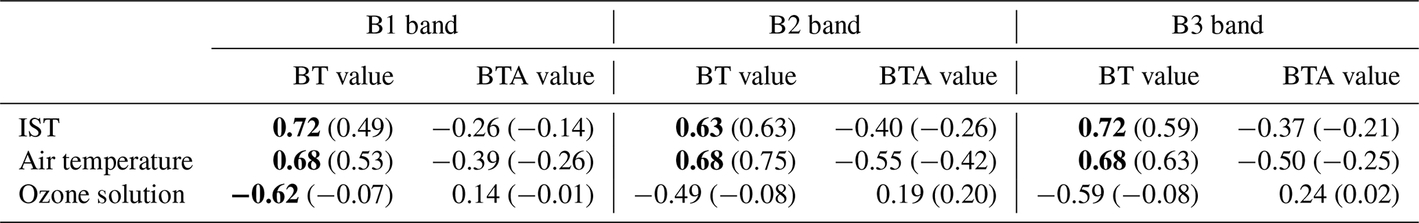
Table 8 Correlation between the thermal characteristics of the three SDGSAT-1 TIS infrared bands and the IST, 2 m air temperature, and ozone solution, with the slope of the regression fitting in brackets. The results with significant correlations are shown in bold.

5 Discussion

Based on the high-resolution thermal infrared data available from the TIS on board SDGSAT-1, we successfully detected sea ice leads in the Arctic at 30 m resolution, achieving good results in terms of the detection accuracy, adaptability, and ability to characterize narrow details. In this section, we focus on discussing the influence of different atmospheric conditions on uncertainties in TIS lead observation and analyzing the lead property revealed in the detection. This will provide insights into the factors affecting the accuracy of the TIS observation and the physical characteristics of the detected leads.

5.1 Atmospheric influence on sea ice lead detection by the three TIS infrared bands

First, as an important constraint on Arctic lead detection, it is necessary to consider the impact of cloud interference. Although cloudy conditions are prevalent in the Arctic (see the large white area in the MODIS daily IST product shown in Fig. 12a), due to the unavailable cloud products synchronized with the SDGSAT-1 TIS, this study only demonstrates the lead detection under clear-sky conditions. However, we agree with the view of Hoffman et al. (2019) that using cloud mask products in lead detection would produce omissions as a result of incomplete cloud information. They reclassed the MODIS cloud mask products to eliminate omission errors and assumed that a lead pixel would have a BT less than 271 K (otherwise, it would be open water or warm cloud). We manually collected cloudless data and used the BT filter, which rejected pixels with BT values lower than approximately 245 K. Therefore, clouds are likely to have a relatively small impact on the results of this study, but the impact of warm clouds still remains. In the future, with the availability of the SDGSAT-1 cloud product, we can further investigate lead detection for cloudy conditions.

Apart from cloud interference, other atmospheric components also affect lead detection. The TIS B2 and B3 bands, the two atmospheric windows, are nearly transparent to the atmosphere, and therefore, to some extent, they can obtain surface radiance independent of the atmosphere. In contrast, the B1 band, as an absorption channel for ozone (Wan and Li, 1997), has attenuation in the atmosphere. As a result, the B1 band data present different temperature gradients from the other two bands, which are particularly pronounced at high latitudes (Prabhakara and Dalu, 1976). In addition, short-term temperature variations also affect the temperature contrast for the three thermal infrared bands and thus the detection of leads. Since the at-sensor BT data used in this study were not corrected for atmospheric radiation, this temperature variation results from a combination of sea ice radiation and atmospheric radiation. As displayed in Fig. 12, the temperature of the sea ice surface and 2 m air and the ozone solution present significant temporal and regional variations. Both the air and ice temperatures gradually increase and show similar spatial patterns. The ozone solution is high in the Laptev Sea and the Beaufort Sea, and its distribution changes rapidly on a monthly scale. We analyzed the sensitivity of lead temperature characteristics to these factors. First, based on the detected leads, we extracted the BT and BTA data only for those lead pixels and allocated them to geographic grids at 30 km resolution (1/10th of the TIS swath width to allow comparison with coarse-resolution datasets). Then, a regression analysis was conducted to find the relation between the thermal characteristics and IST, air temperature, or ozone solution, as listed in Table 8.

In general, the BT data from the three TIS bands show significant positive correlations with the IST and air temperature. Although the upward slope of the BT data with respect to ice and air temperatures for the B1 band is smaller than that for B2 and B3 bands, the high correlation (0.72 with the IST and 0.68 with the air temperature) demonstrates its effectiveness as a thermal infrared band for lead detection. On the other hand, changes in IST have only a small negative correlation with the BTA values of leads, while changes in air temperature are more likely to diminish the thermal contrast of leads, which have less effect on the B1 band and more effect on the B2 band. These results imply that atmospheric correction and ice temperature retrieval of TIS thermal data could be effective approaches to improve the robustness of lead detection. Among the three thermal infrared bands of the TIS, the B1 band may not be as sensitive to temperature variations as the B2 and B3 bands.

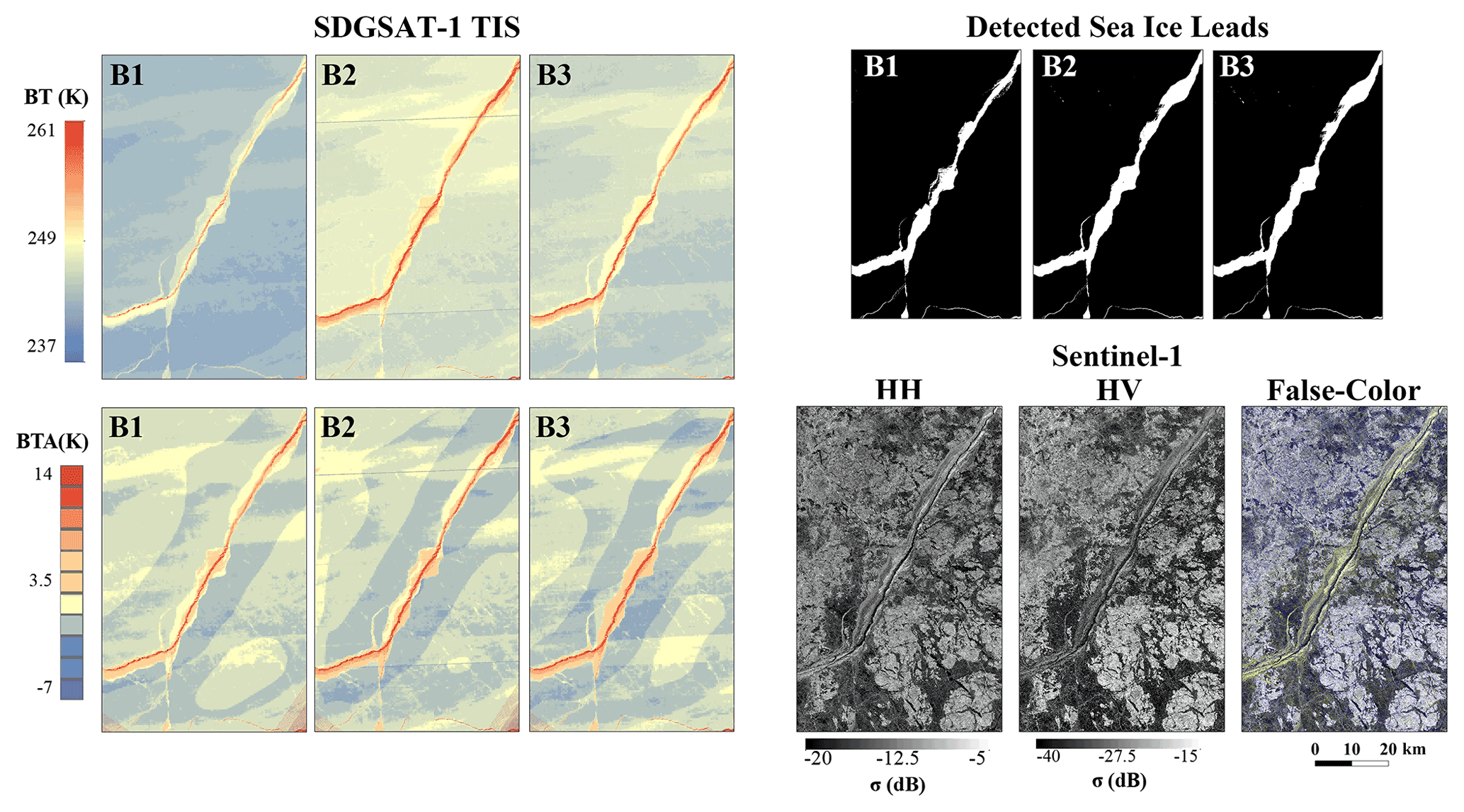
Figure 13 Comprehensive analysis for lead property in the Beaufort Sea based on SDGSAT-1 TIS data acquired at 04:28 UTC on 3 April and the matched S1A data at 15:53 UTC on the same day. Two parallel rows of panels on the left show the BT and BTA maps for the three bands of SDGSAT-1 TIS. The first row on the right panel shows the leads detected in this study. The panel at the bottom right displays the matched S1A HH, HV, and false-color composite images. SDGSAT-1 TIS data ID: KX10_TIS_20220403_W132.14_N74.67_202200033227.

As we expected, only the BT data from the B1 band exhibit a negative correlation with ozone, with a correlation of −0.62. This result is not surprising since only the B1 band radiance is heavily absorbed by ozone, which also explains why the B1 band yields the lowest BT values for the presented cases in this study. With respect to the BTA values of leads, none of them show significant correlations with the ozone solution. This finding implies that although ozone affects the B1 band temperature measurement, it barely weakens the thermal contrast required for lead detection.

5.2 Sea ice lead property resolved by the TIS

Due to thermal infrared imaging having long been limited to the moderate resolution of kilometers, it is difficult to confirm either the widths of narrow leads or the variations within them. The detection at the 30 m resolution allows for thermal variations to be observed within leads, as demonstrated in an interesting case shown in the two-row panels on the left of Fig. 13, which was acquired on 3 April over the Beaufort Sea. The TIS data present a noticeable transition zone (with a BTA value less than 2 K), which is likely seawater intrusion into the sea ice while the lead in the center (with a BTA value greater than 3 K) was just opening. As the method used in this study aims to extract all potential leads, the entire transition zone was marked as a lead. This is reasonable, as a previous study (Qu et al., 2021) used a BTA threshold of 1.2 K for potential leads, 1.5 K for general leads, and 2 K for open water discrimination. Given that the binary segmentation in this study applies a 1.8 K threshold, it again indicates that the thermal information obtained by SDGSAT-1 TIS presents a more significant thermal contrast.

Broadly speaking, fracture zones covered by thin ice and intruded by seawater are also considered leads. For other supporting evidence, we incorporated the S1A SAR images acquired on the same day. Murashkin et al. (2018) developed an automated S1 lead detection algorithm. It should be noted, however, that this algorithm may have limited applicability for complex scenarios that involve a potential transition zone between thin ice and seawater. In contrast, the use of quantitative backscatter data obtained from dual-polarized S1 images has been found to offer improved distinguishability. The HH and HV SAR data, as well as the false-color composite images, are presented in the panel at the bottom right of Fig. 13. The overall backscatter values for the HH and HV data are low. However, in the transition zone of the lead, the backscatter values of the HH and HV data differ considerably, while both the backscatter values are very low at the center opening. Accordingly, the transition zone is yellowish in the false-color composite image, whereas the opening lead is darker. Hence, the leads detected in this study based on thermal contrast are consistent with the properties resolved by the polarization differences in SAR. Regarding the application of SAR data to lead detection, its applicability to local sea ice conditions remains to be further explored.

In addition, contours of multiyear ice with high backscatter values observed in SAR images are similar to some negative BTA features. Such surface information is particularly sensitive to the B2 band, suggesting surface temperature variations for different thicknesses of sea ice. Similar surface temperature variations are also found in the 1 m resolution IST data obtained from helicopter-borne thermal infrared imaging (Thielke et al., 2022). Thanks to the high-resolution characterization of the SDGSAT-1 TIS and the accurate radiometric measurement, it is possible to reveal the sea ice properties both inside the leads and on the ice surface. However, for sea ice with a high-temperature characteristic, possibly due to thicker or local temperature gradients, its BTA can be similar to that of a lead and can be difficult to distinguish (Key et al., 1993), which is why we preferred a BT filter after the lead segmentation in this study.

The special case shown in Fig. 10b and c arouses our interest in understanding why the B2 and B3 bands missed some leads. As described in Sect. 4.2, the strip noise also affects lead detection. The strip noise is the most severe in the B3 band and secondly in the B2 band, while it is absent in the B1 band. This discrepancy arises due to the fact that when the TIS overpasses a homogeneous surface, which covers sea ice with a low radiance signal in this case, each detector generates a different noise bias (Corsini et al., 2000). This phenomenon is even more pronounced for detectors with higher signal-to-noise ratios. Likewise, to overcome the strip noise, it is necessary to apply the BT filter and use an appropriate threshold. In this case, the thresholds determined through iterative selection were 243.93, 248.02, and 247.14 K for B1, B2, and B3, respectively. Consequently, the high thresholds of B2 and B3 caused some lead details to be omitted during the detection process. From this perspective, residual noise in high-resolution thermal infrared images may have an impact on the lead detection based on the TIS B2 and B3 bands, whereas the B1 band is less susceptible due to its relatively low sensitivity. It is noted that the forthcoming level-4b TIS data can suppress some of the stripe noise. On the other hand, as the TIS data available within the scope of this study are relatively limited, the individual case studies presented may be weak in terms of generalizability. In the future, with the support of a large amount of data, we aim to develop a method that can overcome various interferences for application to SDGSAT-1 TIS data to more accurately detect sea ice leads.

6 Summary and conclusion

Over the past decades, the Arctic has experienced increasing temperatures and a rapid retreat of sea ice, with profound implications for both the Arctic and the extra-polar climate and ecosystems. Sea ice leads play a critical role in regulating the heat exchange between the ocean and the overlying atmosphere. However, previous lead observations based on thermal infrared remote sensing have long been limited to moderate resolutions on a kilometer scale, making it challenging to resolve lead details and resulting in inadequate estimates for lead parameters. There is an urgent need to develop a fine-scale dataset of sea ice leads.

The recently launched SDGSAT-1 provides an emerging opportunity to detect leads at high spatial resolutions up to 30 m by its onboard TIS payload. This study demonstrates the feasibility of using the three TIS infrared bands for detecting leads in the Arctic Ocean. We proposed a method that combines binary segmentation with the BT filter to detect leads by the three TIS bands. The detection results show great details on narrow leads of tens of meters in width, as well as high accuracy. For example, in the Beaufort Sea case in April 2022, the overall accuracies are 96.2 %, 96.3 %, and 96.3 % for the B1, B2, and B3 bands, respectively, compared with the S2 visible images at 10 m resolution. Since more narrow leads are detected by the TIS, the TIS-derived lead areas are 1.3 times more than the results based on the MODIS IST data at a 1 km resolution in the 11 collected cases. Our finding indicates that more leads exist in the Arctic Ocean than we have ever observed. These narrow leads beyond our expectations would allow for more heat exchange (Marcq and Weiss, 2012). Therefore, the TIS sensor is expected to improve the lead representation, which is crucial for climate models.

The cross-comparisons among the three TIS infrared bands suggest that the B2 and B3 bands have similar performances in detecting leads, whereas the B2 band yields the best performance among the three bands. Although the B1 band is less commonly used in thermal infrared measurements, the leads detected by the B1 band can be complementary to the other two on some occasions. We therefore recommend using the combined results of the leads detected from the three TIS bands and also intend to further explore the adaptability of combining different thermal infrared bands and their potential for improved lead detection in the future.

The analysis of the correlation between the detected leads and temperature suggests that the B1 band (both its BT and BTA data) is less sensitive to variations in surface and near-surface temperature. Although ozone in the atmosphere absorbs B1 band radiance, ozone has little impact on lead detection by the B1 band. The different sensitivity of the B1 band to surface information and atmospheric conditions from the other two bands produces an unexpected performance in sea ice lead detection, allowing it to complement the other two bands (and being an important underpinning for IST retrieval). Regarding the variations inside the leads, an analysis incorporating the S1A data agrees with the lead properties revealed by our results, but the threshold currently used does classify the transition zone as a lead. Thanks to the sufficiently high resolution of the SDGSAT-1 TIS, it is expected to provide crucial data for the analysis of lead formation and refreezing based on sequential thermal infrared data, an aspect that deserves future attention.

This study investigates the detection of sea ice leads by spaceborne thermal infrared remote sensing at a high spatial resolution of tens of meters. The results demonstrate that the TIS on board SDGSAT-1 has excellent potential for detecting sea ice leads (as well as possible IST retrieval) in polar regions. Nevertheless, limited by the imaging time and cloudy conditions over the Arctic region, only individual case studies based on TIS data were carried out, which may result in weak generalizability. Along with the acquisition of additional TIS data over the course of a year, as well as the development of a near-real-time cloud product, we plan to develop a long-term lead dataset based on SDGSAT-1 TIS at 30 m resolution to support research on the dynamics of sea ice and expect to investigate the lead detection capabilities of this dataset across different seasons. Combining this dataset with diverse datasets of sea ice, we aim to provide insights into the contribution of sea ice leads to Arctic sea ice dynamics, an effort to combat climate change and its impacts as a key towards SDG 13: climate action.